Article

Subsampling and Aggregation: A Solution to the Scalability Problem in Distance-Based Prediction for Mixed-Type Data

1
Departamento de Matemáticas, Universidad Autónoma de Madrid, 28049 Madrid, Spain
2
Statistics Department, Universidad Carlos III de Madrid, 28903 Getafe, Spain
*
Author to whom correspondence should be addressed.
These authors contributed equally to this work.
Mathematics 2021, 9(18), 2247; https://doi.org/10.3390/math9182247
Submission received: 8 July 2021 / Revised: 2 September 2021 / Accepted: 8 September 2021 / Published: 13 September 2021
(This article belongs to the Special Issue Multivariate Statistics: Theory and Its Applications)

Abstract

:
The distance-based linear model (DB-LM) extends the classical linear regression to the framework of mixed-type predictors or when the only available information is a distance matrix between regressors (as it sometimes happens with big data). The main drawback of these DB methods is their computational cost, particularly due to the eigendecomposition of the Gram matrix. In this context, ensemble regression techniques provide a useful alternative to fitting the model to the whole sample. This work analyzes the performance of three subsampling and aggregation techniques in DB regression on two specific large, real datasets. We also analyze, via simulations, the performance of bagging and DB logistic regression in the classification problem with mixed-type features and large sample sizes.

1. Introduction

The sources collecting all types of information from citizens are ubiquitous and increasing in number and voracity. Thus, the nature of data is, more than ever, of mixed type, that is, at least each individual gives rise to quantitative and qualitative variables, but also textual and functional data or even manifolds. Many classical multivariate analysis techniques have been initially proposed to deal with quantitative data. However, statistical problems involving multivariate mixed data can also be solved via an adequate inter-object metric.
Computing the distances or similarities between pairs or groups of sample individuals is, thus, a way of summarizing sample information that allows using any kind of random object or mixtures of different kinds. In this work, we focus on data mixing of both qualitative and quantitative variables, but the procedures can potentially be used with very general data objects as long as pairwise distances can be computed between them (see, e.g., the functional framework analyzed in Boj et al., 2010 [1] or the manifold distances considered in Wang et al., 2012 [2], Shao et al., 2014 [3] and in Tsitsulin et al., 2020 [4]). Some statistical techniques, such as certain clustering procedures or multidimensional scaling (MDS), use only the matrix of pairwise distances as an input to perform the procedure. The distance-based linear model (DB-LM) first uses the metric version of MDS to extract a Euclidean configuration of the distance matrix and then performs linear regression of the response variable on the configuration. The DB-LM technique, introduced by Cuadras (1989) [5], was developed by Cuadras and Arenas (1990) [6] and Cuadras et al. (1996) [7] and extended to the framework of functional data by Boj et al. (2010) [1] and to the case of generalized linear models by Boj et al. (2016) [8].
Obviously, when the sample size n is very large, the dimension n × n of the matrix of pairwise distances between sample individuals can be prohibitively large to carry out DB regression. Ensemble methods (see [9,10] and references therein) offer flexible ways of dealing with large sets of observations. In particular, subsampling and aggregation techniques such as bagging (Breiman 1996a [11]) or stacking (Breiman 1996b [12]) have proved useful when dealing with large or high-dimensional data sets in the context of regression and classification (Bühlmann 2003 [13]). Further, big data sets frequently have an inhomogeneous structure due to, e.g., the presence of outliers or mixed populations. Bühlmann and Meinshausen (2015) [14] proposed maximin aggregation (magging) to adapt the subsampling and aggregation techniques in linear regression to large samples of heterogeneous observations.
The aim of this work is to assess the impact of subsampling and aggregation strategies on the performance of distance-based linear and logistic regression models. Specifically, we apply bagging, stacking, and magging to the framework of DB linear regression, with the aim of circumventing the problem posed by the computational unfeasibility of decomposing the Gram matrix as well as the storage of the distance matrix when n is so large. We discuss the results for a varying number of sizes and samples in terms of mean squared prediction errors, median absolute prediction errors, and computational complexity. In the context of mixed data, it is not clear which model could be appropriate to generate simulated samples, so in this work the performance of the ensemble methods in the regression context is tested on two large, real datasets. One of the conclusions derived from this analysis is that bagging is very competitive compared to stacking and magging, both in terms of computing time and complexity and of the mean squared prediction error. This has led us to investigate the performance of bagging in the classification problem when using distance-based logistic regression (see [8]). Computationally speaking, this problem is more complex, and model fitting takes longer time than in the regression case (since the least squares fitting procedure is replaced by an iterative weighted least squares algorithm; see McCullagh and Nelder [15], Section 2.5), so selecting bagging as the ensemble technique is advantageous. We have carried out a simulation study to compare the performance of bagging applied to DB logistic regression and of the classical logistic regression model fitted to the whole sample. In Figure 1, we provide a flowchart to illustrate the procedure for using DB prediction models in large sample sets.
The paper proceeds as follows. In Section 2, we recall the framework for distance-based regression, as well as notation and the basic expressions for DB linear prediction of a response variable, and we comment on its extension to the generalized linear setting; we introduce Gower’s distance as the classical metric to deal with mixed-type data; we summarize the essentials in the procedures of bagging, stacking, and magging, which clarifies their potential, straightforward use in DB regression. In Section 2 we describe two real bases of mixed-type data on which we evaluate the performance of the ensemble techniques. Section 3 summarizes the results of applying the ensemble techniques reviewed in Section 2.3 to DB linear and logistic regression. A final discussion is given in Section 4. All the DB regressions were carried out using the R package dbstats (Boj et al., 2017 [16]).

2. Materials and Methods

2.1. Distance-Based Linear and Logistic Regression

In this section, we establish the basic ideas and notation for the procedure of distance-based linear regression. As pointed out in the end of the section, the extension of these ideas to generalized linear models is straightforward, although their computational implementation is not as simple. For the sake of clarity, the formulas and intuition behind the DB methodology are kept to the minimum possible (see [1] for more mathematical details). Distance-based (DB) regression is a prediction procedure that can be applied to qualitative or mixed regressors. It is performed in two steps: from a matrix of pairwise distances between sample individuals, via MDS we obtain latent variables, which are then used as predictors in least squares linear regression. The advantage of DB regression is that it does not depend on the choice of the latent regressors, since the predicted response depends solely on the distance matrix (see Theorem 1 in [1]). When all the predictors are quantitative and the metric between the sampled individuals is the Euclidean one, then the DB linear regression is equivalent to the classical least-squares linear regression (see [6]).
Assume that we have taken a sample of n individuals from the population of interest. For each of them we observe the value of a response variable Y and a “vector” Z of predictive variables, some or all of which can be qualitative. Let y i denote the value of Y in the i-th individual and y = ( y 1 , , y n ) . Let ω i ( 0 , 1 ) be the positive weight of the i-th individual in the sample, ω = ( ω 1 , , ω n ) , the weight vector, satisfying i = 1 n ω i = 1 , and consider a diagonal matrix D ω = diag ( ω ) , whose diagonal is equal to vector ω .
The values of Z for the n individuals are z 1 , , z n . We assume that a distance or dissimilarity δ can be defined between any two possible values of Z . Denote by Δ the n × n symmetric matrix whose entries are the squared distances δ 2 ( z i , z j ) .
We define the n × n inner products or Gram matrix as
G ω = 1 2 J ω Δ J ω ,
where J ω : = I 1 ω is the ω -centering matrix. Here I is the n × n identity matrix and 1 is an n × 1 vector of 1s. If an n × k matrix X ω satisfies G ω = X ω X ω , then X ω is a k-dimensional Euclidean configuration of Δ . The inner-products matrix G ω admits such a decomposition in terms of an Euclidean configuration if and only if G ω is a positive semidefinite matrix. Intuitively, the rows of the Euclidean configuration X ω are n observations of a latent regressor in R k such that the pairwise Euclidean distance between rows i and j match δ ( z i , z j ) , for  i , j = 1 , , n . The key idea in DB regression is to substitute the original “matrix” of observed mixed-type predictors Z by X ω in the regression problem. DB-LM implicitly performs the weighted least-squares (WLS) linear regression of the response vector y on the row space of the Euclidean configuration X ω .
The results of the DB-LM procedure do not depend on the choice of a specific Euclidean configuration (see [1]). Indeed, to clarify this point, in the following lines we detail the expression of the predicted response y ^ in DB-LM. To this end, we define first the DB-LM hat matrix as
H ω = G ω D ω 1 / 2 F ω + D ω 1 / 2 ,
where F ω + is the Moore-Penrose pseudo-inverse of
F ω = D ω 1 / 2 G ω D ω 1 / 2 .
Consequently, the sample values of the response Y predicted using DB-LM are (see [8])
y ^ = y ¯ ω 1 + H ω ( y y ¯ ω 1 ) ,
where y ¯ ω = ω y the weighted sample mean of y . For a new individual with predictor values given by z n + 1 , the fitted response given by DB-LM (derived from the interpolation formula in Gower 1968 [17]) is
y ^ n + 1 = y ¯ ω + 1 2 ( g ω δ n + 1 ) D ω 1 / 2 F ω + D ω 1 / 2 ( y y ¯ ω 1 ) ,
where g ω is the n × 1 vector containing the diagonal entries of G ω and δ n + 1 is the column vector of squared distances from z n + 1 to z 1 , , z n . Observe that neither (3) nor (4) depends on choosing any particular configuration X ω . In Figure 2, we illustrate the the process to predict a new case with DB-LM through a block diagram.
The DB-LM was extended to the generalized linear model (GLM) setting by Boj et al. (2016) [8]. The key is to substitute the linear regressions, carried out in the iterative weighted least squares (IWLS) algorithm for GLM fitting, by the corresponding DB-LMs. In particular, DB logistic regression (also implemented in the dbstats library) can be used to solve classification problems with mixed-type data (see also [18] for a mixed-features classification procedure based on a general model for the joint distribution of the features). In some preliminary simulations, we compared the performance of the logit and probit links and there were no significant differences in the attained errors.

2.2. The Choice of the Distance

The choice of the metric between observations of a general random object is a key element in this context. In general, two very different individuals, statistically speaking, may appear to be very close in an erroneously chosen metric. Even if the Euclidean distance is computationally simple to obtain, we remark that the practice of encoding categorical variables with some arbitrarily chosen, real numbers and applying multivariate techniques, suitable only for quantitative data, to these numerically-encoded data is not reliable.
A more adequate distance measure for mixed data was proposed by Gower (1971) [19]. Given two observations z i and z j of a mixed-type random vector Z , Gower’s similarity coefficient is defined as
s i j = h = 1 p 1 1 | z i h z j h | / R h + a + α p 1 + ( p 2 d ) + p 3 , 0 s i j 1 ,
where p 1 is the number of quantitative variables in Z , a and d are, respectively, the number of coincidences ( 1 , 1 ) and ( 0 , 0 ) for the p 2 binary variables, α is the number of coincidences in the p 3 multi-state (not binary) qualitative variables, and R h is the range of the h-th quantitative variable. Gower’s distance is defined as δ 2 ( z i , z j ) = 1 s i j . There are other possible, more robust, metrics that can be used with mixed data (see, e.g., [20]), but, for simplicity, we use Gower’s distance, as it is implemented in the R cluster package and supported in the dblm and dbglm functions of the dbstats package that we employed in the analysis of the real data sets and in the simulations.

2.3. Some Ensemble Regression Techniques

Currently, it is common to encounter data sets with such a large sample size n that the decomposition of the resulting Gram matrix (1) cannot be performed, or even that the computation and storage of the squared-distances matrix are unmanageable. The problem regarding the Gram matrix is due to the unfeasibility of performing the eigendecomposition of the matrix F ω in (2) for very large data sets. In the context of MDS, this issue has been addressed, for instance, by Paradis (2018) [21] and Grané and Sow-Barry (2021) [22]. To address the computational problems posed by this situation and at the same time maintain statistical efficiency, a simple approach is to use ensemble techniques (see [14,23]). Specifically, in this work we use subsampling (which, for each input of the vector of predictors, generates several predictions for the corresponding response) and aggregation (which combines the predictions into a single output).
Let G 1 , , G G , with  G g { 1 , , n } , denote subsample index sets. The subsamples may be overlapping; that is, G g G g for some g g . For each subsample G g , g = 1 , , G , we predict the value of the response in the new individual, y ^ n + 1 ; g . These ensemble predictions y ^ n + 1 ; 1 , , y ^ n + 1 ; G can be aggregated to a single predicted response y ^ n + 1 ; a g g r in different ways (see [14]).
For the procedures of stacking and magging described in Section 2.3.1, the final response prediction requires computing a collection of certain weights. In the optimization steps to compute the weights, it is necessary to predict the response for each subsampled individual. Thus, it is important to take care of the following technical details. We can use all the observations in subsample G g , for any fixed g = 1 , , G , to compute the predicted response y ^ i ; g for the i-th sampled individual, i = 1 , , n . However, if G g contains that particular i, then we would be using “inside information” to predict y i . To prevent this, for each g = 1 , , G we denote y ^ ( g ) = ( y ^ g ( 1 ) , , y ^ g ( n ) ) the vector of predictions for the sample individuals based on the g-th subsample from which the i-th individual in the original sample has been deleted (so y ^ g ( i ) = y ^ i ; g if i G g ).

2.3.1. Aggregation Procedures for Regression

In this subsection we review three aggregation procedures used in the context of standard linear regression, namely, bagging, stacking, and magging. Conceptually, they have a straightforward extension in the case of DB-LM, but as far as we know there are yet no empirical studies evaluating their practical performance in this setting. In this work, we test the following three aggregation procedures over two real data sets.

Mean Aggregation and Bagging

In the bagging technique, proposed by Breiman (1996a) [11], the prediction of the response is the average (with equal weights) of the ensemble predicted values
y ^ n + 1 B : = g = 1 G v g y ^ n + 1 ; g ,
where v g = 1 / G , for all g = 1 , , G .

Stacking

Stacking was introduced by Breiman (1996b) [12] and Wolpert (1992) [24]. In this case, the prediction of the response is a weighted average of the subsample predictions
y ^ n + 1 S : = g = 1 G v g y ^ n + 1 ; g ,
where
v = ( v 1 , , v G ) =   arg min v V y g = 1 G v g y ^ ( g ) 2
The space V of possible weight vectors v can be one of the following
V c = { v : min g v g 0 , g = 1 G v g = 1 } ( convex constraint ) V r = { v : v 2 s } for some s > 0 ( Ridge constraint ) .

Magging

To deal with possible data inhomogeneity, Bühlmann and Meinshausen (2015) [14] proposed the prediction of the response as a weighted average of the ensemble predictions
y ^ n + 1 M : = g = 1 G v g y ^ n + 1 ; g ,
with weights such that
v = arg min v V c g = 1 G v g y ^ ( g ) 2 .
We have used the R package quadprog to compute these weights, as suggested by these authors.

2.3.2. Bagging for Classification

It is natural to try to evaluate the same three aggregation techniques reviewed in Section 2.3.1 in the classification context. However, at the time of writing this manuscript, magging had not yet been extended to the discrimination framework. Stacking is indeed a popular meta-classifier procedure among the machine learning community. Stacking for classification consists in two steps (as in stacked regression). The first step (base-level classification) is to use the G subsamples from the training sample to generate G predictions of the class to which each individual in the training sample belongs. These predictions can be the class or the probability of belonging to each class. The second step (meta-level classification) is to use the learned classifiers, obtained in the base level, to generate final predictions of the classes of the training sample individuals. After training these two classifiers (in the base and meta level), one can classify a new observation (see Džeroski and Ženko 2004 [25] for a review of stacking classifiers). In our case, the first step could be performed via DB-GLM, but the use of DB-GLM in the second step is not computationally feasible (if the training sample is too large it would require a further, nested ensemble procedure). The practical implementation of the subsampling and aggregation techniques carried out in Section 3.1 allows us to conclude that, for adequate choices of the number G of subsamples and the subsample size m, bagging attains a mean squared error that is, at least, among the lowest. Bagging is also the fastest way to compute of the three aggregation techniques revised in Section 2.3.1. Since DB-GLM is more involved, computationally speaking, and takes longer to be fitted to data than DB-LM, we have chosen bagging as the only aggregation technique to be applied to DB logistic regression.
In the classification problem with two populations, the values of the response Y take only two values (0 or 1), depending on the population where the individual was drawn from. Thus, the response (classification) y ^ i ; g , predicted for the i-th individual on the basis of the g-th subsample, is also a binary, 0–1, value. In this case, the bagging aggregation procedure consists in taking the vote of the majority:
y ^ n + 1 B = arg max k = 0 , 1 g = 1 G 𝟙 { y ^ i ; g = k } .

2.4. Databases under Consideration

In this work we apply the ensemble techniques reviewed in Section 2.3 to a pair of real data sets. Here we describe in detail these data collections as well as the choice of the parameters in the algorithms.
Let us first give some general comments applying to both sets. Although, in practice, the number G of subsamples can be chosen via cross-validation (see [26]), in this work we have decided to compare the performance of the ensemble procedure for different choices of G. Once G is fixed, a simple way to choose the size m of each subsample G g , for all g = 1 , , G , is to take m = [ n / G ] . For each g, the subsample G g is formed by sampling m individuals from { 1 , , n } without replacement.
The analysis performed on the data sets is a Monte Carlo experiment, with a total number of runs equal to 500. In each Monte Carlo run, to compare the different procedures under consideration, first we randomly separate the original sample into a training sample of size n approximately equal to 90% of the original sample size and a test sample with the remaining observations. Thus, each method’s performance was evaluated by repeated random sub-sampling validation or Monte Carlo cross-validation. In particular, to quantify the performance of each method, we compute (i) the distribution, average and standard deviation of mean squared error (MSE) in the prediction of Y for the individuals in the test sample, computed from 500 runs within each scenario; (ii) the distribution of the median absolute prediction errors (MAE) also computed from 500 runs within each scenario; (iii) the complexity of the method (time and memory).

2.4.1. Bike Sharing Demand

This dataset is provided by the Capital Bikeshare program and it is available at their website (www.capitalbikeshare.com/system-data, accessed on 3 June 2019). Capital Bikeshare operates in the District of Columbia, Arlington County, VA, and the City of Alexandria, VA. The program records several details, such as travel duration, departure and arrival locations, and time elapsed between departure and arrival, for each rental in the bike sharing system.
We have chosen to analyze the data on a daily basis (hourly information was also available) for the period between 1 January 2013 and 31 December 2018. The scarce days for which data were not available were deleted from the sample. The variables appearing in the Capital Bikeshare files for each day are listed in the first part of Table 1. To the data provided by Capital Bikeshare (year, month, day, and count of users) we added, for each day, variables describing weather conditions that could affect the decision of picking up or not a bike (second part of Table 1). This information at Ronald Reagan Washington National Airport (DCA) was gathered from the website of the National Oceanic and Atmospheric Administration (NOAA). The reason for choosing the specific DCA location was to ensure data availability for all days of interest and also because it is centered in the area covered by the bike stations, and thus it is a good representative. The NOAA variables in the second part of Table 1 are treated as quantitative ones. The variables in the first part of Table 1 are treated as qualitative ones (declared as factors in R), except for the total count of daily users. The response variable Y is the daily count of users (casual and registered) scaled by the mean daily number of users (in the year corresponding to the day). The total number of days in the data set is 2903.

2.4.2. King County House Sales

This dataset comes from Kaggle (www.kaggle.com, accessed on 12 July 2019) and contains house prices from King County (Washington State, USA), sold between May 2014 and May 2015. The dataset consisted of 20 variables (see Table 2) and 21,597 individuals (houses). We removed the three (outlying) lots with an area of more than 500,000 sqft. The response variable we consider is the logarithm of the house sale price.

3. Results

3.1. Aggregation and DB-LM on Two Real Data Sets

3.1.1. Bike Sharing Demand

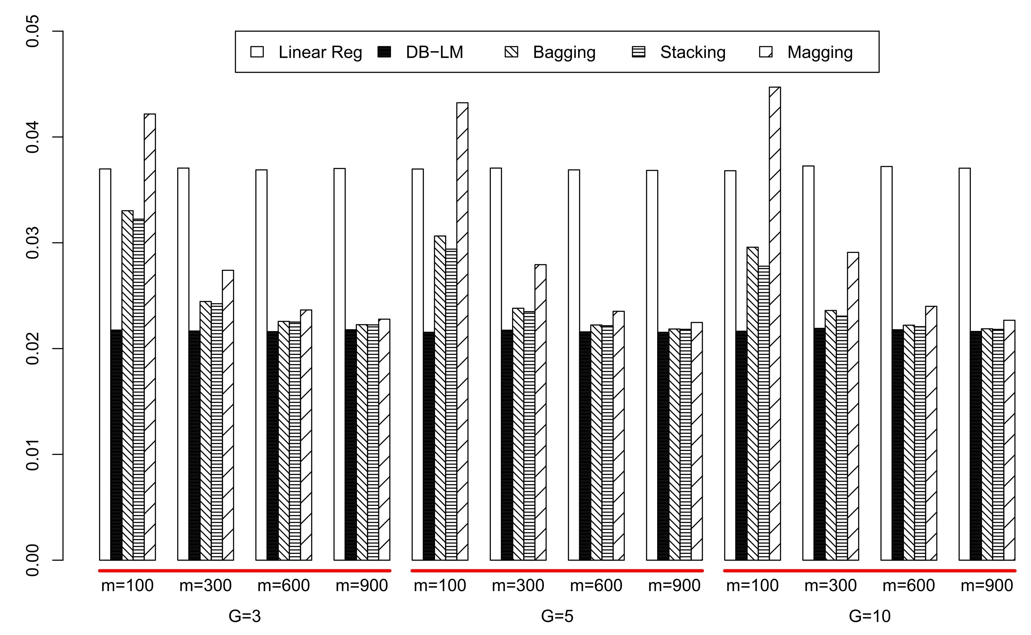
Let us fix the values of the technical parameters in the subsampling, aggregation, and overall analysis. In each of the Monte Carlo runs, the sample was randomly divided into a test sample (of 290 individuals) and a training one (of size n = 2613 ). We have tried three different numbers G of subsamples: 3, 5 and 10 and three different values for the subsample size, m = 100 , 300, 600 and 900. For this specific dataset, of relatively low size, we have been able to compute the predicted responses in the test sample using DB-LM on all the training sample. Thus, we are able to compute the mean squared error attained using all the training information simultaneously in the classical linear regression (only with the quantitative predictors) and the DB-LM. These results are compared with the MSE obtained with the ensemble procedures.
In Table 3, we display the average and standard deviation of mean squared prediction errors (MSE), computed from 500 iterations, for the subsampling and aggregation methods. With linear regression, DB-LM and random forests (R-package ranger with 100 trees, mtry = 7, depth = 20) the MSE is, respectively, 0.03700, 0.02168, and 0.01746. In Figure 3, we show the mean squared errors for all the regression methods. For this data set, it is clear that the number G of subsamples does not have a great influence on the MSE: this is good news since increasing G increases also noticeably computation time and memory requirements. In Table 4, we see the subsample size m and the overall number G m of observations used as input in the ensemble predictions. From Table 3 and Table 4 and Figure 3, we can see that, for  G = 3 and m = 600 , even if G m = 69 % is considerably below 100%, the three aggregation procedures are very near the MSE of DB-LM using the whole sample. Bagging and stacking actually show very good performance for all values of G and m = 300 (which is only 11% of the training sample size). Conversely, for any G, magging needs at least a subsample size m = 600 for its MSE to get closer to that of bagging and stacking. A possible explanation to the worse performance of magging with respect to bagging and stacking is that any inhomogeneity in the data is well described by the qualitative predictors. Furthermore, the information of these is already incorporated into the bagging and stacking DB regression procedures via the distance matrix. Of course, it is important to choose a convenient dissimilarity between qualitative variables.
In order to statistically test the differences on the performance of the ensemble methods under evaluation, we conducted two-sided paired-sample Wilcoxon tests (with Bonferroni correction). The performance of each method is evaluated with the MSE distribution computed from 500 runs within each scenario. Table 5 contains the p-values of these tests, from which we conclude that all methods are significantly different in all cases. For all choices of G and m, the best aggregation procedure is stacking, but it is always very closely followed by bagging. Again, this is also good news: even if the DB-LM has a high computational complexity, the simplest aggregation procedure, bagging, is a very good alternative to reduce the effective sample size in the DB procedure (and the dimension of the distance matrix involved) and, consequently, its computational cost, without a significant increase in the MSE of response prediction.
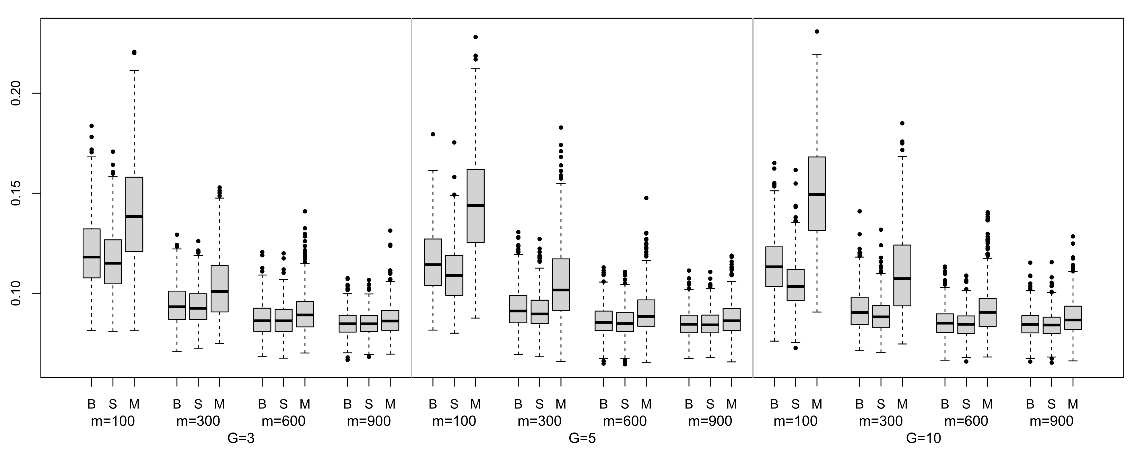
Additionally, we studied the median absolute prediction errors (MAE) of the ensemble methods under study for this data set. Figure 4 contains the box plots of the MAE distributions computed from 500 runs in each scenario. Most of the distributions are rightly skewed, with the exception of magging for m = 100 ; In general, magging takes greater median values than bagging or stacking and these differences are even greater for m = 100 . Summing up, it seems that the best performance is attained by stacking, although as m increases, the differences between stacking and bagging tend to decrease.
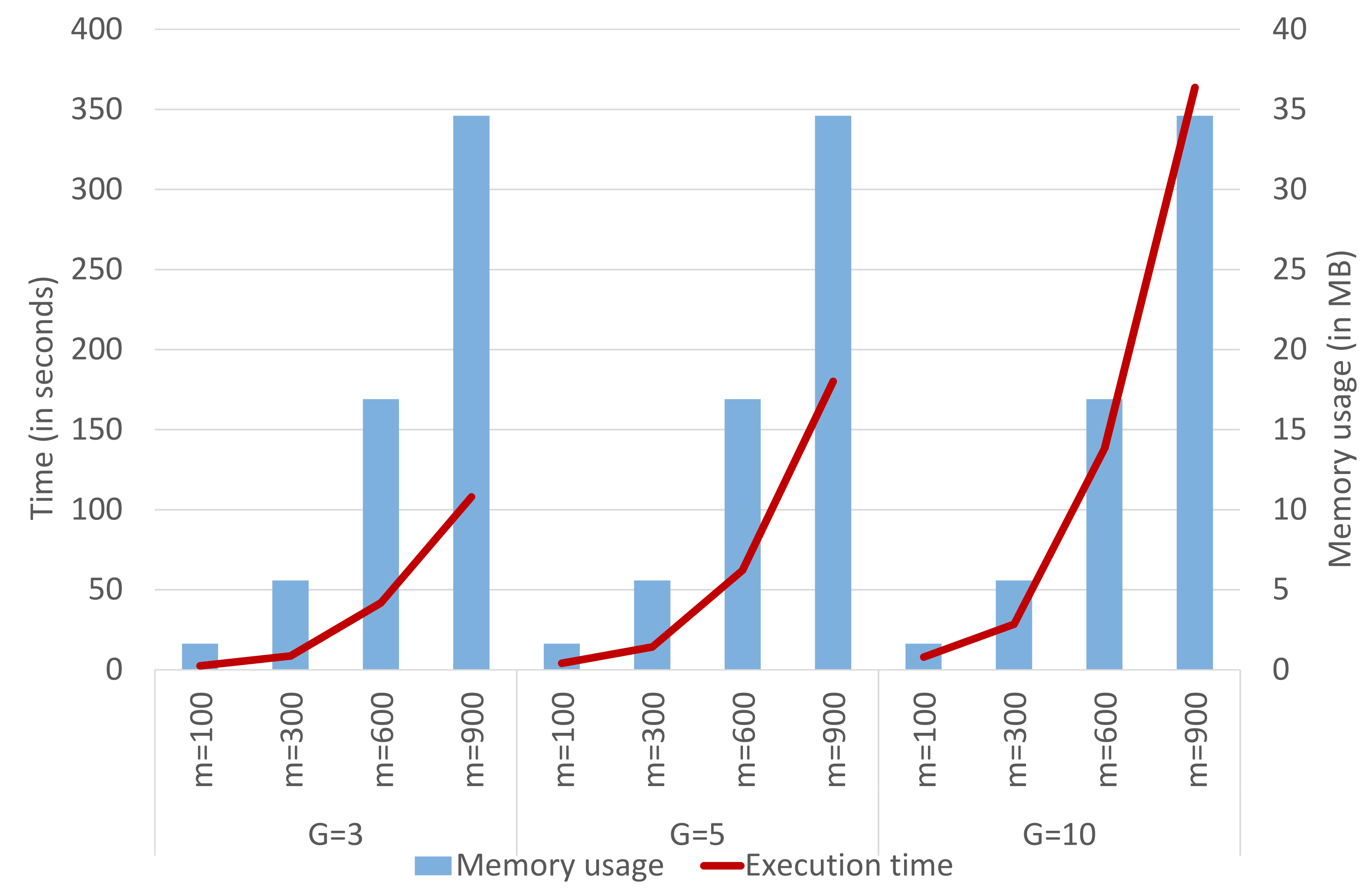
Finally, we analyze the complexity reduction, in terms of execution time and memory usage, when applying an ensemble technique to the DB-LM prediction model. Thus, we focus on the following R-functions, which are the actual bottlenecks of the computation process: daisy, disttoD2, and 
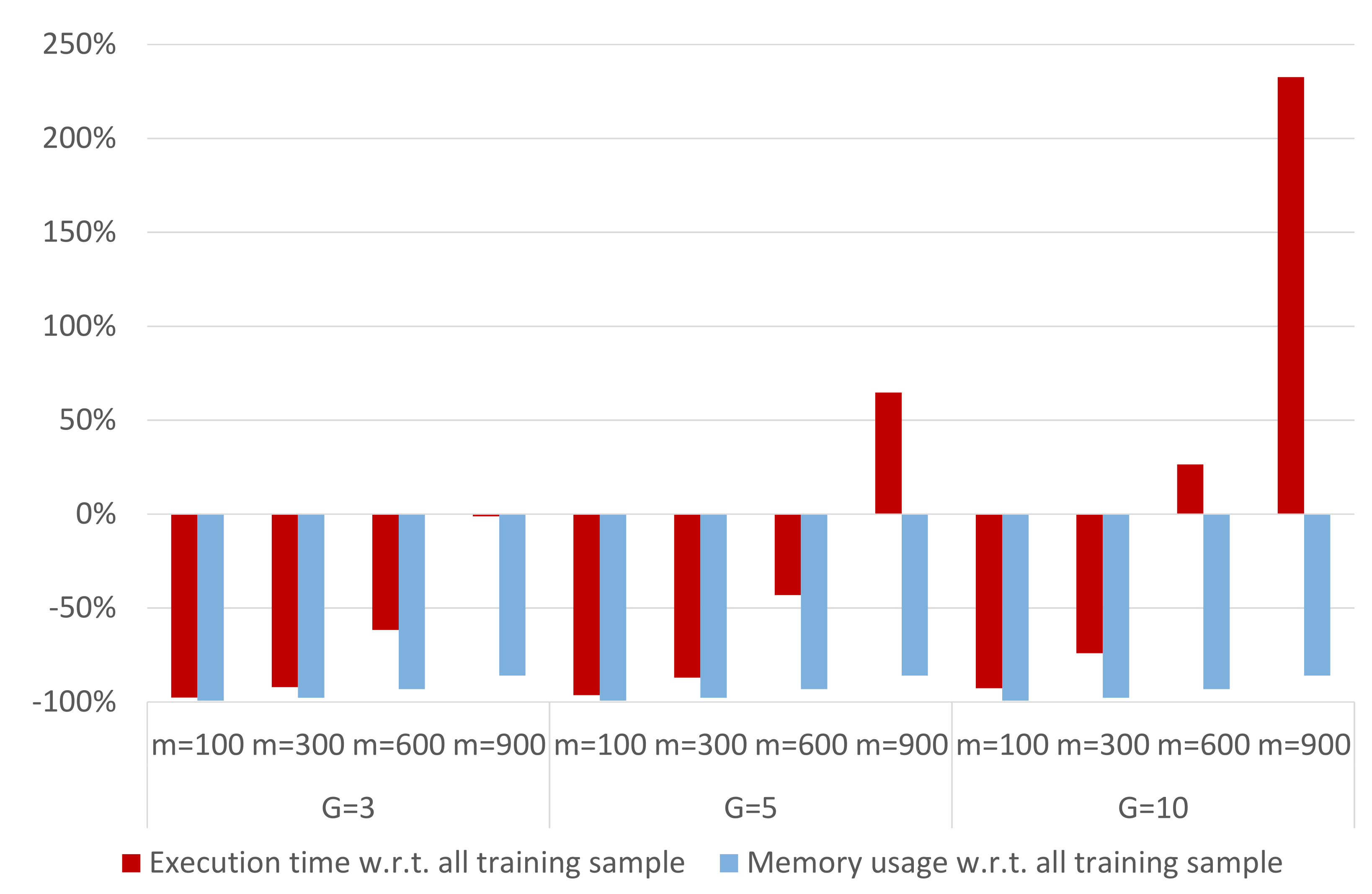
dblm. For the Capital Bikeshare data, DB-LM takes 109.35 s and occupies 247.3 MB when predicting 290 new cases based on a training sample of 2903 observations. On the other hand, the LM model takes 0.03 s to make these predictions and uses 1 MB of memory. DB-LM execution times and memory usage can considerably be reduced when applying any of the ensemble methods studied (in fact, they take 0 s in the optimization and averaging procedures for the predictions, which is why the execution time refers only to the three R-functions mentioned above). This can be seen in Figure 5, where we analyze the complexity of the ensemble DB-LM prediction model. We observe that the memory usage increases with m, although it remains constant with G. The execution time increases with m and G. These findings reinforce our conclusion that, for  G = 3 and m = 600 , the ensemble DB-LM prediction model provides a solution to the scalability problem, since the complexity of the DB-LM prediction model is considerably reduced and MSE is very close to that of the DB-LM (see Figure 3 and Figure 6).

3.1.2. King County House Sales

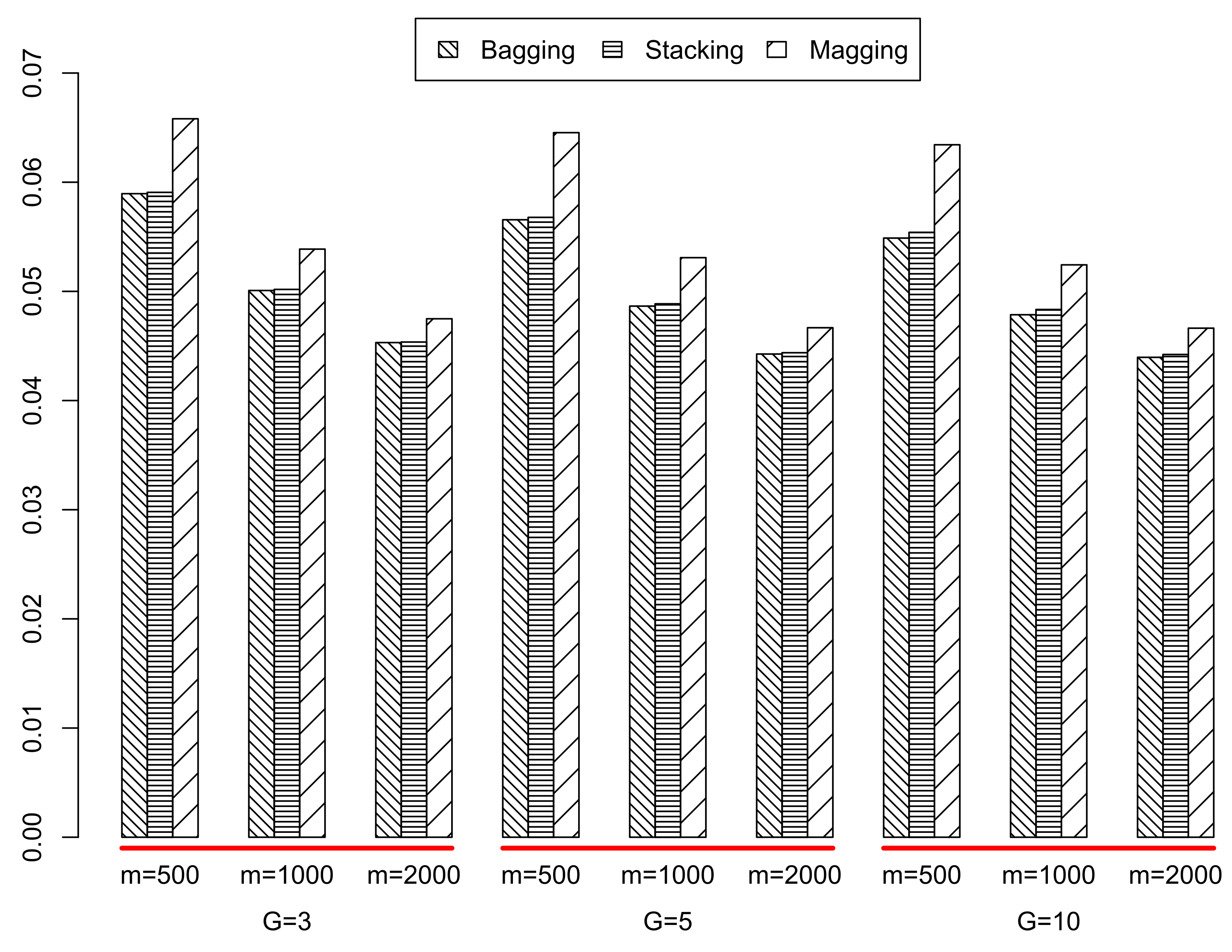
In each run of the Monte Carlo experiment, the whole sample was randomly divided into a test sample of 2159 individuals and a training sample of size n = 19,435. The number G of subsamples used was again 3, 5, and 10, and the values for the subsample size were m = 500 , 1000, and 2000. Given the large value of n, in this case it was not possible to perform DB regression on the whole training sample. Consequently, we report the average and standard deviation of the mean squared error attained with the ensemble procedures applied to DB-LM. In Table 6 and Table 7 and Figure 7, we display these results. For standard linear regression (using all the training information but only the quantitative predictors), the MSE was 0.10093, and with random forests (with 100 trees, mtry = 10, depth = 20) it was 0.04704.
In Table 8, we provide the p-values of the two-sided paired-sample Wilcoxon tests (with Bonferroni correction) conducted to compare the performance of the three ensemble methods for the King County sales data. As before, we evaluated the performance of each method with the MSE distribution computed from 500 runs within each scenario. The results confirm that all methods are significantly different in all cases. The results support even more the conclusions of Section 3.1.1. In this case, the best performing method is always bagging, although the results of stacking are almost identical. However, since the optimization inherent to stacking increases complexity as the sample size increases, again we strongly recommend the use of bagging in this framework of DB regression. Magging does not perform as well as bagging or stacking, even for the largest values of G and m. Larger values of m for stacking or magging were impossible to handle in the several, different computing resources we used (see Acknowledgements), even when dividing the Monte Carlo experiment in batches of 50 runs.
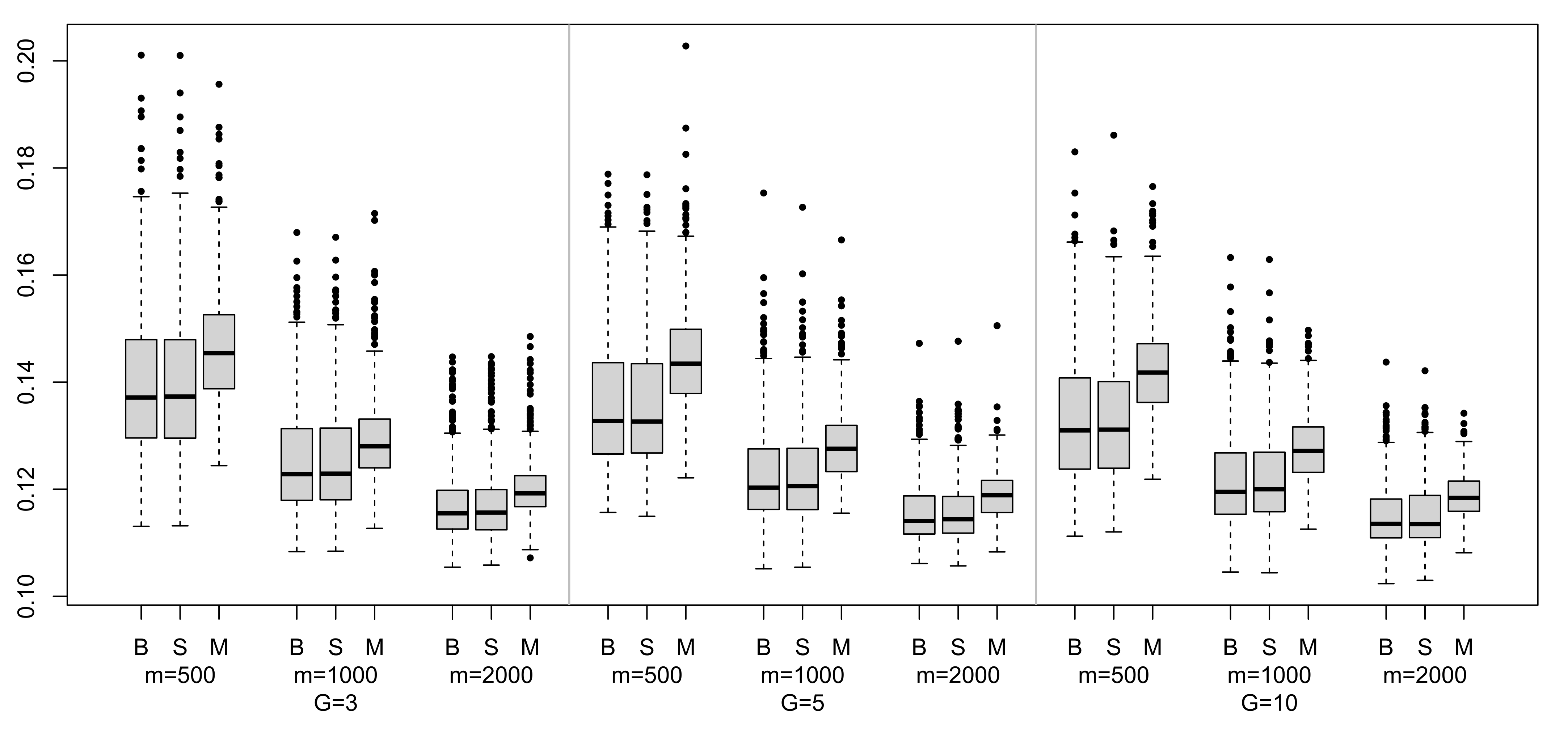
As before, we studied the MAE of the ensemble methods under study for this second data set. Figure 8 contains the box-plots of the MAE distributions computed from 500 runs in each scenario. We observe that all of them are rightly skewed distributions and that magging always takes greater median values than bagging or stacking, which seem to have a very similar distribution.

3.2. Bagging and DB-GLM: A Simulation Study

As a first example to illustrate the performance of the ensemble DB classifier, we analyzed the Online Shoppers Purchasing Intentiondataset from the UCI Machine Learning Repository (see [27]). The dataset consists of 12,330 e-shopping sessions, of which 10,422 did not end up with a purchase and the other 1908 ended up with shopping. There are 10 numerical and 8 qualitative attributes of each session (such as the month, operating system, browser, and region). We carried out a preliminary study where n = 2000 observations were randomly selected (without replacement) from the whole dataset. In each of 100 iterations, we separated this smaller sample into a training sample of 1800 observations and a test sample of size 200. The training sample was used to fit (i) the classical GLM model with only quantitative features, (ii) the DB-GLM using all the training sample, and (iii) the DB-GLM on G = 5 subsamples of size m = 400 , later aggregated using bagging. In all those situations, logit and probit link functions were considered. We used these six classifiers to allocate the observations in the test sample. However, the correct classification proportion was around 88% in all cases (see Table 9), meaning that bagging applied to DB-GLM performed just as well as DB-GLM on the whole sample, but also that the qualitative predictors were not informative enough to improve over the classical logistic model regardless of the link function used.
In order to control the proportion of different types of variables in the mixed data set as well as the a priori probability of the classes, and with the purpose of obtaining different scenarios to illustrate the performance of the procedures, we resorted to simulating mixed-type features from two populations using the R package Umpire (Coombes et al., 2021 [28]). In all cases, we sampled n “vectors” Z of 20 mixed-type features, with prior probabilities of the populations sampled from a Dirichlet distribution. We consider two models:
  • Model 1: The same proportion (1/3) of continuous, binary and nominal features.
  • Model 2: The proportion of continuous and binary features is the same (25% approximately), and the remaining (50%) of the features are qualitative ones.
In this context, we recall that nominal or qualitative refers to a variable with three or more possible values. The parameter values for the Clinical Noise Model in Umpire were shape = 1 and scale = 0.05. In each simulation experiment the sample of size n is simulated only once, and, from then on, these observations are treated as if they were one of the real data sets analyzed in Section 3.1.
We carried out two types of simulation studies. The first one was similar to the experiment with the Online Shoppers dataset described previously in this section. The aim was to check whether bagging applied to DB-GLM provided a good approximation to the correct classification rates of DB logistic regression fitted to the whole training sample. This has to be carried out on a relatively small training sample, since the fitting of a DB logistic regression model is computationally demanding. Based on our own experience, we chose a training sample of size 1800, for which the DB-GLM fitting took 1 hour with an Intel(R) Core(TM) i7-6700K CPU at 4.00 GHz and 32 GB RAM. Under these same conditions, the procedure was not feasible with a training sample size larger than 2000. The results in Section 3.1 show that bagging performs well when G × m is approximately equal to the whole sample size, so we chose G = 4 and m = 500 . The training and the test sample were sampled without replacement in each of the 100 iterations. Table 10 shows the overall correct classification proportions for Model 2 with the same three classifiers (with the logit link) used in the Online Shoppers data set analysis and a test sample size of 200 (that is, n = 1800 + 200 = 2000 ). The sample proportions of the two populations were 56% and 44%, and the number of continuous, binary, and nominal variables were 5, 5, and 10, respectively. The conclusion regarding bagging is the same as with the Online Shoppers data set and the regressions in Section 3.1: the subsampling and aggregation procedure performs just as well as using the whole sample, but the computing time is drastically reduced. Regarding logistic regression with just the quantitative features, we see that DB logistic regression attains a lower error rate, due to the incorporation of the nominal (informative) features into the model.
In the second simulation study, we sampled n = 10,000 observations from Models 1 and 2. In each of the 100 runs, the sample is split into a training sample of size 8000 and a test sample of size 2000. We fit two models: the logistic regression with only quantitative features and the DB logistic regression model on G = 20 subsamples of size m = 500 plus bagging. Table 11 displays the correct classification rates attained. The combination of bagging and DB logistic regression improves in both cases the correct classification rates of the classical logistic regression. The fact that the error proportions are lower in Model 2 than in Model 1 for both classifiers is only due to the effect of the specific sample simulated at the start of each Monte Carlo procedure.

4. Discussion

Distance-based regression is a technique able to deal with very general types of regressors or features, as long as a suitable dissimilarity is defined between them. The DB-LM and DB-GLM improve the performance of linear and generalized linear regression approaches, respectively, when qualitative predictors are available and informative about the response. Fitting the DB regression model is, however, computationally demanding, and the procedure is unfeasible when sample sizes are too large. Ensemble techniques provide a way of adapting DB regression to the analysis of large data sets. For medium sample sizes, we checked that subsampling and aggregation techniques (bagging, stacking, and magging) applied to DB linear regression attain the same error rates as DB-LM applied to the whole sample but reduce drastically the computing time. This conclusion also holds for bagging and DB logistic regression. Further, we have shown that these ensemble techniques allow the use of DB prediction models with large sample sizes, where the fitting to the global sample is out of reach but the use of qualitative predictors can contribute to improving the prediction or classification performance. Moreover, they appear to be competitive with state-of-the-art machine learning approaches, such as random forests, in regression tasks.

Author Contributions

Conceptualization, A.B. and A.G.; methodology, A.B. and A.G.; software, A.B. and A.G.; validation, A.B. and A.G.; formal analysis, A.B. and A.G.; investigation, A.B. and A.G.; resources, A.B. and A.G.; data curation, A.B. and A.G.; writing—original draft preparation, A.B. and A.G.; writing—review and editing, A.B. and A.G.; visualization, A.B. and A.G.; supervision, A.B. and A.G.; project administration, A.B. and A.G.; funding acquisition, A.B. and A.G. All authors have read and agreed to the published version of the manuscript.

Funding

A. Baíllo is supported by the Spanish MCyT grant PID2019-109387GB-I00.

Institutional Review Board Statement

Not applicable.

Informed Consent Statement

Not applicable.

Acknowledgments

The computation leading to the results in this work was carried out in parallel in the Center for Scientific Computing at Universidad Autónoma de Madrid and in the computers of several kind colleagues: A. Arribas (UC3M), J.R. Berrendero (UAM), A. Cuevas (UAM), and J.L. Torrecilla (UAM). We thank every one of them for their generous collaboration. We thank the anonymous reviewers for their comments, leading to an improved version of the manuscript.

Conflicts of Interest

The authors declare no conflict of interest. The funders had no role in the design of the study; in the collection, analyses, or interpretation of data; in the writing of the manuscript; or in the decision to publish the results.

References

  1. Boj, E.; Delicado, P.; Fortiana, J. Local linear functional regression based on weighted distance—Based regression. Comput. Stat. Data Ananl. 2010, 54, 429–437. [Google Scholar] [CrossRef]
  2. Wang, R.; Shan, S.; Chen, X.; Dai, Q.; Gao, W. Manifold–manifold distance and its application to face recognition with image sets. IEEE Trans. Image Process. 2012, 21, 4466–4479. [Google Scholar] [CrossRef]
  3. Shao, M.-W.; Du, X.-J.; Wang, J.; Zhai, C.-M. Recognition of leaf image set based on manifold-manifold distance. In International Conference on Intelligent Computing (ICIC) 2014; Lecture Notes in Computer Science; Springer: Taiyuan, China, 2014; pp. 332–337. [Google Scholar]
  4. Tsitsulin, A.; Munkhoeva, M.; Mottin, D.; Karras, P.; Bronstein, A.; Oseledets, I.; Müller, E. The Shape of Data: Intrinsic Distance for Data Distributions. 2020. Available online: https://arxiv.org/abs/1905.11141 (accessed on 30 August 2021).
  5. Cuadras, C.M. Distance analysis in discrimination and classification using both continuous and categorical variables. In Statistical Data Analysis and Inference; Dodge, Y., Ed.; North-Holland Publishing Co.: Amsterdam, The Netherlands, 1989; pp. 459–473. [Google Scholar]
  6. Cuadras, C.M.; Arenas, C. A distance-based model for prediction with mixed data. Commun. Stat. Theory Methods 1990, 19, 2261–2279. [Google Scholar] [CrossRef]
  7. Cuadras, C.M.; Arenas, C.; Fortiana, J. Some computational aspects of a distance-based model for prediction. Commun. Stat. Simul. Comput. 1996, 25, 593–609. [Google Scholar] [CrossRef]
  8. Boj, E.; Caballé, A.; Delicado, P.; Esteve, A.; Fortiana, J. Global and local distance-based generalized linear models. Test 2016, 25, 170–195. [Google Scholar] [CrossRef] [Green Version]
  9. Mendes-Moreira, J.; Soares, C.; Jorge, A.M.; de Sousa, J.F. Ensemble approaches for regression: A survey. ACM Comput. Surv. 2012, 45, 10. [Google Scholar] [CrossRef]
  10. Ren, Y.; Zhang, L.; Suganthan, P.N. Ensemble classification and regression—Recent developments, applications and future directions. IEEE Comput. Intell. Mag. 2016, 11, 41–53. [Google Scholar] [CrossRef]
  11. Breiman, L. Bagging predictors. Mach. Learn. 1996, 24, 123–140. [Google Scholar] [CrossRef] [Green Version]
  12. Breiman, L. Stacked regressions. Mach. Learn. 1996, 24, 49–64. [Google Scholar] [CrossRef] [Green Version]
  13. Bühlmann, P. Bagging, subagging and bragging for improving some prediction algorithms. In Recent Advances and Trends in Nonparametric Statistics; Elsevier: Amsterdam, The Netherlands, 2003; pp. 19–34. [Google Scholar]
  14. Bühlmann, P.; Meinshausen, N. Magging: Maximin aggregation for inhomogeneous large-scale data. Proc. IEEE 2015, 104, 126–135. [Google Scholar] [CrossRef] [Green Version]
  15. McCullagh, P.; Nelder, J.A. Generalized Linear Models; Chapman and Hall: London, UK, 1989. [Google Scholar]
  16. Boj, E.; Caballé, A.; Delicado, P.; Fortiana, J. Dbstats: Distance-Based Statistics. R Package, Version 1.0.5. 2017. Available online: https://CRAN.R-project.org/package=dbstats (accessed on 3 June 2019).
  17. Gower, J.C. Adding a point to vector diagrams in multivariate analysis. Biometrika 1968, 55, 582–585. [Google Scholar] [CrossRef]
  18. De Leon, A.R.; Soo, A.; Williamson, T. Classification with discrete and continuous variables via general mixed-data models. J. Appl. Stat. 2011, 38, 1021–1032. [Google Scholar] [CrossRef]
  19. Gower, J.C. A general coefficient of similarity and some of its properties. Biometrics 1971, 27, 857–874. [Google Scholar] [CrossRef]
  20. Grané, A.; Salini, S.; Verdolini, E. Robust multivariate analysis for mixed-type data: Novel algorithm and its practical application in socio-Economic research. Socio-Econ. Plan. Sci. 2021, 73, 100907. [Google Scholar] [CrossRef]
  21. Paradis, E. Multidimensional scaling with very large datasets. J. Comput. Graph. Stat. 2018, 27, 935–939. [Google Scholar] [CrossRef]
  22. Grané, A.; Sow-Barry, A.A. Visualizing profiles of large datasets of weighted and mixed data. Mathematics 2021, 9, 891. [Google Scholar] [CrossRef]
  23. Zhu, M. Use of majority votes in statistical learning. WIREs Comput. Stat. 2015, 7, 357–371. [Google Scholar] [CrossRef]
  24. Wolpert, D. Stacked generalization. Neural Netw. 1992, 5, 241–259. [Google Scholar] [CrossRef]
  25. Džeroski, S.; Ženko, B. Is combining classifiers with stacking better than selecting the best one? Mach. Learn. 2004, 54, 255–273. [Google Scholar] [CrossRef] [Green Version]
  26. Meinshausen, N.; Bühlmann, P. Maximin effects in inhomogeneous large-scale data. Ann. Stat. 2015, 43, 1801–1830. [Google Scholar] [CrossRef] [Green Version]
  27. Sakar, C.O.; Polat, S.O.; Katircioglu, M.; Kastro, Y. Real-time prediction of online shoppers’ purchasing intention using multilayer perceptron and LSTM recurrent neural networks. Neural Comput. Appl. 2018, 31, 6893–6908. [Google Scholar] [CrossRef]
  28. Coombes, C.E.; Abrams, Z.B.; Nakayiza, S.; Brock, G.; Coombes, K.R. Umpire 2.0: Simulating realistic, mixed–type, clinical data for machine learning. F1000Research 2021, 9, 1186. [Google Scholar] [CrossRef]
Figure 1. Flowchart for the ensemble (bagging, stacking, or magging) DB prediction.
Mathematics 09 02247 g001
Figure 2. Block diagram for the DB-LM prediction.
Mathematics 09 02247 g002
Figure 3. Mean squared prediction errors for the Capital Bikeshare data.
Mathematics 09 02247 g003
Figure 4. Box-plots for the median absolute prediction errors (MAE) for the Capital Bikeshare data. For each method, the performance is evaluated with the distribution of MAE values computed in 500 runs within each scenario.
Mathematics 09 02247 g004
Figure 5. Complexity analysis (execution time and memory usage) of the ensemble DB-LM prediction model for the Capital Bikeshare data.
Mathematics 09 02247 g005
Figure 6. Percentage of complexity reduction of the ensemble DB-LM prediction model for the Capital Bikeshare data. Baseline: Execution time of 109.35 s and memory usage of 243.3 MB to predict 290 new cases using all the training sample.
Mathematics 09 02247 g006
Figure 7. Mean squared prediction errors for the King County house sales data.
Mathematics 09 02247 g007
Figure 8. Box plots for the median absolute prediction errors (MAE) for the King County house sales data.
Mathematics 09 02247 g008
Table 1. Variables included in the bikes dataset.
Capital Bikeshare
Total count of daily users (both registered and not)
Season: winter (1), spring (2), summer (3), autumn (4)
Year, codified to 0 (=2011), 1 (=2012), 2 (=2013), …, 7 (=2018)
Month, codified to 1, 2, …, 12
National holiday (1) or not (0)
Weekday, codified to 0 (=Sunday), 1 (=Monday), …, 6 (=Saturday)
Working day (1) or weekend day (0)
NOAA at DCA
Average daily wind speed (miles per hour)
Precipitation (inches to hundredths)
Maximum temperature (in Fahrenheit)
Minimum temperature (in Fahrenheit)
Ceiling height dimension (in meters)
Mean daily temperature (in Celsius)
Sea level pressure (in hPa)
Relative humidity (in %)
Table 2. Variables in King County house sales data.
dateDate of the home sale
pricePrice of each home sold
bedroomsNumber of bedrooms
bathroomsNumber of bathrooms
sqft_livingSquare footage (sqft) of the interior living space
sqft_lotSqft of the land space
floorsNumber of floors
waterfront1 if the house overlooks the waterfront; 0 if not
viewIndex from 0 to 4 grading the view from the property
conditionIndex from 1 to 5 on the condition of the house
gradeIndex from 1 to 13, grading quality of construction and design
sqft_aboveSqft of the interior housing space above ground level
sqft_basementSqft of the interior housing space below ground level
yr_builtThe year the house was initially built
yr_renovatedThe year of the house’s last renovation
zipcodeZipcode area the house is in
latLatitude
longLongitude
sqft_living15Sqft of interior living space for the nearest 15 neighbors
sqft_lot15Sqft of the land lots of the nearest 15 neighbors
Table 3. Average (standard deviation) of mean squared prediction errors (MSE) for the Capital Bikeshare data with the ensemble procedures. Summary statistics computed across 500 iterations.
GmBaggingStackingMagging
31000.03303 (0.005855)0.03223 (0.005579)0.04217 (0.010301)
33000.02445 (0.003641)0.02424 (0.003559)0.02740 (0.005098)
36000.02257 (0.003102)0.02251 (0.003080)0.02365 (0.003562)
39000.02226 (0.003052)0.02224 (0.003046)0.02278 (0.003216)
51000.03064 (0.005142)0.02940 (0.004556)0.04323 (0.010627)
53000.02381 (0.003535)0.02349 (0.003360)0.02793 (0.005720)
56000.02223 (0.002936)0.02216 (0.002902)0.02352 (0.003551)
59000.02185 (0.003004)0.02182 (0.002997)0.02246 (0.003151)
101000.02958 (0.004680)0.02779 (0.004059)0.04471 (0.010182)
103000.02360 (0.003440)0.02307 (0.003197)0.02909 (0.006110)
106000.02221 (0.003054)0.02207 (0.003012)0.02399 (0.003898)
109000.02187 (0.002960)0.02181 (0.002947)0.02268 (0.003196)
Table 4. m and G m as percentages of the training sample size n = 2613 .
m m as % of n G m as % of n
G
3510
1004%11%19%38%
30011%34%57%115%
60023%69%115%230%
90034%103%172%344%
Table 5. Results of the two-sided paired-sample Wilcoxon tests (with Bonferroni correction) for in Capital Bikesharing data.
m = 100 m = 300
B-SB-MS-MB-SB-MS-M
G = 3 ******************
G = 5 ******************
G = 10 ******************
m = 600 m = 900
B-SB-MS-MB-SB-MS-M
G = 3 3.91 × 10 15 ****** 1.16 × 10 4 ******
G = 5 2.75 × 10 12 ****** 8.49 × 10 8 ******
G = 10 ********* 3.91 × 10 13 ******
*** p-value lower than 6.6 × 10 16 .
Table 6. Average (standard deviation) in prediction of the logarithm of sale price in King County houses data with the ensemble procedures. Summary statistics computed across 500 iterations.
GmBaggingStackingMagging
35000.05895 (0.00817)0.05907 (0.00811)0.06581 (0.00804)
310000.05008 (0.00602)0.05018 (0.00600)0.05387 (0.00598)
320000.04531 (0.00390)0.04536 (0.00392)0.04749 (0.00362)
55000.05656 (0.00756)0.05678 (0.00744)0.06454 (0.00794)
510000.04865 (0.00547)0.04886 (0.00548)0.05309 (0.00509)
520000.04426 (0.00343)0.04438 (0.00348)0.04667 (0.00312)
105000.05488 (0.00717)0.05540 (0.00699)0.06343 (0.00717)
1010000.04786 (0.00514)0.04834 (0.00523)0.05243 (0.00445)
1020000.04396 (0.00344)0.04422 (0.00357)0.04663 (0.00297)
Table 7. m and G m as percentages of the training sample size n = 19,435.
m m as % of n G m as % of n
G
3510
5003%8%13%26%
10005%15%26%51%
200010%31%51%103%
Table 8. Results of the two-sided paired-sample Wilcoxon tests (with Bonferroni correction) for King County house sales data.
m = 500 m = 1000 m = 2000
B-SB-MS-MB-SB-MS-MB-SB-MS-M
G = 3 1.72 × 10 11 ************************
G = 5 1.98 × 10 15 ************************
G = 10 ***************************
*** p-value lower than 6.6 × 10 16 .
Table 9. Correct classification rates for Online Shoppers with n = 2000 .
Link FunctionClassical GLM (Quantitative Features)DB-GLM (Whole Sample)DB-GLM and Bagging
logit0.889400.883800.88395
probit0.889300.884650.88350
Table 10. Correct classification rates for Model 2 with n = 2000 .
Classical Logistic (Quantitative Features)DB Logistic (Whole Sample)DB Logistic and Bagging
0.74010.97340.9780
Table 11. Correct classification rates for Models 1 and 2 with n = 10,000 .
Classical Logistic (Quantitative Features)DB Logistic and Bagging
Model 10.82200.9244
Model 20.92080.9601
Publisher’s Note: MDPI stays neutral with regard to jurisdictional claims in published maps and institutional affiliations.

