Structure Identification of Fractional-Order Dynamical Network with Different Orders

Abstract

Topology structure and system parameters have a great influence on the dynamical behavior of dynamical networks. However, they are sometimes unknown or uncertain in advance. How to effectively identify them has been investigated in various network models, from integer-order networks to fractional-order networks with the same order. In the real world, many systems consist of subsystems with different fractional orders. Therefore, the structure identification of a dynamical network with different fractional orders is investigated in this paper. Through designing proper adaptive controllers and parameter updating laws, two network estimators are well constructed. One is for identifying only the unknown topology structure. The other is for identifying both the unknown topology structure and system parameters. Based on the Lyapunov function method and the stability theory of fractional-order dynamical systems, the theoretical results are analytically proved. The effectiveness is verified by three numerical examples as well. In addition, the designed estimators have a good performance in monitoring switching topology. From the practical viewpoint, the designed estimators can be used to monitor the change of current and voltage in the fractional-order circuit systems.

1. Introduction

Topology structure and system parameters, as we know, play a great role in many studies on dynamical networks. In pinning control, as a specific example, how to choose the pinned nodes is usually based on the node degree calculated from the topology structure. In practical applications, however, the topology structure and system parameters of dynamical networks may be unknown or partially unknown. In cellular networks, for instance, the interactions among the protein-DNAs, described by the topological structure, are sometimes unknown. Since the DNA interactions have a great effect on cellular processes, how to effectively identify them is an interesting and important issue and deserves deep study. Thus far, researchers have performed much research on the structure identification issue of dynamical networks [1,2,3,4,5,6,7,8,9,10,11,12,13,14,15]. In [15], Waarde et al. addressed the problem of identifying the graph structure of a dynamical network using measured input/output data. In [9], Ding et al. investigated the topology identification problem for power systems. In [10], Farajollahi et al. investigated the topology identification problem for distribution systems. It is noted that the studies on structure identification of dynamical networks have potential applications in real systems.

Recently, the fractional-order calculus, as an extension of the integer-order calculus, has received increasing attention since it has some good properties (such as the infinite memory and genetic characteristics) and more degrees of freedom compared with the integer-order calculus [16,17]. That is, the fractional dynamical networks can more precisely describe the characteristics of physical systems. Nowadays, many valuable results about the fractional-order networks have been obtained [18,19,20,21,22,23,24,25]. In [18], Si et al. gave the sufficient condition of structure identification in uncertain fractional dynamical networks, and further discussed the effects of coupling strength and fractional order on the identification process. In [21], Du investigated the parameters identification issue of fractional dynamical networks by achieving the modified function projective synchronization between the drive-response networks.

It is worth noting that the networks in the aforementioned literature [18,19,20,21,22,23,24,25,26,27,28] are formed by many coupled subsystems with the same fractional order. In fact, complex networks may consist of subsystems with different fractional orders in the real world. In [29], Kaczorek used fractional-order current and voltage equations with different orders to describe the linear circuits. In [30], Datsko et al. studied fractional reaction-diffusion systems, in which the derivative order of activator and inhibitor variables are different. Naturally, how to identify the unknown topology structure of a dynamical network with different fractional orders is a challenging issue and deserves further study.

Motivated by the above discussions, this paper investigates the structure identification of a fractional-order dynamical network with different orders. The main contribution is to design network estimators based on the adaptive feedback control method and parameter updating laws in two cases: (i) assume that only the topology is unknown and to be identified; (ii) assume that both the topology and system parameters are unknown.

The rest of this paper is organized as follows. In Section 2, the fractional-order complex network model is introduced, and some necessary definitions, assumptions and lemmas are given. In Section 3, two corresponding effective estimators are designed. In Section 4, numerical examples are performed to verify the correctness and effectiveness of the theoretical results. Finally, the conclusions are drawn in Section 5.

2. Model Description and Preliminaries

Throughout this paper, the fractional-order calculus is Caputo calculus. In the following, some basic definitions and lemmas about Caputo calculus are presented.

Definition 1

([16]). The fractional integral of order α for function $f\left(t\right)$ is defined as:

$$\begin{array}{c}\hfill D_{t_0,t}^{-\alpha }f\left(t\right)=\frac{1}{\Gamma \left(\alpha \right)}{\int }_{t_0}^t{(t-\tau )}^{\alpha -1}f\left(\tau \right)\mathrm{d}\tau ,\end{array}$$

where $t\ge t_0$, $\alpha >0$, and $\Gamma (·)$ is the Gamma function.

Definition 2

([16]). The α-$th$-$order$ Caputo fractional derivative of the given function $f\left(t\right)$ is defined as:

$$\begin{array}{c}\hfill {}_C{D}_{t_0,t}^{\alpha }f\left(t\right)=\frac{1}{\Gamma (m-\alpha )}{\int }_{t_0}^t{(t-\tau )}^{m-\alpha -1}{f}^{\left(m\right)}\left(\tau \right)\mathrm{d}\tau ,\end{array}$$

where $m-1<\alpha <m$, $m\in {\mathbb{Z}}^{+}$.

In general, the initial time $t_0$ is often considers as $t_0=0$. Then, for the sake of simplicity, the $D_{0,t}^{-\alpha }$ is denoted by $D^{-\alpha }$ and ${}_C{D}_{0,t}^{\alpha }$ by $D^{\alpha }$.

Lemma 1

([31]). If $x\left(t\right),z\left(t\right)\in C^1\left[t_0,b\right]$, and $\alpha >0,\beta >0$, then

$$\begin{array}{cc}\hfill & \left(1\right)D^{\alpha }{D}^{-\beta }x\left(t\right)=D^{\alpha -\beta }x\left(t\right),\hfill \\ \hfill & \left(2\right)D^{\alpha }\left(x\left(t\right)\pm z\left(t\right)\right)=D^{\alpha }x\left(t\right)\pm D^{\alpha }z\left(t\right).\hfill \end{array}$$

Lemma 2

([32]). Let $x\left(t\right)\in {\mathbb{R}}^n$ be a differentiable vector function. Then, for any time instant $t\ge 0$

$$\begin{array}{c}\hfill \frac{1}{2}{D}^{\alpha }\left(x^T\left(t\right)x\left(t\right)\right)\le x^T\left(t\right)\left(D^{\alpha }x\left(t\right)\right),\end{array}$$

where $\alpha \in (0,1)$ is the fractional order.

Consider the following fractional-order dynamical network

$$\begin{array}{c}\hfill D^{{\alpha }_i}{y}_i\left(t\right)=f_i(y_i\left(t\right),{\varphi }_i)+c\sum _{j=1}^N{a}_{ij}H{y}_j\left(t\right),i=1,2,\cdots ,N,\end{array}$$

(1)

where $0<{\alpha }_i<1$, $y_i\left(t\right)={(y_{i1}\left(t\right),y_{i2}\left(t\right),\cdots ,y_{in}\left(t\right))}^T\in {\mathbb{R}}^n$ is the state vector of the ith node, $f_i$ is a continuous and differentiable vector function, ${\varphi }_i\in {\mathbb{R}}^{q_i}$ is a parameter vector, $c>0$ is the coupling strength, $H=diag(h_1,h_2,\cdots ,h_n)$ is the inner coupling matrix, $A=\left(a_{ij}\right)\in {\mathbb{R}}^{N\times N}$ is the zero-row-sum outer coupling matrix, defined as: if there is a connection from node j to node i, then $a_{ij}\ne 0(i\ne j)$ ; otherwise, $a_{ij}=0$.

In this paper, $f_i$ is assumed to be a linear function about ${\varphi }_i$, namely

$$\begin{array}{c}\hfill f_i(y_i\left(t\right),{\varphi }_i)=g_i\left(y_i\left(t\right)\right)+G_i\left(y_i\left(t\right)\right){\varphi }_i.\end{array}$$

(2)

Assumption 1.

Suppose that there exists a positive definite matrix Δ such that

$$\begin{array}{c}\hfill {(\widehat{y}-y)}^T\left(f_i(\widehat{y},{\varphi }_i)-f_i(y,{\varphi }_i)\right)\le {(\widehat{y}-y)}^T\Delta (\widehat{y}-y)\end{array}$$

(3)

for any $\widehat{y},y\in {\mathbb{R}}^n$ and $i=1,2,\cdots ,N$, where $\Delta =diag({\delta }_1,{\delta }_2,\cdots ,{\delta }_n)$.

Assumption 2.

Denote $G_i\left(y_i\right)=\left(G_i^1\left(y_i\right),\cdots ,G_i^{q_i}\left(y_i\right)\right)$. Suppose that ${\{{\left\{G_i^k\left(y_i\right)\right\}}_{k=1}^{q_i},H{y}_i\}}_{i=1}^N$ are linearly independent on the orbits ${\left\{y_i\left(t\right)\right\}}_{i=1}^N$ for $t>0$.

3. Main Results

Firstly, assume that only the topology is unknown. The network estimator is designed as

$$\begin{array}{c}\hfill D^{{\alpha }_i}{\widehat{y}}_i\left(t\right)=f_i({\widehat{y}}_i\left(t\right),{\varphi }_i)+c\sum _{j=1}^N{\widehat{a}}_{ij}\left(t\right)H{\widehat{y}}_j\left(t\right)+u_i\left(t\right),i=1,2,\cdots ,N,\end{array}$$

(4)

where $u_i\left(t\right)$ are controllers to be designed, $\widehat{A}\left(t\right)=\left({\widehat{a}}_{ij}\left(t\right)\right)\in {\mathbb{R}}^{N\times N}$ is the estimation of the unknown matrix A.

Define $e_i\left(t\right)={\widehat{y}}_i\left(t\right)-y_i\left(t\right)$, then the error system is

$$\begin{array}{cc}\hfill D^{{\alpha }_i}{e}_i\left(t\right)=& f_i({\widehat{y}}_i\left(t\right),{\varphi }_i)-f_i(y_i\left(t\right),{\varphi }_i)+c\sum _{j=1}^N{a}_{ij}H{e}_j\left(t\right)\hfill \\ \hfill & +c\sum _{j=1}^N({\widehat{a}}_{ij}\left(t\right)-a_{ij})H{\widehat{y}}_j\left(t\right)+u_i\left(t\right).\hfill \end{array}$$

(5)

Theorem 1.

Suppose that Assumptions 1 and 2 hold. Then the unknown matrix A of network (1) is identified by the $\widehat{A}\left(t\right)$ of network estimator (4) with the following adaptive controllers $u_i\left(t\right)$ and updated laws

$$\begin{array}{cc}\hfill u_i\left(t\right)& =-w\left(t\right)e_i\left(t\right),\hfill \\ \hfill D^{{\alpha }_0}w\left(t\right)& =\theta \sum _{i=1}^N{e}_i^T\left(t\right)e_i\left(t\right),\hfill \\ \hfill D^{{\alpha }_i}{\widehat{a}}_{ij}\left(t\right)& =-{\mu }_{ij}{\widehat{y}}_j^T\left(t\right)H{e}_i\left(t\right),\hfill \end{array}$$

(6)

where $i,j=1,2,\cdots ,N,\theta >0,{\mu }_{ij}>0$ are adaptive gains, and ${\alpha }_0={\displaystyle \underset{1\le k\le N}{max}}\left\{{\alpha }_k\right\}$.

Proof. 

Consider the following Lyapunov function:

$$\begin{array}{cc}\hfill V\left(t\right)=& \frac{1}{2}\sum _{i=1}^N{D}^{{\alpha }_i-{\alpha }_0}\left(e_i^T\left(\tau \right)e_i\left(\tau \right)\right)+\frac{1}{2\theta }{\left(w\left(t\right)-\widehat{w}\right)}^2\hfill \\ \hfill & +\sum _{i=1}^N\sum _{j=1}^N\frac{c}{2{\mu }_{ij}}{D}^{{\alpha }_i-{\alpha }_0}\left({({\widehat{a}}_{ij}\left(\tau \right)-a_{ij})}^2\right),\hfill \end{array}$$

(7)

where $\widehat{w}$ is a positive constant to be determined.

According to Lemmas 1 and 2, the derivative of $V\left(t\right)$ is calculated as

$$\begin{array}{cc}\hfill D^{{\alpha }_0}V\left(t\right)=& \sum _{i=1}^N{D}^{{\alpha }_i}\left(\frac{1}{2}{e}_i^T\left(t\right)e_i\left(t\right)\right)+\frac{1}{\theta }\left(w\left(t\right)-\widehat{w}\right)\left(D^{{\alpha }_0}w\left(t\right)\right)\hfill \\ \hfill & +\sum _{i=1}^N\sum _{j=1}^N\frac{c}{{\mu }_{ij}}({\widehat{a}}_{ij}\left(t\right)-a_{ij})\left(D^{{\alpha }_i}{\widehat{a}}_{ij}\left(t\right)\right)\hfill \\ \hfill \le & \sum _{i=1}^N{e}_i^T\left(t\right)\left(D^{{\alpha }_i}{e}_i\left(t\right)\right)+\frac{1}{\theta }\left(w\left(t\right)-\widehat{w}\right)\left(\theta \sum _{i=1}^N{e}_i^T\left(t\right)e_i\left(t\right)\right)\hfill \\ \hfill & +\sum _{i=1}^N\sum _{j=1}^N\frac{c}{{\mu }_{ij}}({\widehat{a}}_{ij}\left(t\right)-a_{ij})\left(-{\mu }_{ij}{\widehat{y}}_j^T\left(t\right)H{e}_i\left(t\right)\right)\hfill \\ \hfill =& \sum _{i=1}^N{e}_i^T\left(t\right)\left(f_i({\widehat{y}}_i\left(t\right),{\varphi }_i)-f_i(y_i\left(t\right),{\varphi }_i)\right)+c\sum _{i=1}^N\sum _{j=1}^N{a}_{ij}{e}_i^T\left(t\right)H{e}_j\left(t\right)\hfill \\ \hfill & +c\sum _{i=1}^N\sum _{j=1}^N\left({\widehat{a}}_{ij}\left(t\right)-a_{ij}\right)e_i^T\left(t\right)H{\widehat{y}}_j\left(t\right)-\sum _{i=1}^{N}w\left(t\right)e_i^T\left(t\right)e_i\left(t\right)\hfill \\ \hfill & +\left(w\left(t\right)-\widehat{w}\right)\sum _{i=1}^N{e}_i^T\left(t\right)e_i\left(t\right)-c\sum _{i=1}^N\sum _{j=1}^N\left({\widehat{a}}_{ij}\left(t\right)-a_{ij}\right){\widehat{y}}_j^T\left(t\right)H{e}_i\left(t\right)\hfill \\ \hfill =& \sum _{i=1}^N{e}_i^T\left(t\right)\left(f_i({\widehat{y}}_i\left(t\right),{\varphi }_i)-f_i(y_i\left(t\right),{\varphi }_i)\right)\hfill \\ \hfill & +c\sum _{i=1}^N\sum _{j=1}^N{a}_{ij}{e}_i^T\left(t\right)H{e}_j\left(t\right)-\widehat{w}\sum _{i=1}^N{e}_i^T\left(t\right)e_i\left(t\right)\hfill \\ \hfill \le & \sum _{i=1}^N{e}_i^T\left(t\right)\left(\Delta -\widehat{w}{I}_n\right)e_i\left(t\right)+c\sum _{i=1}^N\sum _{j=1}^N{a}_{ij}{e}_i^T\left(t\right)H{e}_j\left(t\right)\hfill \\ \hfill =& e^T\left(t\right)\left(I_N\otimes \Delta -\widehat{w}{I}_N\otimes I_n+c(A^s\otimes H)\right)e\left(t\right),\hfill \end{array}$$

where $e\left(t\right)={(e_1^T\left(t\right),e_2^T\left(t\right),\cdots ,e_N^T\left(t\right))}^T$, $A^s=(A+A^T)/2$, $I_n$ and $I_N$ are n- and N-dimensional identity matrices respectively, ‘⊗’ denotes the Kronecker product.

Let $\widehat{\delta }={\displaystyle \underset{1\le p\le N}{max}}\left\{{\delta }_p\right\}$, $\lambda$ be the largest eigenvalues of $A^s\otimes H$. Choose $\widehat{w}=\widehat{\delta }+c\lambda +1$, we obtain

$$D^{{\alpha }_0}V\left(t\right)\le -e^T\left(t\right)e\left(t\right).$$

(8)

Based on the Lyapunov stability theory, we have $e\left(t\right)\to 0$ as $t\to \infty$. Then rewrite (5) as

$$\sum _{j=1}^N({\widehat{a}}_{ij}\left(t\right)-a_{ij})H{y}_j\left(t\right)=0,i=1,2,\cdots ,N.$$

By Assumption 2, it is clear that ${\widehat{a}}_{ij}\left(t\right)\to a_{ij}$, i.e., the unknown A is identified. Thus the proof is completed. □

Secondly, assume that both topology and system parameters are unknown. The network estimator is designed as

$$\begin{array}{cc}\hfill D^{{\alpha }_i}{\widehat{y}}_i\left(t\right)=& g_i\left({\widehat{y}}_i\left(t\right)\right)+G_i\left({\widehat{y}}_i\left(t\right)\right){\phi }_i\left(t\right)+c\sum _{j=1}^N{\widehat{a}}_{ij}\left(t\right)H{\widehat{y}}_j\left(t\right)+u_i\left(t\right),\hfill \end{array}$$

(9)

where $i=1,2,\cdots ,N$, $\widehat{A}\left(t\right)=\left({\widehat{a}}_{ij}\left(t\right)\right)\in {\mathbb{R}}^{N\times N}$ and ${\phi }_i\left(t\right)$ are the estimations of A and ${\varphi }_i$, respectively.

The error system is

$$\begin{array}{cc}\hfill D^{{\alpha }_i}{e}_i\left(t\right)=& f_i({\widehat{y}}_i\left(t\right),{\varphi }_i)-f_i(y_i\left(t\right),{\varphi }_i)+G_i\left({\widehat{y}}_i\left(t\right)\right)\left({\phi }_i\left(t\right)-{\varphi }_i\right)\hfill \\ \hfill & +c\sum _{j=1}^N{a}_{ij}H{e}_j\left(t\right)+c\sum _{j=1}^N({\widehat{a}}_{ij}\left(t\right)-a_{ij})H{\widehat{y}}_j\left(t\right)+u_i\left(t\right).\hfill \end{array}$$

(10)

Theorem 2.

Suppose that Assumptions 1 and 2 hold. Then the unknown matrix A and system parameters ${\varphi }_i$ of network (1) are identified by the $\widehat{A}\left(t\right)$ and ${\phi }_i\left(t\right)$ of network estimator (9) with the following adaptive controllers and updated laws

$$\begin{array}{cc}\hfill u_i\left(t\right)& =-w\left(t\right)e_i\left(t\right),\hfill \\ \hfill D^{{\alpha }_0}w\left(t\right)& =\theta \sum _{i=1}^N{e}_i^T\left(t\right)e_i\left(t\right),\hfill \\ \hfill D^{{\alpha }_i}{\phi }_i\left(t\right)& =-{\xi }_i{G}_i^T\left({\widehat{y}}_i\left(t\right)\right)e_i\left(t\right),\hfill \\ \hfill D^{{\alpha }_i}{\widehat{a}}_{ij}\left(t\right)& =-{\mu }_{ij}{\widehat{y}}_j^T\left(t\right)H{e}_i\left(t\right),\hfill \end{array}$$

(11)

where $i,j=1,2,\cdots ,N,\theta >0,{\xi }_i>0,{\mu }_{ij}>0$ are adaptive gains.

Proof. 

Consider the following Lyapunov function:

$$\begin{array}{cc}\hfill V\left(t\right)=& \frac{1}{2}\sum _{i=1}^N{D}^{{\alpha }_i-{\alpha }_0}\left(e_i^T\left(\tau \right)e_i\left(\tau \right)\right)+\frac{1}{2\theta }{\left(w\left(t\right)-\widehat{w}\right)}^2\hfill \\ \hfill & +\sum _{i=1}^N\sum _{j=1}^N\frac{c}{2{\mu }_{ij}}{D}^{{\alpha }_i-{\alpha }_0}\left({({\widehat{a}}_{ij}\left(\tau \right)-a_{ij})}^2\right)\hfill \\ \hfill & +\sum _{i=1}^N\frac{1}{2{\xi }_i}{D}^{{\alpha }_i-{\alpha }_0}\left({\left({\phi }_i\left(\tau \right)-{\varphi }_i\right)}^T\left({\phi }_i\left(\tau \right)-{\varphi }_i\right)\right),\hfill \end{array}$$

(12)

where $\widehat{w}$ is a positive constant to be determined.

Calculate the derivative of $V\left(t\right)$ as

$$\begin{array}{cc}\hfill D^{{\alpha }_0}V\left(t\right)\le & \sum _{i=1}^N{e}_i^T\left(t\right)\left(D^{{\alpha }_i}{e}_i\left(t\right)\right)+\left(w\left(t\right)-\widehat{w}\right)\sum _{i=1}^N{e}_i^T\left(t\right)e_i\left(t\right)\hfill \\ \hfill & -\sum _{i=1}^N\sum _{j=1}^{N}c({\widehat{a}}_{ij}\left(t\right)-a_{ij}){\widehat{y}}_j^T\left(t\right)H{e}_i\left(t\right)\hfill \\ \hfill & +\sum _{i=1}^N\frac{1}{{\xi }_i}{\left({\phi }_i\left(t\right)-{\varphi }_i\right)}^T\left(D^{{\alpha }_i}\left({\phi }_i\left(t\right)-{\varphi }_i\right)\right)\hfill \\ \hfill \le & \sum _{i=1}^N{e}_i^T\left(t\right)\left(\Delta -\widehat{w}{I}_n\right)e_i\left(t\right)+c\sum _{i=1}^N\sum _{j=1}^N{a}_{ij}{e}_i^T\left(t\right)H{e}_j\left(t\right)\hfill \\ \hfill =& e^T\left(t\right)\left(I_N\otimes \Delta -\widehat{w}{I}_N\otimes I_n+c(A^s\otimes H)\right)e\left(t\right),\hfill \end{array}$$

Then similar to Theorem 1, we have $e\left(t\right)\to 0$ as $t\to \infty$. Rewrite (10) as

$$G_i\left(y_i\left(t\right)\right)\left({\phi }_i\left(t\right)-{\varphi }_i\right)+c\sum _{j=1}^N({\widehat{a}}_{ij}\left(t\right)-a_{ij})H{y}_j\left(t\right)=0.$$

By Assumption 2, it is clear that ${\widehat{a}}_{ij}\left(t\right)\to a_{ij}$ and ${\phi }_i\left(t\right)\to {\varphi }_i$, i.e., the unknown structure is identified. Thus, the proof is completed. □

Remark 1.

If choose ${\alpha }_1={\alpha }_2=\cdots ={\alpha }_N=\alpha$, network (1) and network estimator (9) can be rewritten as follows

$$\begin{array}{cc}\hfill D^{\alpha }{y}_i\left(t\right)=& f_i(y_i\left(t\right),{\varphi }_i)+c\sum _{j=1}^N{a}_{ij}H{y}_j\left(t\right),\hfill \\ \hfill D^{\alpha }{\widehat{y}}_i\left(t\right)=& g_i\left({\widehat{y}}_i\left(t\right)\right)+G_i\left({\widehat{y}}_i\left(t\right)\right){\phi }_i\left(t\right)+c\sum _{j=1}^N{\widehat{a}}_{ij}\left(t\right)H{\widehat{y}}_j\left(t\right)+u_i\left(t\right).\hfill \end{array}$$

The detailed discussions of this special case can be seen in Theorem 1 in Reference [18].

Remark 2.

Recently, many valuable results about topology identification of integer-order networks have been obtaining by various methods, such as the graph-theoretic approach [8], compressive sensing [9], mixed integer linear program (MILP) method [10], and so on. Compared with these results, we consider the structure identification problem of a fractional-order network. Especially, the fractional orders are nonidentical. How to generalize the mentioned results in integer-order networks for fractional-order network deserves further study in the future.

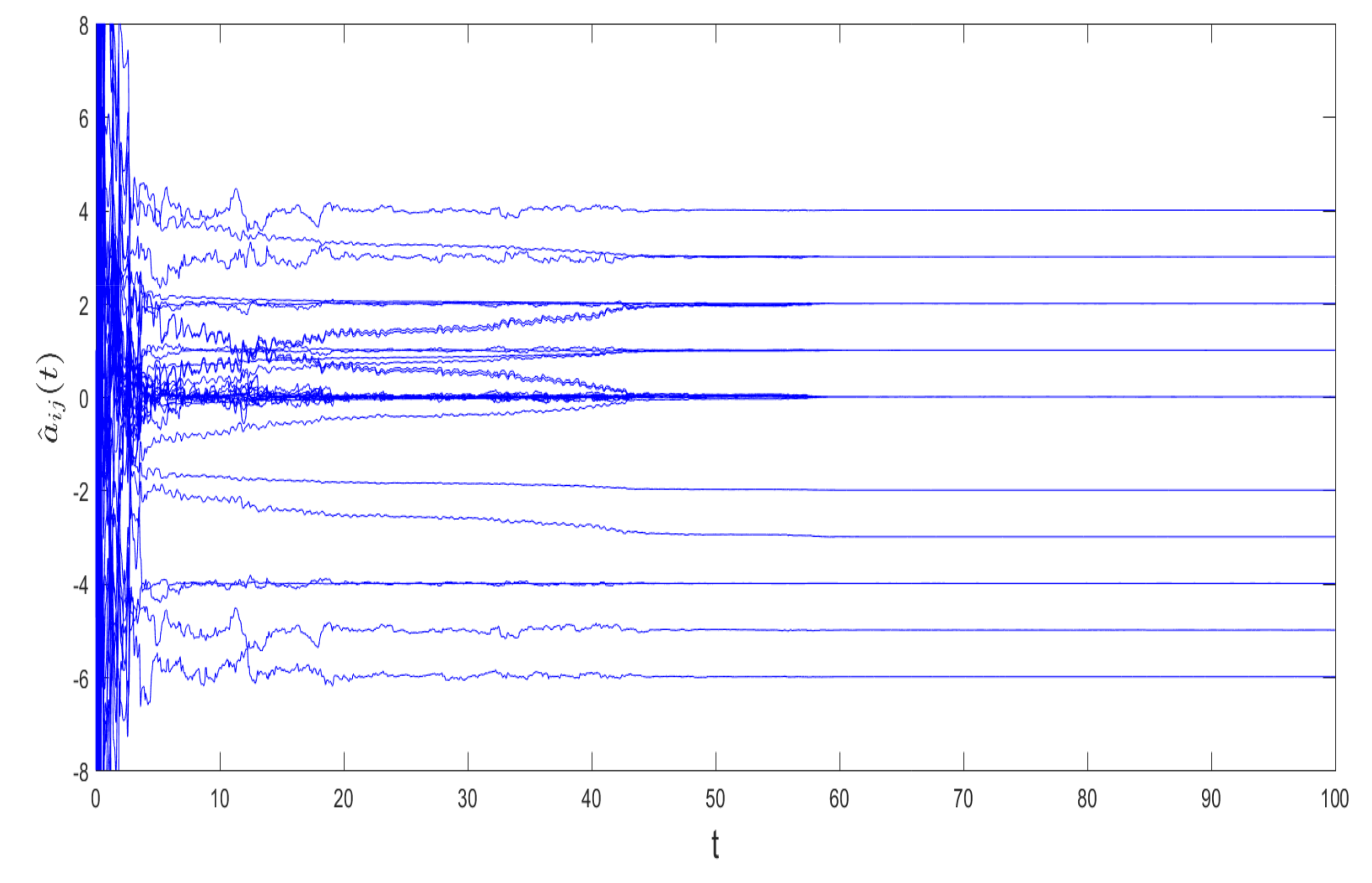
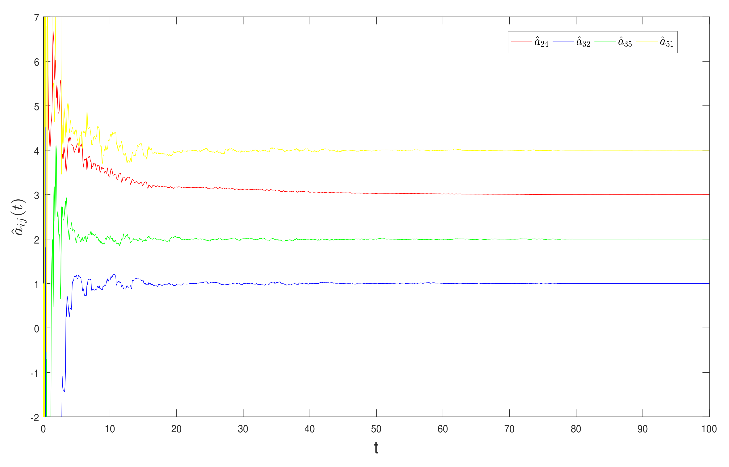
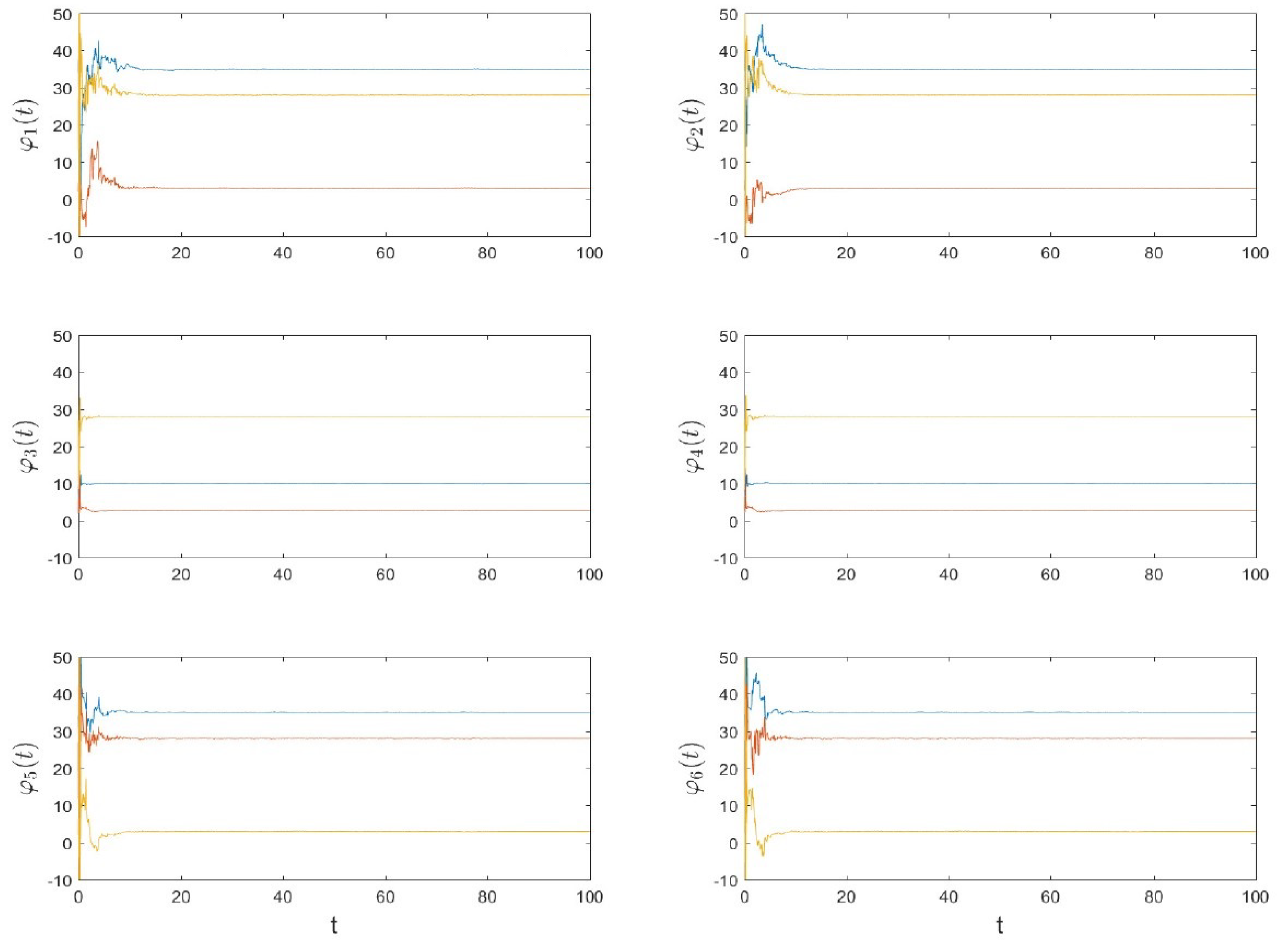
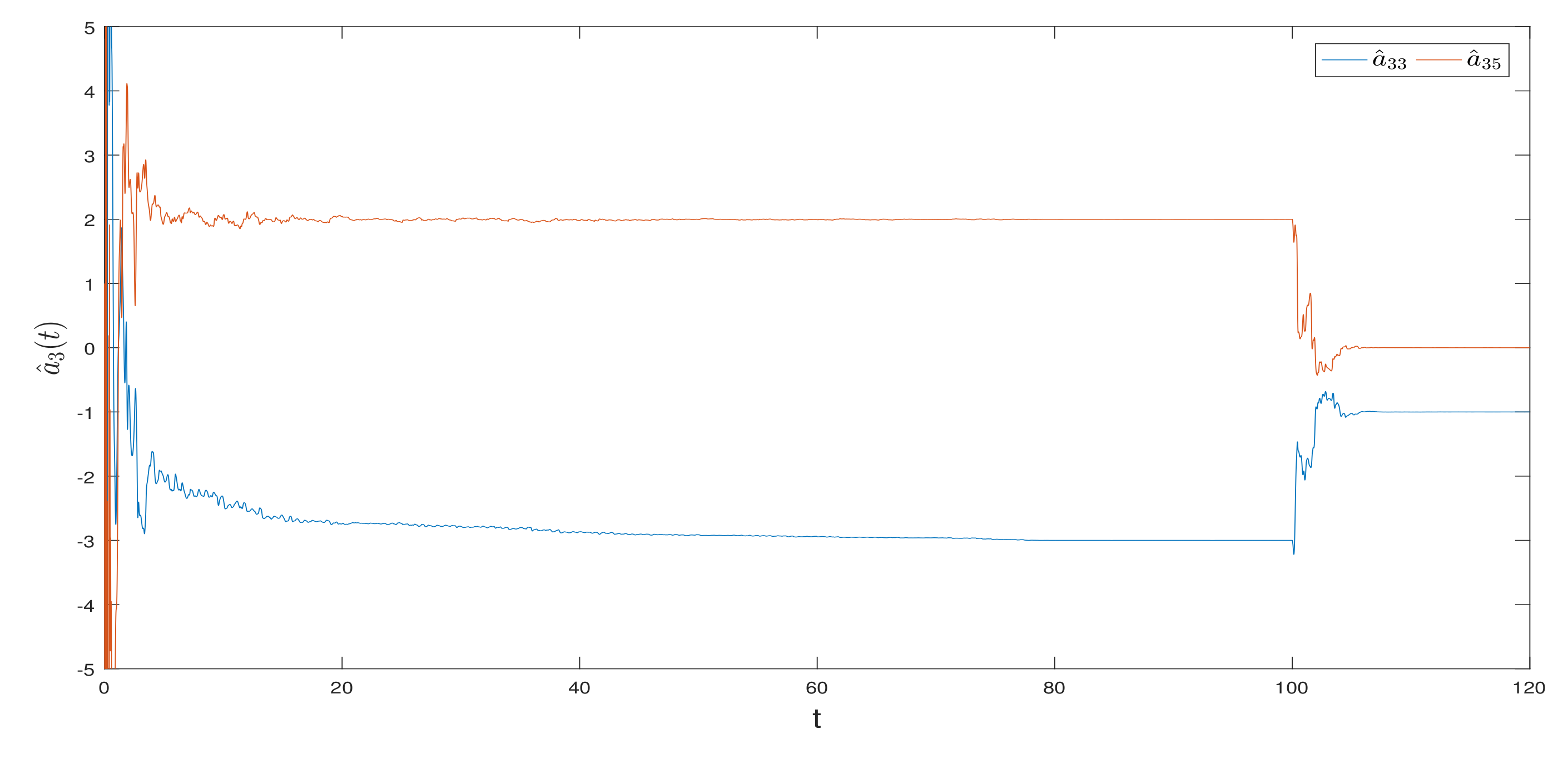
4. Numerical Examples

Consider a fractional-order dynamical network with six nodes, and choose the node dynamics as the fractional-order Chen system [33]

$$\begin{array}{ccc}\hfill & D^{{\alpha }_i}{x}_i=\left\{\begin{array}{c}{\varphi }_{i1}(x_{i2}-x_{i1}),\hfill \\ ({\varphi }_{i3}-{\varphi }_{i1})x_{i1}-x_{i1}{x}_{i3}+{\varphi }_{i3}{x}_{i2},\hfill \\ x_{i1}{x}_{i2}-{\varphi }_{i2}{x}_{i3}.\hfill \end{array}\right.\hfill & \hfill i=1,2,\end{array}$$

and the fractional-order Lorenz system [34]

$$\begin{array}{ccc}\hfill & D^{{\alpha }_i}{x}_i=\left\{\begin{array}{c}{\varphi }_{i1}(x_{i2}-x_{i1}),\hfill \\ {\varphi }_{i3}{x}_{i1}-x_{i1}{x}_{i3}-x_{i2},\hfill \\ x_{i1}{x}_{i2}-{\varphi }_{i2}{x}_{i3}.\hfill \end{array}\right.\hfill & \hfill i=3,4,\end{array}$$

and the fractional-order Lü system [35]

$$\begin{array}{ccc}\hfill & D^{{\alpha }_i}{x}_i=\left\{\begin{array}{c}{\varphi }_{i1}(x_{i2}-x_{i1}),\hfill \\ -x_{i1}{x}_{i3}+{\varphi }_{i2}{x}_{i2},\hfill \\ x_{i1}{x}_{i2}-{\varphi }_{i3}{x}_{i3}.\hfill \end{array}\right.\hfill & \hfill i=5,6,\end{array}$$

where $({\alpha }_1,{\alpha }_2,\cdots ,{\alpha }_6)=(0.97,0.98,0.995,0.998,0.99,0.99)$, ${\varphi }_1={\varphi }_2={(35,3,28)}^T$, ${\varphi }_3={\varphi }_4={(10,8/3,28)}^T$ and ${\varphi }_5={\varphi }_6={(35,28,3)}^T$.

Choose $c=0.1$, $H=diag(1,1,1)$ and

$$A=\left[\begin{array}{cccccc}-5& 3& 2& 0& 0& 0\\ 0& -4& 1& 3& 0& 0\\ 0& 1& -3& 0& 2& 0\\ 0& 1& 1& -2& 0& 0\\ 4& 0& 2& 0& -6& 0\\ 0& 2& 0& 2& 0& -4\end{array}\right].$$

Firstly, assume that only A is unknown. Choose the adaptive gains $\theta =1.6,{\mu }_{ij}=16$, the initial values $w\left(0\right)=0.1,{\widehat{a}}_{ij}\left(0\right)=1,$ for $i,j=1,2,\cdots ,6$, the initial values of the state variable $y_i\left(0\right)={(1+0.2i,2+0.2i,3+0.2i)}^T$ and ${\widehat{y}}_i\left(0\right)={(6+0.2i,5+0.2i,4+0.2i)}^T$. Figure 1 shows the evolution of ${\widehat{a}}_{ij}\left(t\right)$. For a clearer view, Figure 2 shows the orbits of ${\widehat{a}}_{24}\left(t\right)$, ${\widehat{a}}_{32}\left(t\right)$, ${\widehat{a}}_{35}\left(t\right)$ and ${\widehat{a}}_{51}\left(t\right)$. Clearly, the unknown topology is effectively identified at about $t=50$.

Secondly, assume that both A and ${\varphi }_i$ are unknown. Choose $\theta =1.6,{\mu }_{ij}=16,{\xi }_{ij}=25$, $w\left(0\right)=0.1,{\widehat{a}}_{ij}\left(0\right)=1$, ${\phi }_1\left(0\right)={(34,2,27)}^T$, ${\phi }_2\left(0\right)={(34.5,2.5,27.5)}^T$, ${\phi }_3\left(0\right)={(9,2,27)}^T$, ${\phi }_4\left(0\right)={(9.5,2.5,27.5)}^T$, ${\phi }_5\left(0\right)={(34,27,2)}^T$, ${\phi }_6\left(0\right)={(34.5,27.5,2.5)}^T,$ for $i,j=1,2,\cdots ,6$, $y_i\left(0\right)={(1+0.2i,2+0.2i,3+0.2i)}^T$ and ${\widehat{y}}_i\left(0\right)={(6+0.2i,5+0.2i,4+0.2i)}^T$. Figure 3 and Figure 4 show some orbits of ${\widehat{a}}_{ij}\left(t\right)$ and $\phi \left(t\right)$, respectively. Compared with Example 1, the topology identification needs more times. That is, the unknown system parameters have a great influence on the topology identification. How to improve the performance deserve further studies.

Finally, suppose that $a_{35}=2$ switches to $a_{35}=0$ at $t=100$ in the first example. Figure 5 shows that $a_{35}$ is identified quickly. That is, the network estimator (4) has good performance in real-time monitoring. From the practical viewpoint, the designed estimator can be used to monitor the switching phenomenon in circuits.

5. Conclusions and Discussions

The structure identification problem of uncertain fractional-order complex networks with different orders is investigated. Two network estimators are designed via adaptive feedback control and parameter updating laws. The valuable results for the integer-order networks and the fractional-order networks with the same order are generalized to the networks with different fractional orders. In this paper, all the state variables are assumed to be observable. In real cases, the state variables may be partially observable [11]. Thus, how to identify the topology from partial observations for fractional-order networks, especially with different orders, deserves further studies. On the other hand, many other methods are introduced to address the issue of integer-order systems. Compressive sensing based on transient dynamics is used to identify the topology for power systems [9]. An MILP method is used for distributed systems [10]. We will adopt the mentioned methods to consider the issue of fractional-order networks in future studies.

References

1. Su, H.; Chen, D.; Pan, G.J.; Zeng, Z. Identification of Network Topology Variations Based on Spectral Entropy. IEEE Trans. Cybern. 2021. [Google Scholar] [CrossRef]
2. Zhu, S.; Zhou, J.; Lu, J.A. Identifying partial topology of complex dynamical networks via a pinning mechanism. Chaos 2018, 28. [Google Scholar] [CrossRef]
3. Li, G.; Li, N.; Liu, S.; Wu, X. Compressive sensing-based topology identification of multilayer networks. Chaos 2019, 29. [Google Scholar] [CrossRef]
4. Van Waarde, H.J.; Tesi, P.; Camlibel, M.K. Topology reconstruction of dynamical networks via constrained lyapunov equations. IEEE Trans. Autom. Control 2019, 64, 4300–4306. [Google Scholar] [CrossRef] [Green Version]
5. Wang, X.; Gu, H.; Chen, Y.; Lü, J. Recovering node parameters and topologies of uncertain non-linearly coupled complex networks. IET Control Theory Appl. 2020, 14, 105–115. [Google Scholar] [CrossRef]
6. Wang, Y.; Wu, X.; Lu, J.; Lu, J.A.; Dsouza, R.M. Topology Identification in Two-Layer Complex Dynamical Networks. IEEE Trans. Netw. Sci. Eng. 2020, 7, 538–548. [Google Scholar] [CrossRef]
7. Zhu, S.; Zhou, J.; Chen, G.; Lu, J.A. A New Method for Topology Identification of Complex Dynamical Networks. IEEE Trans. Cybern. 2021, 51, 2224–2231. [Google Scholar] [CrossRef]
8. Yao, X.; Xia, D.; Zhang, C. Topology identification of multi-weighted complex networks based on adaptive synchronization: A graph-theoretic approach. Math. Methods Appl. Sci. 2021, 44, 1570–1584. [Google Scholar] [CrossRef]
9. Ding, L.; Li, W.; Nie, S.; Hu, P. Topology Identification for Power Systems via Compressive Sensing Based on Transient Dynamics. IEEE Trans. Circuits Syst. II Express Briefs 2020, 67, 3202–3206. [Google Scholar] [CrossRef]
10. Farajollahi, M.; Shahsavari, A.; Mohsenian-Rad, H. Topology Identification in Distribution Systems Using Line Current Sensors: An MILP Approach. IEEE Trans. Smart Grid 2020, 11, 1159–1170. [Google Scholar] [CrossRef]
11. Coutino, M.; Isufi, E.; Maehara, T.; Leus, G. State-Space Network Topology Identification from Partial Observations. IEEE Trans. Signal Inf. Process. Over Netw. 2020, 6, 211–225. [Google Scholar] [CrossRef] [Green Version]
12. Zhang, J.; Wang, Y.; Weng, Y.; Zhang, N. Topology Identification and Line Parameter Estimation for Non-PMU Distribution Network: A Numerical Method. IEEE Trans. Smart Grid 2020, 11, 4440–4453. [Google Scholar] [CrossRef]
13. Liu, H.; Li, Y.; Li, Z.; Lu, J.; Lu, J.A. Topology Identification of Multilink Complex Dynamical Networks via Adaptive Observers Incorporating Chaotic Exosignals. IEEE Trans. Cybern. 2021. [Google Scholar] [CrossRef]
14. He, X.; Qiu, R.C.; Ai, Q.; Zhu, T. A Hybrid Framework for Topology Identification of Distribution Grid with Renewables Integration. IEEE Trans. Power Syst. 2021, 36, 1493–1503. [Google Scholar] [CrossRef]
15. van Waarde, H.J.; Tesi, P.; Camlibel, M.K. Topology identification of heterogeneous networks: Identifiability and reconstruction. Automatica 2021, 123, 109331. [Google Scholar] [CrossRef]
16. Podlubny, I. Fractional Differential Equations: An Introduction to Fractional Derivatives, Fractional Differential Equations, to Methods of Their Solution (Mathematics in Science and Engineering); Academic Press: Cambridge, MA, SUA, 1999; Volume 198. [Google Scholar]
17. Kilbas, A.; Srivastava, H.; Trujillo, J. Theory and Application of Fractional Differential Equations; Elsevier: New York, NY, USA, 1964; Volume 1, p. 1489. [Google Scholar]
18. Si, G.; Sun, Z.; Zhang, H.; Zhang, Y. Parameter estimation and topology identification of uncertain fractional order complex networks. Commun. Nonlinear Sci. Numer. Simul. 2012, 17, 5158–5171. [Google Scholar] [CrossRef]
19. Du, L.; Yang, Y.; Lei, Y. Synchronization in a fractional-order dynamic network with uncertain parameters using an adaptive control strategy. Appl. Math. Mech. (Engl. Ed.) 2018, 39, 353–364. [Google Scholar] [CrossRef]
20. Li, H.L.; Cao, J.; Jiang, H.; Alsaedi, A. Finite-time synchronization and parameter identification of uncertain fractional-order complex networks. Phys. A Stat. Mech. Its Appl. 2019, 533. [Google Scholar] [CrossRef]
21. Du, H. Modified function projective synchronization between two fractional-order complex dynamical networks with unknown parameters and unknown bounded external disturbances. Phys. A Stat. Mech. Its Appl. 2019, 526. [Google Scholar] [CrossRef]
22. Jia, Y.; Wu, H. Global synchronization in finite time for fractional-order coupling complex dynamical networks with discontinuous dynamic nodes. Neurocomputing 2019, 358, 20–32. [Google Scholar] [CrossRef]
23. Xu, Y.; Li, Y.; Li, W.; Feng, J. Synchronization of multi-links impulsive fractional-order complex networks via feedback control based on discrete-time state observations. Neurocomputing 2020, 406, 224–233. [Google Scholar] [CrossRef]
24. Yang, Q.; Wu, H.; Cao, J. Pinning exponential cluster synchronization for fractional-order complex dynamical networks with switching topology and mode-dependent impulses. Neurocomputing 2021, 428, 182–194. [Google Scholar] [CrossRef]
25. Zheng, Y.; Wu, X.; He, G.; Wang, W. Topology identification of fractional-order complex dynamical networks based on auxiliary-system approach. Chaos 2021, 31. [Google Scholar] [CrossRef] [PubMed]
26. Xiao, J.; Cao, J.; Cheng, J.; Zhong, S.; Wen, S. Novel methods to finite-time Mittag-Leffler synchronization problem of fractional-order quaternion-valued neural networks. Inf. Sci. 2020, 526, 221–244. [Google Scholar] [CrossRef]
27. Cheng, Y.; Hu, T.; Li, Y.; Zhang, X.; Zhong, S. Delay-dependent consensus criteria for fractional-order Takagi-Sugeno fuzzy multi-agent systems with time delay. Inf. Sci. 2021, 560, 456–475. [Google Scholar] [CrossRef]
28. Hu, T.; He, Z.; Zhang, X.; Zhong, S. Event-triggered consensus strategy for uncertain topological fractional-order multiagent systems based on Takagi–Sugeno fuzzy models. Inf. Sci. 2021, 551, 304–323. [Google Scholar] [CrossRef]
29. Kaczorek, T. Positive linear systems consisting of n subsystems with different fractional orders. IEEE Trans. Circuits Syst. I Regul. Pap. 2011, 58, 1203–1210. [Google Scholar] [CrossRef]
30. Datsko, B.Y.; Gafiychuk, V.V. Mathematical modeling of fractional reaction-diffusion systems with different order time derivatives. J. Math. Sci. 2010, 165, 392–402. [Google Scholar] [CrossRef]
31. Li, C.; Deng, W. Remarks on fractional derivatives. Appl. Math. Comput. 2007, 187, 777–784. [Google Scholar] [CrossRef]
32. Aguila-Camacho, N.; Duarte-Mermoud, M.A.; Gallegos, J.A. Lyapunov functions for fractional order systems. Commun. Nonlinear Sci. Numer. Simul. 2014, 19, 2951–2957. [Google Scholar] [CrossRef]
33. Li, C.; Chen, G. Chaos in the fractional order Chen system and its control. Chaos Solitons Fractals 2004, 22, 549–554. [Google Scholar] [CrossRef]
34. Grigorenko, I.; Grigorenko, E. Chaotic Dynamics of the Fractional Lorenz System. Phys. Rev. Lett. 2003, 91. [Google Scholar] [CrossRef] [PubMed]
35. Lu, J.G. Chaotic dynamics of the fractional-order Lü system and its synchronization. Phys. Lett. Sect. A Gen. At. Solid State Phys. 2006, 354, 305–311. [Google Scholar] [CrossRef]
Figure 1. The evolution of a ^ i j ( t ) , i , j = 1 , 2 , , 6 .
Mathematics 09 02096 g001
Figure 2. (Color online) The orbits of a ^ 24 ( t ) , a ^ 32 ( t ) , a ^ 35 ( t ) and a ^ 51 ( t ) .
Mathematics 09 02096 g002
Figure 3. (Color online) The orbits of a ^ 24 ( t ) , a ^ 32 ( t ) , a ^ 35 ( t ) and a ^ 51 ( t ) .
Mathematics 09 02096 g003
Figure 4. (Color online) The blue, red and yellow lines denote the first, second and third components of the state variables φ i ( t ) respectively.
Mathematics 09 02096 g004
Figure 5. (Color online) Identification of the switching topology.
Mathematics 09 02096 g005
Publisher’s Note: MDPI stays neutral with regard to jurisdictional claims in published maps and institutional affiliations.