Abstract
The perishable milk products industry has to deal with multiple pressures such as demand forecasting, price fluctuations, lead time, order batching, and inflated orders along with difficulties of climatic and traffic conditions, storage areas and shipment in unfavorable circumstances. The Indian dairy industry faces immense wattage issue due to improper infrastructure for the cold chain storage facilities, resulting in unsatisfied customers. A study is undertaken to comprehend the supply chain framework that handles perishability issues in production and distribution. Researchers propose a multi-objective mixed-integer non-linear supply chain coordination model under uncertain environments to minimize the cost of transportation, offset wastage of products and neutralize the losses due to insufficiencies of transit and storage amenities. The proposed model is meant for managing the delivery with lesser deterioration losses for producers, warehouses, and retailers. The model considers various costs for holding, halting, discounts on purchased cost, transportation cost for truckload policy under regular and unforeseen circumstances of curfew, and identify the rate of deterioration to know the impact on the cost for all players involved in the SCM framework. To handle uncertainty of objective functions, fuzzy set concepts and the defuzzification method are imposed, and fuzzy non-linear programming algorithms are used to get the single objective function from the defuzzified multi-objective functions. Data analysis is done on Lingo 18.0 software. Rate of deterioration is highest for the warehouse, which indicates that efforts should be made to augment warehouse facilities for less spoilage to reduce losses in cost. Finally, the study ends with main findings, conclusions, limitations and future scopes.
1. Introduction
The challenges posed by deterioration are not new for the supply chain of perishable products, as this phenomenon is a common and ordinary one and accounts for significant losses in terms of cost. Deterioration in the general term refers to a process of decay, damage, expiry, and devaluation of a product with time []. Deterioration is a realistic and physical phenomenon, so the formulation of an appropriate strategy for managing the perishability of deteriorating items is established and expected fact. The management of perishable products requires an efficient supply chain coupled with a comprehensive warehouse with a temperature-controlled facility and an uninterrupted cold chain system throughout to keep the rate of deterioration and cost under control. Supply chains for perishable products are complex owing to the perishable nature of the products, as the value of the product goes down with temperature and humidity []. Owing to increasing demand for a variety of multi-flavored products such as head induced, light-induced, oxidized and transmitted flavored products, warehouses need to accommodate more inventories and do so with the latest equipment. Lack of proper infrastructure and inefficient supply chain could easily accentuate the wastage []; consequently, considerable attention should be paid to find economically viable solutions to develop efficient cold supply chains to reduce wastage. The areas of concern are not limited to supply chain only, as the perishable milk products industry has to endure multiple challenges of product’s spoilage or decay due to its perishable nature [], short lifetime. and uncertain demand [,]. In addition to this, another research study focuses on various parameters such as uncertain prices, batch order along with inflated order, and lead time to satisfy immediate demands []. Some other issues requiring contemplation are the climatic conditions, state of storage facilities, traffic congestion and unforeseen delivery schedules []. The resultant outcome of all these problems is a considerable amount of losses in terms of the product itself, and related cost of transportation, storage, and transit inefficacies []. Not to be forgotten is that these supply chains also call for flexibility in the terms of response capacity related to volume and variety due to changing customer’s preferences [,] and improvement in supply chain resilience against transportation disruptions. Additionally, these supply chains have to manage efficiently to avoid management errors, environmental changes, and economic imbalances []. Technological advancements have made things a bit easier for these supply chains by providing facilities with tracing and tracking to keep a check on inventory levels and product quality leading to improved performance and less spoilage []. By integrating, organizing, and sharing information and introducing strong institutional and policy frameworks perishable supply chain industry can boost its endurance level and make headways in economic prospects [].
The point of discussion is if this process is seemingly so simple, then why are organizations incurring recurring losses due to deterioration in their supply of perishable products? Here we would like to argue that though modern technologies and information-sharing systems have bought integration into transportation and warehouse management by connecting vehicles, warehouses, and other allied facilities under one network lack of awareness about functional technicalities and ground-level understanding is found to be missing in many places. For example, the longevity of perishable products is not only accomplished by temperature control but also by proper handling of control techniques and mechanisms. The selection of appropriate temperature for the preservation of perishable products is essentially the main factor as this is the most important environmental factor that influences the deterioration rate of perishable products. However, the fact cannot be ignored that multiple elements of the supply chain of perishable products like uncertain demand; technical issues, disruptions of the production process [], price of the product, the life cycle of the product [], inventory types and cost, types of sellers and buyers, lot size, holding and halting cost, inspection cost, safety stocks, discounted cost, shelf life, and transportation cost must be interplayed and managed effectively for optimal results.
This research is based on real-time data provided by a leading dairy product chain in India. Our focus of the study is the deterioration rate of four dairy products and their related cost implications for the supply chain player by working on the complexities of deterioration, transport, uncertainty in demand, fluctuating price, and transit inefficiencies. The study takes into account the deterioration rate, discounted costs at different stages based on quantity, flexibility in transportation cost for unforeseen situations, holding, halting, and inspection cost impacts at three different stages based on supplier, warehouse, and retailer. The objectives of the study are to identify various levels of deterioration and a proposition to eliminate the risk of higher cost gradients. The study addresses the issues of of multi-product supply chain complexity in three echelon scenarios, multi-location, uncertain demand for maximum product, and a certain demand for few products and certain period with the possibility of uncertainty in holding cost for given situations. The key difference in our study is that it has multiple items and three periods, and it has taken route disruptions due to uncertain circumstances in its loop. Most of the past studies are focused on single-item supply chain complexity; however, our study is of great interest to researchers as it is based on real-time data to let us explore the interplay between multi-item supply chain complexities. To provide a sound foundation to our work, we have based it on the studies conducted by numerous researchers on multiple issues related to perishable supply chains based on quality deterioration.
This paper continues with a review of the literature in Section 2 to understand the major work done in the field of management of the perishability of the supply chain. This section reviews the literature regarding various parameters of the perishable supply chain and various approaches of converting a multi-objective function to a single-objective function to identify the research gaps. Detailed information about the dairy industry in the Indian scenario and collection of data is given in Section 3, and discussions are in Section 4, which describes the analysis of data. A three-echelon multiobjective mixed-integer fuzzy nonlinear programming model (MOMIFNLP) is proposed to find a solution to the given problem of the organization in Section 4.2.
2. Literature Review
Environmental uncertainties are natural to the functioning of supply chains, so most organizations design their supply chain loops to match uncertainty. However, this uncertainty can be overcome to some extent by including flexibility and resilience in the supply chain without compromising their operational efficiency and effectiveness []. In a realistic scenario, this flexibility changes according to the demand of the products, changing preferences of the customers, and regulations impacting cost; hence, while designing a model, all these factors of uncertainty and flexibility must be included in the framework. Many instrument models have been developed to measure flexibility [,,], and eventually, multiple models based on the dimensions of the flexibility [,], connecting flexibility to the supply chain [], have also been proposed. Exploration has also been done to establish the relationship between flexibility and supply chain drivers to prioritize dimensions for improvement []. Some researchers, however, have argued that supply chain flexibilities are costly [] or not economically viable [,]; subsequently, a careful approach is required before introducing flexibility into the supply chain infrastructure.
An understanding of the nature of perishable versus non-perishable, deterioration rate, and the uncertainty of the product, as well as complexities related to production, supply, and mode of distribution of the product, could provide the required resilience to the organizations to design customized supply chains. For example, the inventory management mode of the transport time frame for a perishable and deteriorating product is different from that of a non-perishable one. In addition, there is a difference in the inventory management of two types of products, the first with a fixed lifetime, and second, which undergo rapid decay []. Both types of products require different strategies and customized supply chain that could meet the required specifications. The credit of introducing the concept of deterioration could be given to the seminal work of Ghare [], who proposed optimal ordering policies by developing an EOQ model for an item with exponential decay and constant demand. In other seminal literature, the concept of deterioration can be attributed to Van Zyl [], who worked on a model with two shelf lives for perishable goods as stated by Nahmias [] in a review of the early literature on ordering policies. A close look at the research studies brings out various dimensions in which the study of deterioration has been carried out: lot size and continuous-time []; Weibull distribution deterioration []; the variable rate of deterioration with a finite rate of production []; deteriorating inventory with a linear trend in demand []; and an inventory model with uncertain demand and deterioration rate implemented []. Many researchers have chosen a fuzzy environment in inventory problems to handle uncertain information of demand and deterioration rate of the products; however, in the case of dairy products, no specific research has been done.
Researchers have also experimented with a variety of models for managing deteriorating inventory in the context of price fluctuations, demand, storage, shortages, shelf life issues, lot sizing, location, warehouses, transport, etc. Hsu [] focused on the stock’s shelf life for perishable products to mange the stock’s deterioriation rate and holding cost for the economic lot size model. Pervin et al. [] analyzed an inventory model for deteriorating items where deterioration rate was followed by a stochastic environment such as Weibull distribution. Furthermore, Pervin et al. [] proposed another inventory model based on deterioration rate for stock and price-dependent demands with preservation investment amount. Lütke Entrup et al. [] proposed varied shelf life values for a yogurt production plant having issues for the production planing based on mixed integer linear programming. Mishra [] analyzed a dynamic medium-term production planning and scheduling problem of a large German brewery, which is characterized by sequence-dependent setup times and costs, capacity restrictions for the filling machine and the inventory, and carrying over the setup state. Hou and Lin [] proposed a model for deteriorating inventory and a consumption rate dependent on stock and shortages dependent on inflation and time discounting.
The traditional lot size model of inventory is extended to accommodate changes in demand along with an increase in cost []. Experimentation with the lot size of inventory for perishable goods has been done by including expiration dates and advance payments []. The model for deteriorating inventory based on inventory management modes and inventory demand is proposed by Bakker et al. [], and the model for a perishable items with deteriorating inventory with pricing problems is proposed by Chowdhury et al. [] and Chang et al. []. Keeping an element of perishability, price change, and decrease in demand, a two-echelon supply chain model is presented by Wang and Lin [] to develop an optimal replenishment policy. Furthermore, the inventory model with two-period pricing problems has been proposed by Herbon [], Dye and Hsieh []. Management of lot sizes, replenishment cycle, and schedules in particular for products with short life and financial volatility has been explored by doing a sensitivity analysis of the proposed optimization model by Ali et al. []. Another inventory model that includes approximate deterioration free time and credibility limitations for products with a longer deterioration rate is proposed by Soni []. An EOQ model inclusive of the effect of inflation, volume agility, and variable demand rate is presented by Tayal et al. []. Another model for perishable inventory, decentralize supply chain and pricing problems has been given by Chung et al. []. In another research study comprising variants of the capacitated lot-sizing problems, stochastic programming models, and explicit uncertainty modeling, inventory models are given by Raiconi et al. [], in which a variant of the capacitated lot-sizing problem accounts for lifetime constraints, such as perishable items with known shelf-lives in accordance with the regulatory framework. The dynamic programming method is applied to the inventory system for perishable products to study the effect of inspection polices [].
Inventory management is also dependent on the lifetime constraints of products [], deterioration in production [], and deterioration in supply chain planning [], which has a direct relation with the demand of the product. Chen and Chen [] proposed a model focusing on two factors—price-dependent demand and a lifetime-dependent deterioration rate—to calculate periodic prices and economical lot sizing for maximum profit, since the price of the product is directly linked to the demand, which plays an important role in inventory management, especially in the case of perishable products. As identified by Amorim et al. [], perishable product consumers confirm the expiry dates for freshness accordingly, so that customer’s preferences can easily bring about variations in the demand of a product [], for example, flavored dairy products; demand for chilled dairy products is high in the summer season based on climatic conditions. The volatility in demand eventually creates uncertainty, leading to companies creating more inventory buffers to cope with demand fluctuations. Demand is generally categorized into deterministic and stochastic categories []. Studies have been conducted on various aspects of demand such as time-independence, in which lifespan and utility of the product is pre-specified []; time proportional []; time-varying demand [], maximizing profit [,]; expiration date []; stock-dependent demand [,,]; quality-dependent demand [,]; credit-period-dependent demand [,,,]; and age-dependent demand rate []. Pervin et al. [] studied a two-echelon inventory model by offering a trade-credit period in a year by the manufacturer to the retailer. Additionally, in that paper, demand for a manufacturer is time-dependent and that for a retailer is stock-dependent. Work has also been done on the demand rate dependency on the multivariate function of the selling price, expiration, and display of stocks []. Demand dependency on the displayed stock and difference between the current selling price and reference price [], current price, and historical price-dependent [], inflation []. Pervin et al. [] formulated an integrated vendor-buyer model including a quadratic demand rate for deteriorating items.
The complications of fluctuating demand coupled with the deterioration rate of the product and uncertainty in time-push organizations to bring alterations in their production processes, warehouse proportions, and location and modes of transportation. A two-stage fixed cost transportation capacity production model has been proposed by Kaminsky and Simchi-Levi []. Hwang [] examined a case-based stochastic set location problem for managing deteriorating and ameliorating items to be adjusted in minimal storage facilities. The model presented by Yang [] was based on a loop cycle from start and end. A push–pull production distribution two-stage supply chain has been mentioned in the work of Ahn and Kaminsky []. Deterioration and lifetime constraint models are also analyzed under the specification of multiple-warehouse models by Hwang [], Yang [] and Pal et al. []. Pal et al. [] applied MILNP ( mixed integer non-linear programming) model for a two-warehouse inventory based on a genetic algorithm with the objective of optimal number of replenishment and lot size a two-warehouse inventory system for deteriorating items. Rieksts and Ventura [] proposed a model based on two transportation freight types of mode to have an optimal inventory system for a warehouse and a retailer. Hwang et al. [] took into consideration the quantity discounts based on purchasing cost and freight cost for finding optimal order quantity. Ertogral [] investigated a single-stage multi-item un-capacitated dynamic lot-sizing problem (MILSP) with transportation costs and dynamic demand. Mendoza and Ventura [] proposed an economic order quantity model for discount based on all and incremental quantity having full truckload and less than truckload carriers. Tersine and Barman [], and Gandhi et al. [] incorporated quantity and freight discounts into the lot size decision in a deterministic economic order quantity system.
In recent studies, Behzadi et al. [] proposed eliminating the risk in perishable agribusiness product supply chains by employing policies for infrequent and frequent harvest seasons and yield instabilities integrating exponential function for perishable product to propose two stage stochastic model []. Lot sizing of perishable products that get affected by inventory losses and uncertainty in the product demand has been explored by Coniglio et al. [], in which they proposed a hybrid robust-stochastic approach to determine optimal procurement policies and transfer plan for perishable products. Pahl and Voß [] put a focus on waiting times due to suboptimal planning, depreciation of parts and products while waiting, and, thus, deteriorated quality of items or even unusable products.
It can be added here that the major work in supply chain management for perishable products is focused around inventory management and single items, lot-sizing problems, two periods, and two warehouses. We would like to consider the work done by Pahl and Voß []. Brahimi et al. [], who have explored the research studies published in between 2004 until 2016 for problems of single item lot size for searching methods of exact and heuristic solution. They make a classification of research according to constraints on resources, integrating decisions on supply chain management.
The organization under study has been facing the problem of inventory losses, along with higher costs, and the focus of the study is caentered around the supply chain complexity of dairy-related multi-items in a three-period scenario where the demand is certain for one product and uncertain for the other three products and managing the delivery of milk in the morning and evening shifts daily, by keeping an element of uncertain demand and transport disruption due to unexpected route changes due to curfew, road blockages, etc. We have proposed a model for the deterioration of dairy products in the form of a multiobjective mixed-integer nonlinear optimization problem using real-world data from Indian firms. A brief overview of the Indian milk industry is given in the next section, which is followed by our method of data collection comprising target selected organizations, area of research, time frame statements, and assumptions of the model.
3. Data Collection
3.1. Indian Dairy Sector Scenario
Indian dairy industry is symbolic of its socio-economic growth, which has managed to utilize the national resources to build a milk production industry that boasts of strong rural milk procurement infrastructure, improved cattle productivity, and a network of more than a million milk vendors and a billion consumers. The milk production in India has seen steady growth for many decades, and hence India has managed to become the largest producer of milk in the world (http://www.indianmirror.com/indian-industries/dairy.html accessed on 20 January 2020 at 7.25 p.m.). With 70 million households engaged in dairy farming, milk production in the year 2016–2017 has risen by 6% and has reached the mark of 18.81% and per capital availability of milk stands at 351 gm/day (http://www.india.com/business/milk-production-in-india-up-by-18-81-in-2016-17-dairy-farmers-income-hike accessed on 12 June 2019 at 6.12 a.m.). Besides offering greater market access to farmers, it also provides profitable business opportunities to multiple players in rural and urban areas with the income of dairy farmers increasing 23.77% in 2014–2017 (http://www.livemint.com/Industry/qmoDKWWG9EOBFdwnZcTNiM/Milk-output-rises-19-dairy-farmers-incom accessed on 2 April 2019 at 7.54 a.m.). Dairy cooperatives and contractors of private dairies and large-scale dairy farmers account for the organized sector of the dairy industry and have a major share of processed milk and associated value-adding products like cheese, butter, curd, buttermilk, yogurt, and probiotic drinks. These cooperatives have organized the procurement network of milk from local farmers and have distribution channels for efficient distribution of its supplies, taking the dairy industry market to reach a level of 16,368 billion in 2022 with an expected CAGR of 16% during 2017–2022 (https://www.imarcgroup.com/dairy-industry-in-india accessed on 12 March 2019 at 4.23 p.m.). However, the Indian dairy industry does have other players in the form of an unorganized sector comprising local milkmen and small-scale farmers. The supply chain of the milk sector in India (Figure 1) is run by both organized and unorganized sectors, each managing their logistics in their own unique manner.
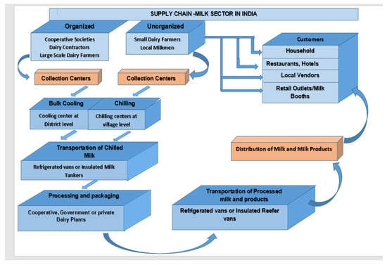
Figure 1.
Supply chain network of milk sector in India.
The logistics of milk in India is managed by multiple players in multiple stages. It sometimes becomes difficult because of a variety of challenges in procurement, distribution of the quality of milk, and many other related problems. The perishability of milk and milk products calls for a considerable amount of attention, and hence the present study focuses on the supply chain challenges of a popular milk cooperative of India for managing optimal quantity, leading to less deterioration at various stages in the supply chain. The name of the organization is held anonymous as requested by the organization.
3.2. Sample Organization Selection
The current study evaluates the supply chain network of leading organizations of India engaged in perishable milk-based products with a special focus on the network in the national capital, New Delhi, and its adjoining areas. The chosen organization is one of India’s leading milk product-based organizations and has more than four decades of operational experience of customer contentment delivery. The secret to staying ahead in the competition is to streamline its supply chain rights from demand forecasting for adequate inventory, modern inventory management practices, timely resupply orders, and quick delivery. Furthermore, by focusing on innovations in terms of product differentiation, to build flexible supply chains for uncertain times as in the current phase of lockdown, they have formulated proactive and collaborative planning processes, which can accommodate low response times to respond quickly to demand volatility and price fluctuations. Staying at par with the global counterparts, they have adopted a forward way of doing more with less, with shared service centers and payment counters and booths covering a wide range of geographical territories of India, with more than 50 sales offices, thousands of suppliers, and more than a million retailers. The strategy of these organizations is to connect the customer to the origin of the product. The procurement of products occurs through cooperative societies. These formal societies help in uniting the widely spread fragmented markets, and the payment is made to them at the time of delivery. These cooperative societies have collection centers where milk is deposited by farmers and is then further pooled and transferred to chilling and bulk milk cooling units, where it is cooled at a specified temperature. The next step is the transfer of milk to insulated tankers for transportation to processing plants to be tested and further processed and taken into milk tankers. Further utilization of milk into different categories of milk and milk products happens at processing centers, and from there, the products are dispatched to retail outlets and parlors.
3.3. Sample Area Selection
Data were collected from the centers of the given organization situated in New Delhi, one of the hottest regions of northern India. New Delhi is the capital city of India and the seat of the Indian government and house to corporate offices of many national and international organizations. Having the charm of incredible ancient monuments, an endless variety of cuisines, a variety of markets catering to the needs of heterogeneous customers, and the main international airport, which is a gateway to the rest of India, it remains host to a plethora of tourists and administrative and corporate travellers throughout the year. It also offers better job opportunities, a higher standard of living, better life style, and more exposure to learning, which makes it densely populated and prone to major traffic congestion during peak working hours. As it is the capital city, it hosts many nationally and internationally significant events that often cause traffic or road blockades due to VIP movements or lock downs.
3.4. Data Collection Time Frame
Since the weather reaches almost up to 48 C in the peak summer season, the possibility of deterioration is highest during this season. This season is more challenging and could bring better results for model testing; accordingly, data were collected for 21 days during the peak summer season in the first week of May, the second week of June, and the third week of July, with randomization of the data. The perishable products under consideration are Product I: Milk, Product II: Cheese, Product III: Curd, Product IV: Butter.
3.5. Statement of the Problem
The organization under consideration has been dealing with the problem of unsatisfied customers, high inventory holding cost, halting costs, and flexibility in transportation cost for the delivery of its perishable products in the capital city of New Delhi under foreseen conditions.
The supply chain model of the organization for the specified area has a framework shown in Figure 1.
Milk is procured at collection centers, and then milk and milk products are processed at processing centers. The two-stage supply chain model (Figure 2) integrates inventory and transportation modes, with three echelons: first, origin or source supplier; second, the intermediate node; and finally, the buyer/retailers as the final destination.
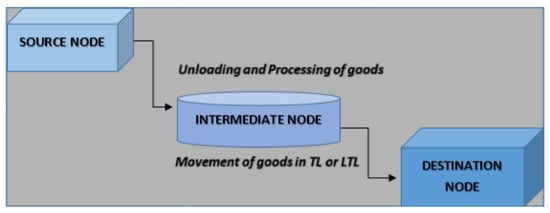
Figure 2.
Two-Stage supply chain model for three echelon.
The first stage involves the movement of goods from the source to the intermediate node (warehouse) where the unloading and further processing of goods for a specified period occurs.
The model includes quantity and freight discounts and has a fixed inspection cost; the holding cost is fixed until a particular time, and this cost then increases substantially.
The movement of goods from intermediate to the final destination is done in full truckloads (TL) or less than truckloads (LTL), which occurs in the second stage of the model.
3.6. Assumptions of the Model
The study aims to minimize the total cost of deterioration based on the procurement and distribution of these four products, namely P1: Milk; P2: Cheese; P3: Curd; P4: Butter, in the specified time frame of three weeks in the peak summer season. The study intends to include the issues of areas such as traffic congestion, roadblocks, and route change for uncertain situations like lockdown, curfew, political, or religious rallies into the delivery loop for finding an optimal solution to the given problem. The problem of uncertainty due to unexpected situations such as curfew or bandhs or rallies, as well as cultural or religious processions, has not been handled by previous researchers; consequently, this research gave us an opportunity to explore it.
The organization aims to manage the optimal order quantity with the minimum cost from the source to deal with the consumer’s daily demand based on the following:
- Cost of procurement;
- Inventory carrying cost;
- Transportation cost from source to the intermediate node;
- Holding cost at the intermediate node;
- Transportation cost from the intermediate node to the final destination;
- Inspection cost of the quantity received at the final destination;
- Inventory carrying cost at the final destination.
A reflect quantity and related purchase cost of each product are shown in Table A1, Table A2, Table A3, Table A4, Table A5, Table A6, Table A7, Table A8, Table A9, Table A10 and Table A11 in Appendix A. The price variation shown is indicative of different sellers offering the same product and includes the holding cost charged by different warehouses and retailers.
The data were collected during summer, so while transporting the weighted amount from the warehouse to retailers, truckload (TL) and less than truckload (LTL) policies may be used, where the capacity per truck is 250 kg. In the case of LTL policy, each extra unit of full truck capacity costs INR 6 (1 INR = 0.013 United States Dollars as of 12 April 2020). Ending inventory deterioration fraction is 1% at the destination.
3.7. Data Analysis
The data collected from the organization highlighted the specific problem areas aimed at finding an optimal solution to the problem. A multi-objective mixed-integer non-linear programming model under uncertainty is proposed. The model is meant to improve supply chain resilience to transportation disruptions, cost of transportation, holding and halting cost, and deterioration cost. We focused on a range of strategies for improving resilience, managing flexibility, minimizing redundancy, and establishing conducive trustworthy supply chain relations to have better agility.
4. Mathematical Model
The scenario presented in the study is a multi-period, multi-product, and supplier-warehouse two-stage supply chain framework that points towards finite horizon and finite time problems with uncertain daily demand. The current study intends to find solutions to the main problems: managing demand based on deterioration level and reduction of related total cost of inventory, procurement, transportation, halting, and holding to predict the deterioration rate for warehouses, retailer, and transported quantity from warehouse to retailer.
4.1. Model Proposition
A three-echelon supply chain model to optimize the cost related to inventory, distribution, and transportation-related activities would help in measuring goal attainment. Taking the EOQ model of transportation proposed by Gandhi et al. [], the problem stated in the current scenario calls for a two-stage system of finite planning horizon with uncertain demand and no shortages. It is expected that there is a certain amount of initial inventory of each product. The carrying cost does not depend on the unit price of purchase and transportation cost. The deterioration rate of inventory remains constant as a percentage of perished products in stored units, and the inspection cost is also assumed to be constant.
The model considers the uncertainty in the situation and proposes the transportation cost to be taken as 2000, 2200, and 2500 on the days when the route has to be changed due to lockdown, political voting, or religious functions or congestion instead of 1500, 1650, and 1700 depending on the availability from 3PL partners in the phase of these uncertainties.
The time considered under study is 21 days with the demand for milk in two shifts in a day for three days in particular. Morning delivery is done in TL and majority LTL is used for evening delivery. Please note that no discount is offered on LTL. The cost given by the organization is 131,000 in Indian rupees, and the target is to reduce this total cost.
4.2. Settings and Model Formulation
The proposed model consists of transportation modes with “three echelons”; first, the origin or source supplier, second, the warehouse as an intermediate node, and last, the retailer as the final destination. To formulate the proposed model, we consider sets and indices, parameters, decision variables, objective function, and constraints.
4.2.1. Sets and Indices
| p | period set |
| i | product set |
| l | product discount break point set |
Parameters:
| Purchased cost of the unit ith product at source supplier | |
| Holding cost of the unit ith product at the warehouse in the period p | |
| Holding cost of the ith product at the retailer in the period p | |
| Per unit weight of the ith product in kgs | |
| Transportation cost for each TL in the period p | |
| Morning demand for the ith product in the period p at the retailer | |
| Evening demand for the ith product in the period p at the retailer | |
| Morning consumption of ith product in the period p at the retailer | |
| Evening consumption of ith product in the period p at the retailer | |
| Cost per unit inspection of the products at the retailer | |
| M | Weight capacity per each full truck TL |
| Cost per kg of transporting in LTL mode | |
| Fractions of regular price supplier pays for the purchased ith product | |
| Fractions of regular price paying for transporting weigh | |
| Halting cost for the first day during transportation per S kg weight in the period p | |
| Halting cost per day for second day onward during transportation per S kg weight in the period p | |
| Quantity discount factor | |
| Weight discount factor for transportation cost from supplier to warehouse | |
| Weight discount factor for transportation cost from warehouse to retailer |
Decision Variables:
| Total shipping quantity of ith product from supplier to warehouse in the period p | |
| Total shipping quantity of ith product from warehouse to the retailer at morning in the period p | |
| Total shipping quantity of ith product from warehouse to the retailer at evening in the period p | |
| Amount above TL capacity from the warehouse to the retailer at evening in the period p | |
| Number of full trucks used from supplier to warehouse in the period p | |
| Number of full trucks used from warehouse to retailer at morning in the period p | |
| Number of full trucks used from warehouse to retailer at evening in the period p | |
| Number of halting days during transportation time from supplier to warehouse in the period p | |
| Number of halting days during transportation time from warehouse to retailer in the period p | |
| Inventory level for ith product at the end of the period p at the warehouse | |
| Inventory level for ith product at the end of the period p at the retailer | |
| If the ith purchased quantity at suppler in the period p falls in the lth price break, then the variable takes value 1 otherwise zero (Equation (1)) | |
| If the transported weight quantity from source supplier to the warehouse in the period p falls in the lth price break level then the variable takes value 1; otherwise, it takes the value 0 | |
| If the transported weight quantity from the warehouse to retailer in the morning in the period p falls in the lth price break level, then the variable takes the value 1; otherwise, it takes 0 | |
| If evening demand of ith product exists at a retailer, then the variable takes value 1; otherwise, 0 | |
| Deterioration rate of unit ith inventory at the warehouse in the period p | |
| Deterioration rate of unit ith product at the retailer in the period p | |
| Percentage of defective in the shipping quantity of the ith product from warehouse to the retailer in the period p |
Assumptions:
- Initial inventory at the retailer is positive at the beginning of the planning horizon.
- Holding costs at all centres are independent of the purchasing cost and any capital invested in transportation, followed by a fuzzy concept.
- Deterioration occurs at the warehouse and retailer.
- Transportation cost is uncertain due to unexpected situations such as political voting or religious function or congestion, and hence the fixed transportation cost lies in .
- Most of the researchers did not consider the halting cost or time during transportation time. In this study, halting cost and time have been deemed.
- The demand rate for the retailer is dynamic and uncertain. We use the fuzzy concept to handle this uncertainty.
- The consumption of all products at the retailer is less than or equal to the demand at the retailer; i.e., ending inventory at the retailer is always positive.
4.2.2. Price Break for Purchasing Cost and Transporting Cost
As defined in decision variables, the variable specifies the fact that when the purchased quantity (i.e., quantity transported from source to warehouse) in the period p is greater than the quantity threshold , it results in a discounted price. The discount factor of the ith item changes based on the quantity threshold of the ith item, and the quantity discount factors are depicted as:
Furthermore, the variables and specify that, when the transported weight from supplier to warehouse and warehouse to the retailer, respectively, in the period is larger than the weight threshold, it results in a discounted price on transportation cost. The weight threshold and discount factors on transportation cost are defined as:
as well as
4.2.3. Mathematical Model
Here we formulate a nonlinear programming problem with two objective functions, in which the first objective is the total cost of the organization of the supply chain containing procurement cost, transportation cost from source supplier to warehouse and warehouse to the retailer, halting cost of the vehicle from source supplier to warehouse and from warehouse to retailer, holding cost at the warehouse, inspection cost at the retailer, holding cost at the retailer and the other the objective function is the total wastage cost due to spoilage, leakage, self-life expiry, etc.
The associated costs of are as follows:
- Procurement cost
- Transportation cost from source supplier to warehouse:Products transported from source to warehouse using truckload policy, where, capacity per truck is . The transportation cost in rupees per truck for a full truckload is in the period p. Therefore transportation cost with discount factorTransportation cost from the warehouse to the retailer:There is two times delivery from the warehouse to the retailer: one is morning delivery, which is done in TL, and the other is evening delivery, done by LTL policy. There, the transportation cost per full truckload is the same as that of from source supplier to the warehouse and in the LTL policy, per extra unit from full truck capacity, costing . Furthermore, for morning delivery, a weight threshold and a discount are offered but no discount is offered on LTL, i.e., for evening delivery.Hence, total transportation cost from warehouse to retailer
- Holding cost at warehouse
- Inspection cost
- Holding cost at retailer
- Total halting costNow, the total cost of the model is calculated as:where PC, TC1, TC2, HCW, IC, HCR, and HAC are given in Equations (5)–(11). The total wastage cost is depicted as:Z2 = Total deterioration cost due to holding products at warehouse and retailer + total deterioration cost due to transporting products from supplier to warehouse and from warehouse to retailer
Thus, by substituting the values of PC, TC1, TC2, HCW, IC, HCR, and HAC from Equations (5)–(11), respectively, in Equation (12), the proposed fuzzy optimization model including the necessary constraints can be formulated as follows:
Model 1
subject to constraints:
The description of these constraints are depicted as:
- Constraints (16a) and (16c) determine the ending inventories of the ith product at the warehouse in the period and , respectively, in which transported quantity from warehouse to retailer and fraction of deteriorated inventory of the ith product subtracted from the sum of the remaining inventory of the previous period and transported quantity of the ith product at the warehouse in the period p.
- Similarly, constraints (16b) calculate the ending inventory at the retailer of ith product in the period p by subtracting the consumption, fraction of deteriorated inventory, and deteriorated quantity of total transported quantity in morning and evening at the retailer in the period p from the sum of remaining inventories of the previous period and transported quantity in morning and evening at the retailer in the period p of ith product.
- Constraints (16d) and (16e) show that there are no shortages allowed at the warehouse and retailer, respectively. By constraint (16f), it is shown that the purchased quantity of ith product of all periods may exceed the quantity break threshold and hence takes advantage of a discount on the purchased cost at exactly one quantity discount level.
- Furthermore, constraints (16g) and (16h) find the minimum weighted quantity transported from source to warehouse and from warehouse to retailer in the morning using TL policy, whereas constraints (16i) determine the extra weighted quantity from the full truckload capacity, transported from warehouse to retailer in the evening using LTL policy.
- Constraints (16j) and (16k) determine the total weighted quantities of all products in the period p transported from source to warehouse and warehouse to retailer in the morning, respectively, which may exceed the weight break threshold, and it results in a discount on transportation cost at exactly one weight discount level.
- Constraint (16o) tells that there is evening demand and consumption at the retailer only for one product.
Finally, constraints (16p) find out the deterioration fractions at the warehouse, during transportation time from warehouse to retailer and at the retailer based on the fact that sum of deterioration fraction at warehouse, the deterioration fraction during transportation time from warehouse to retailer and deterioration at the retailer of the ith product in the period is 1%. Additionally, by our assumption, the transportation cost of full truck load lies in a closed interval, which is stated in constraint (16q), and constraints (16r)–(16t) show non-negativity, integer, and binary integer value of decision variables.
4.2.4. Deterministic Model
Fuzzy multiobjective mixed-integer nonlinear programming problems cannot be tracked directly due to the presence of a fuzzy number [,,]. Therefore, we use the ranking index theorem to transform the fuzzy Model 1 into a deterministic multiobjective mixed-integer nonlinear model.
Here, we include some basic definitions of fuzzy sets and fuzzy numbers.
Definition 1.
Let X be a given nonempty universal set. A fuzzy set on the set X is defined by , where . The mapping is said to be the membership function of the fuzzy set on the universal set X. The α-cut of is denoted and defined by .
Corollary 1.
The triangular fuzzy number is noted as in the set of real numbers R. Its membership function is denoted by and defined as follows:
Furthermore, the right and left α-cuts of the fuzzy numbers are depicted as and , where .
We have similar arguments for the other fuzzy variables considered in this study.
Arithmetic Operations of triangular fuzzy numbers: Let us take two triangular fuzzy variables and on the real number set R. Furthermore, let be a positive scalar. Then
- Addition of and ;
- Scalar multiplication ;
- If , i.e., , then , and .
Proposition 1.
The triangular fuzzy objective functions and are presented as:
and , respectively, where
Proof.
Proposition 2
(Ranking Index Theory). Let us consider the triangular fuzzy number . and reflect the right and left α-cuts of the fuzzy number , respectively, and then the defuzzified value, i.e., ranking index of the fuzzy number , is noted as and is prescribed as follows:
Proof.
According to Yager []’s index theorem, ranking index of the fuzzy number is
In a similar manner, the ranking indices of the fuzzy variables and are as follows:
and
□
Proposition 3.
For any three real numbers .
Proof.
Here , and . Applying the arithmetic operations of triangular fuzzy numbers, we obtain and hence is a triangular fuzzy number. From Proposition 2, the ranking index of the fuzzy number is given below:
This proves the proposition. □
Therefore, by using the definition of triangular fuzzy number and applying Propositions 2 and 3, we have the corresponding equivalent crisp problem as follows:
4.2.5. Solution Procedure
To solve the above multiobjective deterministic problem, i.e., Model 2, we consider the Fuzzy Non-Linear Programming (FNLP) technique. Zimmermann [] introduced fuzzy programming technique to solve a multiobjective optimization problem. The solution to our proposed fuzzy model through a deterministic problem using FNLP can be obtained by the following steps:
Step 1: The MONLP is solved as a single objective non-linear programming problem, taking only one objective function given in the Equations (22) and (23) at a time, and ignoring the other objective functions. The optimal solution is called as the ideal solution of the function .
Step 2: From the results of Step 1, the corresponding value of each objective function at each solution is calculated.
Step 3: Based on the results of Step 2, we take an upper bound and a lower bound to obtain corresponding membership function of each objective function . Now, we formulate the payoff table shown in Table 1, by which and are determined in the following way:

Table 1.
Payoff table.
Step 4: In an FNLP problem, the objective functions of the multi-objective non-linear programming problem are considered as fuzzy numbers, and the corresponding membership function of the kth fuzzy numbers are defined as:
Step 5: Applying max–min operation, the FNLP problem can be designed in the following way:
- Model 3
- Maximize ,
- subject to ,
- .
- Here, is the degree up to which the aspiration of the decision-maker is met.
Step 6: Solving the crisp mixed-integer nonlinear programming problem of Model 3 by an appropriate mathematical programming algorithm, the required optimal solution of our proposed model is obtained.
5. Numerical Data and Computational Result Analysis
The main motivation of our study is to investigate the effects of deterioration in the two-stage three-echelon supply chain, to determine the amount of quantity to order, the amount of quantity transported from warehouse to retailer for minimizing the total cost of the organization, and the total wastage cost. Additionally, we want to find the number of trucks, the number of halting days during transportation, etc., in the procurement distribution scenario of a supply chain. For this purpose, we have to run our proposed model for multiple deterioration constants for warehouses and retailers. A case study together with the formulated equivalent crisp model of the supply chain illustrates the way to answer these objectives. By using the solution algorithm and by programming the FNLP Model 3 in Lingo 18.0 software, the solution to our proposed problem is obtained.
Lingo software is the most useful software tool to provide the optimal solutions to linear, nonlinear, quadratic, and integer optimization problems in an efficient and fast manner.
Here, we took three periods, four products, and four price breaks on the purchased price, as well as transportation cost. Therefore, according to our model formulation, the total period , number of product , and product discount break point , and the required parametric values of other variables are tabulated in the Appendix A and are fed into the lingo program to determine the solution.
After solving our proposed model, i.e., Model 3, using the parametric values, we obtained the following results:
- The minimum optimal total cost incurred by the organization of the supply chain is in Indian rupees, whereas the total cost of the organization of a milk and milk products company in the capital city of New Delhi is 131,000 in Indian rupees, which is mentioned in Section 4.1. Additionally, the minimum wastage cost or loss due to wastage products of the supply chain is in Indian rupees.
- From the above, it can be said that we have able to reduce the total cost of the organization and this is the main contribution of the present study.
- The optimal solutions shown in Table A12 and Table A13 reflect that, during the first period, the total quantities of four milk products transported from the source supplier to the warehouse are 544, 386, 103, and 190 packets with a discount on the purchased cost of 10%, 13%, 0%, and 10%, respectively. Furthermore, the total quantities are 38, 239, 100, and 190 packets, respectively, of milk, cheese, curd, and butter transported from the warehouse to retailers in the first period.
- The ending inventories at the warehouse are 339, 146, 3, and 0 packets of milk, cheese, curd, and butter, respectively, for period 1.
- Number of trucks from supplier to warehouse for period 1 is three, which is more than the number of trucks for periods 2 and 3. Therefore, the total quantity transported from the supplier to warehouse is more in period 1 than the other periods, which is shown in Figure 3.
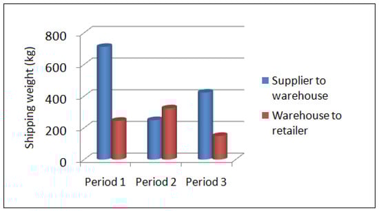 Figure 3. Shipping quantity for the periods 1, 2 and 3.
 - Deterioration rates of milk, cheese, curd, and butter are, respectively, 0, 0.01, 0.01, and 0.01 at the warehouse, whereas those of retailers are 0.0095, 0, 0, and 0, respectively. Hence, it can be concluded that more deterioration rate of the product that occurred at the warehouse in the first period, but the total deterioration rate is very low, which is more beneficial to the organization.
- Furthermore, the discount rate on transportation cost for shipping the quantities from source supplier to warehouse as well as warehouse to retailer is 0%; i.e., there is no discount on transportation cost in the first period.
- Excess weights of quantities than the weight of the full truck transported from the warehouse to retailer are 140.25 kgs, 223.7 kgs, and 19.45 kgs for periods 1, 2, and 3, respectively, in the evening.
- Figure 3 shows that the shipping weight in period 2 from warehouse to retailer is greater than the weight from supplier to warehouse.
- The remaining solutions for the rest periods 2 and 3 are depicted in Appendix A.
- Figure 4 represents the sensitivity analysis of some model’s parameters by changing their values from –50% to +50%. From that figure, it can be concluded that due to increasing of the values of truck capacity, weight of products, and transportation cost in LTL mode, the total supply chain cost increases.
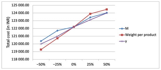 Figure 4. Effect of changes in values of parameters on total cost.
6. Main Findings and Conclusions
This research started with a clear problem of the higher cost incurred by the organization under consideration. The organization as a leading organization faces multiple competitive challenges, so staying ahead in the competition means saving on all major fronts along with the provision of the best supply system scenario. When researchers approached the problem as a multiobjective mixed integer fuzzy nonlinear programming model to minimize the total cost of the organization from our perspective, we found that the cost of the organization incurred at three different echelons and applied multiple case scenarios as shown in the analysis is less than the actual cost of the organization, which is referred to in Section 4.1. The model is first converted to a multi-objective mixed integer crisp non-linear model by using the ranking index theory discussed in Section 4.2.4 and then the multi-objective crisp model transferred into a single objective model by FNLP problem as shown in Section 4.2.5. Finally, the converted single-objective problem is solved by using a programming approach on Lingo 18.0 software. From the results, it is observed that the rate of deterioration is highest at the warehouse facilities for which the organization must update its infrastructural facilities. With a growing demand for more innovative dairy products such as flavored yogurt, lassies, or ice cream, the companies have started using Head-Induced Flavors (from pasteurization, refrigerator storage, autoclaves, high-temperature processing), light-induced flavor, oxidized flavor, and transmitted flavors, which eventually have higher deterioration rate if not kept under proper climatic controlled places. The traditional warehouses are equipped with facilities for storage of normal dairy and related products having a low deterioration rate. This realization came to the researchers as well as the organization, and hence it proved to be a learning point for both parties.
Furthermore, the deterioration can be checked at the supplier end by replacing the faulty packages with the fresh one to eliminate the deterioration risk and to reduce the holding cost at the warehouse. The deterioration rate at the retailer end also can be checked by removing the spoilage packets to diminish the holding cost and it can be managed by streamlining the demand for milk products.
We can say that our result based on fuzzy concept is similar to yet different from work done by Pal et al. [] which is based on the application of a Real-Coded Genetic Algorithm (RCGA) for mixed integer non-linear programming in a two-warehouse inventory control problem. Our model is a multiobjective mixed integer fuzzy nonlinear programming model based on two-stage supply chain framework which points towards finite horizon and finite time problems with uncertain day demand, uncertain holding cost, and uncertain purchased price at the retailer and these uncertainties are handled using a triangular fuzzy number and ranking index of a triangular fuzzy number.
Finally, it can be said that we have able to reduce the total cost of the organization, and this is the main contribution of the present study. So, to tackle the uncertain situation, the fuzzy concept will be beneficial to any organization.
7. Limitations and Future Scope
This study is restricted to the national capital region only and focuses on the parameters of certain demands and time and has covered only a limited period of a year. For future studies, the models can be replicated for uncertain demand for all products and time, uncertain periods, multi-echelon, multi-item supply chain, and covering different locations for parts of India seeking suitability for the hub-and-spoke model. Furthermore, this study can be extended by using two-fold uncertain (intuitionistic/rough) environment to handle the uncertainty in demand, holding cost, etc. One may solve the proposed multi-objective nonlinear programming problem by applying the intuitionistic fuzzy TOPSIS approach to obtain the required optimal solution from a deterministic multiobjective mixed integer nonlinear programming problem. The proposed study is suitable for dealing with the uncertainties in delivery in the disaster situation of COVID-19.
Author Contributions
S.S.A.: Concept building, data collection, model building, assumptions and formulation validation, lead-supervision and compilation of various sections; H.B.: Formulation and analysis; R.K.: Compilation of various sections; H.T.: Proof reading and formatting; S.K.R.: Analysis and formulation supervision. All authors have read and agreed to the published version of the manuscript.
Funding
The authors are indebted to the stated organization for providing valuable data for carrying out this research. We express our deepest gratitude to the team members at New Delhi Center for their insight and expertise about specific information related to uncertain situations and route problems that greatly assisted our research. This project was funded by the Deanship of Scientific Research (DSR) at King Abdulaziz University, Jeddah, under grant no. D-016-144-1440. The authors, therefore, acknowledge with thanks DSR for technical and financial support. Haripriya Barman is very much thankful to University Grants Commission (UGC) of India for providing financial support to continue this research work under Junior Research Fellowship scheme with UGC-reference number: [UGC-Ref.No.: 1166/(CSIR-UGC NET DEC.2017)] dated 8 February 2019.
Institutional Review Board Statement
Not applicable.
Informed Consent Statement
Not applicable.
Acknowledgments
The authors are indebted to the stated organization for providing valuable data for carrying out this research. We express our deepest gratitude to the team members at New Delhi centers for their insight and expertise about specific information related to uncertain situations and route problems that greatly assisted our research. This work was supported by the Deanship of Scientific Research (DSR), King Abdulaziz University, Jeddah, under grant no. (D-016-144-1440). The authors, therefore, gratefully acknowledge the DSR technical and financial support. This work has been partially supported by the Faculty of Informatics and Management UHK specific research project 2107 Integration of Departmental Research Activities and Students’ Research Activities Support. The authors would like to express their thanks to student D. Sec for contributing to this topic.
Conflicts of Interest
The authors declare no conflict of interest.
Appendix A
Table A1.
Quantity and purchase cost of four products at suppliers.
Table A1.
Quantity and purchase cost of four products at suppliers.
| Product | Purchase Quantity | Purchase Cost (Rupees) | |
|---|---|---|---|
| P I | Milk | 850 g | 47, 48, 49 |
| P II | Cheese | 200 g | 60, 62, 67 |
| P III | Curd | 650 g | 51, 54, 60 |
| P IV | Butter | 550 g | 105, 110, 120 |
Table A2.
Initial quantity and inspection cost per packet of four products at retailers.
Table A2.
Initial quantity and inspection cost per packet of four products at retailers.
| Product | Initial Inventory at Destination (Packets) | Inspection Cost per Packet (Rupees) | |
|---|---|---|---|
| P I | Milk | 88 | 1 |
| P II | Cheese | 84 | |
| P III | Curd | 80 | |
| P IV | Butter | 83 |
Table A3.
Holding cost at warehouse.
Table A3.
Holding cost at warehouse.
| Product | Period I | Period II | Period III | |
|---|---|---|---|---|
| P I | Milk | 2, 3, 3.9 | 2, 2.5, 2.7 | 2.5, 2.7, 3 |
| P II | Cheese | 1.5, 2, 2.6 | 2.1, 2.5, 2.6 | 2.4, 2.6, 3.5 |
| P III | Curd | 1.5, 2, 2.4 | 2.3, 2.5, 3 | 3, 3.4, 3.8 |
| P IV | Butter | 1.6, 2, 2.4 | 2, 2.5, 1.8 | 2.8, 3, 3.5 |
Table A4.
Holding cost at destination/retailers.
Table A4.
Holding cost at destination/retailers.
| Product | Period I | Period II | Period III | |
|---|---|---|---|---|
| P I | Milk | 2.5, 3.2, 3.1 | 3.3, 3, 3.7 | 3, 3.5, 2.8 |
| P II | Cheese | 2, 2.3, 2.9 | 2.6, 3, 3.5 | 3, 2.6, 3.1 |
| P III | Curd | 2.3, 2.8, 2.1 | 3.4, 2.3, 3.5 | 3, 3.8, 3.4 |
| P IV | Butter | 2, 2.4, 2.6 | 2.7, 2.5, 2.9 | 3.9, 3.5, 3.1 |
Table A5.
Total demand for four products at retailers.
Table A5.
Total demand for four products at retailers.
| Product | Period I | Period II | Period III | |
|---|---|---|---|---|
| P I | Milk | 140-M * and 152-E * | 170-M and 180-E | 190-M and 180-E |
| P II | Cheese | 139, 145, 154 | 185, 190, 200 | 186, 187, 191 |
| P III | Curd | 179, 180, 181 | 175, 176, 180 | 187, 188, 195 |
| P IV | Butter | 165, 169, 164 | 180, 182, 184 | 190, 188, 176 |
* M and E refer to morning and evening.
Table A6.
Holding and Halting Cost per 100 kg weight in road.
Table A6.
Holding and Halting Cost per 100 kg weight in road.
| Cost (First Day) | Cost (Second Day on Wards) | |
|---|---|---|
| Period I | 7 | 2 |
| Period II | 8 | 3 |
| Period III | 9 | 4 |
Table A7.
Transportation cost for full truck without uncertainty.
Table A7.
Transportation cost for full truck without uncertainty.
| Time Frame | Cost (Rupees) |
|---|---|
| Period I | 1500 |
| Period II | 1650 |
| Period III | 1700 |
Table A8.
Quantity threshold and discount factor for PI and PII for all periods.
Table A8.
Quantity threshold and discount factor for PI and PII for all periods.
| Quantity Threshold | Discount Factor | Quantity Threshold | Discount Factor |
|---|---|---|---|
| PI | PI | PII | PII |
| 0–100 | 1 | 0–145 | 1 |
| 100–200 | 0.97 | 145–180 | 0.93 |
| 200–300 | 0.94 | 180–220 | 0.91 |
| 300 & above | 0.9 | 220 & above | 0.87 |
Table A9.
Quantity threshold and discount factor for PIII and PIV for all periods.
Table A9.
Quantity threshold and discount factor for PIII and PIV for all periods.
| Quantity Threshold | Discount Factor | Quantity Threshold | Discount Factor |
|---|---|---|---|
| PIII | PIII | PIV | PIV |
| 0–136 | 1 | 0–110 | 1 |
| 136–170 | 0.97 | 110–140 | 0.95 |
| 170–230 | 0.94 | 140–190 | 0.92 |
| 230 & above | 0.9 | 190 & above | 0.9 |
Table A10.
Weight threshold and discount factors for all periods (transportation).
Table A10.
Weight threshold and discount factors for all periods (transportation).
| Weight Threshold | Discount Factors |
|---|---|
| 100–400 | 1 |
| 400–700 | 0.97 |
| 700–1000 | 0.94 |
| 1000 & above | 0.91 |
Table A11.
Consumption at destination/retailers.
Table A11.
Consumption at destination/retailers.
| Product | Period I | Period II | Period III | |
|---|---|---|---|---|
| P I | Milk | 140 | 170 | 185 |
| P II | Cheese | 132 | 155 | 180 |
| P III | Curd | 170 | 200 | 171 |
| P IV | Butter | 170 | 120 | 175 |
Table A12.
Solution of our proposed model from supplier to warehouse.
Table A12.
Solution of our proposed model from supplier to warehouse.
| Product | Discount on Purchased Cost | Discount on Transportation Cost | |||||
|---|---|---|---|---|---|---|---|
| In period 1 from source supplier to warehouse | |||||||
| 1 | 544 | 339 | 0 | 10% | 0% | ||
| 2 | 386 | 146 | 3 | 1 | 0.01 | 13% | |
| 3 | 103 | 3 | 0.01 | 0% | |||
| 4 | 190 | 0 | 0.01 | 10% | |||
| In period 2 from source supplier to warehouse | |||||||
| 1 | 3 | 0 | 0.01 | 0% | 0% | ||
| 2 | 0 | 146 | 1 | 1 | 0 | 0% | |
| 3 | 208 | 2 | 0.01 | 0% | |||
| 4 | 202 | 123 | 0 | 10% | |||
| In period 3 from source supplier to warehouse | |||||||
| 1 | 370 | 0 | 0.01 | 10% | 0% | ||
| 2 | 0 | 0 | 2 | 2 | 0.01 | 0% | |
| 3 | 166 | 0 | 0.01 | 0% | |||
| 4 | 0 | 0 | 0.01 | 0% | |||
Table A13.
Solution of our proposed model part 2.
Table A13.
Solution of our proposed model part 2.
| Product | ||||||
|---|---|---|---|---|---|---|
| In period 1 from warehouse to retailer | ||||||
| 1 | 381 | 651 | 2 | 0.0095 | 1 | 140.883 |
| 2 | 239 | 119 | 1 | 0 | 0 | |
| 3 | 100 | 11 | 0 | 0 | 0 | |
| 4 | 190 | 110 | 3 | 0 | 0 | |
| In period 2 from warehouse to retailer | ||||||
| 1 | 80 | 262 | 0 | 0 | 1 | 223.34 |
| 2 | 0 | 41 | 1 | 0 | 0 | |
| 3 | 212 | 22 | 1 | 0 | 0 | |
| 4 | 79 | 62 | 1 | 0 | 0 | |
| In period 3 from warehouse to retailer | ||||||
| 1 | 52 | 317 | 1 | 0 | 1 | 19.45 |
| 2 | 9 | 0 | 0 | 0 | 0 | |
| 3 | 161 | 0 | 2 | 0 | 0 | |
| 4 | 0 | 0 | 0 | 0 | 0 | |
References
- Dye, C.Y.; Hsieh, T.P.; Ouyang, L.Y. Determining optimal selling price and lot size with a varying rate of deterioration and exponential partial backlogging. Eur. J. Oper. Res. 2007, 181, 668–678. [Google Scholar] [CrossRef]
- Blackburn, J.; Scudder, G. Supply chain strategies for perishable products: The case of fresh produce. Prod. Oper. Manag. 2009, 18, 129–137. [Google Scholar] [CrossRef]
- Paksoy, T.; Kochan, C.G.; Ali, S.S. Logistics 4.0: Digital Transformation of Supply Chain Management; CRC Press: Boca Raton, FL, USA, 2020. [Google Scholar]
- Bakker, M.; Riezebos, J.; Teunter, R.H. Review of inventory systems with deterioration since 2001. Eur. J. Oper. Res. 2012, 221, 275–284. [Google Scholar] [CrossRef]
- Goyal, S.K.; Giri, B.C. Recent trends in modeling of deteriorating inventory. Eur. J. Oper. Res. 2001, 134, 1–16. [Google Scholar] [CrossRef]
- Dobson, G.; Pinker, E.J.; Yildiz, O. An EOQ model for perishable goods with age-dependent demand rate. Eur. J. Oper. Res. 2017, 257, 84–88. [Google Scholar] [CrossRef]
- Hasani, A.; Zegordi, S.H.; Nikbakhsh, E. Robust closed-loop supply chain network design for perishable goods in agile manufacturing under uncertainty. Int. J. Prod. Res. 2012, 50, 4649–4669. [Google Scholar] [CrossRef]
- Janssen, E.; Sriver, R.; Wuebbles, D.J.; Kunkel, K. Seasonal and regional variations in extreme precipitation event frequency using CMIP5. Geophys. Res. Lett. 2016, 43, 5385–5393. [Google Scholar] [CrossRef]
- Pahl, J.; Voß, S. Integrating deterioration and lifetime constraints in production and supply chain planning: A survey. Eur. J. Oper. Res. 2014, 238, 654–674. [Google Scholar] [CrossRef]
- Gunasekaran, A.; Patel, C.; Tirtiroglu, E. Performance measures and metrics in a supply chain environment. Int. J. Oper. Prod. Manag. 2001, 21, 71–87. [Google Scholar] [CrossRef]
- Webster, M. Supply system structure, management and performance: A conceptual model. Int. J. Manag. Rev. 2002, 4, 353–369. [Google Scholar] [CrossRef]
- Evans, A. The Feeding of the Nine Billion: Global Food Security for the 21st Century; Chatham Historical Society Incorporated: Suffolk County, NY, USA, 2009. [Google Scholar]
- Liu, L.; Liu, X.; Liu, G. The risk management of perishable supply chain based on coloured Petri Net modeling. Inf. Process. Agric. 2018, 5, 47–59. [Google Scholar] [CrossRef]
- Elrod, C.; Murray, S.; Bande, S. A review of performance metrics for supply chain management. Eng. Manag. J. 2013, 25, 39–50. [Google Scholar] [CrossRef]
- Pahl, J.; Voß, S.; Woodruff, D.L. Production planning with load dependent lead times: An update of research. Ann. Oper. Res. 2007, 153, 297–345. [Google Scholar] [CrossRef]
- Ferguson, M.E.; Koenigsberg, O. How should a firm manage deteriorating inventory? Prod. Oper. Manag. 2007, 16, 306–321. [Google Scholar] [CrossRef]
- Gunasekaran, A.; Subramanian, N.; Rahman, S. Supply chain resilience: Role of complexities and strategies. Int. J. Prod. Res. 2015, 53. [Google Scholar] [CrossRef]
- Bernardo, J.J.; Mohamed, Z. The measurement and use of operational flexibility in the loading of flexible manufacturing systems. Eur. J. Oper. Res. 1992, 60, 144–155. [Google Scholar] [CrossRef]
- Gupta, Y.P.; Goyal, S. Flexibility of manufacturing systems: Concepts and measurements. Eur. J. Oper. Res. 1989, 43, 119–135. [Google Scholar] [CrossRef]
- Gupta, Y.P.; Somers, T.M. The measurement of manufacturing flexibility. Eur. J. Oper. Res. 1992, 60, 166–182. [Google Scholar] [CrossRef]
- Koste, L.L.; Malhotra, M.K. A theoretical framework for analyzing the dimensions of manufacturing flexibility. J. Oper. Manag. 1999, 18, 75–93. [Google Scholar] [CrossRef]
- Vokurka, R.J.; O’Leary-Kelly, S.W. A review of empirical research on manufacturing flexibility. J. Oper. Manag. 2000, 18, 485–501. [Google Scholar] [CrossRef]
- Duclos, L.K.; Vokurka, R.J.; Lummus, R.R. A conceptual model of supply chain flexibility. Ind. Manag. Data Syst. 2003, 103, 446–456. [Google Scholar] [CrossRef]
- Pujawan, I.N. Assessing supply chain flexibility: A conceptual framework and case study. Int. J. Integr. Supply Manag. 2004, 1, 79–97. [Google Scholar] [CrossRef]
- Gong, Z. An economic evaluation model of supply chain flexibility. Eur. J. Oper. Res. 2008, 184, 745–758. [Google Scholar] [CrossRef]
- Nahmias, S. Perishable inventory theory: A review. Oper. Res. 1982, 30, 680–708. [Google Scholar] [CrossRef] [PubMed]
- Ghare, P. A model for an exponentially decaying inventory. J. Ind. Eng. 1963, 14, 238–243. [Google Scholar]
- Van Zyl, G.J. Inventory Control for Perishable Commodities; Technical Report; North Carolina State University: Raleigh, NC, USA, 1963. [Google Scholar]
- Friedman, Y.; Hoch, Y. A dynamic lot-size model with inventory deterioration. INFOR Inf. Syst. Oper. Res. 1978, 16, 183–188. [Google Scholar] [CrossRef]
- Covert, R.P.; Philip, G.C. An EOQ model for items with Weibull distribution deterioration. AIIE Trans. 1973, 5, 323–326. [Google Scholar] [CrossRef]
- Goswami, A.; Chaudhuri, K. Variations of order-level inventory models for deteriorating items. Int. J. Prod. Econ. 1992, 27, 111–117. [Google Scholar] [CrossRef]
- Bose, S.; Goswami, A.; Chaudhuri, K. An EOQ model for deteriorating items with linear time-dependent demand rate and shortages under inflation and time discounting. J. Oper. Res. Soc. 1995, 46, 771–782. [Google Scholar] [CrossRef]
- Barman, H.; Pervin, M.; Roy, S.K.; Weber, G.W. Back-ordered inventory model with inflation in a cloudy-fuzzy environment. J. Ind. Manag. Optim. 2021, 17, 1913–1941. [Google Scholar] [CrossRef]
- Hsu, V.N. Dynamic economic lot size model with perishable inventory. Manag. Sci. 2000, 46, 1159–1169. [Google Scholar] [CrossRef]
- Pervin, M.; Roy, S.K.; Weber, G.W. Analysis of inventory control model with shortage under time-dependent demand and time-varying holding cost including stochastic deterioration. Ann. Oper. Res. 2018, 260, 437–460. [Google Scholar] [CrossRef]
- Pervin, M.; Roy, S.K.; Weber, G.W. Multi-item deteriorating two-echelon inventory model with price-and stock-dependent demand: A trade-credit policy. J. Ind. Manag. Optim. 2019, 15, 1345–1373. [Google Scholar] [CrossRef]
- Lütke Entrup, M.; Günther, H.O.; Van Beek, P.; Grunow, M.; Seiler, T. Mixed-Integer Linear Programming approaches to shelf-life-integrated planning and scheduling in yoghurt production. Int. J. Prod. Res. 2005, 43, 5071–5100. [Google Scholar] [CrossRef]
- Mishra, V.K. An inventory model of instantaneous deteriorating items with controllable deterioration rate for time dependent demand and holding cost. J. Ind. Eng. Manag. (JIEM) 2013, 6, 496–506. [Google Scholar] [CrossRef]
- Hou, K.L.; Lin, L.C. An EOQ model for deteriorating items with price-and stock-dependent selling rates under inflation and time value of money. Int. J. Syst. Sci. 2006, 37, 1131–1139. [Google Scholar] [CrossRef]
- Jans, R.; Degraeve, Z. Modeling industrial lot sizing problems: A review. Int. J. Prod. Res. 2008, 46, 1619–1643. [Google Scholar] [CrossRef]
- Teng, J.T.; Krommyda, I.P.; Skouri, K.; Lou, K.R. A comprehensive extension of optimal ordering policy for stock-dependent demand under progressive payment scheme. Eur. J. Oper. Res. 2011, 215, 97–104. [Google Scholar] [CrossRef]
- Chowdhury, R.R.; Ghosh, S.; Chaudhuri, K. An inventory model for deteriorating items with stock and price sensitive demand. Int. J. Appl. Comput. Math. 2015, 1, 187–201. [Google Scholar] [CrossRef][Green Version]
- Chang, C.T.; Cheng, M.C.; Ouyang, L.Y. Optimal pricing and ordering policies for non-instantaneously deteriorating items under order-size-dependent delay in payments. Appl. Math. Model. 2015, 39, 747–763. [Google Scholar] [CrossRef]
- Wang, K.J.; Lin, Y.S. Optimal inventory replenishment strategy for deteriorating items in a demand-declining market with the retailer’s price manipulation. Ann. Oper. Res. 2012, 201, 475–494. [Google Scholar] [CrossRef]
- Herbon, A. Optimal two-level piecewise-constant price discrimination for a storable perishable product. Int. J. Prod. Res. 2018, 56, 1738–1756. [Google Scholar] [CrossRef]
- Dye, C.Y.; Hsieh, T.P. Joint pricing and ordering policy for an advance booking system with partial order cancellations. Appl. Math. Model. 2013, 37, 3645–3659. [Google Scholar] [CrossRef]
- Ali, S.S.; Madaan, J.; Chan, F.T.; Kannan, S. Inventory management of perishable products: A time decay linked logistic approach. Int. J. Prod. Res. 2013, 51, 3864–3879. [Google Scholar] [CrossRef]
- Soni, H.N. Optimal replenishment policies for non-instantaneous deteriorating items with price and stock sensitive demand under permissible delay in payment. Int. J. Prod. Econ. 2013, 146, 259–268. [Google Scholar] [CrossRef]
- Tayal, S.; Singh, S.; Sharma, R.; Chauhan, A. Two echelon supply chain model for deteriorating items with effective investment in preservation technology. Int. J. Math. Oper. Res. 2014, 6, 84–105. [Google Scholar] [CrossRef]
- Chung, W.; Talluri, S.; Narasimhan, R. Optimal pricing and inventory strategies with multiple price markdowns over time. Eur. J. Oper. Res. 2015, 243, 130–141. [Google Scholar] [CrossRef]
- Raiconi, A.; Pahl, J.; Gentili, M.; Voß, S.; Cerulli, R. Tactical Production and Lot Size Planning with Lifetime Constraints: A Comparison of Model Formulations. Asia-Pac. J. Oper. Res. 2017, 34, 1750019. [Google Scholar] [CrossRef]
- Tai, A.H.; Xie, Y.; Ching, W.K. Inspection policy for inventory system with deteriorating products. Int. J. Prod. Econ. 2016, 173, 22–29. [Google Scholar] [CrossRef]
- Karmakar, B.; Choudhury, K.D. A review on inventory models for deteriorating items with shortages. Assam Univ. J. Sci. Technol. 2010, 6, 51–59. [Google Scholar]
- Li, X.; Zhu, Y.; Zhang, Z. An LCA-based environmental impact assessment model for construction processes. Build. Environ. 2010, 45, 766–775. [Google Scholar] [CrossRef]
- Karaesmen, I.Z.; Scheller-Wolf, A.; Deniz, B. Managing perishable and aging inventories: Review and future research directions. Plan. Prod. Invent. Ext. Enterp. 2011, 151, 393–436. [Google Scholar]
- Chen, J.; Chen, L. Pricing and lot-sizing for a deteriorating item in a periodic review inventory system with shortages. J. Oper. Res. Soc. 2004, 55, 892–901. [Google Scholar] [CrossRef]
- Amorim, P.; Antunes, C.H.; Almada-Lobo, B. Multi-objective lot-sizing and scheduling dealing with perishability issues. Ind. Eng. Chem. Res. 2011, 50, 3371–3381. [Google Scholar] [CrossRef]
- Van Kampen, T.J.; Van Donk, D.P.; Van Der Zee, D.J. Safety stock or safety lead time: Coping with unreliability in demand and supply. Int. J. Prod. Res. 2010, 48, 7463–7481. [Google Scholar] [CrossRef]
- Chen, J.; Chen, T. Effects of joint replenishment and channel coordination for managing multiple deteriorating products in a supply chain. J. Oper. Res. Soc. 2005, 56, 1224–1234. [Google Scholar] [CrossRef]
- Balkhi, Z.T.; Tadj, L. A generalized economic order quantity model with deteriorating items and time varying demand, deterioration, and costs. Int. Trans. Oper. Res. 2008, 15, 509–517. [Google Scholar] [CrossRef]
- Chern, M.S.; Chan, Y.L.; Teng, J.T. A comparison among various inventory shortage models for deteriorating items on the basis of maximizing profit. Asia-Pac. J. Oper. Res. 2005, 22, 121–134. [Google Scholar] [CrossRef]
- Skouri, K.; Papachristos, S. Four inventory models for deteriorating items with time varying demand and partial backlogging: A cost comparison. Optim. Control Appl. Methods 2003, 24, 315–330. [Google Scholar] [CrossRef]
- Wu, J.; Chang, C.T.; Cheng, M.C.; Teng, J.T.; Al-khateeb, F.B. Inventorymanagement for fresh produce when the time-varying demand depends on product freshness, stock level and expiration date. Int. J. Syst. Sci. Oper. Logist. 2016, 3, 138–147. [Google Scholar] [CrossRef]
- Bhunia, A.; Shaikh, A. A deterministic model for deteriorating items with displayed inventory level dependent demand rate incorporating marketing decisions with transportation cost. Int. J. Ind. Eng. Comput. 2011, 2, 547–562. [Google Scholar] [CrossRef]
- Jolai, F.; Tavakkoli-Moghaddam, R.; Rabbani, M.; Sadoughian, M. An economic production lot size model with deteriorating items, stock-dependent demand, inflation, and partial backlogging. Appl. Math. Comput. 2006, 181, 380–389. [Google Scholar] [CrossRef]
- Pal, A.; Bhunia, A.K.; Mukherjee, R. Optimal lot size model for deteriorating items with demand rate dependent on displayed stock level (DSL) and partial backordering. Eur. J. Oper. Res. 2006, 175, 977–991. [Google Scholar] [CrossRef]
- Liu, G.; Zhang, J.; Tang, W. Joint dynamic pricing and investment strategy for perishable foods with price-quality dependent demand. Ann. Oper. Res. 2015, 226, 397–416. [Google Scholar] [CrossRef]
- Qin, Y.; Wang, J.; Wei, C. Joint pricing and inventory control for fresh produce and foods with quality and physical quantity deteriorating simultaneously. Int. J. Prod. Econ. 2014, 152, 42–48. [Google Scholar] [CrossRef]
- Guchhait, P.; Maiti, M.K.; Maiti, M. An EOQ model of deteriorating item in imprecise environment with dynamic deterioration and credit linked demand. Appl. Math. Model. 2015, 39, 6553–6567. [Google Scholar] [CrossRef]
- Mahata, G.C. Retailer’s optimal credit period and cycle time in a supply chain for deteriorating items with up-stream and down-stream trade credits. J. Ind. Eng. Int. 2015, 11, 353–366. [Google Scholar] [CrossRef]
- Shah, N.H.; Cárdenas-Barrón, L.E. Retailer’s decision for ordering and credit policies for deteriorating items when a supplier offers order-linked credit period or cash discount. Appl. Math. Comput. 2015, 259, 569–578. [Google Scholar] [CrossRef]
- Singh, S.; Sharma, S. A global optimizing policy for decaying items with ramp-type demand rate under two-level trade credit financing taking account of preservation technology. Adv. Decis. Sci. 2013, 2013, 126385. [Google Scholar] [CrossRef]
- Feng, L.; Chan, Y.L.; Cárdenas-Barrón, L.E. Pricing and lot-sizing polices for perishable goods when the demand depends on selling price, displayed stocks, and expiration date. Int. J. Prod. Econ. 2017, 185, 11–20. [Google Scholar] [CrossRef]
- Xue, M.; Tang, W.; Zhang, J. Optimal dynamic pricing for deteriorating items with reference-price effects. Int. J. Syst. Sci. 2016, 47, 2022–2031. [Google Scholar] [CrossRef]
- Jain, D.; Aggarwal, K.K. The effect of inflation-induced demand and trade credit on ordering policy of exponentially deteriorating and imperfect quality items. Int. Trans. Oper. Res. 2012, 19, 863–889. [Google Scholar] [CrossRef]
- Kaminsky, P.; Simchi-Levi, D. Production and distribution lot sizing in a two stage supply chain. IIE Trans. 2003, 35, 1065–1075. [Google Scholar] [CrossRef]
- Hwang, H.S. A stochastic set-covering location model for both ameliorating and deteriorating items. Comput. Ind. Eng. 2004, 46, 313–319. [Google Scholar] [CrossRef]
- Yang, H.L. Two-warehouse inventory models for deteriorating items with shortages under inflation. Eur. J. Oper. Res. 2004, 157, 344–356. [Google Scholar] [CrossRef]
- Ahn, H.S.; Kaminsky, P. Production and distribution policy in a two-stage stochastic push-pull supply chain. IIE Trans. 2005, 37, 609–621. [Google Scholar] [CrossRef]
- Pal, P.; Das, C.; Panda, A.; Bhunia, A.K. An application of real-coded genetic algorithm (for mixed integer non-linear programming in an optimal two-warehouse inventory policy for deteriorating items with a linear trend in demand and a fixed planning horizon). Int. J. Comput. Math. 2005, 82, 163–175. [Google Scholar] [CrossRef]
- Rieksts, B.Q.; Ventura, J.A. Two-stage inventory models with a bi-modal transportation cost. Comput. Oper. Res. 2010, 37, 20–31. [Google Scholar] [CrossRef]
- Hwang, H.; Moon, D.H.; Shinn, S.W. An EOQ model with quantity discounts for both purchasing price and freight cost. Comput. Oper. Res. 1990, 17, 73–78. [Google Scholar] [CrossRef]
- Ertogral, K. Multi-item single source ordering problem with transportation cost: A Lagrangian decomposition approach. Eur. J. Oper. Res. 2008, 191, 156–165. [Google Scholar] [CrossRef]
- Mendoza, A.; Ventura, J.A. Incorporating quantity discounts to the EOQ model with transportation costs. Int. J. Prod. Econ. 2008, 113, 754–765. [Google Scholar] [CrossRef]
- Tersine, R.J.; Barman, S. Lot size optimization with quantity and freight rate discounts. Logist. Transp. Rev. 1991, 27, 319. [Google Scholar]
- Gandhi, K.; Jha, P.; Ali, S.S. A two stage EOQ model for deteriorating products incorporating quantity & freight discounts, under fuzzy environment. In Proceedings of the Seventh International Conference on Bio-Inspired Computing: Theories and Applications (BIC-TA 2012), Qingdao, China, 23–25 October 2013; pp. 367–380. [Google Scholar]
- Behzadi, G.; O’Sullivan, M.J.; Olsen, T.L.; Scrimgeour, F.; Zhang, A. Robust and resilient strategies for managing supply disruptions in an agribusiness supply chain. Int. J. Prod. Econ. 2017, 191, 207–220. [Google Scholar] [CrossRef]
- Coniglio, S.; Koster, A.M.; Spiekermann, N. Lot sizing with storage losses under demand uncertainty. J. Comb. Optim. 2018, 36, 763–788. [Google Scholar] [CrossRef]
- Brahimi, N.; Absi, N.; Dauzère-Pérès, S.; Nordli, A. Single-item dynamic lot-sizing problems: An updated survey. Eur. J. Oper. Res. 2017, 263, 838–863. [Google Scholar] [CrossRef]
- Mendel, J.M.; John, R.B. Type-2 fuzzy sets made simple. IEEE Trans. Fuzzy Syst. 2002, 10, 117–127. [Google Scholar] [CrossRef]
- Karnik, N.N.; Mendel, J.M.; Liang, Q. Type-2 fuzzy logic systems. IEEE Trans. Fuzzy Syst. 1999, 7, 643–658. [Google Scholar] [CrossRef]
- Ali, S.S.; Paksoy, T.; Torğul, B.; Kaur, R. Reverse logistics optimization of an industrial air conditioner manufacturing company for designing sustainable supply chain: A fuzzy hybrid multi-criteria decision-making approach. Wirel. Netw. 2020, 26, 5759–5782. [Google Scholar] [CrossRef]
- Yager, R.R. A procedure for ordering fuzzy subsets of the unit interval. Inf. Sci. 1981, 24, 143–161. [Google Scholar] [CrossRef]
- Zimmermann, H.J. Fuzzy programming and linear programming with several objective functions. Fuzzy Sets Syst. 1978, 1, 45–55. [Google Scholar] [CrossRef]
Publisher’s Note: MDPI stays neutral with regard to jurisdictional claims in published maps and institutional affiliations. |
© 2021 by the authors. Licensee MDPI, Basel, Switzerland. This article is an open access article distributed under the terms and conditions of the Creative Commons Attribution (CC BY) license (https://creativecommons.org/licenses/by/4.0/).