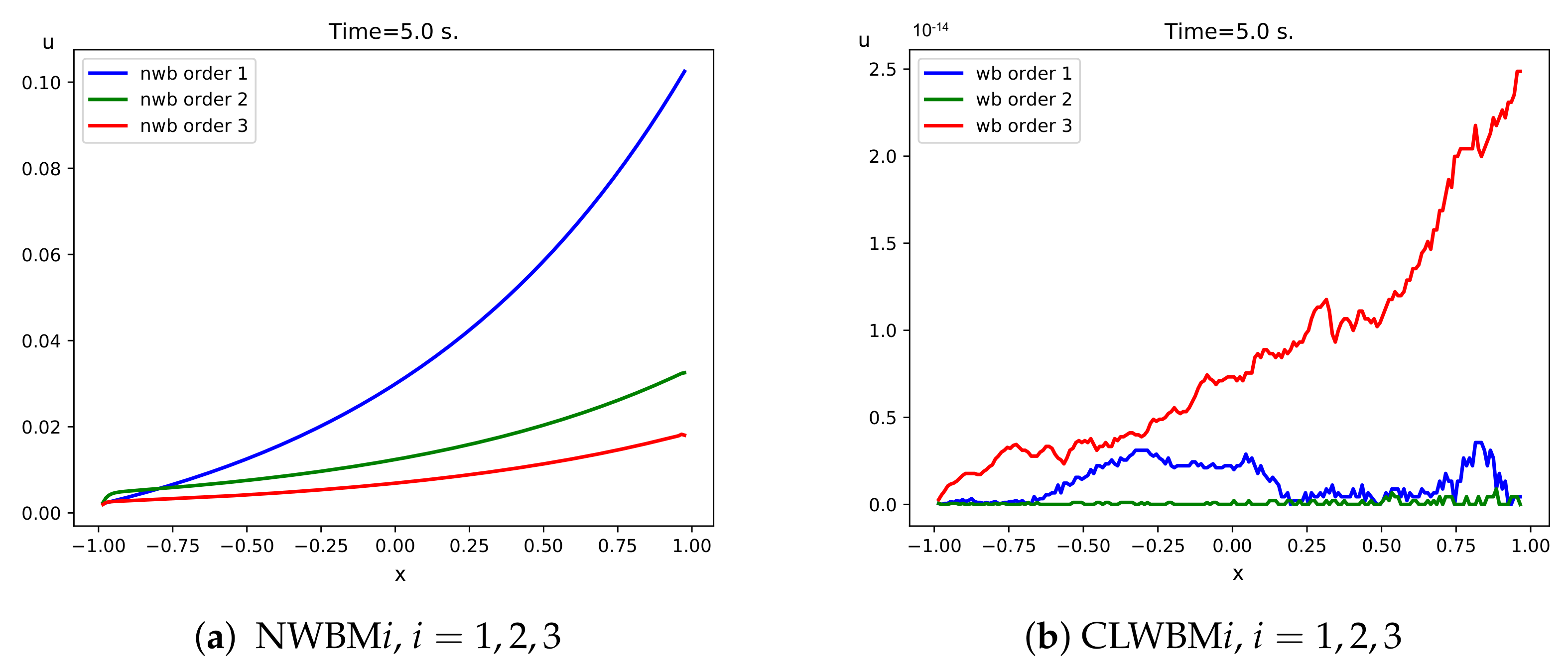
Figure 1.
Test 1.1. Differences between the stationary and the numerical solutions at time s for a 200-cell mesh.
Figure 1.
Test 1.1. Differences between the stationary and the numerical solutions at time s for a 200-cell mesh.
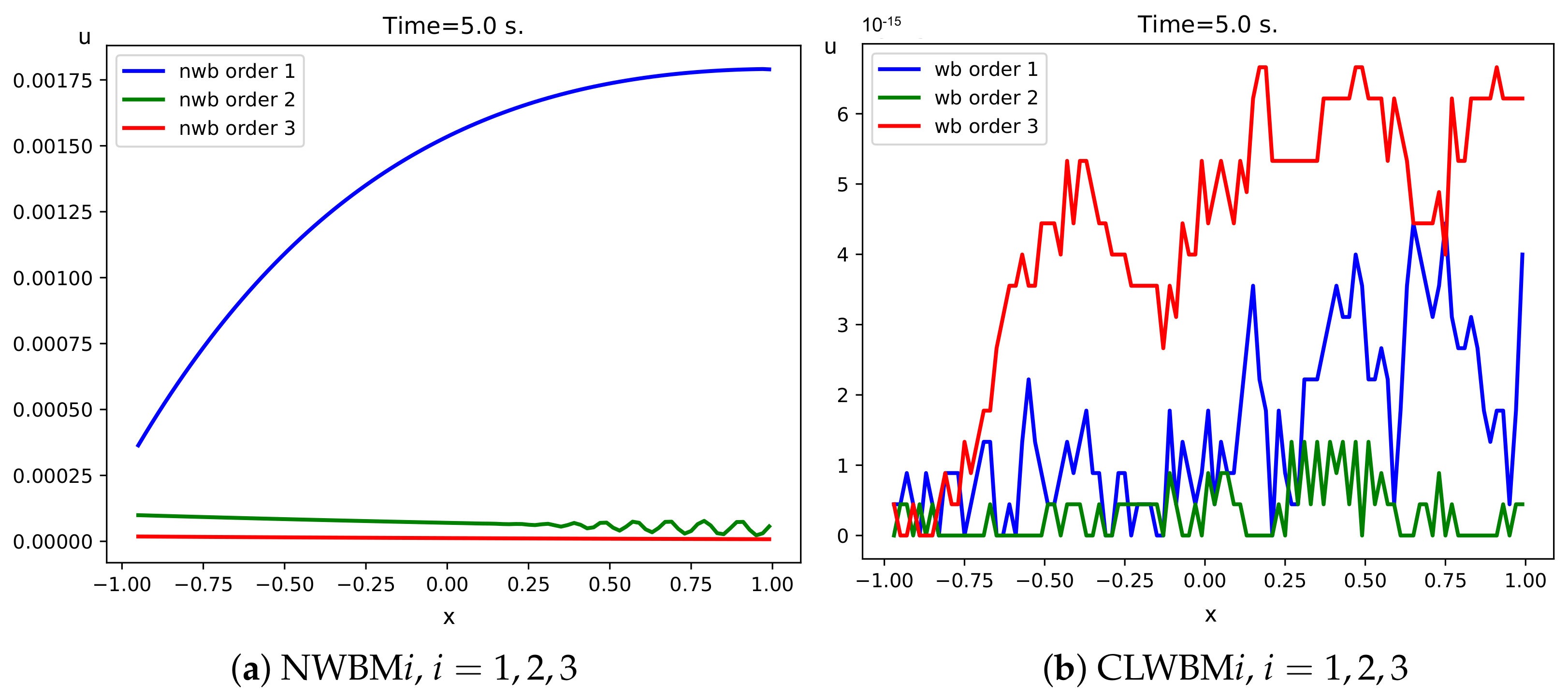
Figure 2.
Test 2.1. Differences between the stationary and the numerical solutions at s using a mesh with 100 cells.
Figure 2.
Test 2.1. Differences between the stationary and the numerical solutions at s using a mesh with 100 cells.
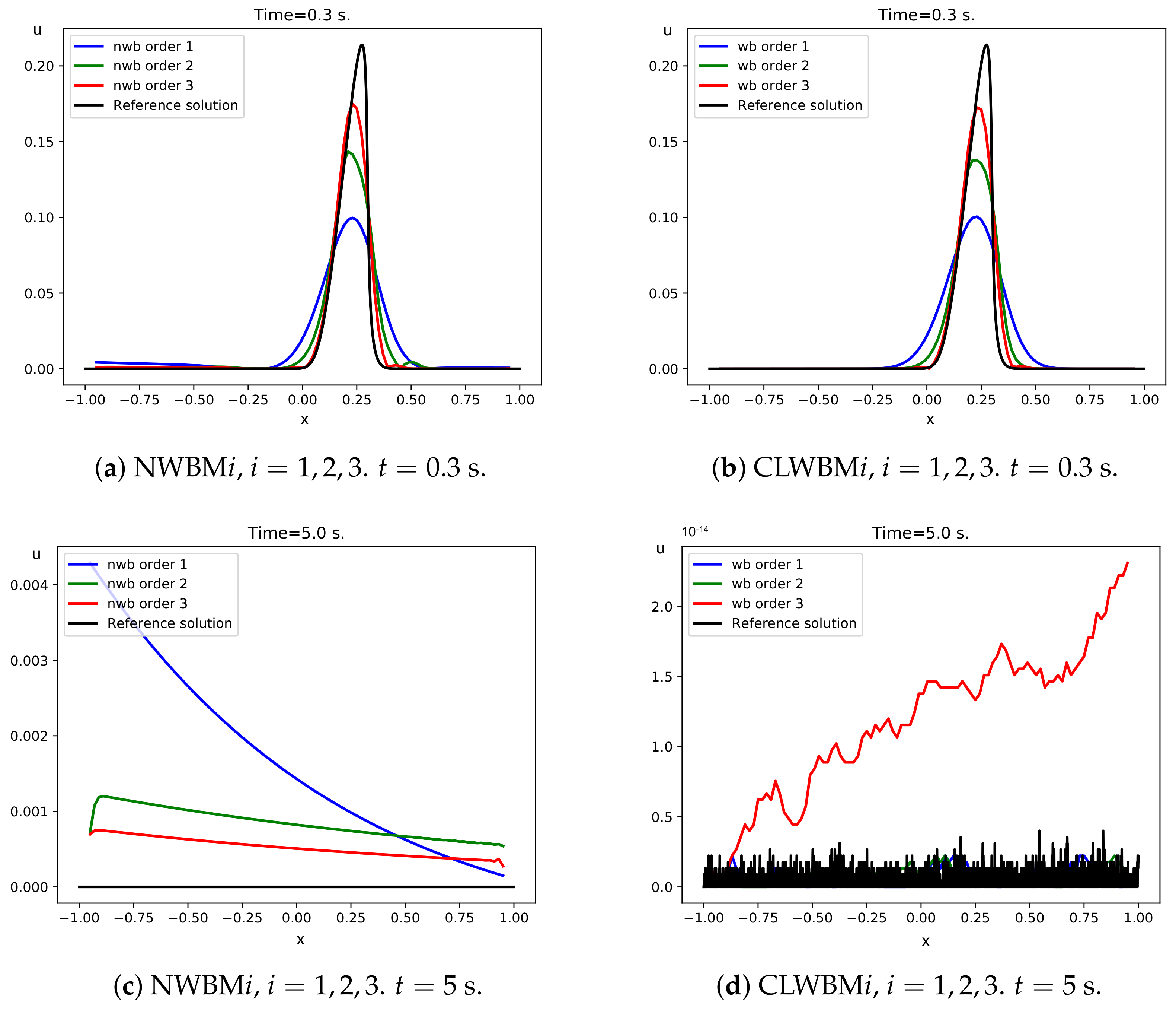
Figure 3.
Test 2.2. Reference and numerical solutions: differences with the stationary solution at times s for a 100-cell mesh.
Figure 3.
Test 2.2. Reference and numerical solutions: differences with the stationary solution at times s for a 100-cell mesh.
Figure 4.
Test 3.1. Reference and numerical solutions: differences with the stationary solution at time s for the 200-cell mesh.
Figure 4.
Test 3.1. Reference and numerical solutions: differences with the stationary solution at time s for the 200-cell mesh.
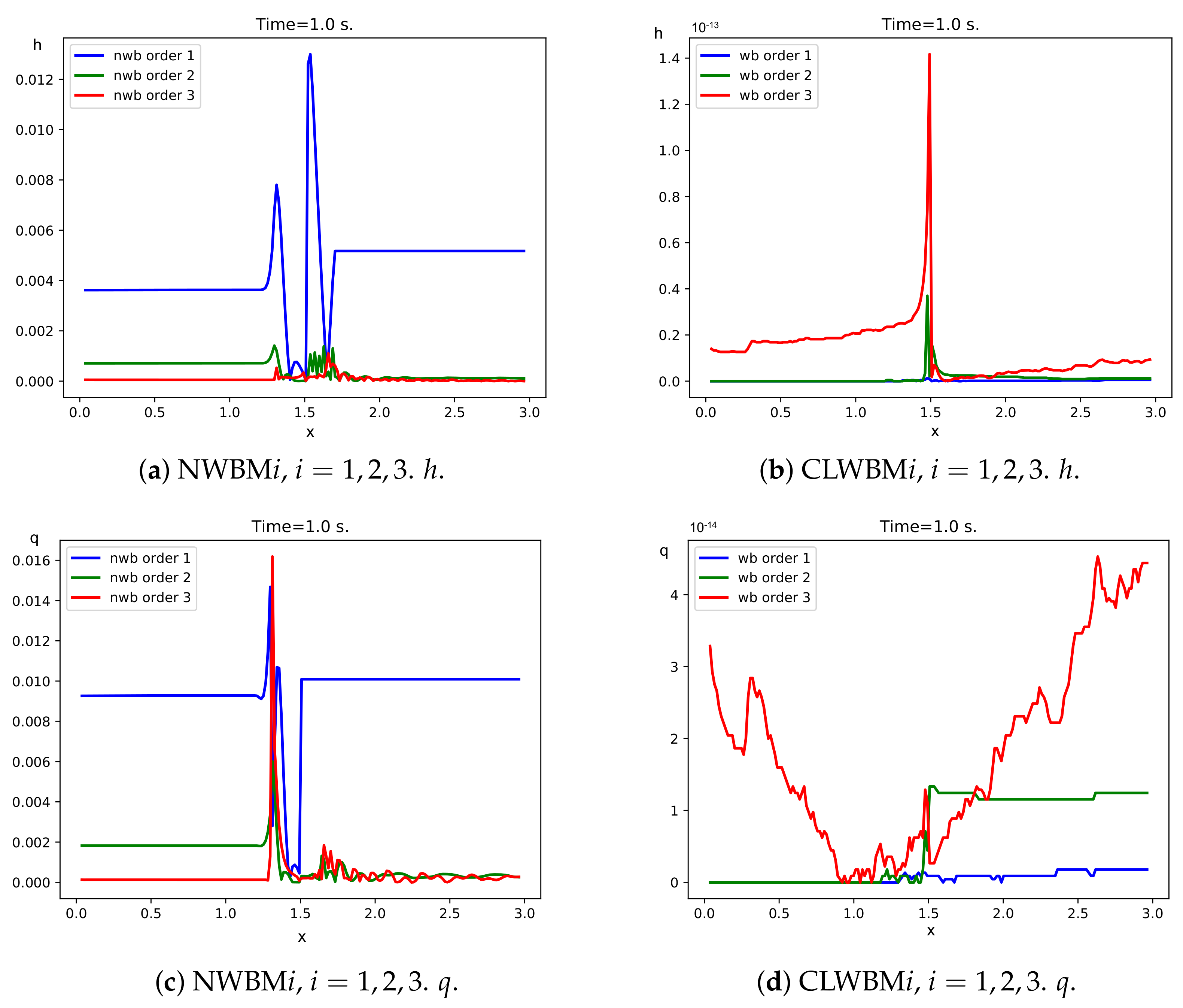
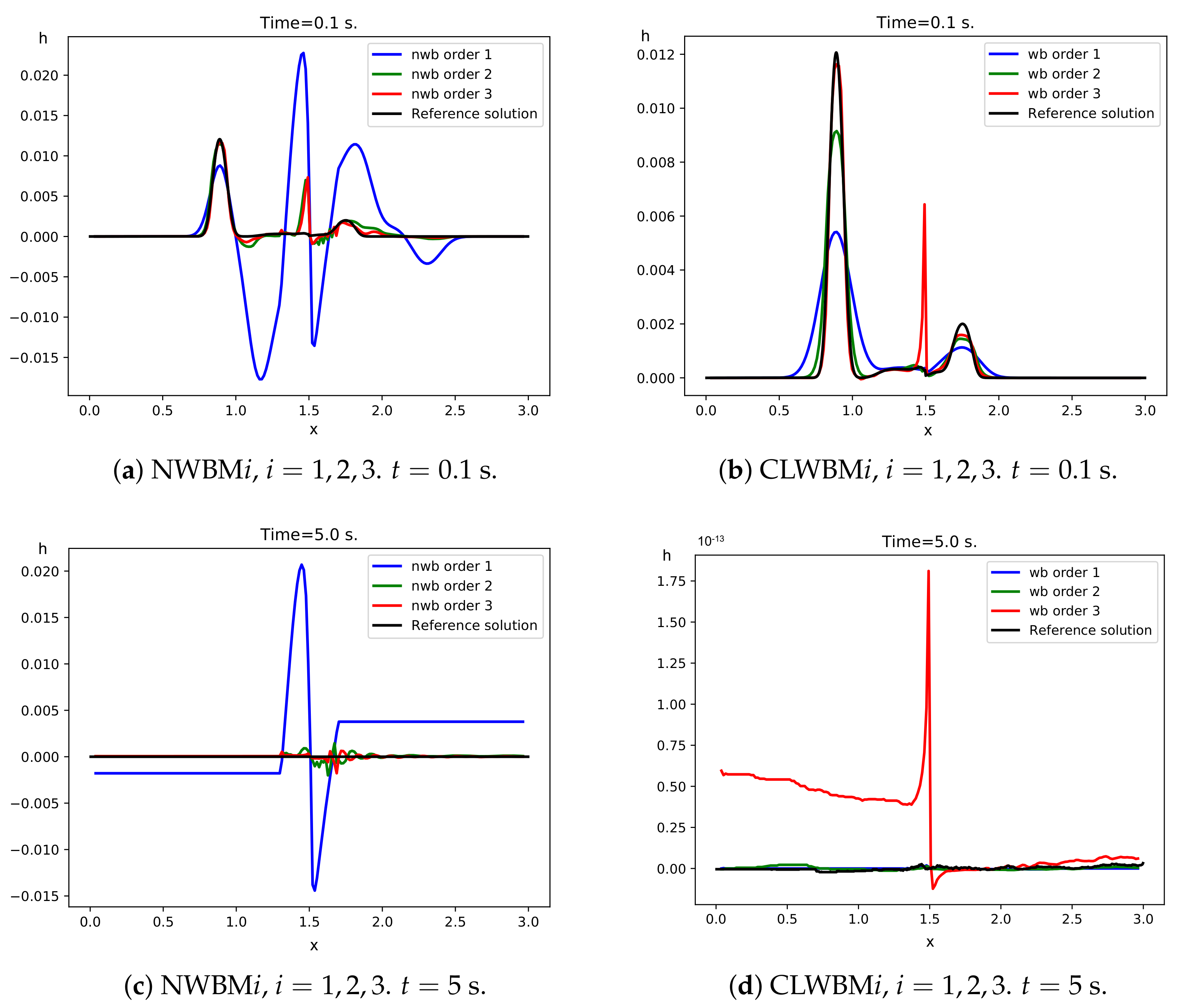
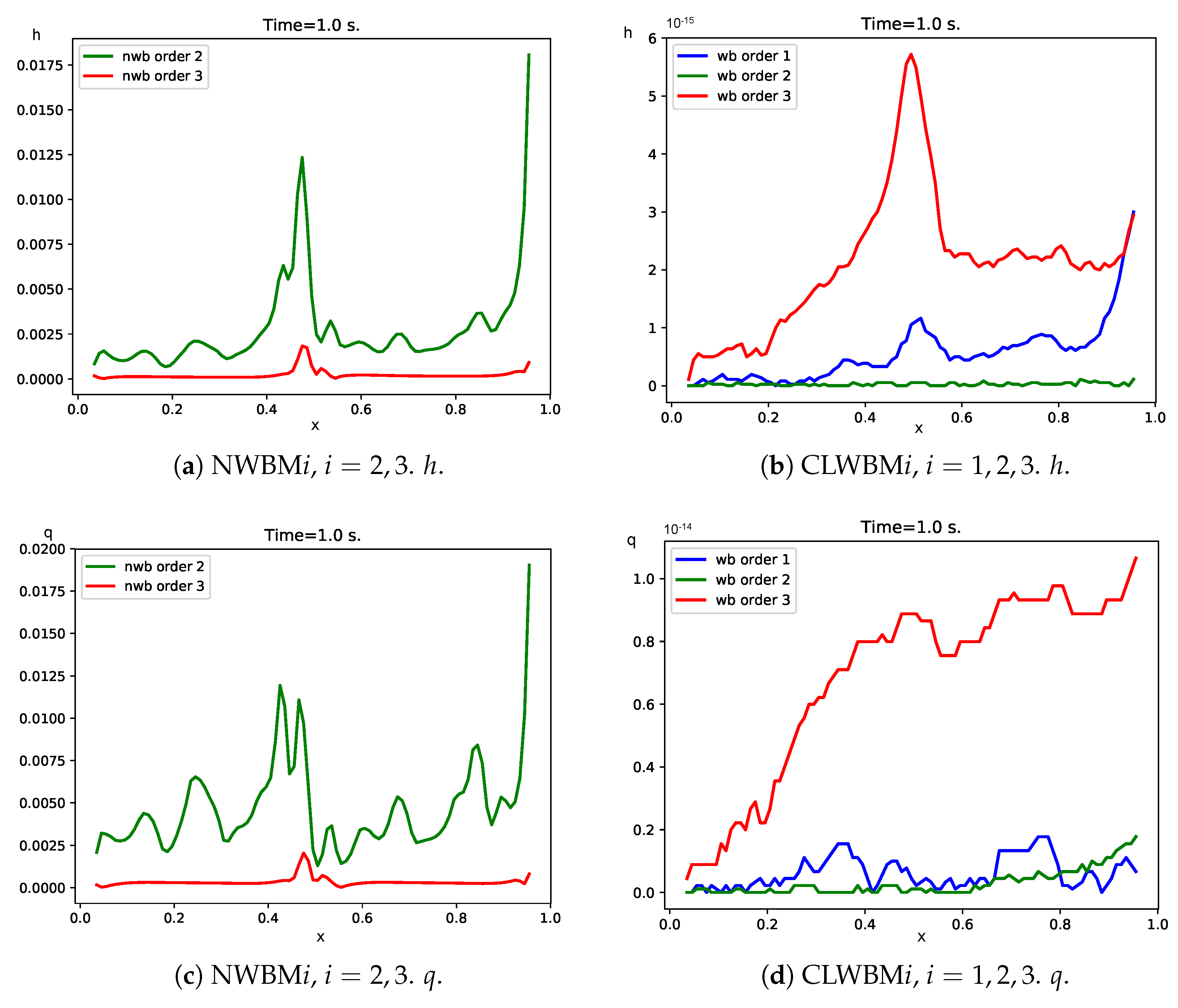
Figure 5.
Test 3.2. Reference and numerical solutions: differences with the stationary solution at times s for h with a 200-cell mesh.
Figure 5.
Test 3.2. Reference and numerical solutions: differences with the stationary solution at times s for h with a 200-cell mesh.
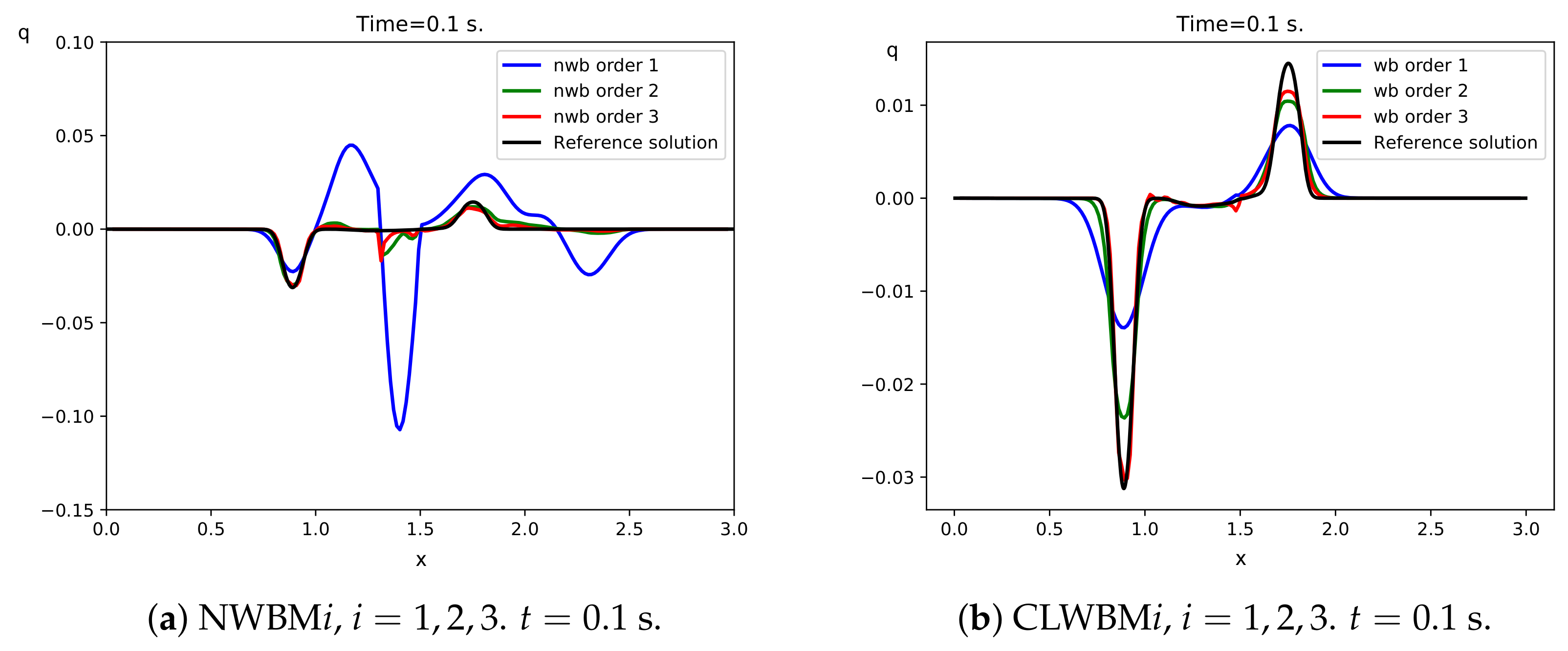
Figure 6.
Test 3.2. Reference and numerical solutions: differences with the stationary solution at times s for q for a 200-cell mesh.
Figure 6.
Test 3.2. Reference and numerical solutions: differences with the stationary solution at times s for q for a 200-cell mesh.
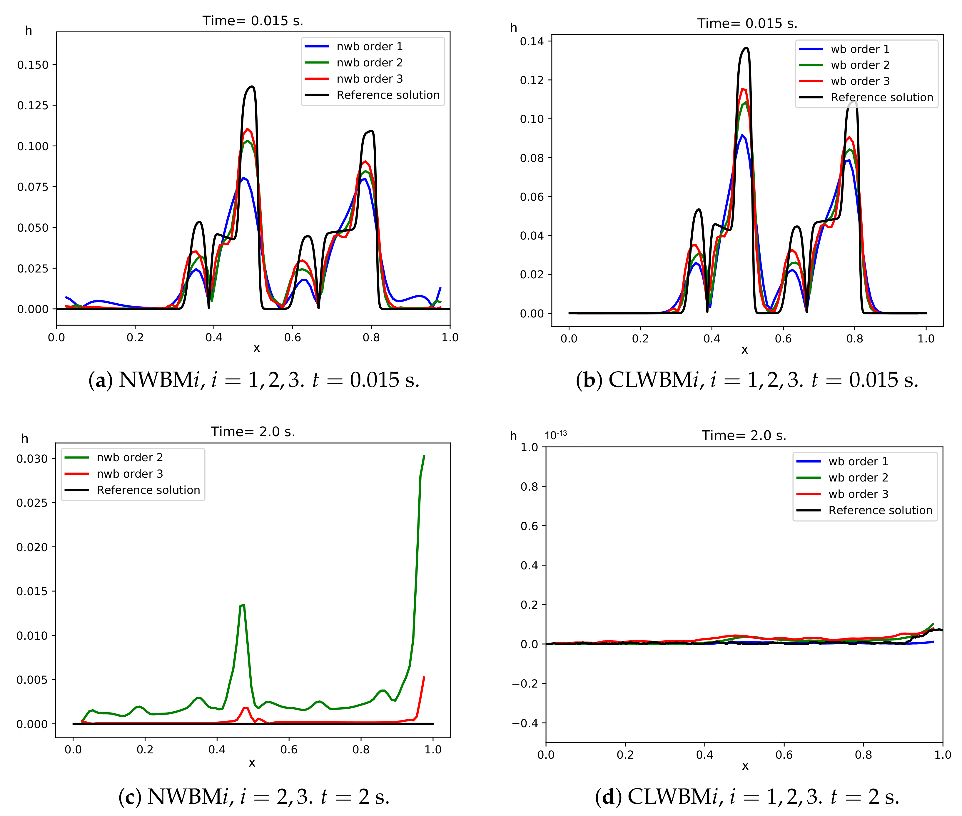
Figure 7.
Test 3.3. Reference and numerical solutions: differences with the stationary solution at times s and s for h for a 100-cell mesh.
Figure 7.
Test 3.3. Reference and numerical solutions: differences with the stationary solution at times s and s for h for a 100-cell mesh.
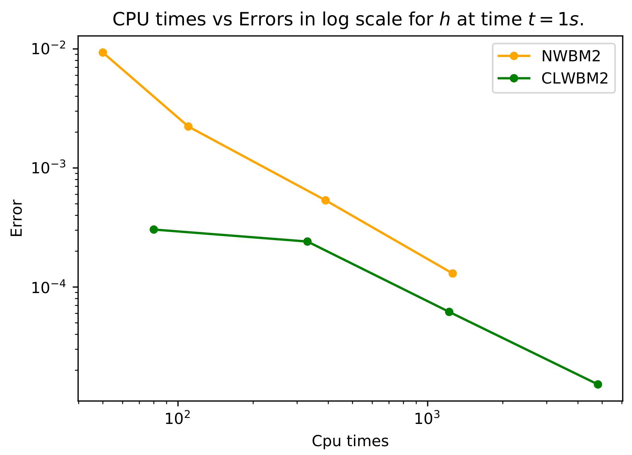
Figure 8.
Test 3.3. Errors in -norm with respect to the reference solution versus CPU times in milliseconds for the NWBM2 and CLWBM2 at time s.
Figure 8.
Test 3.3. Errors in -norm with respect to the reference solution versus CPU times in milliseconds for the NWBM2 and CLWBM2 at time s.
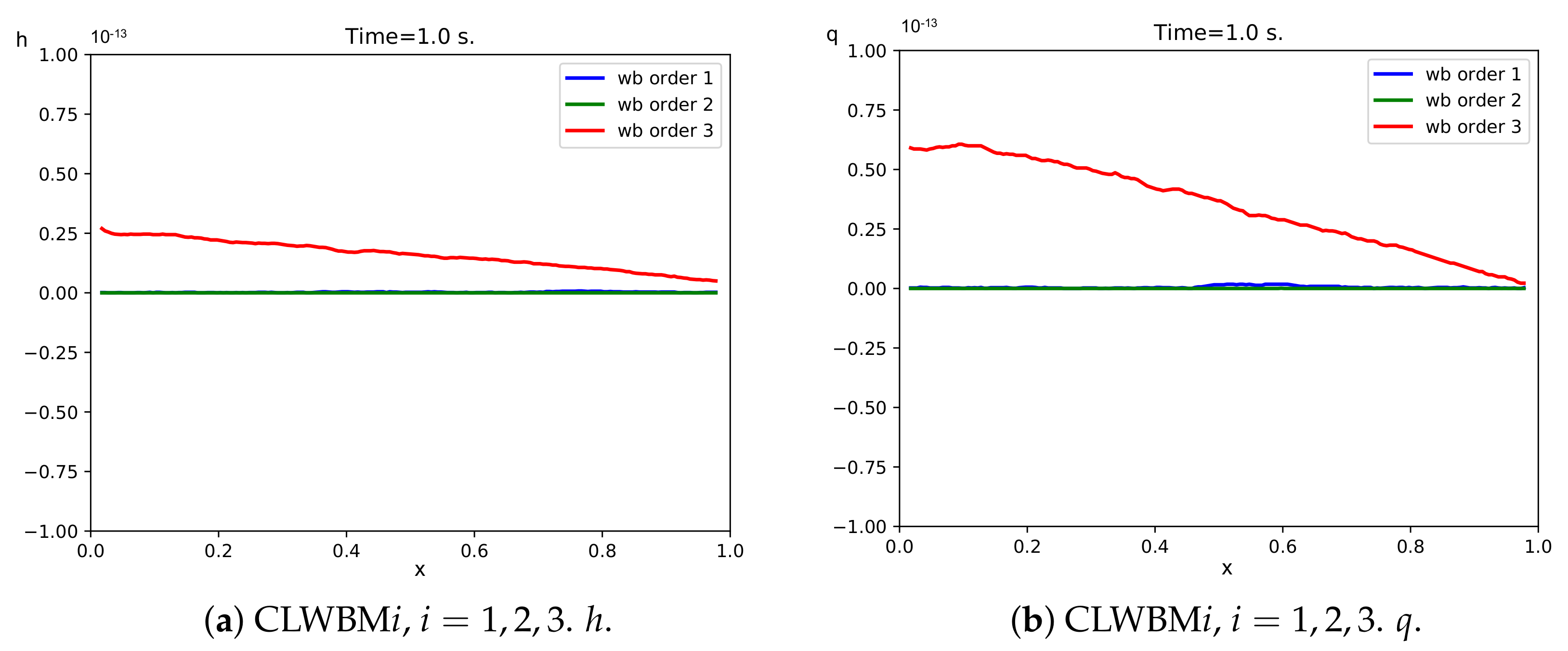
Figure 9.
Test 4.1. Differences between the stationary and the numerical solutions for CLWBMi, at time s for a 200-cell mesh.
Figure 9.
Test 4.1. Differences between the stationary and the numerical solutions for CLWBMi, at time s for a 200-cell mesh.
Figure 10.
Test 4.2. Reference and numerical solutions: differences with the stationary solution for CLWBMi, , at times s for h on a 100-cell mesh.
Figure 10.
Test 4.2. Reference and numerical solutions: differences with the stationary solution for CLWBMi, , at times s for h on a 100-cell mesh.
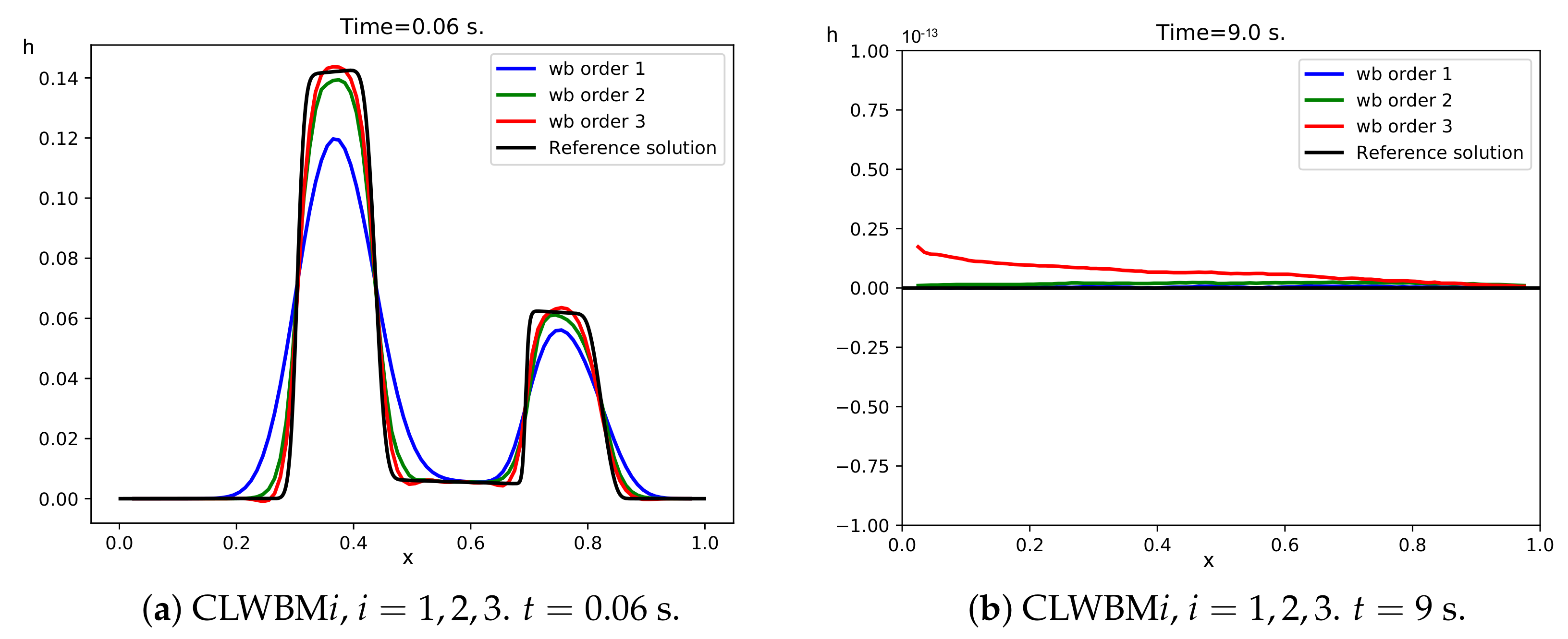
Figure 11.
Test 4.3. 100-cell numerical solutions and reference solution at time s.
Figure 11.
Test 4.3. 100-cell numerical solutions and reference solution at time s.
Figure 12.
Test 4.3. Differences between the stationary and the numerical solutions at time s with a 100-cell mesh.
Figure 12.
Test 4.3. Differences between the stationary and the numerical solutions at time s with a 100-cell mesh.
Figure 13.
Test 4.4. Reference and numerical solutions: differences with the stationary solution at times s for h, for a 100-cell mesh.
Figure 13.
Test 4.4. Reference and numerical solutions: differences with the stationary solution at times s for h, for a 100-cell mesh.
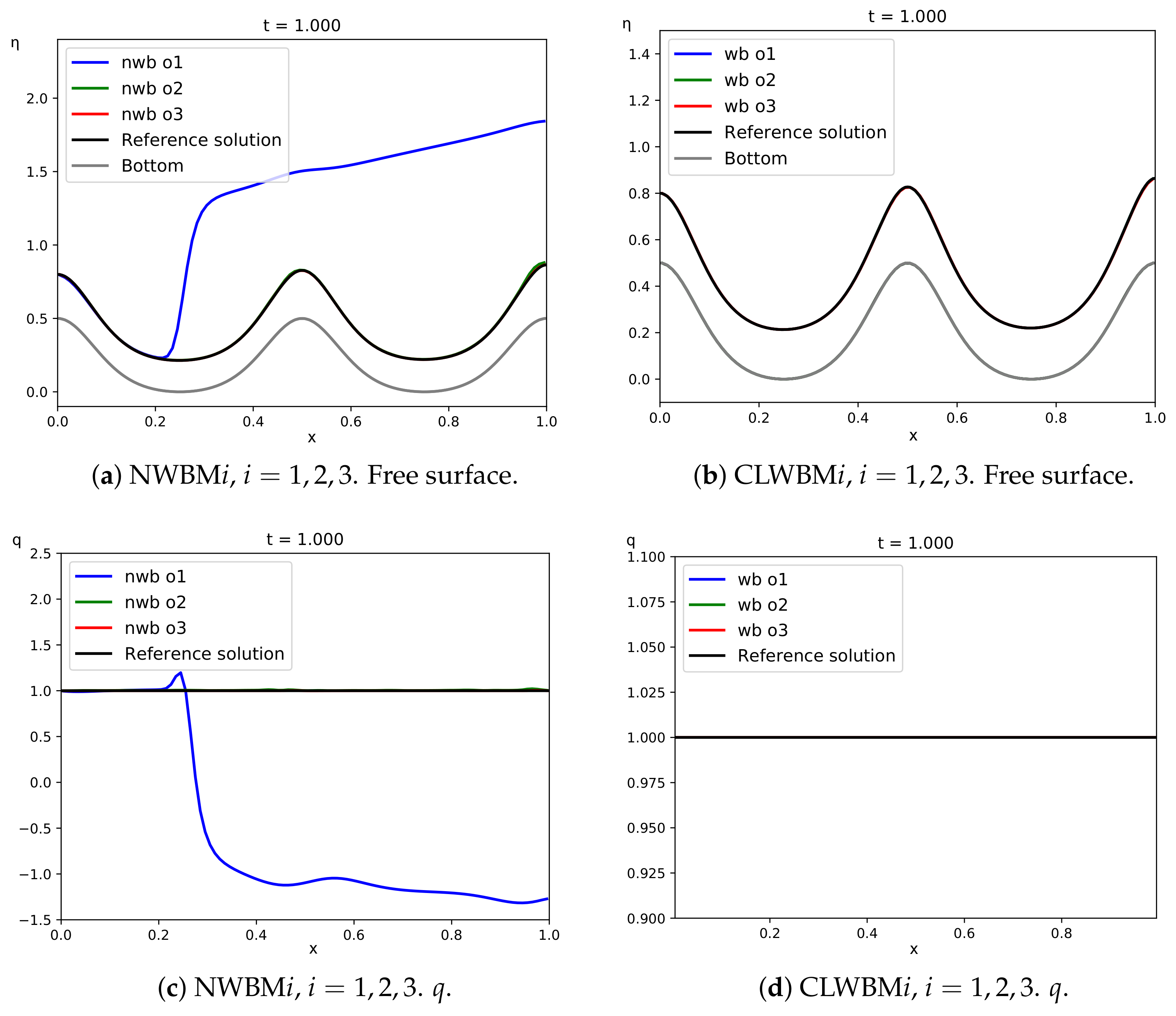
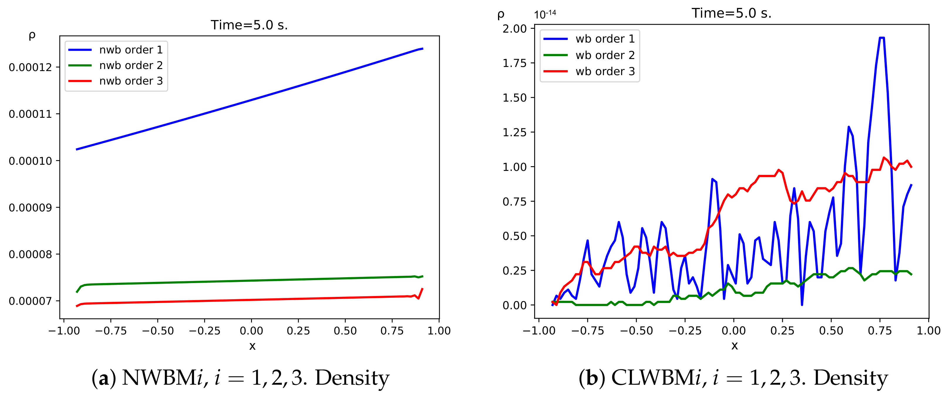
Figure 14.
Test 5.1. Differences between the stationary and the numerical solutions at time s for with a mesh of 100 cells.
Figure 14.
Test 5.1. Differences between the stationary and the numerical solutions at time s for with a mesh of 100 cells.
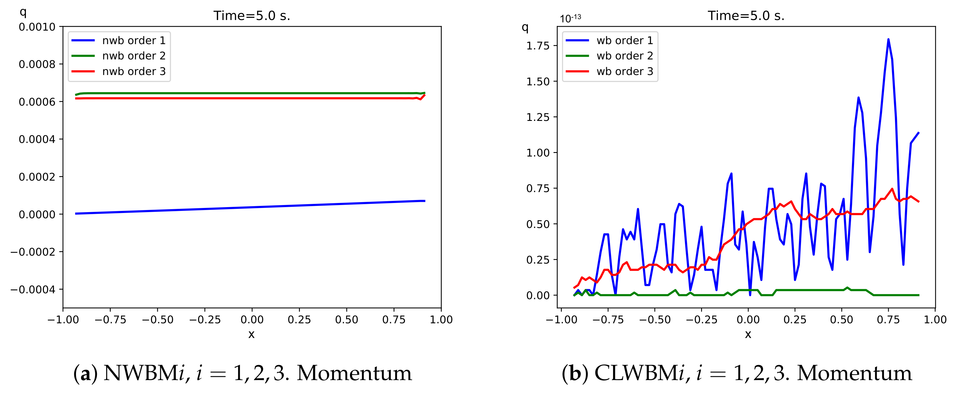
Figure 15.
Test 5.1. Differences between the stationary and the numerical solutions at time s for q with a mesh of 100 cells.
Figure 15.
Test 5.1. Differences between the stationary and the numerical solutions at time s for q with a mesh of 100 cells.
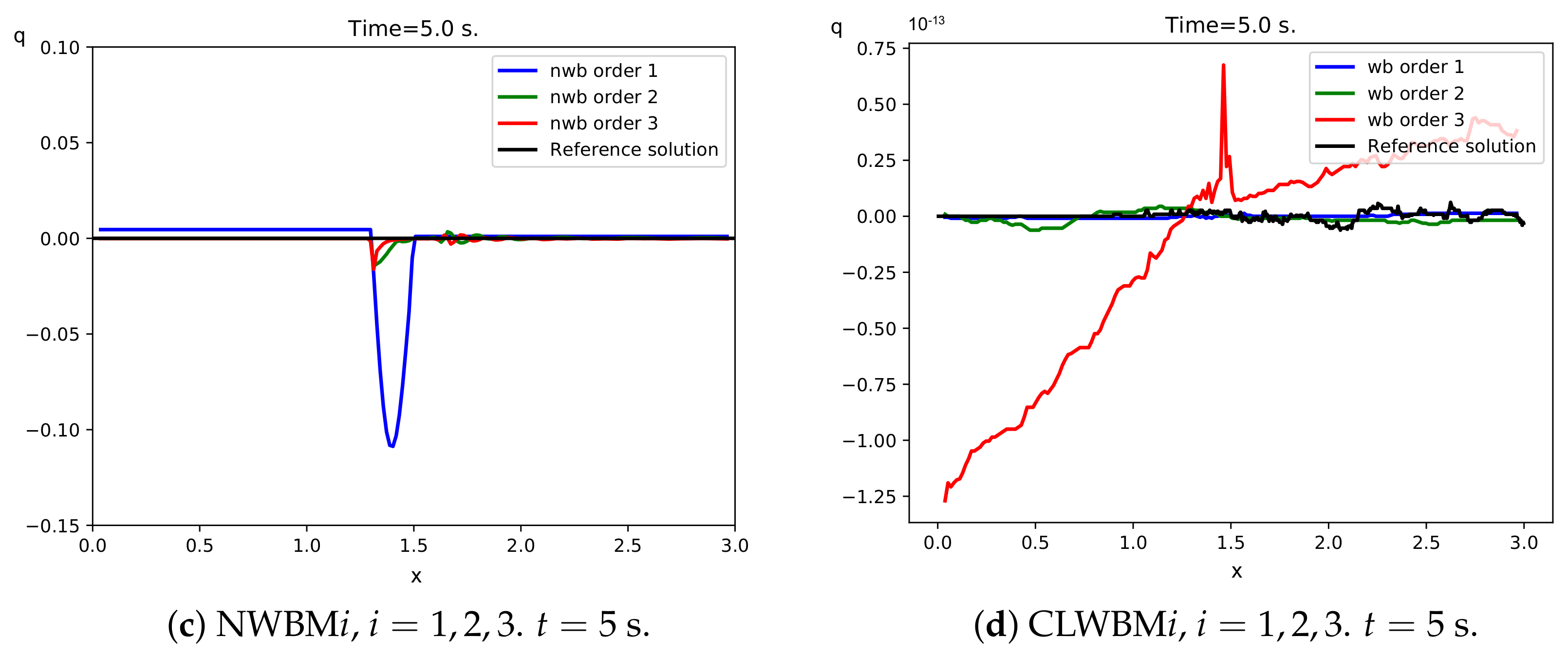
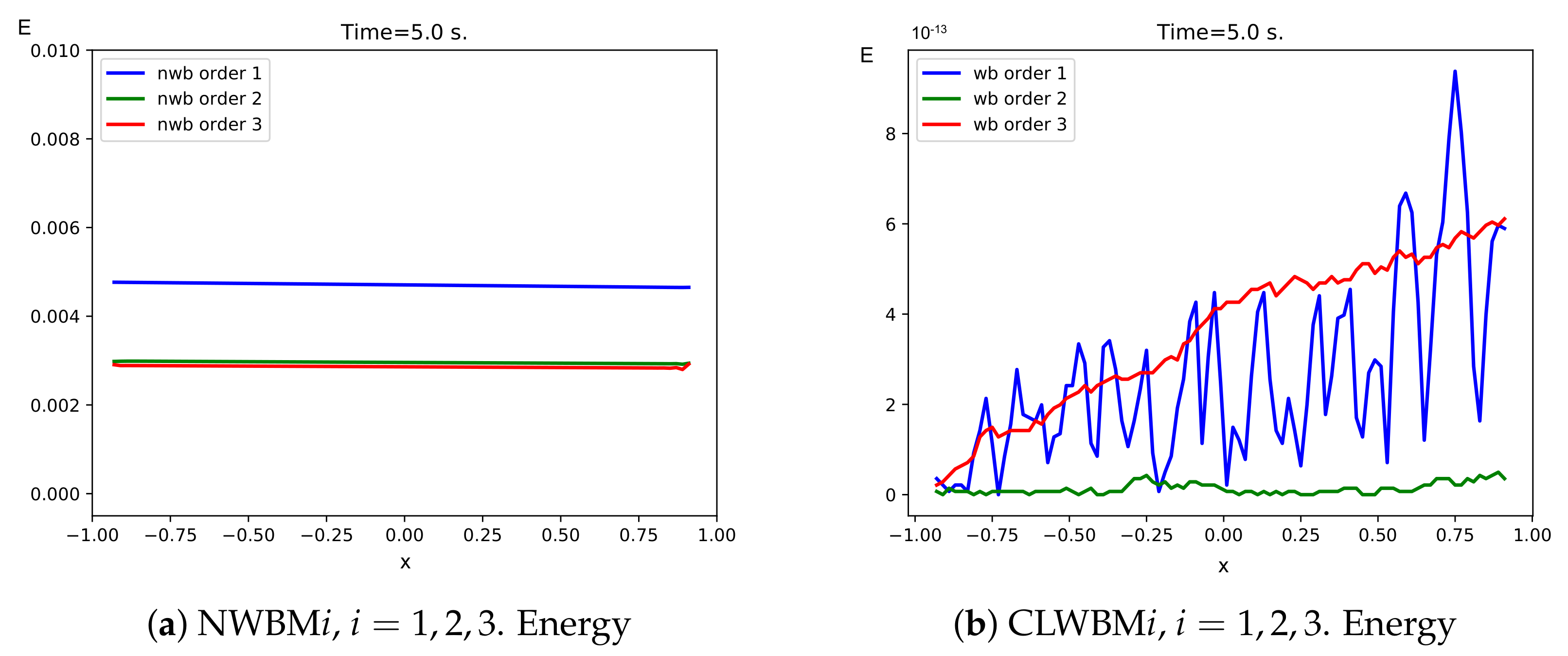
Figure 16.
Test 5.1. Differences between the stationary and the numerical solutions at time s for E with a mesh of 100 cells.
Figure 16.
Test 5.1. Differences between the stationary and the numerical solutions at time s for E with a mesh of 100 cells.
Table 1.
Test 1.1. errors at and convergence rates for CLWBM3 when option (a), (b), (c), and (d) are chosen to compute the initial cell averages.
Table 1.
Test 1.1. errors at and convergence rates for CLWBM3 when option (a), (b), (c), and (d) are chosen to compute the initial cell averages.
| Cells | Option (a) | Option (b) | Option (c) | Option (d) |
|---|
| Error | Order | Error | Order | Error | Order | Error | Order |
|---|
| 5 | 1.96 × | - | 1.82 × | - | 1.46 × | - | 4.88 × | - |
| 10 | 1.21 × | 4.015 | 1.12 × | 4.016 | 8.81 × | 4.054 | 7.44 × | - |
| 20 | 7.56 × | 4.003 | 7.01 × | 4.003 | 5.42 × | 4.023 | 3.00 × | - |
| 40 | 4.72 × | 4.001 | 4.38 × | 4.001 | 3.36 × | 4.011 | 7.94 × | - |
| 80 | 2.95 × | 4.000 | 2.74 × | 4.000 | 2.09 × | 4.006 | 9.00 × | - |
| 160 | 1.84 × | 4.000 | 1.71 × | 4.000 | 1.30 × | 4.003 | 1.23 × | - |
Table 2.
Test 1.1. Differences in -norm with respect to the stationary solution and convergence rates for NWBMi, .
Table 2.
Test 1.1. Differences in -norm with respect to the stationary solution and convergence rates for NWBMi, .
| Cells | NWBM1: Error | Order | NWBM2: Error | Order | NWBM3: Error | Order |
|---|
| 100 | 7.53 × | - | 2.44 × | - | 7.66 × | - |
| 200 | 3.78 × | 0.995 | 8.09 × | 1.591 | 9.62 × | 2.993 |
| 400 | 1.89 × | 1.002 | 2.16 × | 1.905 | 1.21 × | 2.995 |
| 800 | 9.43 × | 1.000 | 5.54 × | 1.963 | 1.51 × | 2.998 |
Table 3.
Test 1.1. Differences in -norm with respect to the stationary solution for WBMi, CWBMi, CLWBMi, .
Table 3.
Test 1.1. Differences in -norm with respect to the stationary solution for WBMi, CWBMi, CLWBMi, .
| Cells | Order 1: Error | Order 2: Error | Order 3: Error |
|---|
| WBM | CWBM | CLWBM | WBM | CWBM | CLWBM | WBM | CWBM | CLWBM |
|---|
| 100 | 4.21 × | 3.55 × | 2.50 × | 8.87 × | 3.63 × | 2.03 × | 3.20 × | 1.43 × | 8.17 × |
| 200 | 2.90 × | 5.54 × | 2.51 × | 4.42 × | 1.23 × | 1.66 × | 2.54 × | 2.43 × | 1.76 × |
| 400 | 1.84 × | 2.05 × | 1.12 × | 1.82 × | 3.64 × | 2.89 × | 7.40 × | 4.47 × | 4.45 × |
| 800 | 4.45 × | 2.67 × | 2.77 × | 1.83 × | 2.03 × | 2.05 × | 2.61 × | 9.48 × | 7.88 × |
Table 4.
Test 1.1. Computational times (milliseconds).
Table 4.
Test 1.1. Computational times (milliseconds).
| Cells | Order (i) | NWBMi | WBMi | CWBMi | CLWBMi |
|---|
| 1 | 20 | 30 | 70 | 30 |
| 100 | 2 | 30 | 60 | 140 | 110 |
| | 3 | 40 | 190 | 240 | 230 |
| 1 | 20 | 60 | 230 | 100 |
| 200 | 2 | 40 | 190 | 330 | 280 |
| | 3 | 110 | 480 | 530 | 520 |
| 1 | 50 | 180 | 520 | 220 |
| 400 | 2 | 100 | 530 | 1150 | 720 |
| | 3 | 350 | 1680 | 1980 | 1870 |
| 1 | 140 | 570 | 2020 | 870 |
| 800 | 2 | 270 | 2040 | 3580 | 2820 |
| | 3 | 1080 | 5540 | 6600 | 5960 |
Table 5.
Test 2.1. Differences in -norm with respect to the stationary solution and convergence rates for NWBMi, .
Table 5.
Test 2.1. Differences in -norm with respect to the stationary solution and convergence rates for NWBMi, .
| Cells | Error () | Order | Error () | Order | Error () | Order |
|---|
| 100 | 2.72 × | - | 1.43 × | - | 2.53 × | - |
| 200 | 1.34 × | 1.021 | 2.43 × | 5.879 | 1.74 × | 10.503 |
| 400 | 6.58 × | 1.026 | 8.19 × | 1.569 | 1.14 × | 7.250 |
| 800 | 3.24 × | 1.022 | 2.34 × | 1.806 | 1.41 × | 3.016 |
Table 6.
Test 2.1. Differences in -norm with respect to the stationary solution for CWBMi, CLWBMi, .
Table 6.
Test 2.1. Differences in -norm with respect to the stationary solution for CWBMi, CLWBMi, .
| Cells | Order 1: Error | Order 2: Error | Order 3: Error |
|---|
| CWBM | CLWBM | CWBM | CLWBM | CWBM | CLWBM |
|---|
| 100 | 9.71 × | 3.00 × | 1.76 × | 6.39 × | 1.99 × | 8.50 × |
| 200 | 7.56 × | 5.37 × | 3.46 × | 5.15 × | 2.97 × | 2.51 × |
| 400 | 4.00 × | 5.68 × | 7.53 × | 5.73 × | 3.31 × | 4.85 × |
| 800 | 5.97 × | 4.63 × | 8.54 × | 5.31 × | 6.63 × | 9.61 × |
Table 7.
Test 2.1. Computational cost (milliseconds). s.
Table 7.
Test 2.1. Computational cost (milliseconds). s.
| Cells | Order(i) | NWBMi | CWBMi | CLWBMi |
|---|
| 1 | 10 | 340 | 130 |
| 100 | 2 | 20 | 690 | 280 |
| | 3 | 40 | 1390 | 490 |
| 1 | 30 | 1280 | 230 |
| 200 | 2 | 60 | 2350 | 440 |
| | 3 | 180 | 5190 | 1230 |
Table 8.
Test 2.2. Differences in -norm with respect to the stationary solution for NWBMi, CWBMi, and CLWBMi () at time s.
Table 8.
Test 2.2. Differences in -norm with respect to the stationary solution for NWBMi, CWBMi, and CLWBMi () at time s.
| Method | Error () | Error () | Error () |
|---|
| NWBMi | 2.43 × | 1.71 × | 1.05 × |
| CWBMi | 1.09 × | 4.47 × | 3.34 × |
| CLWBMi | 2.52 × | 1.19 × | 1.24 × |
Table 9.
Test 3.1. Differences in -norm with respect to the stationary solution and convergence rates for NWBMi, .
Table 9.
Test 3.1. Differences in -norm with respect to the stationary solution and convergence rates for NWBMi, .
| Cells | Error () | Order | Error () | Order | Error () | Order |
|---|
| | | | |
| 100 | 4.99 × | - | 7.63 × | - | 5.99 × | - |
| 200 | 1.31 × | 1.923 | 1.27 × | 2.583 | 8.86 × | 2.757 |
| 400 | 3.87 × | 1.766 | 1.84 × | 2.790 | 6.20 × | 3.838 |
| 800 | 1.56 × | 1.314 | 5.31 × | 1.794 | 6.88 × | 3.172 |
| Cells | Error () | Order | Error () | Order | Error () | Order |
| | | | |
| 100 | 1.28 × | - | 1.89 × | - | 1.72 × | - |
| 200 | 2.81 × | 2.188 | 3.18 × | 2.575 | 2.35 × | 2.866 |
| 400 | 9.29 × | 1.161 | 4.81 × | 2.724 | 2.09 × | 3.489 |
| 800 | 4.09 × | 1.168 | 1.37 × | 1.812 | 2.29 × | 3.190 |
Table 10.
Test 3.1. Differences in -norm with respect to the stationary solution for CLWBMi, .
Table 10.
Test 3.1. Differences in -norm with respect to the stationary solution for CLWBMi, .
| Cells | Error (i = 1) | Error (i = 2) | Error (i = 3) |
|---|
| | | | | | | |
| 100 | 1.46 × | 2.13 × | 2.80 × | 1.44 × | 2.88 × | 3.63 × |
| 200 | 4.95 × | 3.00 × | 3.03 × | 1.44 × | 3.94 × | 5.53 × |
| 400 | 2.94 × | 1.74 × | 4.75 × | 1.20 × | 8.89 × | 1.45 × |
| 800 | 1.50 × | 6.92 × | 3.25 × | 1.21 × | 1.04 × | 1.55 × |
Table 11.
Test 3.1. Computational cost (milliseconds). s.
Table 11.
Test 3.1. Computational cost (milliseconds). s.
| Cells | Order (i) | NWBMi | CLWBMi |
|---|
| 1 | 20 | 30 |
| 100 | 2 | 30 | 130 |
| | 3 | 70 | 320 |
| 1 | 30 | 60 |
| 200 | 2 | 80 | 370 |
| | 3 | 200 | 1100 |
Table 12.
Test 3.2. Differences in -norm for NWBMi and CLWBMi () with respect to the stationary solution using a 200-cell mesh at time s.
Table 12.
Test 3.2. Differences in -norm for NWBMi and CLWBMi () with respect to the stationary solution using a 200-cell mesh at time s.
| Method | Error () | Error () | Error () |
|---|
| | | | | | | |
| NWBMi | 1.01 × | 2.13 × | 4.83 × | 2.00 × | 2.70 × | 1.30 × |
| CLWBMi | 5.11 × | 4.32 × | 1.95 × | 6.47 × | 7.89 × | 1.38 × |
Table 13.
Test 3.3. Differences in -norm for NWBMi and CLWBMi () with respect to the stationary solution for the 100-cell mesh at time s.
Table 13.
Test 3.3. Differences in -norm for NWBMi and CLWBMi () with respect to the stationary solution for the 100-cell mesh at time s.
| Method | Error () | Error () | Error () |
|---|
| | | | | | | |
| NWBMi | 5.08 × | 1.94 × | 9.33 × | 3.51 × | 6.02 × | 2.12 × |
| CLWBMi | 1.81 × | 5.54 × | 1.95 × | 4.45 × | 2.46 × | 5.20 × |
Table 14.
Test 4.1. Differences in -norm with respect to the stationary solution for CLWBMi () for the 200-cell mesh at time s.
Table 14.
Test 4.1. Differences in -norm with respect to the stationary solution for CLWBMi () for the 200-cell mesh at time s.
| Method | Error () | Error () | Error () |
|---|
| | | | | | | |
| CLWBMi | 2.24 × | 5.06 × | 0.00 | 5.56 × | 1.58 × | 3.38 × |
Table 15.
Test 4.2. Differences in -norm with respect to the stationary solution for CLWBMi () for the 100-cell mesh at time s.
Table 15.
Test 4.2. Differences in -norm with respect to the stationary solution for CLWBMi () for the 100-cell mesh at time s.
| Method | Error () | Error () | Error () |
|---|
| | | | | | | |
| CLWBMi | 2.99 × | 3.97 × | 1.81 × | 2.76 × | 6.50 × | 1.77 × |
Table 16.
Test 4.3. Differences in -norm with respect to the stationary solution for NWBMi and CLWBMi () for the 100-cell mesh at time s.
Table 16.
Test 4.3. Differences in -norm with respect to the stationary solution for NWBMi and CLWBMi () for the 100-cell mesh at time s.
| Method | Error () | Error () | Error () |
|---|
| | | | | | | |
| NWBMi | 8.28 × | 1.54 | 3.61 × | 4.88 × | 3.65 × | 4.30 × |
| CLWBMi | 7.03 × | 5.85 × | 3.22 × | 3.75 × | 2.14 × | 6.87 × |
Table 17.
Test 4.4. Differences in -norm with respect to the stationary solution for NWBMi and CLWBMi () at time s for a 100-cell mesh.
Table 17.
Test 4.4. Differences in -norm with respect to the stationary solution for NWBMi and CLWBMi () at time s for a 100-cell mesh.
| Method | Error () | Error () | Error () |
|---|
| | | | | | | |
| NWBMi | 2.42 | 6.12 | 3.57 × | 4.87 × | 1.39 × | 4.30 × |
| CLWBMi | 3.73 × | 3.60 × | 1.80 × | 1.99 × | 2.64 × | 8.93 × |
Table 18.
Test 5.1. Differences in -norm with respect to the stationary solution for NWBMi and CLWBMi () for the mesh with 100 cells at time s.
Table 18.
Test 5.1. Differences in -norm with respect to the stationary solution for NWBMi and CLWBMi () for the mesh with 100 cells at time s.
| Method | Error () | Error () | Error () |
|---|
| h |
| NWBMi | 2.23 × | 9.41 × | 9.51 × |
| CLWBMi | 6.97 × | 6.58 × | 3.20 × |
| q |
| NWBMi | 1.45 × | 1.28 × | 5.95 × |
| CLWBMi | 2.22 × | 2.81 × | 2.77 × |
| E |
| NWBMi | 1.38 × | 1.22 × | 5.78 × |
| CLWBMi | 1.24 × | 8.13 × | 7.15 × |
Table 19.
Test 5.1. Computational cost (milliseconds) for the mesh with 100 cells. s.
Table 19.
Test 5.1. Computational cost (milliseconds) for the mesh with 100 cells. s.
| Order (i) | NWBMi | CWBMi | CLWBMi |
|---|
| 1 | 120 | 4480 | 220 |
| 2 | 250 | 8960 | 1440 |
| 3 | 670 | 19430 | 4750 |


