
Rough Set Approach for Identifying the Combined Effects of Heat and Mass Transfer Due to MHD Nanofluid Flow over a Vertical Rotating Frame


Abstract
:1. Introduction
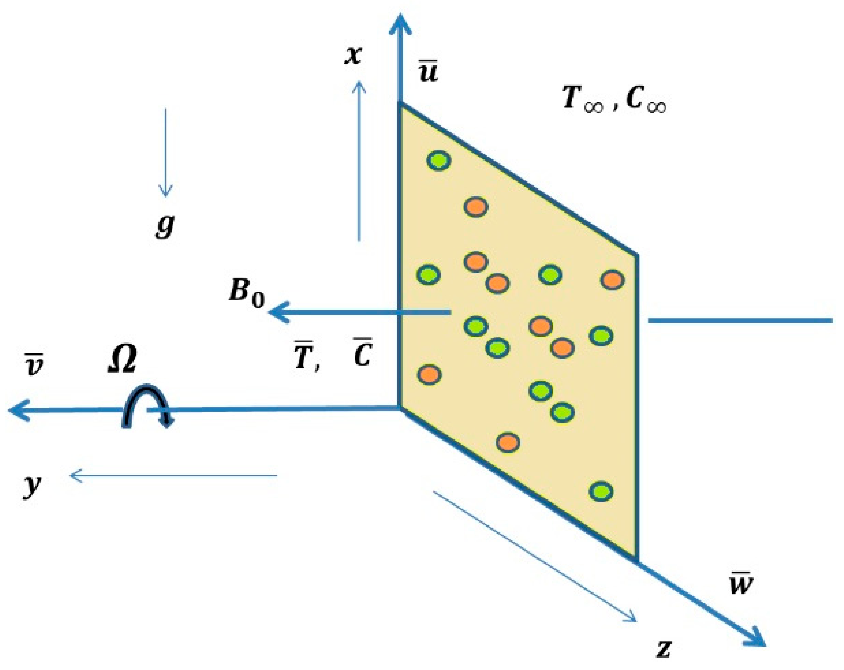
2. The Mathematical Framework
- Consider the physical quantities depend only on y.
- A magnetic field of constant strength is introduced in a direction parallel to y-axis in the direction of the fluid flow.
- The system spins about the normal axis with an angular velocity .
- assume that there exists a homogenous chemical reaction of first-order with rate constant between the diffusing species and the fluid.
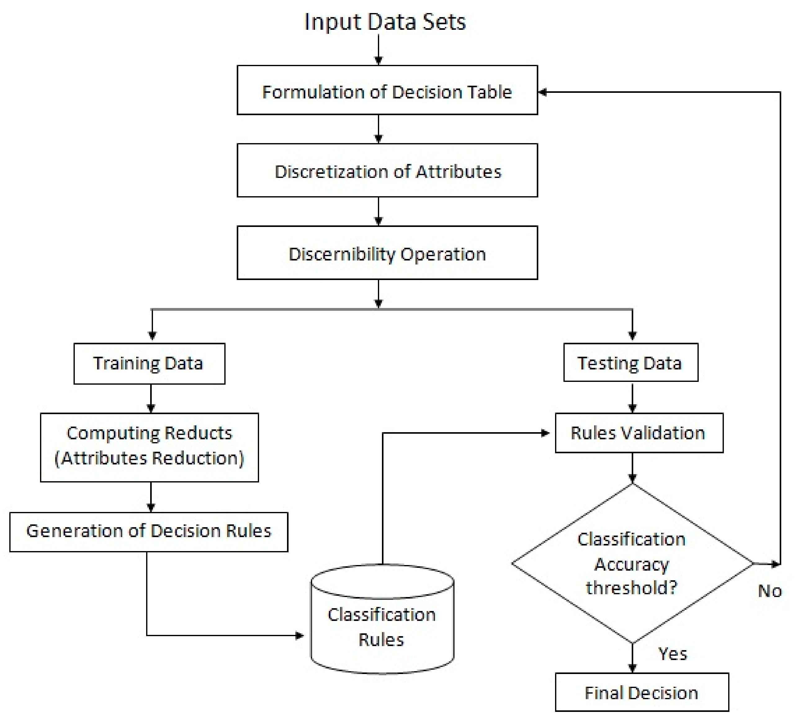
- Formulation of the Decision table
- Discretization of attributes
- Reduction of attributes
- Extracting the Decision Rules
3. Results and Discussion
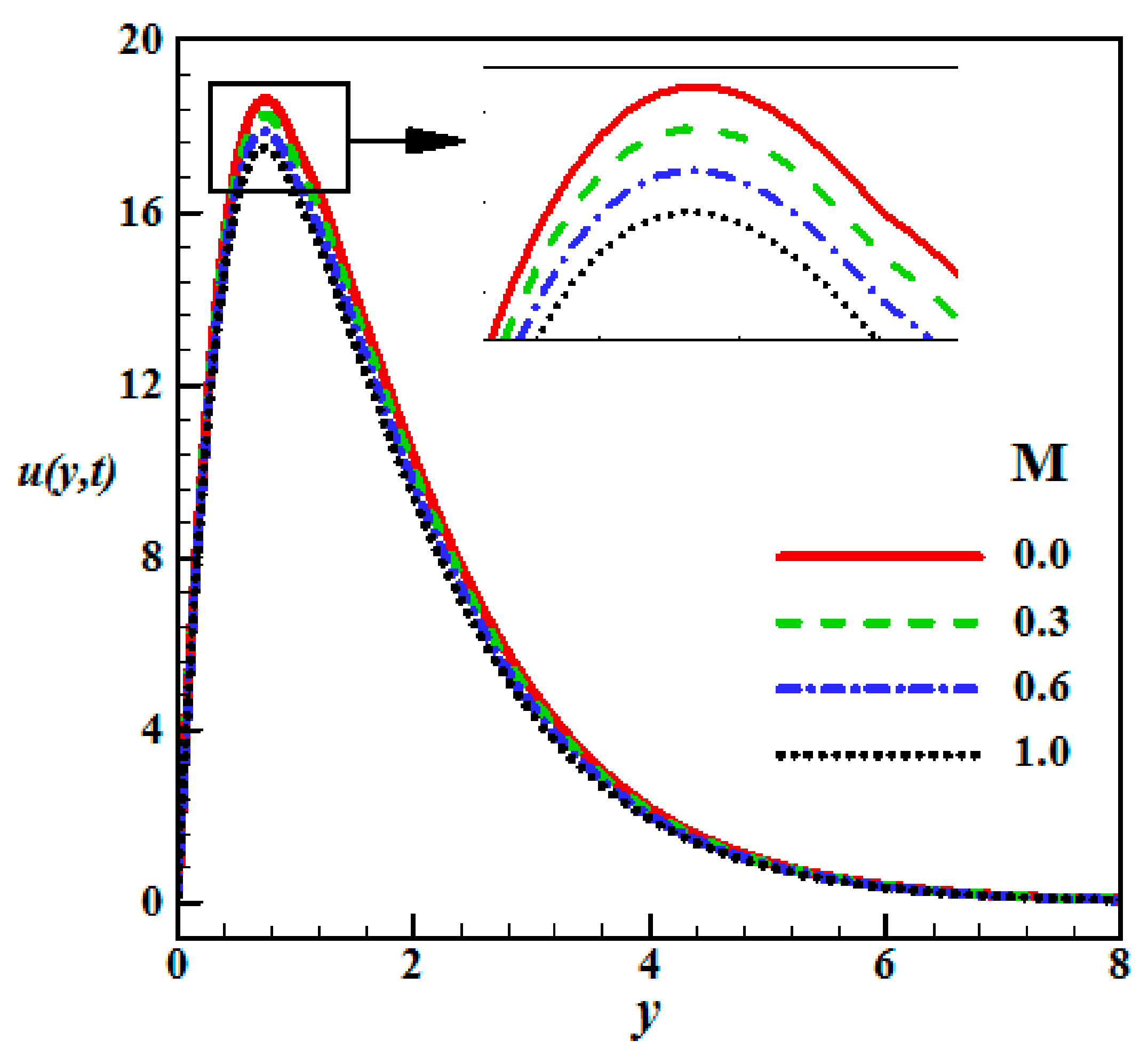
- Figure 6 shows the impact of the magnetic field parameter on the dimensionless velocity . It is noticed that increasing values of leads to deceleration of the dimensionless velocity . The physical explanation of this issue is that as the magnetic field is applied; a resistance force opposing the fluid motion is generated, therefore causing a decrease in the velocity of the liquid.
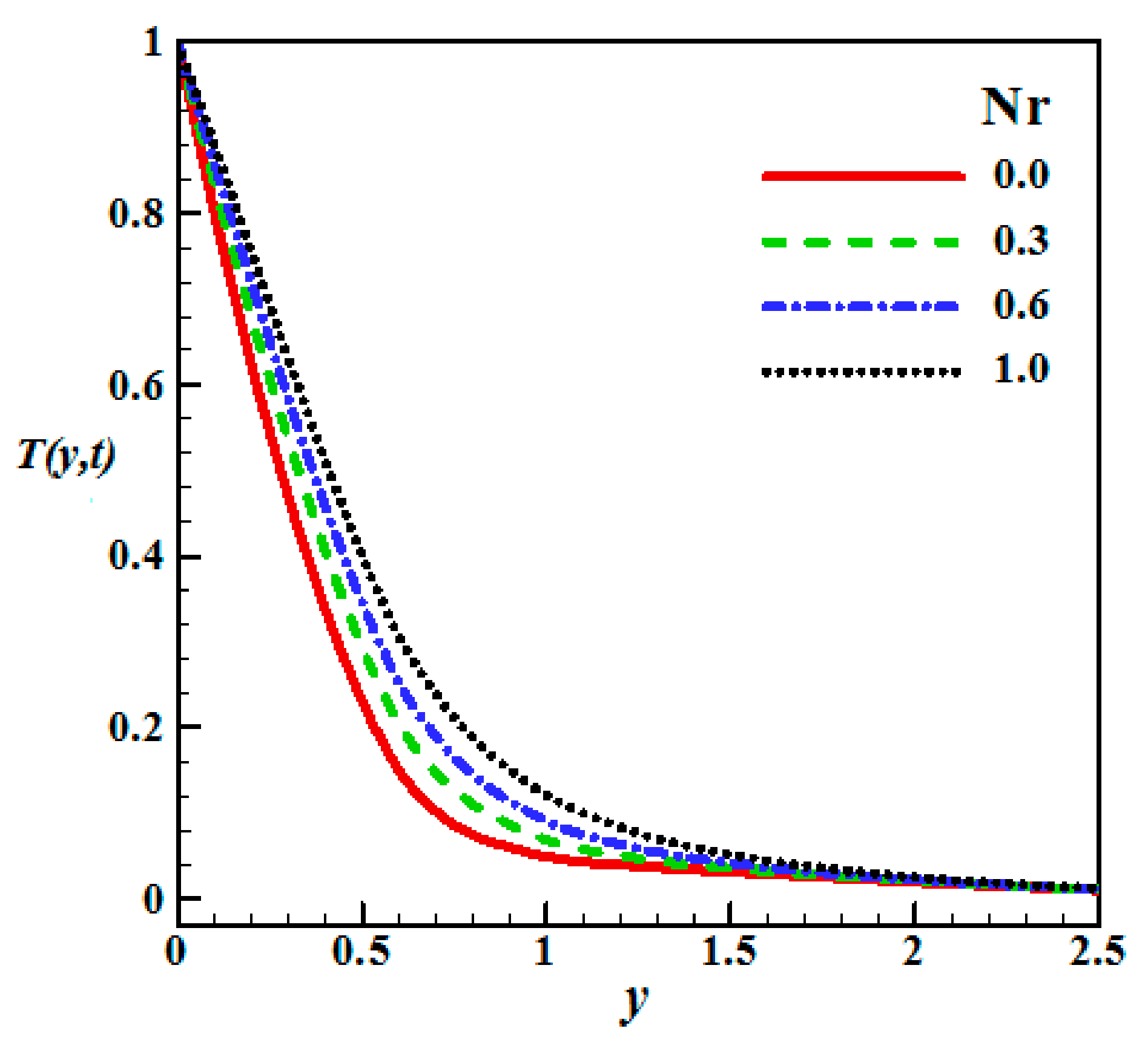
- Figure 7 displays the influence of the radiation parameter Nr on the dimensionless temperature, where an enhancement in the temperature profile occurred at all the points in the presence of thermal radiation. The physical explanation of this issue is that bigger estimations of Nr generate more heat into the fluid leading to a rise in the temperature.
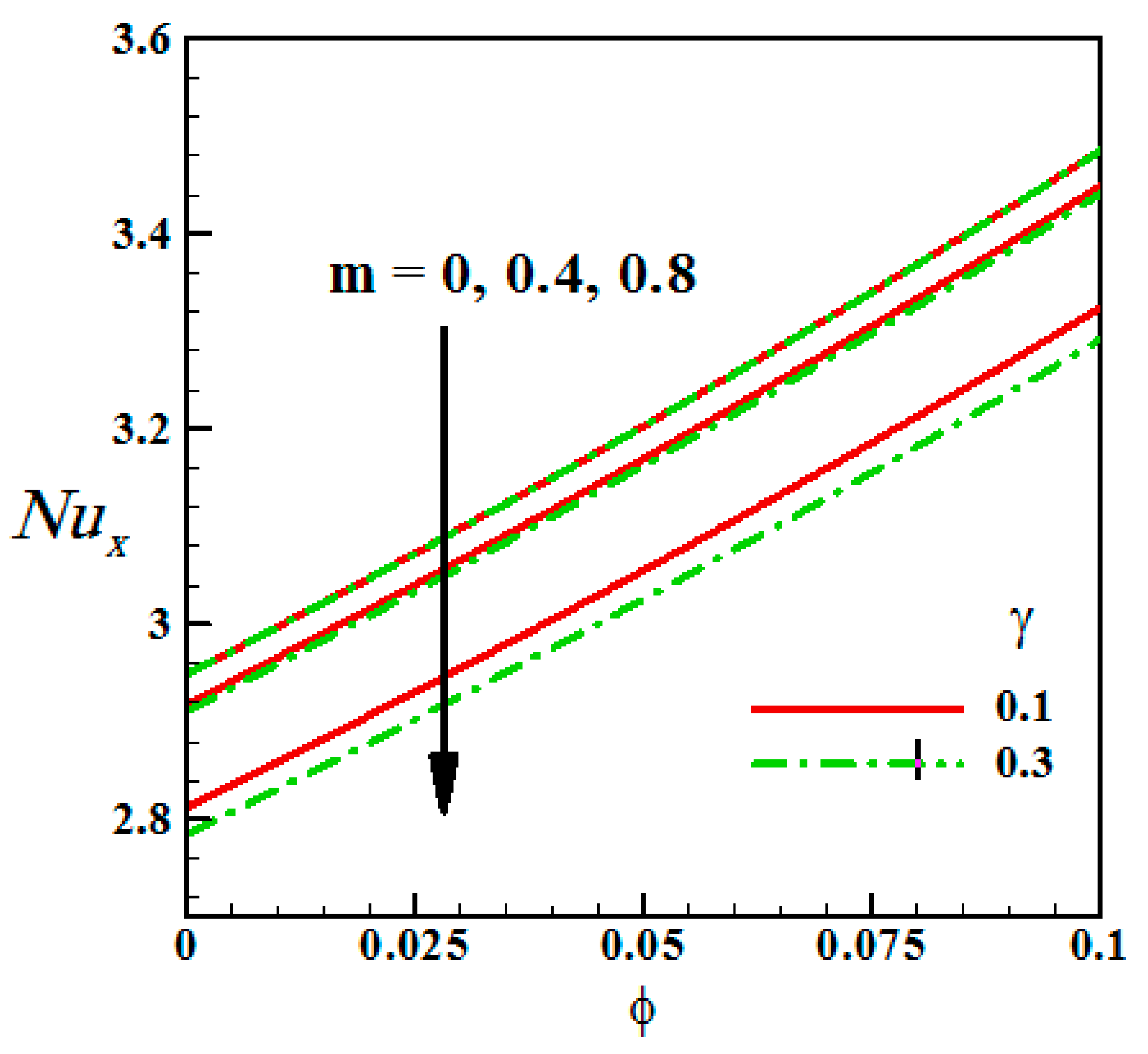
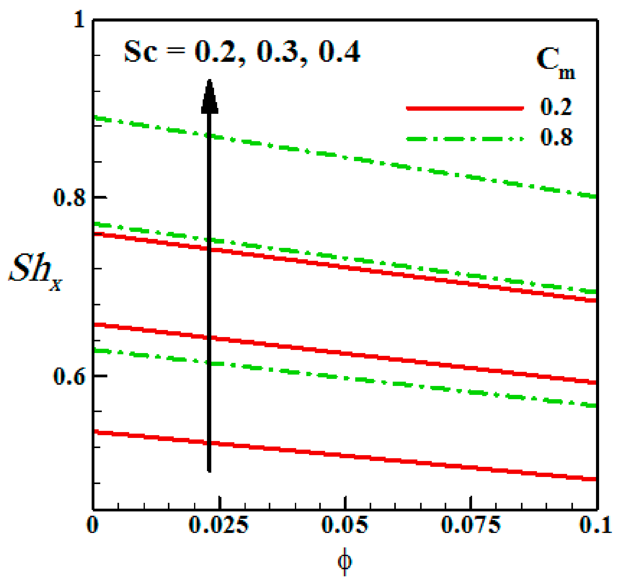
- The chemical reaction parameter decreases the heat transfer coefficient but increases the mass transfer rate. Increase in the values of implies more interaction of species concentration with the momentum boundary layer and less interaction with thermal boundary layer. Hence, chemical reaction parameter has more significant effect on Sherwood number than it does on Nusselt number.
- It can only deal with discrete databases. However, in the real-life applications databases are numerical; therefore, the continuous data need to be discretized before attribute reduction by using one of the following methods: discretization based on information entropy, box method for equal frequency, discretization based on cluster analysis. The discretization process leads to information loss. Therefore, it is desirable to develop an efficient method which can deal with numerical databases directly.
- It depends upon the principles of equivalence relations. however, in real life applications equivalence relations are relatively not suitable; so, it is required to find a way to make the relations less significant by removing one or more of the three requirements of an equivalence relation.
4. Conclusions
- This research clarifies that the proposed rule induction approach based on rough sets theory is a unique and viable posterior classification approach to extract knowledge
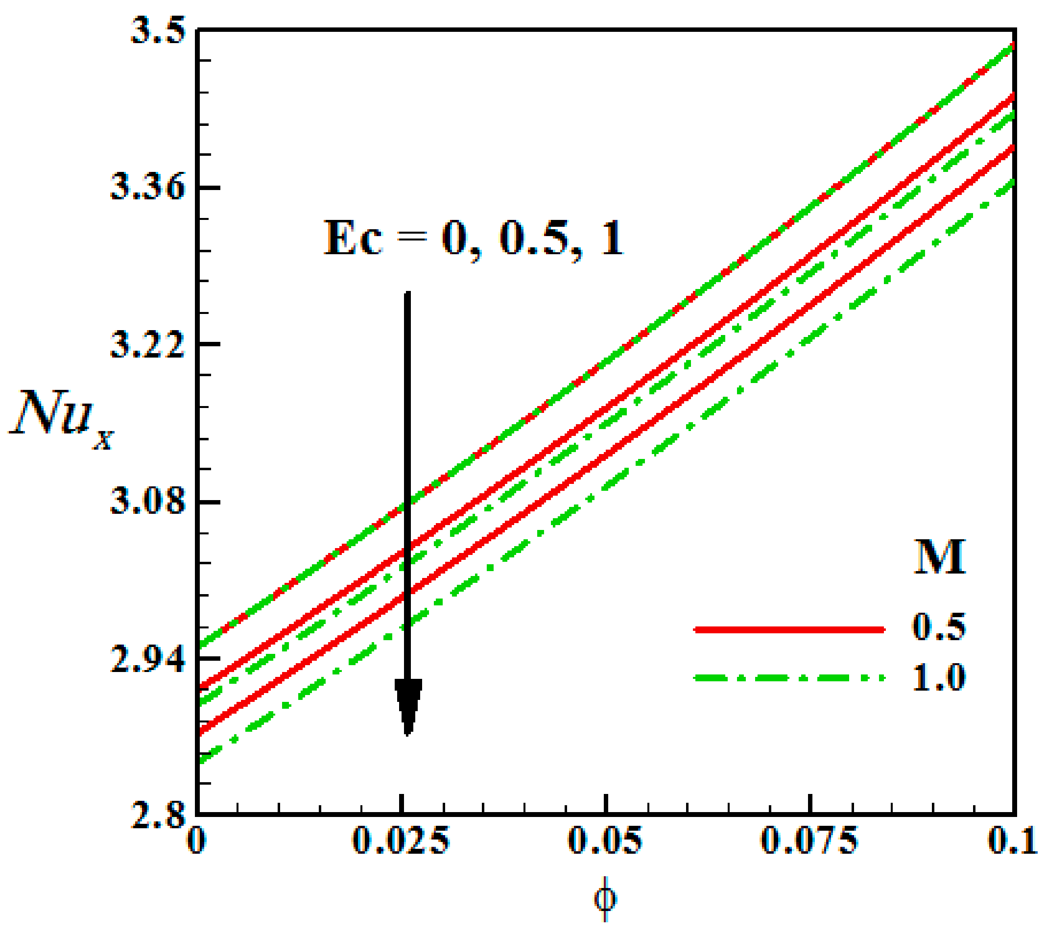
- The local Nusselt number increases with an increase in the volume fraction of nanoparticles and the radiation parameter.
- An increase in magnetic parameter, Brinkman parameter and Eckert number reduce the local Nusselt number.
- With a rise in the concentration gradient, mass transport increases to increase the value of .
- Higher values of the magnetic field parameter cause decrease in the velocity of the liquid and gradual drop in the secondary velocity w(y, t) is noticed.
- The chemical reaction parameter decreases the heat transfer coefficient but increases the mass transfer rate.
- The chemical reaction parameter has more significant effect on Sherwood number than it does on Nusselt number.
- As the radiation parameter (Nr) increases more heat is produced into the fluid and consequently increases the temperature.
Author Contributions
Funding
Institutional Review Board Statement
Informed Consent Statement
Data Availability Statement
Conflicts of Interest
Nomenclature
| x, y and z | The Cartesian Coordinates (m) |
| The x, yand z-components of the velocity field (m/s) | |
| Magnetic field strength (T) | |
| Angular velocity (1/s) | |
| g | Acceleration due to gravity (m/s2) |
| Thermal conductivity of the base fluid (W m−1 K−1) | |
| Thermal conductivity of nanofluid (W m−1 K−1) | |
| Thermal conductivity of nanoparticles (W m−1 K−1) | |
| Viscosity of the base fluid (kg m−1 s−1) | |
| Dynamic Viscosity of the nanofluid (kg m−1 s−1) | |
| Density of the base fluid (kg/m3) | |
| Density of the nanofluid (kg/m3) | |
| heat capacitance of base fluid | |
| heat capacitance of nanofluid | |
| Kinematic viscosity (m2 s−1) | |
| material parameter of Brinkman type fluid | |
| Concentration (kg/m2) | |
| electrical conductivity of base fluid | |
| electrical conductivity of nanofluid | |
| t | Time (s) |
| dimensionless constant | |
| Temperature (k) | |
| temperature far from the frame (k) | |
| Concentration far from the frame (kg/m2) | |
| specific heat due to constant pressure (J kg−1 K−1) | |
| Hall current parameter | |
| Schmidt number | |
| Diffusive constant parameter (m2 s−1) | |
| Brinkman parameter | |
| Ideal gas constant (J K−1 mol−1) | |
| Temperature difference (k) | |
| Concentration difference (kg/m2) | |
| Thermal Grashof number | |
| Solutal Grashof number | |
| Effective Prandtl number | |
| Prandtl number | |
| Radiation parameter | |
| Eckert number | |
| Magnetic parameter | |
| Chemical reaction parameter | |
| Reynolds number | |
| the characteristic entropy | |
| volume fraction parameter | |
| Non dimensional rotation parameter | |
| Nusselt number | |
| Sherwood number | |
| The wall shear stress | |
| the heat transfer rate | |
| the rate of mass transfer |
References
- Mabood, F.; Abdel-Rahman, R.G.; Lorenzini, G. Effect of melting heat transfer and thermal radiation on Casson fluid flow in porous medium over moving surface with magnetohydrodynamics. J. Eng. Thermophys. 2016, 25, 536–547. [Google Scholar] [CrossRef]
- Nagy, T.; Demendy, Z. Effects of Hall currents and Coriolis force on Hartmann flow under general wall conditions. Acta Mech. 1995, 113, 77–91. [Google Scholar] [CrossRef]
- Sato, H. The Hall effect in the viscous flow of ionized gas between parallel plates under transverse magnetic field. J. Phys. Soc. Jpn. 1961, 16, 1427–1433. [Google Scholar] [CrossRef]
- Mabood, F.; Abdel-Rahman, R.G.; Lorenzini, G. Numerical study of unsteady Jeffery fluid flow with magnetic field effect and variable fluid properties. J. Therm. Sci. Eng. Appl. 2016, 8, 041003. [Google Scholar] [CrossRef]
- Mabood, F.; Lorenzini, G.; Pochai, N.; Shateyi, S. Homotopy analysis method for radiation and hydrodynamic-thermal slips effects on MHD flow and heat transfer impinging on stretching sheet. Defect Diffus. Forum 2018, 388, 317–327. [Google Scholar] [CrossRef]
- Krishna, M.V.; Bharathi, K.; Chamkha, A.J. Hall effects on MHD peristaltic flow of Jeffrey fluid through porous medium in a vertical stratum. Interfacial Phenom. Heat Transf. 2018, 6, 253–268. [Google Scholar] [CrossRef]
- Muthucumaraswamy, R.; Prema, K.M.A. Hall effects on flow past an exponentially accelerated infinite isothermal vertical plate with mass diffusion. J. Appl. Fluid Mech. 2016, 9, 889–897. [Google Scholar] [CrossRef]
- Krishna, M.V.; Swarnalathamma, B.V.; Chamkha, A.J. Investigations of Soret, Joule and Hall effects on MHD rotating mixed convective flow past an infinite vertical porous plate. J. Ocean Eng. Sci. 2019, 4, 263–275. [Google Scholar] [CrossRef]
- Krishna, M.V.; Chamkha, A.J. Hall and ion slip effects on MHD rotating flow of elastico-viscous fluid through porous medium. Int. Commun. Heat Mass Transf. 2020, 113, 104494. [Google Scholar] [CrossRef]
- Krishna, M.V.; Reddy, G.S.; Chamkha, A.J. Hall effects on unsteady MHD oscillatory free convective flow of second grade fluid through porous medium between two vertical plates. Phys. Fluids 2018, 30, 1–9. [Google Scholar]
- Mabood, F.; Yusuf, T.A.; Khan, W.A. Cu–Al2O3–H2O hybrid nanofluid flow with melting heat transfer, irreversibility analysis and nonlinear thermal radiation. J. Therm. Anal. Calorim. 2020, 141, 1–12. [Google Scholar] [CrossRef]
- Opanuga, A.A.; Gbadeyan, J.A.; Okagbue, H.I.; Agbolla, O.O. Hall current and suction/injection effects on the entropy generation of third-grade fluid. Int. J. Adv. Appl. Sci. 2018, 5, 108–115. [Google Scholar] [CrossRef]
- Ferdows, M.; Khairy, Z.; Rashad, A.M.; Nabwey, H.A. MHD Bioconvection Flow and Heat Transfer of Nanofluid through an Exponentially Stretchable Sheet. Symmetry 2020, 12, 692. [Google Scholar] [CrossRef]
- Zahra, A.; Khan, S.U.; Waqas, H.; Nabwey, H.A.; Tlili, I. Utilization of second order slip, activation energy and viscous dissipation consequences in thermally developed flow of third grade nanofluid with gyrotactic microorganisms. Symmetry 2020, 12, 309. [Google Scholar]
- Rashad, A.M.; Nabwey, H.A. Gyrotactic mixed bioconvection flow of a nanofluid past a circular cylinder with convective boundary condition. J. Taiwan Inst. Chem. Eng. 2019, 99, 9–17. [Google Scholar] [CrossRef]
- Chamkha, A.J.; Nabwey, H.A.; Abdelrahman, Z.M.A.; Rashad, A.M. Mixed bioconvective flow over a wedge in porous media drenched with a nanofluid. J. Nanofluids 2019, 8, 1692–1703. [Google Scholar] [CrossRef]
- Nabwey, H.A. Feasibility of Rough Sets Theory in Predicting Heat Transfer Performance in Thermally Developed Flow of Third Grade Nanofluid with Gyrotactic Microorganisms. J. Nanofluids 2020, 9, 66–74. [Google Scholar] [CrossRef]
- Nabwey, H.A. A revised model of “Steady laminar natural convection of nanofluid under the impact of magnetic field on 2-D cavity with radiation” [AIP advances 9, 065008 (2019); https://doi.org/10.1063/1.5109192]. Therm. Sci. 2020, 24, 421–425. [Google Scholar] [CrossRef] [Green Version]
- Mahdy, A.; Chamkha, A.J.; Nabwey, H.A. Entropy analysis and unsteady MHD mixed convection stagnation-point flow of Casson nanofluid around a rotating sphere. Alex. Eng. J. 2020, 59, 1693–1703. [Google Scholar] [CrossRef]
- Chamkha, A.J.; Modather, M.; L-Kabeir, S.M.M.E.; Rashad, A.M. Radiative effects on boundary-layer flow of a nanofluid on a continuously moving or fixed permeable surface. Recent Pat. Mech. Eng. 2012, 5, 176–183. [Google Scholar] [CrossRef]
- Tlili, I.; Sandeep, N.; Reddy, M.G.; Nabwey, H.A. Effect of radiation on engine oil-TC4/NiCr mixture nanofluid flow over a revolving cone in mutable permeable medium. Ain Shams Eng. J. 2020, 11, 1255–1263. [Google Scholar] [CrossRef]
- El-Kabeir, S.M.M.; Chamkha, A.J.; Rashad, A.M. Effect of thermal radiation on non-Darcy natural convection from a vertical cylinder embedded in a nanofluid porous media. J. Porous Media 2014, 17, 269–278. [Google Scholar] [CrossRef] [Green Version]
- Gorla, R.; El-Kabeir, S.M.M.; Rashad, A.M. Heat transfer in the boundary layer on a stretching circular cylinder in a nanofluid. J. Thermophys. Heat Transf. 2011, 25, 183–186. [Google Scholar] [CrossRef]
- Imran, N.; Javed, M.; Sohail, M.; Phatiphat, T.; Nabwey, H.A.; Tlili, I. Utilization of hall current and ions slip effects for the dynamic simulation of peristalsis in a compliant channel. Alex. Eng. J. 2020, 59, 3609–3622. [Google Scholar] [CrossRef]
- Khan, N.; Nabwey, H.A.; Hashmi, M.S.; Khan, S.U.; Tlili, I. A theoretical analysis for mixed convection flow of Maxwell fluid between two infinite isothermal stretching disks with heat source/sink. Symmetry 2020, 12, 62. [Google Scholar] [CrossRef] [Green Version]
- Chamkha, A.J.; Rashad, A.M.; Alsabery, A.I.; Abdelrahman, Z.M.A.; Nabwey, H.A. Impact of partial slip on magneto-ferrofluids mixed convection flow in enclosure. J. Therm. Sci. Eng. Appl. 2020, 12, 1–13. [Google Scholar] [CrossRef]
- Chamkha, A.; Yassen, R.; Ismael, M.A.; Rashad, A.M.; Salah, T.; Nabwey, H.A. MHD Free Convection of Localized Heat Source/Sink in Hybrid Nanofluid-Filled Square Cavity. J. Nanofluids 2020, 9, 1–12. [Google Scholar] [CrossRef]
- Mahdy, A.; Hady, F.M.; Nabwey, H.A. Unsteady homogeneous-heterogeneous reactions in MHD nanofluid mixed convection flow past a stagnation point of an impulsively rotating sphere. Therm. Sci. 2019, 388. [Google Scholar] [CrossRef]
- Srinivasacharya, D.; Reddy, G.S. Chemical reaction and radiation effects on mixed convection heat and mass transfer over a vertical plate in power-law fluid saturated porous medium. J. Egypt. Math. Soc. 2016, 24, 108–115. [Google Scholar] [CrossRef] [Green Version]
- Yusuf, T.A.; Adesanya, S.O.; Gbadeyan, J.A. Entropy generation in MHD Williamson nanofluid over a convectively heated stretching plate with chemical reaction. Heat Transf. 2020, 49, 1982–1999. [Google Scholar] [CrossRef]
- Pawlak, Z. On learning—A rough set approach. In Symposium on Computation Theory; Springer: Berlin/Heidelberg, Germany, 1984; pp. 197–227. [Google Scholar]
- Nabwey, H.A. A Hybrid Approach for Extracting Classification Rules Based on Rough Set Methodology and Fuzzy Inference System and Its Application in Groundwater Quality Assessment. In Advances in Fuzzy Logic and Technology; Springer: Cham, Switzerland, 2017; pp. 611–625. [Google Scholar]
- Nabwey, H.A.; Modather, M.; Abdou, M. Rough set theory based method for building knowledge for the rate of heat transfer on free convection over a vertical flat plate embedded in a porous medium. In Proceedings of the International Conference on Computing, Communication and Security (ICCCS), Pointe aux Piments, Mauritius, 4–5 December 2015; pp. 1–8. [Google Scholar]
- Nabwey, H.A. Rough set approach for analyzing the effect of viscoelastic and micropolar parameters on hiemenz flow in hydromagnetics. Int. J. Eng. Res. Technol. 2020, 13, 170–180. [Google Scholar] [CrossRef]
- Nabwey, H.A. An approach based on Rough Sets Theory and Grey System for Implementation of Rule-Based Control for Sustainability of Rotary Clinker Kiln. Int. J. Eng. Res. Technol. 2019, 12, 2604–2610. [Google Scholar]
- Nabwey, H.A.; El-Paoumy, M.S. An integrated methodology of rough set theory and grey system for extracting decision rules. Int. J. Hybride Inf. Technol. 2013, 6, 57–65. [Google Scholar]
- Shaaban, S.M.; Nabwey, H.A. A decision tree approach for steam turbine-generator fault diagnosis. Int. J. Adv. Sci. Technol. 2013, 51, 59–66. [Google Scholar]
- Shaaban, S.M.; Nabwey, H.A. A probabilistic rough set approach for water reservoirs site location decision making. In International Conference on Computational Science and Its Applications; Springer: Berlin/Heidelberg, Germany, 2012; pp. 358–372. [Google Scholar]
- Shaaban, S.M.; Nabwey, H.A. Rehabilitation and reconstruction of asphalts pavement decision making based on rough set theory. In International Conference on Computational Science and Its Applications; Springer: Berlin/Heidelberg, Germany, 2012; pp. 316–330. [Google Scholar]
- Shaaban, S.M.; Nabwey, H.A. Transformer fault diagnosis method based on rough set and generalized distribution table. Int. J. Intell. Eng. Syst. 2012, 5, 17–24. [Google Scholar] [CrossRef]
- Nabwey, H.A. An intelligent mining model for medical diagnosis of heart disease based on rough set data analysis. Int. J. Eng. Res. Technol. 2020, 13, 355–363. [Google Scholar] [CrossRef]
- Nabwey, H.A. A Mathematical Methodology for Predicting the Primary Site of Metastatic adenocarcinoma Cancer based on Rough Set Theory. Int. J. Eng. Res. Technol. 2020, 13, 427–432. [Google Scholar] [CrossRef]
- Nabwey, H.A. A Methodology Based on Rough Set Theory and Hypergraph for the Prediction of Wart Treatment. Int. J. Eng. Res. Technol. 2020, 13, 552–559. [Google Scholar] [CrossRef]
- Mohamed, H.A. A probabilistic rough set approach to rule discovery. In International Conference on Ubiquitous Computing and Multimedia Applications; Springer: Berlin/Heidelberg, Germany, 2011; pp. 55–65. [Google Scholar]
- Nabwey, H.A. Identification of short circuit fault location in voltage source inverters based on rough set theory. Int. J. Eng. Res. Technol. 2020, 13, 929–937. [Google Scholar] [CrossRef]
- Pathak, H.K.; George, R.; Nabwey, H.A.; El-Paoumy, M.S.; Reshma, K.P. Some generalized fixed point results in ab-metric space and application to matrix equations. Fixed Point Theory Appl. 2015, 1, 1–17. [Google Scholar]
- Mohamed, H.A. An Algorithm for Mining Decision Rules Based on Decision Network and Rough Set Theory. In International Conference on Ubiquitous Computing and Multimedia Applications; Springer: Berlin/Heidelberg, Germany, 2011; pp. 44–54. [Google Scholar]
- Nabwey, H.A. A method for fault prediction of air brake system in vehicles. Int. J. Eng. Res. Technol. 2020, 13, 1002–1008. [Google Scholar] [CrossRef]
- Mabood, F.; Yusuf, T.A.; Rashad, A.M.; Khan, W.A.; Nabwey, H.A. Effects of Combined Heat and Mass Transfer on Entropy Generation due to MHD Nanofluid Flow over a Rotating Frame. CMC 2021, 66, 575–587. [Google Scholar]
- Ali, F.; Aamina, B.; Khan, I.; Sheikh, N.A.; Saqib, M. Magnetohydrodynamic flow of brinkman-type engine oil based MoS2-nanofluid in a rotating disk with hall effect. Int. J. Heat Technol. 2017, 4, 893–902. [Google Scholar]


| U | Nr | Local Nusselt Number | ||
|---|---|---|---|---|
| X1 | 0 | 0.1 | 0 | 2.20995 |
| X2 | 0.01 | 0.1 | 0 | 2.27534 |
| X3 | 0.02 | 0.1 | 0 | 2.34201 |
| X4 | 0.03 | 0.1 | 0 | 2.41003 |
| X5 | 0.04 | 0.1 | 0 | 2.47944 |
| X6 | 0.05 | 0.1 | 0 | 2.55027 |
| X7 | 0.06 | 0.1 | 0 | 2.62256 |
| X8 | 0.07 | 0.1 | 0 | 2.69638 |
| X9 | 0.08 | 0.1 | 0 | 2.77175 |
| X10 | 0.09 | 0.1 | 0 | 2.84874 |
| X11 | 0.1 | 0.1 | 0 | 2.9274 |
| X12 | 0 | 0.1 | 0.2 | 2.52955 |
| X13 | 0.01 | 0.1 | 0.2 | 2.58652 |
| X14 | 0.02 | 0.1 | 0.2 | 2.64462 |
| X15 | 0.03 | 0.1 | 0.2 | 2.70388 |
| X16 | 0.04 | 0.1 | 0.2 | 2.76435 |
| X17 | 0.05 | 0.1 | 0.2 | 2.82607 |
| X18 | 0.06 | 0.1 | 0.2 | 2.88906 |
| X19 | 0.07 | 0.1 | 0.2 | 2.95337 |
| X20 | 0.08 | 0.1 | 0.2 | 3.01905 |
| X21 | 0.09 | 0.1 | 0.2 | 3.08613 |
| X22 | 0.1 | 0.1 | 0.2 | 3.15466 |
| X23 | 0 | 0.1 | 0.4 | 2.81363 |
| X24 | 0.01 | 0.1 | 0.4 | 2.86478 |
| X25 | 0.02 | 0.1 | 0.4 | 2.91694 |
| X26 | 0.03 | 0.1 | 0.4 | 2.97016 |
| X27 | 0.04 | 0.1 | 0.4 | 3.02446 |
| X28 | 0.05 | 0.1 | 0.4 | 3.07987 |
| X29 | 0.06 | 0.1 | 0.4 | 3.13643 |
| X30 | 0.07 | 0.1 | 0.4 | 3.19418 |
| X31 | 0.08 | 0.1 | 0.4 | 3.25315 |
| X32 | 0.09 | 0.1 | 0.4 | 3.31338 |
| X33 | 0.1 | 0.1 | 0.4 | 3.37492 |
| X34 | 0 | 1 | 0 | 2.20832 |
| X35 | 0.01 | 1 | 0 | 2.27364 |
| X36 | 0.02 | 1 | 0 | 2.34027 |
| X37 | 0.03 | 1 | 0 | 2.40824 |
| X38 | 0.04 | 1 | 0 | 2.47759 |
| X39 | 0.05 | 1 | 0 | 2.54837 |
| X40 | 0.06 | 1 | 0 | 2.62061 |
| X41 | 0.07 | 1 | 0 | 2.69437 |
| X42 | 0.08 | 1 | 0 | 2.76969 |
| X43 | 0.09 | 1 | 0 | 2.84662 |
| X44 | 0.1 | 1 | 0 | 2.92522 |
| X45 | 0 | 1 | 0.2 | 2.52778 |
| X46 | 0.01 | 1 | 0.2 | 2.5847 |
| X47 | 0.02 | 1 | 0.2 | 2.64276 |
| X48 | 0.03 | 1 | 0.2 | 2.70199 |
| X49 | 0.04 | 1 | 0.2 | 2.76241 |
| X50 | 0.05 | 1 | 0.2 | 2.82408 |
| X51 | 0.06 | 1 | 0.2 | 2.88703 |
| X52 | 0.07 | 1 | 0.2 | 2.9513 |
| X53 | 0.08 | 1 | 0.2 | 3.01693 |
| X54 | 0.09 | 1 | 0.2 | 3.08397 |
| X55 | 0.1 | 1 | 0.2 | 3.15245 |
| X56 | 0 | 1 | 0.4 | 2.81176 |
| X57 | 0.01 | 1 | 0.4 | 2.86287 |
| X58 | 0.02 | 1 | 0.4 | 2.915 |
| X59 | 0.03 | 1 | 0.4 | 2.96819 |
| X60 | 0.04 | 1 | 0.4 | 3.02245 |
| X61 | 0.05 | 1 | 0.4 | 3.07782 |
| X62 | 0.06 | 1 | 0.4 | 3.13435 |
| X63 | 0.07 | 1 | 0.4 | 3.19205 |
| X64 | 0.08 | 1 | 0.4 | 3.25099 |
| X65 | 0.09 | 1 | 0.4 | 3.31118 |
| X66 | 0.1 | 1 | 0.4 | 3.37268 |
| U | Local Sherwood Number | |||
|---|---|---|---|---|
| X1 | 0 | 0.2 | 0 | 0.50463 |
| X2 | 0.01 | 0.2 | 0 | 0.49958 |
| X3 | 0.02 | 0.2 | 0 | 0.49453 |
| X4 | 0.03 | 0.2 | 0 | 0.48949 |
| X5 | 0.04 | 0.2 | 0 | 0.48444 |
| X6 | 0.05 | 0.2 | 0 | 0.4794 |
| X7 | 0.06 | 0.2 | 0 | 0.47435 |
| X8 | 0.07 | 0.2 | 0 | 0.4693 |
| X9 | 0.08 | 0.2 | 0 | 0.46426 |
| X10 | 0.09 | 0.2 | 0 | 0.45921 |
| X11 | 0.1 | 0.2 | 0 | 0.45416 |
| X12 | 0 | 0.2 | 0.3 | 0.55363 |
| X13 | 0.01 | 0.2 | 0.3 | 0.5481 |
| X14 | 0.02 | 0.2 | 0.3 | 0.54256 |
| X15 | 0.03 | 0.2 | 0.3 | 0.53702 |
| X16 | 0.04 | 0.2 | 0.3 | 0.53149 |
| X17 | 0.05 | 0.2 | 0.3 | 0.52595 |
| X18 | 0.06 | 0.2 | 0.3 | 0.52042 |
| X19 | 0.07 | 0.2 | 0.3 | 0.51488 |
| X20 | 0.08 | 0.2 | 0.3 | 0.50934 |
| X21 | 0.09 | 0.2 | 0.3 | 0.50381 |
| X22 | 0.1 | 0.2 | 0.3 | 0.49827 |
| X23 | 0 | 0.2 | 0.6 | 0.59997 |
| X24 | 0.01 | 0.2 | 0.6 | 0.59397 |
| X25 | 0.02 | 0.2 | 0.6 | 0.58797 |
| X26 | 0.03 | 0.2 | 0.6 | 0.58197 |
| X27 | 0.04 | 0.2 | 0.6 | 0.57597 |
| X28 | 0.05 | 0.2 | 0.6 | 0.56997 |
| X29 | 0.06 | 0.2 | 0.6 | 0.56397 |
| X30 | 0.07 | 0.2 | 0.6 | 0.55797 |
| X31 | 0.08 | 0.2 | 0.6 | 0.55197 |
| X32 | 0.09 | 0.2 | 0.6 | 0.54597 |
| X33 | 0.1 | 0.2 | 0.6 | 0.53997 |
| X34 | 0 | 1 | 0 | 1.12832 |
| X35 | 0.01 | 1 | 0 | 1.11703 |
| X36 | 0.02 | 1 | 0 | 1.10575 |
| X37 | 0.03 | 1 | 0 | 1.09447 |
| X38 | 0.04 | 1 | 0 | 1.08318 |
| X39 | 0.05 | 1 | 0 | 1.0719 |
| X40 | 0.06 | 1 | 0 | 1.06061 |
| X41 | 0.07 | 1 | 0 | 1.04933 |
| X42 | 0.08 | 1 | 0 | 1.03805 |
| X43 | 0.09 | 1 | 0 | 1.02677 |
| X44 | 0.1 | 1 | 0 | 1.01548 |
| X45 | 0 | 1 | 0.3 | 1.23787 |
| X46 | 0.01 | 1 | 0.3 | 1.22549 |
| X47 | 0.02 | 1 | 0.3 | 1.21312 |
| X48 | 0.03 | 1 | 0.3 | 1.20074 |
| X49 | 0.04 | 1 | 0.3 | 1.18836 |
| X50 | 0.05 | 1 | 0.3 | 1.17598 |
| X51 | 0.06 | 1 | 0.3 | 1.1636 |
| X52 | 0.07 | 1 | 0.3 | 1.15122 |
| X53 | 0.08 | 1 | 0.3 | 1.13884 |
| X54 | 0.09 | 1 | 0.3 | 1.12646 |
| X55 | 0.1 | 1 | 0.3 | 1.11409 |
| X56 | 0 | 1 | 0.6 | 1.34143 |
| X57 | 0.01 | 1 | 0.6 | 1.32801 |
| X58 | 0.02 | 1 | 0.6 | 1.3146 |
| X59 | 0.03 | 1 | 0.6 | 1.30118 |
| X60 | 0.04 | 1 | 0.6 | 1.28777 |
| X61 | 0.05 | 1 | 0.6 | 1.27436 |
| X62 | 0.06 | 1 | 0.6 | 1.26094 |
| X63 | 0.07 | 1 | 0.6 | 1.24753 |
| X64 | 0.08 | 1 | 0.6 | 1.23411 |
| X65 | 0.09 | 1 | 0.6 | 1.2207 |
| X66 | 0.1 | 1 | 0.6 | 1.20728 |
| U | Nr | Local Nusselt Number | ||
|---|---|---|---|---|
| X1 | [*, 0.01) | [*, 0.6) | [*, 0.1) | 2.20995 |
| X2 | [0.01, 0.02) | [*, 0.6) | [*, 0.1) | 2.27534 |
| X3 | [0.02, 0.03) | [*, 0.6) | [*, 0.1) | 2.34201 |
| X4 | [0.03, 0.04) | [*, 0.6) | [*, 0.1) | 2.41003 |
| X5 | [0.04, 0.05) | [*, 0.6) | [*, 0.1) | 2.47944 |
| X6 | [0.05, 0.06) | [*, 0.6) | [*, 0.1) | 2.55027 |
| X7 | [0.06, 0.07) | [*, 0.6) | [*, 0.1) | 2.62256 |
| X8 | [0.07, 0.08) | [*, 0.6) | [*, 0.1) | 2.69638 |
| X9 | [0.08, 0.09) | [*, 0.6) | [*, 0.1) | 2.77175 |
| X10 | [0.09, 0.10) | [*, 0.6) | [*, 0.1) | 2.84874 |
| X11 | [0.10, *) | [*, 0.6) | [*, 0.1) | 2.92740 |
| X12 | [*, 0.01) | [*, 0.6) | [0.1, 0.3) | 2.52955 |
| X13 | [0.01, 0.02) | [*, 0.6) | [0.1, 0.3) | 2.58652 |
| X14 | [0.02, 0.03) | [*, 0.6) | [0.1, 0.3) | 2.64462 |
| X15 | [0.03, 0.04) | [*, 0.6) | [0.1, 0.3) | 2.70388 |
| X16 | [0.04, 0.05) | [*, 0.6) | [0.1, 0.3) | 2.76435 |
| X17 | [0.05, 0.06) | [*, 0.6) | [0.1, 0.3) | 2.82607 |
| X18 | [0.06, 0.07) | [*, 0.6) | [0.1, 0.3) | 2.88906 |
| X19 | [0.07, 0.08) | [*, 0.6) | [0.1, 0.3) | 2.95337 |
| X20 | [0.08, 0.09) | [*, 0.6) | [0.1, 0.3) | 3.01905 |
| X21 | [0.09, 0.10) | [*, 0.6) | [0.1, 0.3) | 3.08613 |
| X22 | [0.10, *) | [*, 0.6) | [0.1, 0.3) | 3.15466 |
| X23 | [*, 0.01) | [*, 0.6) | [0.3, *) | 2.81363 |
| X24 | [0.01, 0.02) | [*, 0.6) | [0.3, *) | 2.86478 |
| X25 | [0.02, 0.03) | [*, 0.6) | [0.3, *) | 2.91694 |
| X26 | [0.03, 0.04) | [*, 0.6) | [0.3, *) | 2.97016 |
| X27 | [0.04, 0.05) | [*, 0.6) | [0.3, *) | 3.02446 |
| X28 | [0.05, 0.06) | [*, 0.6) | [0.3, *) | 3.07987 |
| X29 | [0.06, 0.07) | [*, 0.6) | [0.3, *) | 3.13643 |
| X30 | [0.07, 0.08) | [*, 0.6) | [0.3, *) | 3.19418 |
| X31 | [0.08, 0.09) | [*, 0.6) | [0.3, *) | 3.25315 |
| X32 | [0.09, 0.10) | [*, 0.6) | [0.3, *) | 3.31338 |
| X33 | [0.10, *) | [*, 0.6) | [0.3, *) | 3.37492 |
| X34 | [*, 0.01) | [0.6, *) | [*, 0.1) | 2.20832 |
| X35 | [0.01, 0.02) | [0.6, *) | [*, 0.1) | 2.27364 |
| X36 | [0.02, 0.03) | [0.6, *) | [*, 0.1) | 2.34027 |
| X37 | [0.03, 0.04) | [0.6, *) | [*, 0.1) | 2.40824 |
| X38 | [0.04, 0.05) | [0.6, *) | [*, 0.1) | 2.47759 |
| X39 | [0.05, 0.06) | [0.6, *) | [*, 0.1) | 2.54837 |
| X40 | [0.06, 0.07) | [0.6, *) | [*, 0.1) | 2.62061 |
| X41 | [0.07, 0.08) | [0.6, *) | [*, 0.1) | 2.69437 |
| X42 | [0.08, 0.09) | [0.6, *) | [*, 0.1) | 2.76969 |
| X43 | [0.09, 0.10) | [0.6, *) | [*, 0.1) | 2.84662 |
| X44 | [0.10, *) | [0.6, *) | [*, 0.1) | 2.92522 |
| X45 | [*, 0.01) | [0.6, *) | [0.1, 0.3) | 2.52778 |
| X46 | [0.01, 0.02) | [0.6, *) | [0.1, 0.3) | 2.58470 |
| X47 | [0.02, 0.03) | [0.6, *) | [0.1, 0.3) | 2.64276 |
| X48 | [0.03, 0.04) | [0.6, *) | [0.1, 0.3) | 2.70199 |
| X49 | [0.04, 0.05) | [0.6, *) | [0.1, 0.3) | 2.76241 |
| X50 | [0.05, 0.06) | [0.6, *) | [0.1, 0.3) | 2.82408 |
| X51 | [0.06, 0.07) | [0.6, *) | [0.1, 0.3) | 2.88703 |
| X52 | [0.07, 0.08) | [0.6, *) | [0.1, 0.3) | 2.95130 |
| X53 | [0.08, 0.09) | [0.6, *) | [0.1, 0.3) | 3.01693 |
| X54 | [0.09, 0.10) | [0.6, *) | [0.1, 0.3) | 3.08397 |
| X55 | [0.10, *) | [0.6, *) | [0.1, 0.3) | 3.15245 |
| X56 | [*, 0.01) | [0.6, *) | [0.3, *) | 2.81176 |
| X57 | [0.01, 0.02) | [0.6, *) | [0.3, *) | 2.86287 |
| X58 | [0.02, 0.03) | [0.6, *) | [0.3, *) | 2.91500 |
| X59 | [0.03, 0.04) | [0.6, *) | [0.3, *) | 2.96819 |
| X60 | [0.04, 0.05) | [0.6, *) | [0.3, *) | 3.02245 |
| X61 | [0.05, 0.06) | [0.6, *) | [0.3, *) | 3.07782 |
| X62 | [0.06, 0.07) | [0.6, *) | [0.3, *) | 3.13435 |
| X63 | [0.07, 0.08) | [0.6, *) | [0.3, *) | 3.19205 |
| X64 | [0.08, 0.09) | [0.6, *) | [0.3, *) | 3.25099 |
| X65 | [0.09, 0.10) | [0.6, *) | [0.3, *) | 3.31118 |
| X66 | [0.10, *) | [0.6, *) | [0.3, *) | 3.37268 |
| U | ||||
|---|---|---|---|---|
| X1 | [*, 0.01) | [*, 0.6) | [*, 0.2) | 0.50463 |
| X2 | [0.01, 0.02) | [*, 0.6) | [*, 0.2) | 0.49958 |
| X3 | [0.02, 0.03) | [*, 0.6) | [*, 0.2) | 0.49453 |
| X4 | [0.03, 0.04) | [*, 0.6) | [*, 0.2) | 0.48949 |
| X5 | [0.04, 0.05) | [*, 0.6) | [*, 0.2) | 0.48444 |
| X6 | [0.05, 0.06) | [*, 0.6) | [*, 0.2) | 0.47940 |
| X7 | [0.06, 0.07) | [*, 0.6) | [*, 0.2) | 0.47435 |
| X8 | [0.07, 0.08) | [*, 0.6) | [*, 0.2) | 0.46930 |
| X9 | [0.08, 0.09) | [*, 0.6) | [*, 0.2) | 0.46426 |
| X10 | [0.09, 0.10) | [*, 0.6) | [*, 0.2) | 0.45921 |
| X11 | [0.10, *) | [*, 0.6) | [*, 0.2) | 0.45416 |
| X12 | [*, 0.01) | [*, 0.6) | [0.2, 0.5) | 0.55363 |
| X13 | [0.01, 0.02) | [*, 0.6) | [0.2, 0.5) | 0.54810 |
| X14 | [0.02, 0.03) | [*, 0.6) | [0.2, 0.5) | 0.54256 |
| X15 | [0.03, 0.04) | [*, 0.6) | [0.2, 0.5) | 0.53702 |
| X16 | [0.04, 0.05) | [*, 0.6) | [0.2, 0.5) | 0.53149 |
| X17 | [0.05, 0.06) | [*, 0.6) | [0.2, 0.5) | 0.52595 |
| X18 | [0.06, 0.07) | [*, 0.6) | [0.2, 0.5) | 0.52042 |
| X19 | [0.07, 0.08) | [*, 0.6) | [0.2, 0.5) | 0.51488 |
| X20 | [0.08, 0.09) | [*, 0.6) | [0.2, 0.5) | 0.50934 |
| X21 | [0.09, 0.10) | [*, 0.6) | [0.2, 0.5) | 0.50381 |
| X22 | [0.10, *) | [*, 0.6) | [0.2, 0.5) | 0.49827 |
| X23 | [*, 0.01) | [*, 0.6) | [0.5, *) | 0.59997 |
| X24 | [0.01, 0.02) | [*, 0.6) | [0.5, *) | 0.59397 |
| X25 | [0.02, 0.03) | [*, 0.6) | [0.5, *) | 0.58797 |
| X26 | [0.03, 0.04) | [*, 0.6) | [0.5, *) | 0.58197 |
| X27 | [0.04, 0.05) | [*, 0.6) | [0.5, *) | 0.57597 |
| X28 | [0.05, 0.06) | [*, 0.6) | [0.5, *) | 0.56997 |
| X29 | [0.06, 0.07) | [*, 0.6) | [0.5, *) | 0.56397 |
| X30 | [0.07, 0.08) | [*, 0.6) | [0.5, *) | 0.55797 |
| X31 | [0.08, 0.09) | [*, 0.6) | [0.5, *) | 0.55197 |
| X32 | [0.09, 0.10) | [*, 0.6) | [0.5, *) | 0.54597 |
| X33 | [0.10, *) | [*, 0.6) | [0.5, *) | 0.53997 |
| X34 | [*, 0.01) | [0.6, *) | [*, 0.2) | 1.12832 |
| X35 | [0.01, 0.02) | [0.6, *) | [*, 0.2) | 1.11703 |
| X36 | [0.02, 0.03) | [0.6, *) | [*, 0.2) | 1.10575 |
| X37 | [0.03, 0.04) | [0.6, *) | [*, 0.2) | 1.09447 |
| Rule | |
|---|---|
| 1 | IF ([*, 0.01)) AND ([*, 0.6)) AND Nr([*, 0.1)) => (2.20995) |
| 2 | IF ([0.10, *)) AND ([*, 0.6)) AND Nr ([*, 0.1)) => (2.92740) |
| 3 | IF ([*, 0.01)) AND ([*, 0.6)) AND Nr ([0.1, 0.3)) => (2.52955) |
| 4 | IF i([0.01, 0.02)) AND ([*, 0.6)) AND Nr ([0.1, 0.3)) => (2.58652) |
| 5 | IF ([0.04, 0.05)) AND ([*, 0.6)) => (2.76435) |
| 6 | IF ([0.05, 0.06)) AND ([*, 0.6)) AND Nr ([0.1, 0.3)) => (2.82607) |
| 7 | IF ([0.06, 0.07)) AND ([*, 0.6)) => (2.88906) |
| 8 | IF ([0.02, 0.03)) AND ([*, 0.6)) AND Nr([0.3, *)) => (2.91694) |
| 9 | IF i([0.03, 0.04)) AND ([*, 0.6)) => (2.97016) |
| 10 | IF ([0.04, 0.05)) AND ([*, 0.6)) => (3.02446) |
| 11 | IF ([0.05, 0.06)) AND ([*, 0.6)) AND Nr([0.3, *)) => (3.07987) |
| 12 | IF ([0.06, 0.07)) AND ([*, 0.6)) AND Nr([0.3, *)) => (3.13643) |
| 13 | IF ([*, 0.6)) AND Nr([0.3, *)) => (3.19418) |
| 14 | IF ([*, 0.6)) AND Nr([0.3, *)) => (3.25315) |
| 15 | IF ([*, 0.6)) AND Nr([0.3, *)) => (3.31338) |
| 16 | IF ([*, 0.6)) AND Nr([0.3, *)) => (3.37492) |
| 17 | IF ([*, 0.01)) AND ([0.6, *)) AND Nr([*, 0.1)) => (2.20832) |
| 18 | IF ([0.01, 0.02)) AND ([0.6, *)) AND Nr([*, 0.1)) => (2.27364) |
| 19 | IF ([0.01, 0.02)) AND ([0.6, *)) AND Nr([0.3, *)) => (2.86287) |
| 20 | IF ([0.02, 0.03)) => (2.91500) |
| 21 | IF ([0.03, 0.04)) => (2.96819) |
| 22 | IF ([0.04, 0.05) => (3.02245) |
| 23 | IF ([0.05, 0.06)) AND ([0.6, *)) AND Nr([0.3, *)) => (3.07782) |
| 24 | IF ([0.06, 0.07)) AND ([0.6, *)) AND Nr([0.3, *)) => (3.13435) |
| 25 | IF ([0.07, 0.08)) AND ([0.6, *)) AND Nr([0.3, *)) => (3.19205) |
| 26 | IF ([0.08, 0.09)) AND ([0.6, *)) AND Nr([0.3, *)) => (3.25099) |
| 27 | IF ([0.09, 0.10)) AND ([0.6, *)) AND Nr([0.3, *)) => (3.31118) |
| Rule | |
|---|---|
| 1 | IF ([*, 0.01)) AND ([*, 0.6)) AND ([*, 0.2)) => (0.50463) |
| 2 | IF ([0.01, 0.02)) AND ([*, 0.6)) AND ([*, 0.2)) => (0.49958) |
| 3 | IF ([0.02, 0.03)) AND ([*, 0.6)) AND ([*, 0.2)) => (0.49453) |
| 4 | IF ([0.07, 0.08)) AND ([*, 0.6)) AND ([*, 0.2)) => (0.46930) |
| 5 | IF ([0.08, 0.09)) AND ([*, 0.6)) => (0.46426) |
| 6 | IF ([0.09, 0.10)) AND ([*, 0.6)) => (0.45921) |
| 7 | IF ([0.10, *)) AND ([*, 0.6)) => (0.45416) |
| 8 | IF ([*, 0.01)) AND ([*, 0.6)) => (0.55363) |
| 9 | IF ([0.05, 0.06)) AND ([*, 0.6)) => (0.52595) |
| 10 | IF ([0.06, 0.07)) AND ([*, 0.6)) AND ([0.2, 0.5)) => (0.52042) |
| 11 | IF ([0.07, 0.08)) AND ([*, 0.6)) AND ([0.2, 0.5)) => (0.51488) |
| 12 | IF ([*, 0.6)) AND ([0.2, 0.5)) => (0.50934) |
| 13 | IF ([*, 0.6)) AND ([0.2, 0.5)) => (0.50381) |
| 14 | IF sc ([*, 0.6)) AND ([0.2, 0.5)) => (0.49827) |
| 15 | IF ([*, 0.01)) AND ([*, 0.6)) => (0.59997) |
| 16 | IF ([0.06, 0.07)) AND ([0.6, *)) AND ([*, 0.2)) => (1.06061) |
| 17 | IF ([0.6, *)) AND ([*, 0.2)) => (1.04933) |
| 18 | IF ([0.08, 0.09)) AND ([0.6, *)) => (1.03805) |
| 19 | IF ([0.09, 0.10)) AND ([*, 0.2)) => (1.02677) |
| 20 | IF ([0.10, *)) AND ([*, 0.2)) => (1.01548) |
| 21 | IF ([*, 0.01)) AND ([0.2, 0.5)) => (1.23787) |
| 22 | IF ([0.6, *)) AND ([0.2, 0.5)) => (1.22549) |
| 23 | IF ([0.02, 0.03)) AND ([0.6, *)) AND ([0.2, 0.5)) => (1.21312) |
| 24 | IF ([0.6, *)) AND ([0.2, 0.5)) => (1.20074) |
| 25 | IF ([0.04, 0.05)) AND ([0.6, *)) AND ([0.2, 0.5)) => (1.18836) |
| 26 | IF ([0.05, 0.06)) AND ([0.6, *)) AND ([0.2, 0.5)) => (1.17598) |
| 27 | IF ([0.06, 0.07)) AND ([0.2, 0.5)) => (1.16360) |
| 28 | IF ([0.07, 0.08)) AND ([0.6, *)) AND ([0.2, 0.5)) => (1.15122) |
| 29 | IF ([0.08, 0.09)) AND ([0.6, *)) AND ([0.2, 0.5)) => (1.13884) |
| 30 | IF ([0.09, 0.10)) AND ([0.6, *)) AND ([0.2, 0.5)) => (1.12646) |
| 31 | IF ([0.01, 0.02)) AND ([0.5, *)) => (1.32801) |
| 32 | IF ([0.08, 0.09)) => (1.23411) |
| 33 | IF ([0.6, *)) AND ([0.5, *)) => (1.22070) |
| 34 | IF ([0.10, *)) AND ([0.6, *)) AND ([0.5, *)) => (1.20728) |
| U | Nr | Mabood et al. [49] | Current Work | ||
|---|---|---|---|---|---|
| X1 | 0 | 0.1 | 0 | 2.20995 | 2.20995 |
| X2 | 0.03 | 0.1 | 0.2 | 2.70388 | 2.82607 |
| X3 | 0.04 | 1 | 0.4 | 3.02245 | 3.02446 |
| X4 | 0.06 | 1 | 0 | 2.62061 | 2.88906 |
| X5 | 0.07 | 1 | 0.4 | 3.19205 | 3.19418 |
Publisher’s Note: MDPI stays neutral with regard to jurisdictional claims in published maps and institutional affiliations. |
© 2021 by the authors. Licensee MDPI, Basel, Switzerland. This article is an open access article distributed under the terms and conditions of the Creative Commons Attribution (CC BY) license (https://creativecommons.org/licenses/by/4.0/).
Share and Cite
Alshber, S.I.; Nabwey, H.A. Rough Set Approach for Identifying the Combined Effects of Heat and Mass Transfer Due to MHD Nanofluid Flow over a Vertical Rotating Frame. Mathematics 2021, 9, 1798. https://doi.org/10.3390/math9151798
Alshber SI, Nabwey HA. Rough Set Approach for Identifying the Combined Effects of Heat and Mass Transfer Due to MHD Nanofluid Flow over a Vertical Rotating Frame. Mathematics. 2021; 9(15):1798. https://doi.org/10.3390/math9151798
Chicago/Turabian StyleAlshber, Sumayyah I., and Hossam A. Nabwey. 2021. "Rough Set Approach for Identifying the Combined Effects of Heat and Mass Transfer Due to MHD Nanofluid Flow over a Vertical Rotating Frame" Mathematics 9, no. 15: 1798. https://doi.org/10.3390/math9151798
APA StyleAlshber, S. I., & Nabwey, H. A. (2021). Rough Set Approach for Identifying the Combined Effects of Heat and Mass Transfer Due to MHD Nanofluid Flow over a Vertical Rotating Frame. Mathematics, 9(15), 1798. https://doi.org/10.3390/math9151798