Efficient Time Integration of Nonlinear Partial Differential Equations by Means of Rosenbrock Methods

Abstract

We avoid as as much as possible the order reduction of Rosenbrock methods when they are applied to nonlinear partial differential equations by means of a similar technique to the one used previously by us for the linear case. For this we use a suitable choice of boundary values for the internal stages. The main difference from the linear case comes from the difficulty to calculate those boundary values exactly in terms of data. In any case, the implementation is cheap and simple since, at each stage, just some additional terms concerning those boundary values and not the whole grid must be added to what would be the standard method of lines.

1. Introduction

Many physical phenomena are modeled by means of nonlinear time evolutionary partial differential equations. These mathematical models are usually very complex and the numerical analysis is essential in order to obtain quantitative and qualitative information of the solution. A well-known procedure to carry out the numerical approximations is the so-called method of lines which is based on separating the spatial approximation, carried out by finite elements or other classical methods, from the time integration which is made with schemes for ordinary differential schemes [1,2].

In this work we are mainly interested in the time integration taking into account two basic properties of the ordinary differential system obtained after the spatial discretization: the stiffness and the nonlinearity. A good choice is given by the Rosenbrock methods which have been previously considered to time discretize partial differential equations, mainly when they are semilinear [3,4,5,6,7,8,9]. In such a case, the implicitness of the step is given through linear systems and not nonlinear ones, as would happen with Runge-Kutta methods.

Our main goal is to avoid the order reduction phenomenon which appears when Rosenbrock methods are used. This order reduction is well-known for all types of time integrators with internal stages and has been widely studied, although there are few references where the order reduction is avoided for the nonlinear case [4,8,10,11]. In [11], the author uses an extrapolation technique for Runge-Kutta methods, converting the usual scheme into a multistep algorithm. In [10], the authors use, for certain linearly implicit methods, an extension of the technique developed in [12], based on the abstract theory for linear initial boundary values problems introduced in [13,14]. The implementation of the proposed algorithm requires substantial changes of the usual time integration schemes which are also computationally expensive when the problem is not one dimensional. Moreover, the problem studied in [10] is not general since the authors assume that the solution and the source term vanish at the boundary. Finally, in [4], the authors partially avoid the order reduction by imposing additional conditions to increase the order observed in practice for Rosenbrock methods. For this, it is necessary to increase the number of internal stages and, as a consequence, the computational cost grows. The Rosenbrock method ROS3P constructed in [4] has been successfully used in [15] for the numerical approximation of mathematical models in electrocardiology. The same idea has been considered in [8,16] to obtain other Rosenbrock methods with stiff order three. In any case, up to our knowledge, up to now no Rosenbrock methods have been constructed with stiff order greater than 3 for general semilinear initial boundary value problems. Just order 4 has been obtained with the Scholz4-7B method in [17], but for the particular case of Prothero-Robinson problem and only when the scalar value is very big.

In this paper we propose to use a technique similar to the one used in [3,18], also based on the theory developed in [13,14]. The idea is to make the time integration before the spatial one, and choose carefully the boundary values assigned to the internal stages of the Rosenbrock method. In the linear case, those boundary values can be calculated exactly in terms of data independently of the searched order. However, in the nonlinear case, that is more difficult. In any case, our algorithms are computationally cheaper than the methods in [10,11] because they just require modification on the boundary values, which are negligible compared to modifications on the whole domain. On the other hand, our technique is valid for any Rosenbrock method. We do not need to impose to the Rosenbrock method any additional order condition. We also remark that we consider more general problems than the ones in [10,11]; for example, the boundary values of (1) are nonvanishing. Finally, we consider both reaction-diffusion problems and reaction-convection-diffusion problems like the Burger’s equation. There are recent results in the literature concerning the avoidance of order reduction with exponential methods like Lawson methods [19] or more general Runge-Kutta ones [20]. However, only the case of reaction-diffusion problems in which the nonlinear part is very smooth is treated there. Moreover, numerical differentiation is required to calculate the suitable boundary values for the intermediate problems, even to achieve local order 2 with Robin or Neumann boundary conditions and to get local order 3 with Dirichlet and Robin or Neumann boundary conditions. In contrast, in this paper, for those problems and with standard Rosenbrock methods, we just require numerical differentiation in order to achieve local order greater than or equal to 4 with Robin or Neumann boundary conditions, but not with Dirichlet ones. With more stiff equations, like Burger’s equation, we will have to use numerical differentiation to approximate some values on the boundary, in order to achieve local order greater than or equal to 4 with both Dirichlet and Robin or Neumann boundary conditions. In any case, as said before, that has not yet been achieved in the literature with any Rosenbrock method for these problems and the technique, through a summation-by-parts argument, leads to global order 4 for any Rosenbrock method of classical order greater than or equal to 4.

2. Abstract Formulation of the Problem

We need an abstract formulation of time evolutionary partial differential equation to apply our method in order to avoid the order reduction. A crucial factor is that the order reduction appears when the problem is formulated in a spatially bounded domain and the solution does not vanish at the boundary. The linear case has been studied in [13,14]. On the other hand, semilinear problems, but with vanishing boundary conditions, have been studied in [21].

We now state the abstract formulation for a semilinear initial boundary value problem. This approach is useful to obtain a problem similar to a differential ordinary system.

Let X and Y be two complex Banach spaces, $D\left(A\right)$ be a dense subspace of X, $A:D\left(A\right)\subset X\to X$, $\partial :D\left(A\right)\subset X\to Y$ be a pair of linear operators. Moreover, we take a nonlinear operator $f:{\mathbb{R}}^{+}\times D\left(A\right)\to X$. We consider the problem

$$\begin{array}{ccc}\hfill u^{\prime }\left(t\right)& =& Au\left(t\right)+f(t,u)\hfill \\ \hfill u\left(t_0\right)& =& u_0\hfill \\ \hfill \partial u\left(t\right)& =& g\left(t\right).\hfill \end{array}$$

(1)

We are interested in the case of an unbounded operator A because in the applications this operator is the spatial differential operator of a partial differential evolutionary problem. On the other hand, ∂ represents a boundary operator which values are certain traces on the boundary of the solution of (1).

We assume the following hypotheses on the problem (1) (cf. [3,21]):

(A1)

The boundary operator $\partial :D\left(A\right)\subset X\to Y$ is onto.

(A2)

$\mathrm{Ker}(\partial )$ is dense and $A_0:D\left(A_0\right)=\mathrm{Ker}(\partial )\subset X\to X$, the restriction of A to $\mathrm{Ker}(\partial )$, is the infinitesimal generator of an analytical semigroup ${\left\{S\left(t\right)\right\}}_{t\ge 0}$ in X.

(A3)

If z is a complex number with $\Re \left(z\right)$ greater than the type $\omega$ of ${\left\{S\left(t\right)\right\}}_{t\ge 0}$, then the eigenvalue problem

$$\begin{array}{ccc}(z-A)x& =& 0\\ \partial x& =& v\end{array}$$

possesses, for each $v\in Y$, a unique solution $x=K\left(z\right)v$. Moreover, this solution satisfies

$$∥K\left(z\right)v∥\le L∥v∥,$$

for some constant $L>0$ independent of z, for z in a half-plane of the form $\Re \left(z\right)\ge {\omega }_0>\omega$.

When $f(t,·)\equiv f\left(t\right)$, the problem (1) is linear and the results in [13,14] prove that, with the previous hypotheses, it is well-posed and the solution u depends continuously on regular enough data $u_0$, f, and g. On the other hand, the fact that the semigroup generated by $A_0$ is analytical implies that (1) is a parabolic problem.

From hypothesis (A2) we deduce that, taking $a>\omega$, we can define the fractional powers ${(a-A_0)}^{\alpha }:D\left({(a-A_0)}^{\alpha }\right)\to X$ for each $\alpha >0$. Then, we can also define the Banach spaces $X_{\alpha }=\left(D\right({(a-A_0)}^{\alpha }{,\parallel ·\parallel }_{\alpha })$ with norm ${\parallel u\parallel }_{\alpha }=\parallel {(a-A_0)}^{\alpha }u\parallel$.

We now state another hypothesis of the nonlinear problem (1).

(A4)

For some $\alpha \in [0,1)$, $\mu \in (0,1]$ and $U\subset \mathbb{R}\times X_{\alpha }$, the nonlinearity

$$\begin{array}{c}\hfill f(t,·):U\to X,\end{array}$$

satisfies the Hölder-Lipschitz condition

$$\begin{array}{c}\hfill \parallel f(t,u)-f(s,v)\parallel \le C\left(\right|t-s{|}^{\mu }+\parallel u-v{\parallel }_{\alpha }),\end{array}$$

for all $(t,u),(s,v)\in R\times X_{\alpha }$.

With this new hypothesis, problem (1) is well-posed when the boundary data satisfies $g\left(t\right)\equiv 0$, see for example [21]. In the general case, we can assume that the boundary function $g:[0,+\infty )\to Y$ satisfies $g\in C_{\mathrm{Loc}}^1([0,+\infty ),Y)$ and we can look for a solution of (1) given by:

$$\begin{array}{c}\hfill u\left(t\right)=v\left(t\right)+K\left(z\right)g\left(t\right),t\ge 0,\end{array}$$

for some fixed $\Re \left(z\right)>\omega$. Then v is solution of an IBVP with vanishing boundary values similar to the one studied in [21] and the well-posedness is a direct consequence if we take the abstract theory for initial boundary value problems in [13,14] into account.

We remark that in [10], a similar problem is used, but it supposes that it is autonomous and the vanishing boundary conditions $\partial u=0$ and $\partial f\left(u\right)=0$. We do not need these assumptions in our work.

Finally, we remark that in this paper we are interested in solutions of (1) which are regular enough. Then, we suppose in practice that the coefficients of the spatial differential operator associated to A and the data $u_0,f,g$ are also regular enough and satisfy suitable conditions of compatibility at the boundary.

2.1. Examples

Several well-known evolutionary problems of Applied Mathematics can be written in the previous abstract way. For example, we show two examples which have been studied in [21]. They will be used in our numerical experiments. We remark that other relevant equations are also included, for example the Navier Stokes equation ([21]).

2.1.1. Reaction-Diffusion Equation

Let $\mathsf{\Omega }\subset {\mathbb{R}}^d,d=1,2,3$, be open and bounded with a smooth enough boundary $\mathsf{\Gamma }$, $X=L^r\left(\mathsf{\Omega }\right),1<r<\infty$. We consider the following equation, along with initial and Dirichlet boundary data,

$$\begin{array}{c}\hfill \rho c\frac{\partial }{\partial t}u=\sum _{i,j=1}^d\frac{\partial }{\partial x_i}\left(K_{ij}\left(x\right)\frac{\partial }{\partial x_j}u\right)+\rho q(t,x,u)-\rho c\sum _{i=1}^d{v}_i(t,x)\frac{\partial }{\partial x_i}u\end{array}$$

Here u is the temperature, $\rho$ the density, c the specific heat, $K_{ij}$ the conductivity, q is the rate of production of heat per unit of mass (depending on temperature) and v is a field of convection. Since ${\left[K_{ij}\left(x\right)\right]}_{i,j=1}^d$ is a symmetric and positive definite matrix for all $x\in \overline{\mathsf{\Omega }}$, the operator

$$\begin{array}{c}\hfill A=\sum _{i,j=1}^d\frac{\partial }{\partial x_i}\left(K_{ij}\left(x\right)\frac{\partial }{\partial x_j}\right)\end{array}$$

with $D\left(A\right)=W^{2,r}\left(\mathsf{\Omega }\right)$ and $D\left(A_0\right)=W^{2,r}\left(\mathsf{\Omega }\right)\cap W_0^{1,r}\left(\mathsf{\Omega }\right)$ satisfies our hypotheses with $\alpha =1/2$.

2.1.2. Generalized Burgers Equation

We consider the equation

$$\begin{array}{c}\hfill u_t(t,x)=u_{xx}(t,x)+cu(t,x)u_x(t,x)+h(t,x,u(t,x)),x\in [-1,1],\end{array}$$

(2)

where c is a constant. The solution is completely determined by the initial value and the Dirichlet boundary conditions. The case of vanishing boundary values (with $c=-1$) is considered in page 57 of [21]. We suppose that

$$\begin{array}{c}\hfill h:{\mathbb{R}}^{+}\times [-1,1]\times \mathbb{R}\to \mathbb{R},\end{array}$$

is measurable in x, locally Hölder continuous in t and Locally Lipschitz continuous in u, uniformly in x, with $\left|h\right(t,x,u\left)\right|\le r\left(x\right)s(t,|u\left|\right)$, $r\in L^2(-1,1)$, and s a continuous and increasing in its second argument function.

The abstract version of this problem is as follows. We take $X=L^2(-1,1)$, $D\left(A\right)=H^2(-1,1)$ and $Au=d^{2}u/d{x}^2$, $\partial u={[u(-1),u\left(1\right)]}^T$. We also denote $A_0=A_{|\mathrm{Ker}\partial }$, then $D\left(A_0\right)=H^2(-1,1)\bigcap H_0^1(-1,1)$ and $D\left({(-A_0)}^{(1/2)}\right)=X_{1/2}=H_0^1(-1,1)$. When the problem is linear, i.e., when $c=0$ and $h(t,x,u(t,x\left)\right)=h(t,x)$, the problem is well-posed under suitable hypotheses of regularity of the data. On the other hand, the nonlinear case with vanishing boundary values is well-posed with a similar argument to the one used in [21].

3. The Time Semidiscretization

3.1. Rosenbrock Methods for Abstract Initial Boundary Value Problems

Rosenbrock methods are well-known to be determined by the following matrices of coefficients [2]

$$\mathcal{A}={\left[{\alpha }_{ij}\right]}_{i,j=1}^s=\left[\begin{array}{cccc}0& 0& \dots & 0\\ {\alpha }_{21}& 0& \dots & 0\\ ⋮& ⋮& & ⋮\\ {\alpha }_{s1}& {\alpha }_{s2}& \dots & 0\end{array}\right],\mathcal{G}={\left[{\gamma }_{ij}\right]}_{i,j=1}^s=\left[\begin{array}{cccc}\gamma & 0& \dots & 0\\ {\gamma }_{21}& \gamma & \dots & 0\\ ⋮& ⋮& & ⋮\\ {\gamma }_{s1}& {\gamma }_{s2}& \dots & \gamma \end{array}\right].$$

In this paper, we assume certain usual restrictions on the coefficients of the Rosenbrock method. We suppose that

$$\begin{array}{c}\hfill {\alpha }_i=\sum _{j=1}^{i-1}{\alpha }_{ij},{\gamma }_i=\sum _{j=1}^i{\gamma }_{ij},\end{array}$$

which simplifies the derivation of the order conditions, and

$$\begin{array}{c}\hfill {\gamma }_{ii}=\gamma >0,1\le i\le s,\end{array}$$

which implies that only one matrix decomposition is needed per step and permits to obtain desirable stability properties of the Rosenbrock method. We also use the notation

$$\begin{array}{c}\hfill {\beta }_{ij}={\alpha }_{ij}+{\gamma }_{ij},j\le i,{\beta }_i=\sum _{j=1}^i{\beta }_{ij},\end{array}$$

and $\mathcal{B}=\mathcal{A}+\mathcal{G}={\left[{\beta }_{ij}\right]}_{i,j=1}^s$. Finally, we define the vectors $\mathbf{b}$, $\mathbf{1}$, $\mathit{\gamma }$ and ${\mathit{\alpha }}^l$, $l\ge 0$, by

$$\begin{array}{c}\hfill \mathbf{b}={[b_1,\dots ,b_s]}^T,\mathbf{1}={[1,\dots ,1]}^T,\mathit{\gamma }={[{\gamma }_1,\dots ,{\gamma }_s]}^T,{\mathit{\alpha }}^l={[{\alpha }_1^l,\dots ,{\alpha }_s^l]}^T,\end{array}$$

and the s-dimensional identity matrix is denoted by $\mathcal{I}$.

We suppose that the Rosenbrock method has classical order p. The necessary and sufficient order conditions for that can be found in [2].

If $\tau >0$ is the time step and $t_{n+1}=t_n+\tau \in [t_0,T]$, for $0\le n\le N-1$, $u_0\approx u\left(t_0\right)$ is the initial value and the values $u_n$, obtained recursively, are approximations of $u\left(t_n\right)$. The Rosenbrock method applied to (1), without taking into account the boundary values, leads to the following linear equations for the internal stages:

$$\begin{array}{ccc}\hfill (\mathcal{I}\otimes I-\mathcal{B}\otimes \tau A)K_n& =& (\mathbf{1}\otimes \tau A{u}_n)\hfill \\ & & +\tau F(t_n+\mathit{\alpha }\tau ,\mathbf{1}\otimes u_n+\mathcal{A}{K}_n)\hfill \\ & & +(\mathcal{G}\otimes \tau f_u(t_n,u_n))K_n\hfill \\ & & +\gamma \otimes {\tau }^2{f}_t(t_n,u_n),\hfill \end{array}$$

(3)

where $K_n$ is the vector of the internal stages and $F(t_n+\mathit{\alpha }\tau ,\mathbf{1}\otimes u_n+\mathcal{A}{K}_n)$ denotes the vector whose i-th component equals

$$f(t_n+{\alpha }_i\tau ,u_n+\sum _{j=1}^{i-1}{a}_{ij}{K}_n^j).$$

Notice that, for fixed $\tau$, these are stationary problems which need some given boundary to be completely determined. A suitable choice of the boundary for these stages will lead to avoid order reduction in a similar way as the one used in our previous work [3] for the linear case.

Therefore, we denote as $G_n$ to the vector formed by the boundary values assigned to the stages and we obtain the following equations for the time discretization of (1) by means of a Rosenbrock method:

$$\begin{array}{ccc}\hfill (\mathcal{I}\otimes I-\mathcal{B}\otimes \tau A)K_n& =& (\mathbf{1}\otimes \tau A{u}_n)\hfill \\ & & +(\mathcal{G}\otimes \tau f_u(t_n,u_n))K_n\hfill \\ & & +\tau F(t_n+\mathit{\alpha }\tau ,\mathbf{1}\otimes u_n+\mathcal{A}{K}_n)\hfill \\ & & +\gamma \otimes {\tau }^2{f}_t(t_n,u_n)\hfill \end{array}$$

(4a)

$$\begin{array}{ccc}\hfill \partial K_n& =& G_n\hfill \end{array}$$

(4b)

$$\begin{array}{ccc}\hfill u_{n+1}& =& u_n+({\mathbf{b}}^T\otimes I)K_n,\hfill \end{array}$$

(4c)

3.2. The Choice of the Boundary Values for the Stages

Our idea is to use a trick similar to the one in [3], but instead of considering an iterative procedure to find the appropiate boundary values for the stages, we directly look for a truncation of a series expansion on the the timestepsize $\tau$ which satisfies the stage equation until a given order. More precisely, we are looking for the s-dimensional vector ${K_n^{*}}^{\left[j\right]}$ such that

$$\begin{array}{c}\hfill {K_n^{*}}^{\left[j\right]}=K_{n,0}^{*}+\tau K_{n,1}^{*}+{\tau }^2{K}_{n,2}^{*}+\cdots +{\tau }^j{K}_{n,j}^{*}\end{array}$$

(5)

and satisfying

$$\begin{array}{ccc}\hfill (\mathcal{I}\otimes I-\mathcal{B}\otimes \tau A){K_n^{*}}^{\left[j\right]}& =& (\mathbf{1}\otimes \tau Au\left(t_n\right))\hfill \\ & & +\mathcal{G}\otimes \tau f_u(t_n,u\left(t_n\right)){K_n^{*}}^{\left[j\right]}\hfill \\ & & \tau F(t_n+\mathit{\alpha }\tau ,\mathbf{1}\otimes u\left(t_n\right)+\mathcal{A}{K_n^{*}}^{\left[j\right]})\hfill \\ & & +\gamma \otimes {\tau }^2{f}_t(t_n,u\left(t_n\right))+{\delta }_n^{\left[j\right]}\hfill \end{array}$$

(6)

for $j\ge 1$, where $\parallel {\delta }_n^{\left[j\right]}\parallel =O\left({\tau }^{j+1}\right)$. Then we take as boundary values

$$\begin{array}{c}\hfill G_n^{\left[j\right]}=\partial {K_n^{*}}^{\left[j\right]}=\partial (K_{n,0}^{*}+\tau K_{n,1}^{*}+{\tau }^2{K}_{n,2}^{*}+\cdots +{\tau }^j{K}_{n,j}^{*}).\end{array}$$

(7)

To illustrate this, notice that for $1\le j\le 4$ and assuming enough regularity, the corresponding values $K_{n,j}^{*}$ would be given by the following: As all the terms in the right hand side of (6) have a factor $\tau$, in order to match with the left-hand side, it follows that

$$\begin{array}{ccc}\hfill K_{n,0}^{*}& =& 0.\hfill \end{array}$$

Using this, the term on $\tau$ on the right-hand side of (6) is $1\otimes Au\left(t_n\right)+F(t_n,1\otimes u\left(t_n\right))$, from which the following equality applies

$$\begin{array}{ccc}\hfill K_{n,1}^{*}& =& \mathbf{1}\otimes Au\left(t_n\right)+F(t_n,\mathbf{1}\otimes u\left(t_n\right))=\mathbf{1}\otimes \dot{u}\left(t_n\right),\hfill \end{array}$$

Proceeding inductively, it follows that

$$\begin{array}{ccc}\hfill K_{n,2}^{*}& =& (\mathcal{B}\otimes A)K_{n,1}^{*}+(\mathcal{G}\otimes f_u(t_n,u\left(t_n\right))K_{n,1}^{*}+\mathit{\alpha }\otimes f_t(t_n,u\left(t_n\right))\hfill \\ & & +(\mathcal{A}\otimes f_u(t_n,u\left(t_n\right)))K_{n,1}^{*}+(\gamma \otimes f_t(t_n,u\left(t_n\right))=\mathit{\beta }\otimes \ddot{u}\left(t_n\right).\hfill \\ \hfill K_{n,3}^{*}& =& (\mathcal{B}\otimes A)K_{n,2}^{*}+(\mathcal{G}\otimes f_u(t_n,u\left(t_n\right)))K_{n,2}^{*}+(\mathcal{A}\mathit{\beta }\otimes f_u(t_n,u\left(t_n\right))\ddot{u}\left(t_n\right))\hfill \\ & & +\frac{{\mathit{\alpha }}^2}{2}\otimes f_{tt}(t_n,u\left(t_n\right))+{\mathit{\alpha }}^2\otimes f_{tu}(t_n,u\left(t_n\right))\dot{u}\left(t_n\right)\hfill \\ & & +\frac{{\mathit{\alpha }}^2}{2}\otimes f_{uu}(t_n,u\left(t_n\right))[\dot{u}\left(t_n\right),\dot{u}\left(t_n\right)]\hfill \\ & =& \mathcal{B}\mathit{\beta }\otimes (A\ddot{u}\left(t_n\right)+f_u(t_n,u\left(t_n\right))\ddot{u}\left(t_n\right))+\frac{{\mathit{\alpha }}^2}{2}\otimes f_{tt}(t_n,u\left(t_n\right))\hfill \\ & & +{\mathit{\alpha }}^2\otimes f_{tu}(t_n,u\left(t_n\right))\dot{u}\left(t_n\right)+\frac{{\mathit{\alpha }}^2}{2}\otimes f_{uu}(t_n,u\left(t_n\right))[\dot{u}\left(t_n\right),\dot{u}\left(t_n\right)]\hfill \\ \hfill K_{n,4}^{*}& =& {\mathcal{B}}^2\mathit{\beta }\otimes [A^2\ddot{u}\left(t_n\right)+A\left[f_u(t_n,u\left(t_n\right))\ddot{u}\left(t_n\right)\right]+f_u(t_n,u\left(t_n\right))A\ddot{u}\left(t_n\right)\hfill \\ & & +f_u{(t_n,u\left(t_n\right))}^2\ddot{u}\left(t_n\right)]\hfill \\ & & +\mathcal{B}\frac{{\mathit{\alpha }}^2}{2}\otimes [A{f}_{tt}(t_n,u\left(t_n\right))+2A\left[f_{tu}(t_n,u\left(t_n\right))\dot{u}\left(t_n\right)\right]\hfill \\ & & +A\left[f_{uu}(t_n,u\left(t_n\right))[\dot{u}\left(t_n\right),\dot{u}\left(t_n\right)]\right]+f_u(t_n,u\left(t_n\right))f_{tt}(t_n,u\left(t_n\right))\hfill \\ & & +2f_u(t_n,u\left(t_n\right))f_{tu}(t_n,u\left(t_n\right))\dot{u}\left(t_n\right)\hfill \\ & & +f_u(t_n,u\left(t_n\right))f_{uu}(t_n,u\left(t_n\right))[\dot{u}\left(t_n\right),\dot{u}\left(t_n\right)]]\hfill \\ & & +(\mathit{\alpha }·\mathcal{A}\mathit{\beta })\otimes \left[f_{uu}(t_n,u\left(t_n\right))[\dot{u}\left(t_n\right),\ddot{u}\left(t_n\right)]+f_{tu}(t_n,u\left(t_n\right))\ddot{u}\left(t_n\right)\right]\hfill \\ & & +\frac{1}{6}{\mathit{\alpha }}^3\otimes [f_{uuu}(t_n,u\left(t_n\right))[\dot{u}\left(t_n\right),\dot{u}\left(t_n\right),\dot{u}\left(t_n\right)]+f_{ttt}(t_n,u\left(t_n\right))+\hfill \\ & & +3f_{ttu}(t_n,u\left(t_n\right))\dot{u}\left(t_n\right)+3f_{tuu}(t_n,u\left(t_n\right))[\dot{u}\left(t_n\right),\dot{u}\left(t_n\right)]].\hfill \end{array}$$

Here $\mathit{\beta }=\mathit{\alpha }+\mathit{\gamma }=\mathcal{B}\mathbf{1}$ and · is the componentwise product.

3.3. Local Error of the Semidiscretization

In order to study how the local error behaves with this strategy, let us denote by ${\overline{K}}_n^{\left[j\right]}$ and ${\overline{u}}_{n+1}^{\left[j\right]}$, $n\ge 0$ the stages and values obtained when the Rosenbrock method is used with $u_n=u\left(t_n\right)$ in (4a) and (4c) and the boundary values (7) are used in (4b), i.e.,

$$\begin{array}{ccc}\hfill (\mathcal{I}\otimes I-\mathcal{B}\otimes \tau A){\overline{K}}_n^{\left[j\right]}& =& (\mathbf{1}\otimes \tau Au\left(t_n\right))\hfill \\ & & +(\mathcal{G}\otimes \tau f_u(t_n,u\left(t_n\right))){\overline{K}}_n^{\left[j\right]}\hfill \\ & & +\tau F(t_n+\mathit{\alpha }\tau ,\mathbf{1}\otimes u\left(t_n\right)+\mathcal{A}{\overline{K}}_n^{\left[j\right]})\hfill \\ & & +\gamma \otimes {\tau }^2{f}_t(t_n,u\left(t_n\right))\hfill \end{array}$$

(8a)

$$\begin{array}{ccc}\hfill \partial {\overline{K}}_n^{\left[j\right]}& =& \partial {K_n^{*}}^{\left[j\right]}\hfill \end{array}$$

(8b)

$$\begin{array}{ccc}\hfill {\overline{u}}_{n+1}^{\left[j\right]}& =& u\left(t_n\right)+({\mathbf{b}}^T\otimes I)K_n^{\left[j\right]}.\hfill \end{array}$$

(8c)

Let us study the local error when integrating a reaction-diffusion problem, i.e., when f is such that $f_u(t,w)$ is a bounded operator whenever w is bounded. More precisely,

Theorem  1.

Let us assume that there exists a constant C such that

$$\begin{array}{c}\hfill \parallel [I-\tau \gamma {(A_0+f_u(t,u\left(t\right))]}^{-1}\parallel \le C,foranyt\in [0,T],\end{array}$$

(9)

and that, for some j satisfying $1\le j\le p$,

(i) 

$u\in C^{j+1}([0,T],X)$ with $u^{\left(r\right)}\left(t\right)\in D\left(A^m\right)$ for $0\le r+m\le j+1$ and every $t\in [0,T]$.

(ii) 

$f\in C^j([0,T]\times X,X)$ such that, for every $t\in [0,T]$,

$$\frac{\partial }{\partial t^r\partial u^l}f(t,u\left(t\right))[u^{\left(m_1\right)}\left(t\right),\cdots ,u^{\left(m_l\right)}\left(t\right)]\in D\left(A^m\right),$$

for $m_1+\cdots +m_l\le j$ and $l+r+m\le j$.

Then, the local truncation error corresponding to the method described by (4c) with $G_n$ in (7) satisfies

$$\begin{array}{c}\hfill \parallel {\rho }_{n+1}^{\left[j\right]}\parallel =\parallel u\left(t_{n+1}\right)-{\overline{u}}_{n+1}^{\left[j\right]}\parallel =O\left({\tau }^{j+1}\right).\end{array}$$

Proof. 

Let us first decompose

$$\begin{array}{c}\hfill u\left(t_{n+1}\right)-{\overline{u}}_{n+1}^{\left[j\right]}=(u\left(t_{n+1}\right)-u_{n+1}^{*\left[j\right]})+(u_{n+1}^{*\left[j\right]}-{\overline{u}}_{n+1}^{\left[j\right]}),\end{array}$$

(10)

where

$$\begin{array}{c}\hfill u_{n+1}^{*\left[j\right]}=u\left(t_n\right)+(b^T\otimes I)K_n^{*\left[j\right]}.\end{array}$$

(11)

By construction of $K_n^{*\left[j\right]}$ and considering the assumed regularity (i)–(ii), (6) holds for several terms $K_{n,l}^{*}$ ($0\le l\le j$), whose expression coincides with that of the coefficient of the corresponding power of $\tau$ in the stages which would turn up if A were a bounded operator. Because of that, $u\left(t_{n+1}\right)-u_{n+1}^{*\left[j\right]}$ behaves in those powers of $\tau$ as when integrating a non-stiff problem and, as the classical order of the method is p and $j\le p$, $\parallel u\left(t_{n+1}\right)-u_{n+1}^{*\left[j\right]}\parallel =O\left({\tau }^{j+1}\right).$

As for the second term in (10), notice that by (11) and (8c),

$$\begin{array}{c}\hfill u_{n+1}^{*\left[j\right]}-{\overline{u}}_{n+1}^{\left[j\right]}=(b^T\otimes I)(K_n^{*\left[j\right]}-{\overline{K}}_n^{\left[j\right]}).\end{array}$$

Therefore, to end the proof, it suffices to notice that

$$\parallel K_n^{*\left[j\right]}-{\overline{K}}_n^{\left[j\right]}\parallel =O\left({\tau }^{j+1}\right).$$

This comes from the fact that, by computing the difference between (6) and (8a) and taking into account that the boundary values coincide, we have

$$\begin{array}{c}\hfill (\mathcal{I}\otimes I-\mathcal{B}\otimes \tau A_0)(K_n^{*\left[j\right]}-{\overline{K}}_n^{\left[j\right]})=(\mathcal{G}\otimes \tau f_u(t_n,u\left(t_n\right)))(K_n^{*\left[j\right]}-{\overline{K}}_n^{\left[j\right]})\\ +\tau [F(t_n+\mathit{\alpha }\tau ,\mathbf{1}\otimes u\left(t_n\right)+\mathcal{A}{K}_n^{*\left[j\right]})-F(t_n+\mathit{\alpha }\tau ,\mathbf{1}\otimes u\left(t_n\right)+\mathcal{A}{\overline{K}}_n^{\left[j\right]})]\hfill \\ +{\delta }_n^{[j+1]}.\hfill \end{array}$$

Looking at the first stage and considering the form of $\mathcal{A}$ and $\mathcal{G}$, this means that

$$\begin{array}{c}\hfill [I-\tau \gamma (A_0+f_u(t_n,u\left(t_n\right)))](K_{n,1}^{*\left[j\right]}-{\overline{K}}_{n,1}^{\left[j\right]})={\delta }_{n,1}^{[j+1]}.\end{array}$$

(12)

Taking then (9) into account,

$$\begin{array}{c}\hfill \parallel K_{n,1}^{*\left[j\right]}-{\overline{K}}_{n,1}^{\left[j\right]}\parallel =O\left({\tau }^{j+1}\right).\end{array}$$

(13)

Now, for the second stage, it follows that

$$\begin{array}{l}[I-\tau \gamma (A_0+f_u(t_n,u\left(t_n\right)))](K_{n,2}^{*\left[j\right]}-{\overline{K}}_{n,2}^{\left[j\right]})\\ =\tau ({\beta }_{2,1}{A}_0+{\gamma }_{2,1}{f}_u(t_n,u\left(t_n\right)))(K_{n,1}^{*\left[j\right]}-{\overline{K}}_{n,1}^{\left[j\right]})\\ +\tau (f(t_n+{\alpha }_2\tau ,u\left(t_n\right)+{\alpha }_{2,1}{K}_{n,1}^{*\left[j\right]})-f(t_n+{\alpha }_2\tau ,u\left(t_n\right)+{\alpha }_{2,1}{\overline{K}}_{n,1}^{\left[j\right]})\hfill \\ +{\delta }_{n,2}^{[j+1]}.\hfill \end{array}$$

(14)

Notice that $\parallel \tau A_0(K_{n,1}^{*\left[j\right]}-{\overline{K}}_{n,1}^{\left[j\right]})\parallel =O\left({\tau }^{j+1}\right)$ because of (12) once it has been proved that $\parallel K_{n,1}^{*\left[j\right]}-{\overline{K}}_{n,1}^{\left[j\right]}\parallel =O\left({\tau }^{j+1}\right)$ because $(I-\tau \gamma f_u(t_n,u\left(t_n\right)))$ is a bounded operator. On the other hand,

$$\begin{array}{c}f(t_n+{\alpha }_2\tau ,u\left(t_n\right)+{\alpha }_{2,1}{K}_{n,1}^{*\left[j\right]})-f(t_n+{\alpha }_2\tau ,u\left(t_n\right)+{\alpha }_{2,1}{\overline{K}}_{n,1}^{\left[j\right]})\hfill \\ ={\alpha }_{21}\left[{\int }_0^1{f}_u(t_n+{\alpha }_2\tau ,u\left(t_n\right)+{\alpha }_{21}(\lambda K_{n,1}^{*\left[j\right]}+(1-\lambda ){\overline{K}}_{n,1}^{\left[j\right]}))d\lambda \right][K_{n,1}^{*\left[j\right]}-{\overline{K}}_{n,1}^{\left[j\right]}],\hfill \end{array}$$

(15)

and therefore the norm of this term is $O\left({\tau }^{j+1}\right)$ using that $f\in C^1([0,T]\times X,X)$ and the fact that $K_{n,1}^{*\left[j\right]}$ is bounded because of the assumed regularity and that the same happens with ${\overline{K}}_{n,1}^{\left[j\right]}$ due to (13). Because of all this, using again (9), $\parallel K_{n,2}^{*\left[j\right]}-{\overline{K}}_{n,2}^{\left[j\right]}\parallel =O\left({\tau }^{j+1}\right)$ and proceeding inductively with the rest of stages, the result follows. □

Although Theorem 1 holds only when f is a bounded operator, we show in the numerical experiments that our technique is also useful when f is an unbounded operator.

3.4. How to Calculate the Boundary Values for the Stages

The following aim of our work is to see how the boundary values (7) can be obtained from the data of problem (1). In some cases, it will possible to calculate them exactly from the known data. In other cases, in order to achieve a certain order, it will be necessary to resort to numerical differentiation. Let us thoroughly study the different situations:

• We can always take

  $$\begin{array}{c}\hfill G_n=\partial {K_n^{*}}^{\left[2\right]}=\left(\tau (\mathbf{1}\otimes \dot{g}\left(t_n\right))+{\tau }^2(\mathit{\beta }\otimes \ddot{g}\left(t_n\right))\right),\end{array}$$

  (16)

  which is easily calculable in terms of the data of the problem. In such a way, we get local order 3 if the classical order p satisfies $p\ge 2$. To compare with what was suggested in [3] for linear problems, if we consider

  $$\begin{array}{c}\hfill G_n=\partial \left(\tau U^{\prime }(t_n+\mathit{\alpha }\tau )+{\tau }^2(\mathit{\gamma }\otimes u^{\prime \prime }\left(t_n\right))\right)=\partial {K_n^{*}}^{\left[2\right]}+O\left({\tau }^3\right),\end{array}$$

  the result on the order of the local error would be the same as considering boundary (16). As it was already also studied in [3], the classical method of lines, which discretizes firstly in space and then in time, leads to local order 2 for time-dependent boundary value problems, even though the problems are just linear. Therefore, we are gaining at least one order of accuracy with the technique which is suggested in this paper, even without resorting to numerical differentiation.
• In the case that $f(t,u)$ is a bounded operator so that hypotheses (ii) of Theorem 1 are satisfied for $j=3$, the boundary operator is Dirichlet, and more precisely, f and its derivatives have also sense over $[0,T]\times Y$, so that

  $$\begin{array}{c}\hfill \left[f_{\square }(t,u\left(t\right))\right]{|}_{\partial \mathsf{\Omega }}=f_{\square }(t,u\left(t\right){|}_{\partial \mathsf{\Omega }}),\end{array}$$

  (17)

  where □ denotes any partial derivative, it happens that $\partial {K_n^{*}}^{\left[3\right]}$ can also be calculated exactly in terms of data considering that

  $$\begin{array}{l}\partial \left[A\ddot{u}\left(t_n\right)+f_u(t_n,u\left(t_n\right))\ddot{u}\left(t_n\right)\right]\hfill \\ =\partial [\stackrel{\cdots }{u}\left(t_n\right)-f_{tt}(t_n,u\left(t_n\right))-2f_{tu}(t_n,u\left(t_n\right))\dot{u}\left(t_n\right)\\ -f_{uu}(t_n,u\left(t_n\right))[\dot{u}\left(t_n\right),\dot{u}\left(t_n\right)]].\hfill \end{array}$$

  (18)

  Then,

  $$\begin{array}{c}\partial K_n^{*\left[3\right]}=\mathcal{B}\mathit{\beta }\otimes [\stackrel{\cdots }{g}\left(t_n\right)-f_{tt}(t_n,g\left(t_n\right))-2f_{tu}(t_n,g\left(t_n\right))\dot{g}\left(t_n\right)\\ -f_{uu}(t_n,g\left(t_n\right))[\dot{g}\left(t_n\right),\dot{g}\left(t_n\right)]]\\ +\frac{{\mathit{\alpha }}^2}{2}\otimes \left[f_{tt}(t_n,g\left(t_n\right))+2f_{tu}(t_n,g\left(t_n\right))\dot{g}\left(t_n\right)+f_{uu}(t_n,g\left(t_n\right))[\dot{g}\left(t_n\right),\dot{g}\left(t_n\right)]\right].\end{array}$$
  Therefore, in such a case, local order 4 can also be achieved without resorting to numerical differentiation if the classical order p satisfies $p\ge 3$.
  In the case of hypotheses of Theorem 1 are satisfied for $j=4$, in order to calculate $K_{n,4}^{*}$ on the boundary so as to achieve local order 5, apart from terms which can be directly calculated in terms of derivatives of f evaluated at $(t_n,g\left(t_n\right))$ and $\dot{g}\left(t_n\right)$, $\ddot{g}\left(t_n\right)$, $\stackrel{\cdots }{g}\left(t_n\right)$, the following terms turn up:

  $$\begin{array}{c}\hfill A^{2}u+A\left(f_u\ddot{u}\right),A\ddot{u},A\left[f_{tt}+2f_{tu}\dot{u}+f_{uu}[\dot{u},\dot{u}]\right].\end{array}$$

  (19)
  The second of those can be calculated as above using (18). As for the first one, notice that, using (1),

  $$\begin{array}{ccc}\hfill A^2\ddot{u}+A\left(f_u\ddot{u}\right)& =& \frac{d^2}{d{t}^2}[A\dot{u}-Af]+A\left(f_u\ddot{u}\right)\hfill \\ & =& \frac{d^2}{d{t}^2}[\ddot{u}-f_t-f_u\dot{u}-Af]+A\left(f_u\ddot{u}\right),\hfill \\ & =& u^{\left(4\right)}-f_{ttt}-3f_{ttu}\dot{u}-2f_{tuu}{\dot{u}}^2-3f_{tu}\ddot{u}-f_{uuu}{\dot{u}}^3\hfill \\ & & -3f_{uu}\dot{u}\ddot{u}-f_u\stackrel{\cdots }{u}-A(f_{tt}+2f_{tu}\dot{u}+f_{uu}{\dot{u}}^2).\hfill \end{array}$$
  Therefore, all the terms are easily calculable as above (using also $g^{\left(4\right)}\left(t_n\right)$), except for the last one, which coincides with the third term in (19). In the case that, for example, $X=C\left(I\right)$ for some real compact interval I, and $A={\partial }_x\left(a\left(x\right){\partial }_x\right)$ for $a\in C^1\left(I\right)$, in order to calculate that term on the boundary, we need $u_x{|}_{\partial \mathsf{\Omega }}$, $u_{xx}{|}_{\partial \mathsf{\Omega }}$, ${\dot{u}}_x{|}_{\partial \mathsf{\Omega }}$, ${\dot{u}}_{xx}{|}_{\partial \mathsf{\Omega }}$. As, again from (1),

  $$u_{xx}{{|}_{\partial \mathsf{\Omega }}\left(t\right)=g\left(t\right)-f(t,g\left(t\right)),{\dot{u}}_{xx}|}_{\partial \mathsf{\Omega }}\left(t\right)=\dot{g}\left(t\right)-f_t(t,g\left(t\right))-f_u(t,g\left(t\right))\dot{g}\left(t\right),$$

  everything can be calculated in terms of data except for $u_x{|}_{\partial \mathsf{\Omega }}$, ${\dot{u}}_x{|}_{\partial \mathsf{\Omega }}$. The first term $u_x{|}_{\partial \mathsf{\Omega }}$ is either given by the space discretization itself of (4a)-(4b)-(4c) or must be approximated through numerical space differentiation using the exact values $g\left(t\right)$ at the boundary and the approximation of the solution at the interior nodal values. As for the second term ${\dot{u}}_x{|}_{\partial \mathsf{\Omega }}$, it has to be approximated by numerical differentiation in time from the previous approximation values on the boundary $u_x\left(t_{n-j}\right){|}_{\partial \mathsf{\Omega }}$ ($j\ge 0$), and for the first value ${\dot{u}}_x{|}_{\partial \mathsf{\Omega }}\left(t_0\right)$, it suffices to consider the Equation (1) and that $u_0\left(x\right)$ is known. Therefore,

  $$\begin{array}{ccc}\hfill {\dot{u}}_x(x,t_0)& =& \frac{{\partial }^2}{\partial x^2}\left(a\left(x\right)u_0^{\prime }\left(x\right)\right)+f_x(x,t_0,u_0\left(x\right))+f_u(x,t_0,u_0\left(x\right))u_0^{\prime }\left(x\right).\hfill \end{array}$$
  In such a way, local order 5 can be achieved applying numerical differentiation to approximate first-derivatives if the classical order satisfies $p\ge 4$.
  In order to obtain higher local orders, the corresponding expressions to consider at the boundary get more and more complicated. Arguing as before, it is always possible to approximate them through numerical differentiation if the classical order of the method is high enough. However, as the order of the derivatives to approximate at the boundary increases, the numerical differentiation problem can become more unstable.
• In the case that $f(t,u)$ is a bounded operator so that hypotheses of Theorem 1 are satisfied for $j=3$ and (17) and the boundary operator is Robin/Neumann, i.e., for some constants ${\eta }_1$ and ${\eta }_2\ne 0$ and $u\in X$,

  $$\partial u=[{\eta }_{1}u+{\eta }_2{\partial }_{n}u]{|}_{\partial \mathsf{\Omega }},$$

  where ${\partial }_n$ is the normal derivative on $\partial \mathsf{\Omega }$, $\partial K_n^{*\left[3\right]}$ can also be calculated using (18), but just in an approximated way. For $u\left(t_n\right)$ on the boundary, we will have to take the approximation which is given by the method after the space discretization of (4a)-(4b)-(4c) and then, for ${\partial }_{n}u\left(t_n\right){|}_{\partial \mathsf{\Omega }}$, we will take into account that

  $$\begin{array}{c}\hfill {\partial }_{n}u\left(t_n\right){|}_{\partial \mathsf{\Omega }}=\frac{1}{{\eta }_2}[g\left(t_n\right)-{\eta }_{1}u\left(t_n\right){|}_{\partial \mathsf{\Omega }}].\end{array}$$

  (20)
  On the other hand, $\dot{u}\left(t_n\right){|}_{\partial \mathsf{\Omega }}$ will have to be approximated by numerical differentiation in time from the previous approximated values on the boundary $u\left(t_{n-j}\right){|}_{\partial \mathsf{\Omega }}$$(j\ge 0)$, and for the first values $\dot{u}\left(t_0\right){{|}_{\partial \mathsf{\Omega }},\dot{u}\left(t_1\right)|}_{\partial \mathsf{\Omega }}$, Taylor approximations can be used considering the equation in (1) and successive derivatives with respect to time at $t=t_0$, which can be calculated because the initial condition $u_0$ is known. Finally, ${\partial }_n\dot{u}\left(t_n\right){|}_{\partial \mathsf{\Omega }}$ can be approximated again using the Robin boundary condition, i.e., by

  $$\begin{array}{c}\hfill {\partial }_n\dot{u}\left(t_n\right){|}_{\partial \mathsf{\Omega }}=\frac{1}{{\eta }_2}[\dot{g}\left(t_n\right)-{\eta }_1\dot{u}\left(t_n\right){|}_{\partial \mathsf{\Omega }}].\end{array}$$

  (21)
  Therefore, again local order 4 can be achieved if $p\ge 3$, although now resorting to numerical differentiation to approximate a derivative in time.
  As for the calculation of $K_{n,4}^{*}$, the same remarks of the previous point 2 apply with the additional difficulties that more derivatives of f will be required since the boundary condition includes the normal derivative, not only $\dot{u}\left(t_n\right)$ (as with $K_{n,3}^{*}$) must be approximated through numerical differentiation in time from the previous values $u\left(t_{n-j}\right){|}_{\partial \mathsf{\Omega }}(j\ge 0)$, but also $u^{\left(j\right)}\left(t_n\right){|}_{\partial \mathsf{\Omega }}$ ($j=2,3,4$). Notice that $u_x{|}_{\partial \mathsf{\Omega }}$, ${\dot{u}}_x{|}_{\partial \mathsf{\Omega }}$ and ${\ddot{u}}_x{|}_{\partial \mathsf{\Omega }}$ will also be required, but they can be directly calculated from the previous values, at least in this case, through (20), (21) and differentiating again (21). That is to say, not only the first time derivative must be approximated numerically but also derivatives until order 4, with the possible instabilities which are caused because of being a badly-posed problem.
  Considering even higher orders would imply approximating even higher time derivatives of the solution at the boundary, with its possible instability problems.
• In the case in which f is an unbounded operator which can contain derivatives, in order to calculate $\partial K_{n,3}^{*}$ on the boundary with the aim of obtaining local order 4, some numerical differentiation will be required, which will depend on the particular form of f.
  For example, for the Equation (2), with $c=1$ and $f(t,u)=u{u}_x+h\left(t\right)$,

  $$\begin{array}{c}\hfill \partial K_{n,3}^{*}=\mathcal{B}\mathit{\beta }\otimes \stackrel{\cdots }{g}\left(t_n\right)+(\frac{{\mathit{\alpha }}^2}{2}-\mathcal{B}\mathit{\beta })\otimes \partial (2\dot{u}\left(t_n\right){\dot{u}}_x\left(t_n\right)+h_{tt}\left(t_n\right)).\end{array}$$
  Therefore, when considering Dirichlet boundary conditions, ${\dot{u}}_x$ must be calculated through numerical differentiation in space from the exact values on the boundary of $\dot{u}$ and those which come from numerical differentiation in time of the approximated values of the solution at the interior nodes.
  For Neumann/Robin boundary conditions, what must be calculated is

  $$\begin{array}{c}\hfill 2\left[{\eta }_1\dot{u}\left(t_n\right){|}_{\partial \mathsf{\Omega }}{\dot{u}}_x\left(t_n\right){|}_{\partial \mathsf{\Omega }}+{\eta }_2[{\dot{u}}_x{\left(t_n\right)}^2{|}_{\partial \mathsf{\Omega }}+\dot{u}\left(t_n\right){|}_{\partial \mathsf{\Omega }}{\dot{u}}_{xx}\left(t_n\right){|}_{\partial \mathsf{\Omega }}]\right].\end{array}$$

  knowing that

  $$\begin{array}{c}\hfill g\left(t\right)={\eta }_{1}u\left(t\right){{|}_{\partial \mathsf{\Omega }}+{\eta }_2{u}_x\left(t\right)|}_{\partial \mathsf{\Omega }}.\end{array}$$

  (22)
  As, from the equation itself,

  $${\dot{u}}_{xx}=\ddot{u}-\dot{u}{u}_x-u{\dot{u}}_x,$$

  it suffices to approximate $u_x$, $\dot{u}$ and $\ddot{u}$ on $\partial \mathsf{\Omega }$ (${\dot{u}}_x$ would then be solved by differentiating (22)). Then, from the numerical approximation of the solution which the method gives, numerical differentiation in space may have to be applied to approximate $u_x$ on the boundary, and then numerical differentiation in time must be used to approximate $\dot{u}$ and $\ddot{u}$.
  Trying to get even higher local order would imply considering numerical differentiation of an order greater than 2.
  In any case, even without resorting to numerical differentiation, $\partial {K_n^{*}}^{\left[2\right]}$ can always be calculated in terms of the data for time-dependent boundary conditions, obtaining local (and by summation by parts global) error of order 3. (Compare with [10] where order 3 was also obtained for this equation for linearly implicit methods, but assuming nonnatural vanishing boundary conditions and with [4] where order three was obtained, but assuming additional conditions on the coefficients of the method).

We end with some remarks on other time integration methods. First, the same conclusions than before can be drawn for implicit Runge-Kutta methods, following similar proofs (cf. [11]). Of course, Rosenbrock methods are more suitable for nonlinear problems.

On the other hand, it is also possible to use W-methods, where the exact Jacobian of the differential system is substituted by an approximation of it, more easy to calculate. Many times, this approximation in our semilinear problems is just taken as the operator A (see [9]). However, in that case, the boundaries for the stages which would lead to order 3 would be

$$G_n=\partial (\tau \dot{u}\left(t_n\right)+{\tau }^2(\mathit{\beta }\otimes \ddot{u}\left(t_n\right)-\gamma \otimes f_u(t_n,u\left(t_n\right))\dot{u}\left(t_n\right))),$$

and therefore, in the end, to achieve that order, we would need to evaluate the Jacobian of f. On the one hand, this is not reasonable because W-methods are used precisely to avoid that. On the other hand, when $f_u(t_n,u\left(t_n\right))$ is an operator which contains spatial partial derivatives, the above boundary is not calculable in an exact way in terms of the data. That is the reason why we have preferred to describe our analysis just for Rosenbrock methods. On the other hand, the boundaries which would lead to a greater order under the assumptions of Theorem 1 and assuming that the boundary operator is Dirichlet would be much more difficult to calculate for W-methods because even to achieve local order 4, $\partial A{f}_u(t_n,u\left(t_n\right))$ would be required.

4. Numerical Experiments

To show the previous results in the numerical experiments, we have first integrated the following problem for the nonlinear heat equation

$$\begin{array}{c}\hfill u_t(t,x)=u_{xx}(t,x)+u^2(t,x)+h(t,x),x\in [-1,1]\\ \hfill u(t,-1)=e^{t-1},u(t,1)=e^{t+1},\end{array}$$

(23)

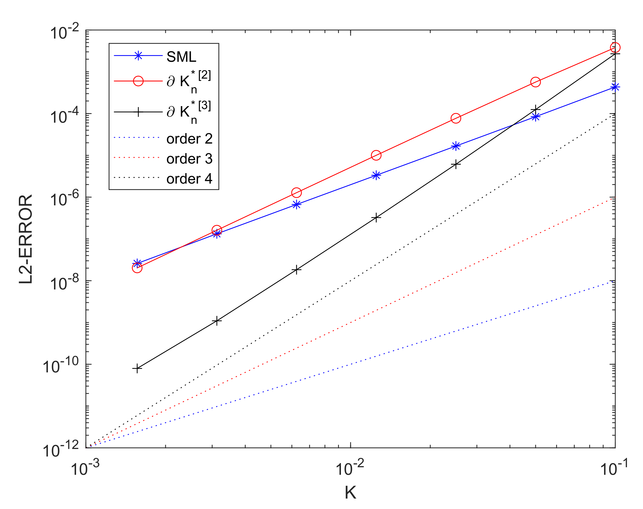
with h such that the exact solution of the above equation is $u(t,x)=e^{t+x^3}$. For the time integration, we have considered the Rosenbrock method GRK4T [22], which has four stages and does not satisfy condition (3.11) (or its equivalent (3.11)’) in [6]. Therefore, the standard method of lines leads to order 2 in time for this method [5]. For the space discretization, we have considered a Gauss-Lobatto collocation spectral method based on 41 nodes, which leads to negligible errors in space. We have implemented the method of lines, considering first the time discretization and then the space one. We have also considered the boundaries $\partial {K_n^{*}}^{\left[2\right]}$ and $\partial {K_n^{*}}^{\left[3\right]}$. We have measured the error committed when integrating until time $T=1$ in the discrete $L^2$-norm which is associated to the Gauss-Lobatto nodes. Figure 1 shows this error in terms of the chosen timestep. More precisely, asterisks (’*’) correspond to the standard method of lines, which makes first the space discretization and then the temporal one, circles (’o’) to the suggested method of lines with $G_n=\partial {K_n^{*}}^{\left[2\right]}$ and crosses (’+’) to $G_n=\partial {K_n^{*}}^{\left[3\right]}.$ As observed in the figure, the slope of the corresponding lines increases with the last two modifications, in such a way that the errors also become smaller, and the more the more the stepsize $k=1/n$ decreases. (Notice also that the cost of the last modifications is negligible compared with the total cost of the method because we are just acting on the boundary). In such a way, the classical order 4 of the method is recovered, as Table 1 shows more precisely.

Figure 1. Semilinear equation with $f(t,u)=u^2+h\left(t\right)$ and GRK4T integrator, with Dirichlet boundary conditions.

Table 1. Orders for global error, GRK4T and $f(t,u)=u^2+h\left(t\right)$ with Dirichlet boundary conditions. SML stands for ‘standard method of lines’ and $\partial {K_n^{*}}^{\left[2\right]}$, $\partial {K_n^{*}}^{\left[3\right]}$ for the different variations of the technique suggested in this paper.

n	5–10	10–20	20–40	40–80
SML	2.04	2.20	2.33	2.52
$\partial {K_n^{*}}^{\left[2\right]}$	2.81	2.91	2.96	2.99
$\partial {K_n^{*}}^{\left[3\right]}$	4.37	4.26	4.15	4.08

On the other hand, we have also considered a differential equation like that in (23), but with Dirichlet boundary condition just at $x=-1$, and at $x=1$, the Robin one

$$\begin{array}{c}\hfill u(t,1)+u_x(t,1)=4e^{t+1},\end{array}$$

(24)

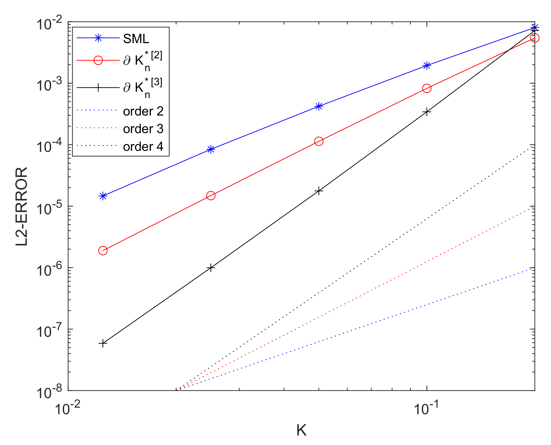
so that the exact solution of the problem continues to be $u(t,x)=e^{t+x^3}$. The implementation of the Robin boundary condition leads now to a Galerkin Gauss-Lobatto spectral discretization for the Lagrange polynomial associated to the last node ($x=1$), so that the numerical value at $x=1$ is now an additional unknown for the space discretization. In order to get now local order 4 with the suggested technique, we have had to resort to numerical differentiation in time to approximate the time derivative at that last node. We have done so through a Taylor method of order 2 for the first steps and through a 3-BDF formula for the consecutive ones. As Table 2 shows, the orders of the error with the different strategies considered in this paper are the same as those with Dirichlet boundary conditions although, as it can be observed in Figure 2, smaller stepsizes have to be considered so that the errors are smaller than those committed with the standard method of lines. This last remark is more obvious for $\partial {K_n^{*}}^{\left[2\right]}$. In any case, for stepsizes smaller than $5\times {10}^{-2}$, the suggested technique with $\partial {K_n^{*}}^{\left[3\right]}$ is clearly the one which leads to smaller errors.

Table 2. Orders for global error, GRK4T and $f(t,u)=u^2+h\left(t\right)$, with Robin boundary condition. SML stands for ‘standard method of lines’ and $\partial {K_n^{*}}^{\left[2\right]}$, $\partial {K_n^{*}}^{\left[3\right]}$ for the different variations of the technique suggested in this paper.

n	10–20	20–40	40–80	80–160	160–320	320–640
SML	2.36	2.33	2.33	2.32	2.33	2.36
$\partial {K_n^{*}}^{\left[2\right]}$	2.74	2.88	2.94	2.97	2.99	2.99
$\partial {K_n^{*}}^{\left[3\right]}$	4.43	4.35	4.24	4.15	4.06	3.78

Figure 2. Semilinear equation with $f(t,u)=u^2+h\left(t\right)$ and GRK4T integrator, with Robin boundary condition.

We have also considered a problem where the differential operator has variable coefficients, which is a case also included in the abstract formulation (1). More precisely, we have integrated

$$u_t(t,x)={\left(x^2{u}_x(t,x)\right)}_x+u^2+h(t,x),$$

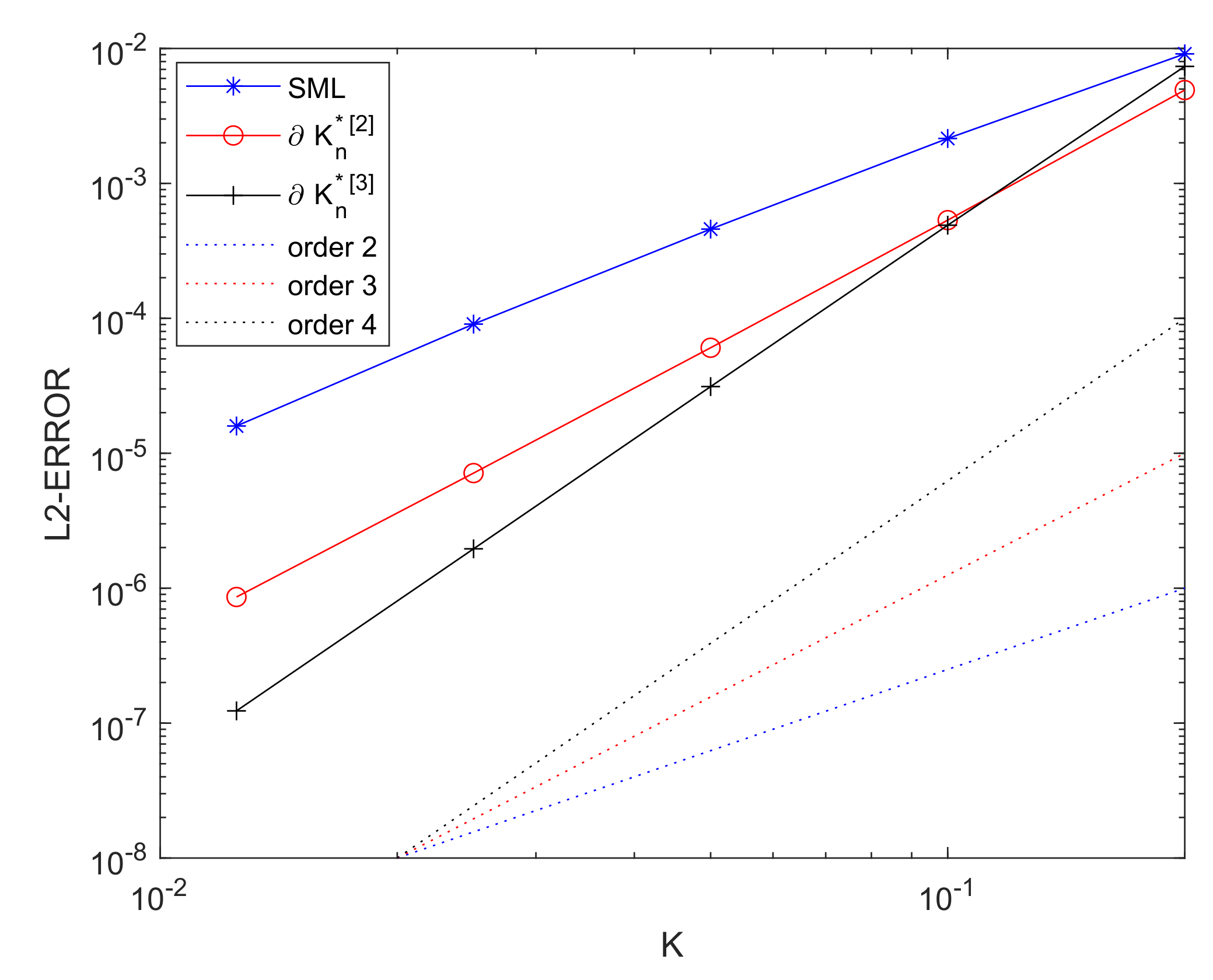
with Dirichlet boundary conditions so that again the exact solution is $u(x,t)=e^{t+x^3}$. The results are shown in Figure 3 and Table 3, where it is observed that the technique suggested with both $\partial {K_n^{*}}^{\left[2\right]}$ and $\partial {K_n^{*}}^{\left[3\right]}$ improves the order of the standard method of lines in the expected way.

Figure 3. Semilinear equation with $f(t,u)={\left(x^2{u}_x\right)}_x+h\left(t\right)$ and GRK4T integrator, with Dirichlet boundary conditions.

Table 3. Orders for global error, GRK4T and $f(t,u)={\left(x^2{u}_x\right)}_x+h\left(t\right)$ with Dirichlet boundary conditions. SML stands for ‘standard method of lines’ and $\partial {K_n^{*}}^{\left[2\right]}$, $\partial {K_n^{*}}^{\left[3\right]}$ for the different variations of the technique suggested in this paper.

n	5–10	10–20	20–40	40–80
SML	2.05	2.20	2.33	2.52
$\partial {K_n^{*}}^{\left[2\right]}$	2.73	2.86	2.93	2.97
$\partial {K_n^{*}}^{\left[3\right]}$	4.39	4.27	4.15	4.08

Let us now consider the equation,

$$\begin{array}{c}\hfill u_t(t,x)=u_{xx}(t,x)+u(t,x)u_x(t,x)+h(t,x),x\in [-1,1]\end{array}$$

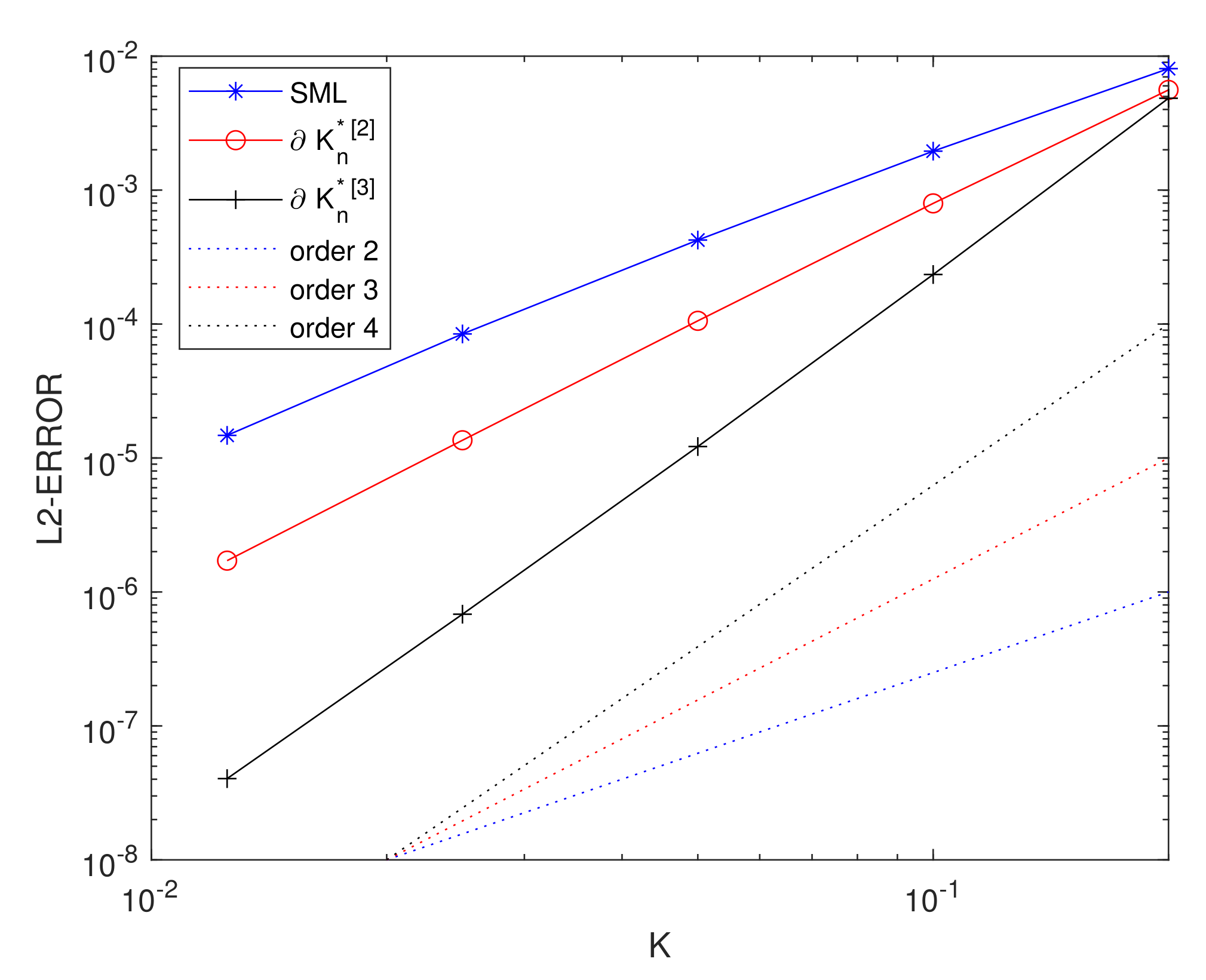
with h such that the exact solution of the above equation is again $u(t,x)=e^{t+x^3}$. We have integrated it with the same numerical methods than before and also considering Dirichlet boundary conditions. First, we have used the standard method of lines and then the suggested method of lines with $G_n=\partial {K_n^{*}}^{\left[2\right]}$. Finally, as $G_n=\partial {K_n^{*}}^{\left[3\right]}$ is not exactly calculable in terms of data as in problem (23) with Dirichlet boundary conditions, we have approximated those values through numerical differentiation following item 4 in Section 3.4. More explicitly, we have considered the 3-BDF formula to differentiate in time except for the first steps where Taylor series of order 2 is used taking Burger’s equation into account and the fact that the initial condition is known. Then, we have used differentiation in space of those values through Gauss-Lobatto collocation space discretization and its evaluation on the boundary. As expected, we have obtained order near 2 with the standard method of lines, order near 3 with $\partial {K_n^{*}}^{\left[2\right]}$ and order near 4 with $\partial {K_n^{*}}^{\left[3\right]}$. This can be observed in Figure 4 and Table 4.

Figure 4. Semilinear equation with $f(t,u)=u{u}_x+h\left(t\right)$ and GRK4T integrator, with Dirichlet boundary conditions.

Table 4. Orders for global error, GRK4T and $f(t,u)=u{u}_x+h\left(t\right)$. SML stands for ‘standard method of lines’ and $\partial {K_n^{*}}^{\left[2\right]}$, $\partial {K_n^{*}}^{\left[3\right]}$ for the different variations of the technique suggested in this paper.

n	5–10	10–20	20–40	40–80
SML	2.08	2.23	2.34	2.51
$\partial {K_n^{*}}^{\left[2\right]}$	3.20	3.14	3.09	3.05
$\partial {K_n^{*}}^{\left[3\right]}$	3.91	3.97	3.99	3.99

5. Conclusions

The paper thus provides a technique to avoid order reduction when integrating nonlinear problems with Rosenbrock methods, which is the kind of problems for which these methods were constructed. This technique is cheap when compared with the classic method of lines because additional terms must be added in the calculation of the stages, which imply the calculations of certain suitable boundary values for them. As the boundary grid values are negligible compared with those in the interior of the domain, the cost can also be considered negligible with respect to that of the whole method. We remark that numerical differentiation must be used to achieve a high enough order. That threshold order depends on the problem at hand and it happens that the higher the order to be pursued, the higher the order of the derivatives to approximate numerically, and therefore, the more probable that instability issues due to roundoff turn up. In any case, in the numerical experiments of the previous section, in which we managed to achieve order 4, we could not observe those instabilities. What’s more, to our knowledge, there is no other way to achieve that order for those type of problems when using Rosenbrock methods.

References

- Hairer, E.; Norsett, S.; Wanner, G. Solving Ordinary Differential Equations. I: Nonstiff Problems, 2nd ed.; Springer Series in Computational Mathematics, 8; Springer: Berlin, Germany, 1993. [Google Scholar]
- Hairer, E.; Wanner, G. Solving Ordinary Differential Equations. II: Stiff and Differential-Algebraic Problems, 2nd ed.; Springer Series in Computational Mathematics, 14; Springer: Berlin, Germany, 1996. [Google Scholar]
- Alonso–Mallo, I.; Cano, B. Spectral/Rosenbrock discretizations without order reduction for linear parabolic problems. Appl. Num. Math. 2002, 47, 247–268. [Google Scholar] [CrossRef]
- Lang, J.; Verwer, J.G. ROS3P—An accurate third-order Rosenbrock solver designed for parabolic problems. BIT 2001, 41, 731–738. [Google Scholar] [CrossRef]
- Lubich, C.; Ostermann, A. Linearly implicit time discretization of non-linear parabolic equations. IMA J. Numer. Anal. 1995, 15, 555–583. [Google Scholar] [CrossRef]
- Ostermann, A.; Roche, M. Rosenbrock methods for partial differential equations and fractional orders of convergence. SIAM J. Numer. Anal. 1993, 30, 1084–1098. [Google Scholar] [CrossRef]
- Ostermann, A.; Thalhammer, M. Non-smooth data error estimates for linearly implicit Runge-Kutta methods. IMA J. Numer. Anal. 2000, 20, 167–184. [Google Scholar] [CrossRef]
- Rang, J.; Angermann, L. New Rosenbrock W-methods of order 3 for partial differential algebraic equations of index 1. BIT 2005, 45, 761–787. [Google Scholar] [CrossRef]
- Schwitzer, F. W-methods for semilinear parabolic problems. Appl. Num. Math. 1995, 18, 351–366. [Google Scholar] [CrossRef]
- Calvo, M.P.; Frutos, J.; Novo, J. An efficient way to avoid the order reduction of linearly implicit Runge-Kutta methods for nonlinear IBVP’s. In Mathematical Modelling, Simulation and Optimization of Integrated Circuits; Antreich, K., Bulirsch, R., Gilg, A., Rentrop, P., Eds.; International Series of Numerical Mathematics Vol. 146; Birkhauser Verlag: Basel, Switzerland, 2003; pp. 321–332. [Google Scholar]
- Keeling, S.L. Galerkin/Runge-Kutta discretizations for semilinear parabolic equations. SIAM J. Numer. Anal. 1990, 27, 394–418. [Google Scholar] [CrossRef][Green Version]
- Calvo, M.P.; Palencia, C. Avoiding the order reduction of Runge–Kutta methods for linear initial boundary value problems. Math. Comput. 2002, 71, 1529–1543. [Google Scholar] [CrossRef][Green Version]
- Alonso–Mallo, I.; Palencia, C. On the convolutions operators arising in the study of abstract initial boundary value problems. Proc. R. Soc. Edinb. 1996, 126A, 515–539. [Google Scholar] [CrossRef]
- Palencia, C.; Alonso–Mallo, I. Abstract initial boundary values problems. Proc. R. Soc. Edinb. 1994, 124A, 879–908. [Google Scholar] [CrossRef]
- Colli Franzone, P.; Deuflhard, P.; Erdmann, B.; Lang, J.; Pavarino, L.F. Adaptivity in space and time for reaction-diffusion systems in electrocardiology. SIAM J. Sci. Comput. 2006, 28, 942–962. [Google Scholar] [CrossRef]
- Rang, J. Improved traditional Rosenbrock-Wanner methods for stiff ODEs and DAEs. J. Comp. Appl. Math. 2015, 286, 128–144. [Google Scholar] [CrossRef]
- Rang, J. The Prothero and Robinson example: Convergence studies for Runge-Kutta and Rosenbrock-Wanner methods. Appl. Num. Math. 2016, 108, 37–56. [Google Scholar] [CrossRef]
- Alonso–Mallo, I. Runge–Kutta methods without order reduction for initial boundary value problems. Numer. Math. 2002, 91, 577–603. [Google Scholar] [CrossRef]
- Cano, B.; Reguera, N. How to avoid order reduction when Lawson methods integrate reaction-diffusion initial boundary value problems. BIT Num. Math. 2021. [Google Scholar] [CrossRef]
- Cano, B.; Moreta, M.J. How to avoid order reduction when explicit Runge-Kutta exponential methods integrate reaction-diffusion initial boundary value problems. 2021; Submitted for Publication. [Google Scholar]
- Henry, D. Geometric Theory of Semilinear Parabolic Problems; Springer Lectures Notes in Mathematics, 840; Springer: Berlin, Germany, 1981. [Google Scholar]
- Kaps, P.; Rentrop, P. Generalized Runge-Kutta methods of order four with stepsize control for stiff ordinary differential equations. Numer. Math. 1979, 33, 55–68. [Google Scholar] [CrossRef]
Publisher’s Note: MDPI stays neutral with regard to jurisdictional claims in published maps and institutional affiliations. |
© 2021 by the authors. Licensee MDPI, Basel, Switzerland. This article is an open access article distributed under the terms and conditions of the Creative Commons Attribution (CC BY) license (https://creativecommons.org/licenses/by/4.0/).