Development of a Shipment Policy for Collection Centers

Abstract

Natural disasters represent a latent threat for every country in the world. Due to climate change and other factors, statistics show that they continue to be on the rise. This situation presents a challenge for the communities and the humanitarian organizations to be better prepared and react faster to natural disasters. In some countries, in-kind donations represent a high percentage of the supply for the operations, which presents additional challenges. This research proposes a Markov Decision Process (MDP) model to resemble operations in collection centers, where in-kind donations are received, sorted, packed, and sent to the affected areas. The decision addressed is when to send a shipment considering the uncertainty of the donations’ supply and the demand, as well as the logistics costs and the penalty of unsatisfied demand. As a result of the MDP a Monotone Optimal Non-Decreasing Policy (MONDP) is proposed, which provides valuable insights for decision-makers within this field. Moreover, the necessary conditions to prove the existence of such MONDP are presented.

1. Introduction

In a world where natural and man-made disasters are on the rise in both number and intensity, the efficiency of humanitarian operations gains importance in order to be prepared and respond efficiently to the communities’ needs. An estimated 80% of disaster relief operations involves making aid, food, and other resources available to the affected people in a timely and adequate manner [1], the very definition of logistics in the context of disaster relief supply chain.

An essential part of success in any supply chain is the policies and adequate management of the inventories at every echelon. In the case of disaster relief supply chains, proper inventory control ranges from the collecting centers to on-site distribution centers and the last mile distribution points and it can make a significant difference in attending to the affected communities in a timely and adequate fashion.

Classic inventory strategies and decision-making policies hardly adjust to the diverse conditions faced in a crisis such as properly responding to a natural disaster. This in turn challenges the researchers in the field of humanitarian logistics to develop customized policies, strategies, and models to efficiently manage the inventories of supplies in the specific case of emergency and disaster response [2,3].

In many countries, during the immediate aftermath of a disaster, some key inventory items are positioned at the origin of the relief supply chain through donations to the collection centers. For example, in Mexico, the percentage of in-kind donations received in the aftermath of a disaster can go up to 80% [4]. These donations range from human resources, housing, and medical supplies to food, clothing, and personal hygiene items, etc. They can also come through donations made by governments, the private sector or citizens.

Therefore, in-kind donations, can be the backbone of relief operations since they constitute a large percentage of the available resources to work with. However, they also create a high variable starting point for the disaster relief supply chain due to their arbitrary nature. Most of the research done in disaster relief operations assumes that the resources to be sent to the affected areas are in the quantity and nature required. Additionally, despite the importance of in-kind donations in some countries, little research has been conducted to address their efficient management and distribution. Donations that are addressed in the body of research on disaster relief operations are mostly financial.

Some researchers consider in-kind donations in disaster relief operations with an approach of material convergence problem [5,6], others research on the psychological drivers towards donating in cash or in-kind [7,8]. Only few authors such as Cook and Lodree [9] address this problem with the uncertainty of in-kind donations and the uncertainty in the demand. However, the research proposed by these authors, focuses solely on the minimization of the unsatisfied demand. For this research, we seek to integrate the goal of the minimization of the unsatisfied demand with the logistics costs that it entails.

Collection centers are usually installed by public organizations and private sectors to receive donations, and they can also function as a place of preparation, packaging, and transit of shipments. They may be located outside or within the affected region [10].

In this work, the operation of such collection centers was developed with the aim of developing efficient policies for their decision-making process. Depending on the strength and impact of the disaster, organizations may evaluate the suitability of opening and running collection centers for a certain period of time. In the case of this research, we attempt to address those events with a large enough impact to call for the necessity of nationwide aid collection. Hence, we assume that relief operations are being held at a national level and collection centers are positioned throughout the country.

Collection centers are confronted by the uncertainty in the quantity and nature of the in-kind donations that will be received daily and similarly, the quantity and nature of the aid that will be required in the affected areas. These two variables directly impact the operations conducted in the collection centers, and the decisions made regarding the size and frequency of the shipments, i.e., the dispatching policy of the donations to the affected areas. The research presented in this document addresses the creation of efficient decision-making policies to this end.

Making such a decision can become especially complicated when the costs of shipping and distribution are also added to the decision process. This decision is currently addressed by the stakeholders based mostly on their experience. They may send a shipment once the vehicle is full, which could take from one to several days to get to its destination, therefore, creating a lag in satisfying the demand. In other cases, the decision is made considering the demand alone, which can lead to making smaller shipments and ignoring the long-term cost implications.

The goal of this research was to develop a Markov Decision Process Model (MDP) to model the daily operations in collection centers. In addition, to make the decision of sending a shipment to the affected areas based on the available inventory and current accumulated demand, while considering the tradeoff between the implications of unsatisfied demand and the cost of frequent shipments. Such a model provides valuable insights to facilitate the analysis and, most importantly, decision-making among the key stakeholders involved in these operations.

The output of the MDP developed through this research is a policy or a sequence of decision rules where the decision, at any period of time, may depend on the available information on the system at the time [11]. This policy is derived for the developed MDP as a Monotone Optimal Non-Decreasing Policy (MONDP) after validating the necessary conditions for its existence. These conditions provide useful and valuable insights for decision makers in this field.

The remainder of this paper is organized as follows. Section 2 describes the details of the addressed problem. Section 3 presents the elements of the proposed Markov Decision Process Model. Section 4 states the conditions for the existence of a MONDP. In Section 5, these conditions are mathematically verified. Finally, Section 6 presents the conclusions as well as some future research.

2. Problem Description

This section presents the setting of the mathematical model including the problem statement, the notation used in the MDP model, and the sequence of events occurring in each period of time.

2.1. Problem Statement

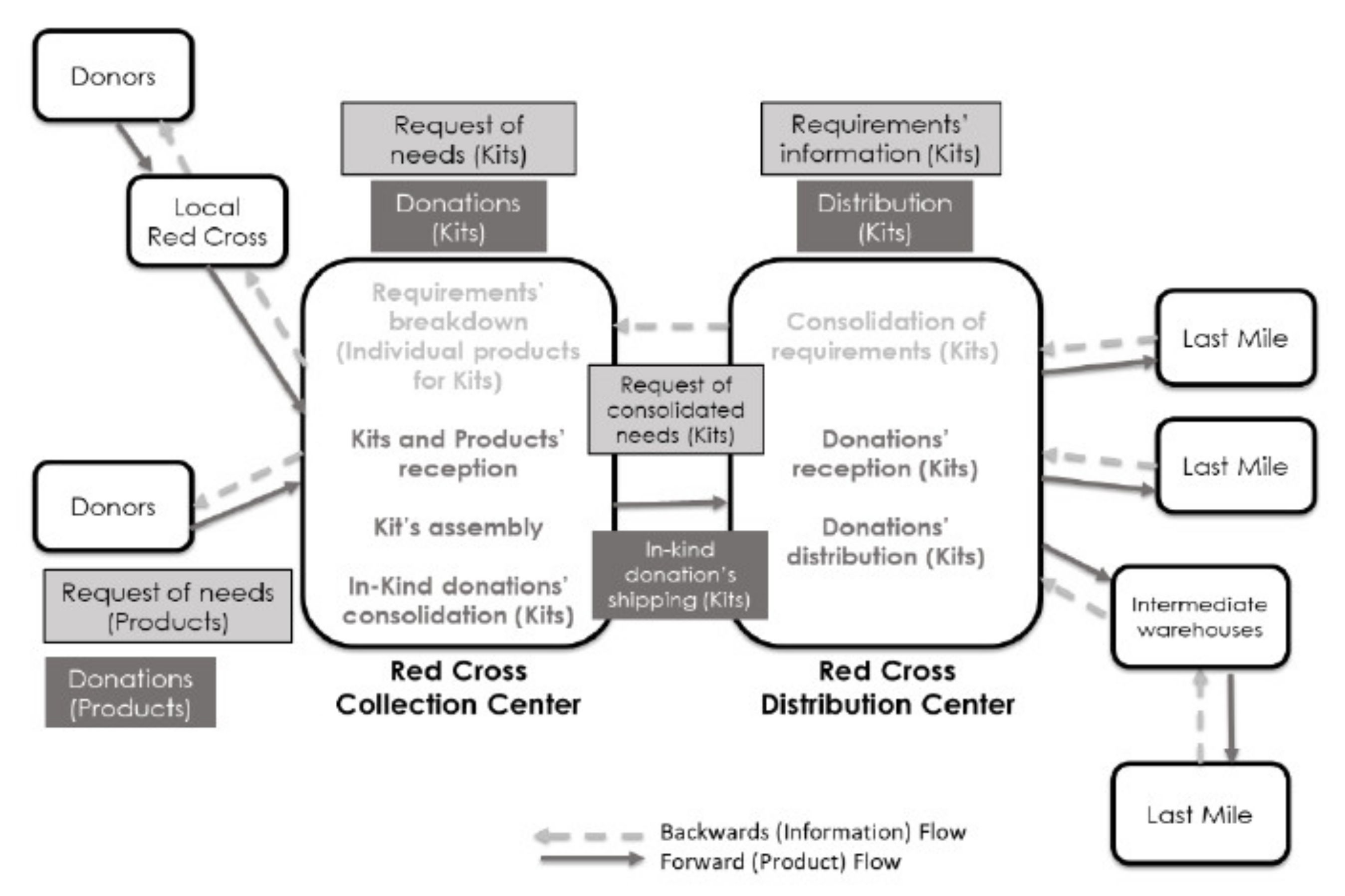
When a natural disaster strikes, and national assistance is required, different disaster relief protocols are put into place to respond to the emergency. One of them is to enable collection centers to receive in-kind donations. Figure 1 presents an example of a national disaster relief supply chain, based on our field observations working with the Mexican Red Cross operations.

The dotted lines going from right lo left represent the information flow along the supply chain from the affected areas to the donors. Information regarding the required good is initially assessed and constantly updated by the onsite team and travels up to potential donors. Donors (presented on the left of Figure 1) receive the requirements and seek to provide the different products to cover the assessed needs. The products are received through the collection centers, consolidated, sorted, and packed to be shipped to the onsite distribution center to eventually be distributed to smaller warehouses or directly to the points of distribution.

The Mexican Red Cross requires specific items to be packaged into predesigned aid kits such as food, hygiene, house cleaning or baby care kits. These aid kits have been predefined to work for one standard family and last for a specific period of time.

Therefore, in our model, we assume that in each decision epoch a random number of donations is received in the form of aid kits, increasing the available inventory, while the accumulated demand is updated when a request is received for a certain number of aid kits from the affected areas. The key decision is whether a shipment should be sent in the current period or not, while the size of the shipment is naturally defined based on the current available inventory and the accumulated demand.

2.2. Notation

This section presents the notation to be used in the formulation and validation of the MDP. Details of this notation are presented in

Table 1. Notation.

Notation	Definition	Type
$t$	Current decision epoch	Sub index
$d_t$	Number of kits demanded during period $t$	Random variable
$i_t$	Number of kits received during period $t$	Random variable
$a_t$	Action chosen at the beginning of decision epoch $t$	Actions
$Q_t$	Size of a shipment sent to the affected area at the beginning of decision epoch $t$. It is defined by the available inventory and the accumulated demand.	Variable
$D_t$	Cumulative unsatisfied demand (in number of kits) in the affected area at the beginning of decision epoch $t$	State Variable
$I_t$	Inventory on hand at the beginning of decision epoch $t$	State Variable
$I_t^f$	Inventory on hand at the beginning period $t$ is at level f
$T$	Length of the decision-making time horizon	Parameter
$N$	Total number of families located in the affected area	Parameter
$W$	Maximum number of kits that can be managed at the collection center at any given period	Parameter
$s_t$	Proportion of the families that will demand a kit at the beginning of period $t$	Parameter
$\mu$	Average number of donors that donate each period	Parameter
$\lambda$	Average amount of kits donated per donor	Parameter
$c_1$	Penalty cost for each unit (kit) of unmet demand per period.	Parameter
$c_2$	Fixed shipping cost that will be paid independently of the size of the shipment	Parameter
$c_3$	Variable shipping cost that depends on the number of kits sent.	Parameter
$c_4$	Cost for holding inventory at the collection center for one stage.	Parameter
$c_5$	Salvage value of the kits left in the collection center on the last period.	Parameter
$D_t^{*}$	Optimal level of demand to send a shipment at the beginning of period $t$	Variable
$p_t\left(I_{t+1}|\left(I_t,D_t\right),a_t\right)$	Probability of arriving to state $I_{t+1}$ given that there is currently $\left(I_t,D_t\right)$. and action $a_t$ was chosen	Transition Probability Function
$q_t\left(D_{t+1}|\left(I_t,D_t\right),a_t\right)$	Probability of arriving to state $D_{t+1}$ given that there is currently $\left(I_t,D_t\right)$ and action $a_t$ was chosen	Transition Probability Function
$P_t\left(\left(I_{t+1},D_{t+1})|(I_t,D_t\right),a_t\right)$	The joint probability of arriving to state $\left(I_{t+1},D_{t+1}\right)$ given the current state $\left(I_t,D_t\right)$ and action $a_t$ was chosen	Joint transition probability
$r_t\left(\left(I_t,D_t\right),a_t\right)$	Total cost incurred in period t when inventory and demand are $\left(I_t,D_t\right)$ respectively and action $a_t$ chosen	Cost Function
$r_T\left(I_T,D_T\right)$	Cost incurred in final period when no decision is made	Cost Function for final period
$u_t\left(I_t,D_t\right)$	Accumulated Value of having certain inventory and demand up to time $t$	Value Function

.

2.3. Sequence of Events

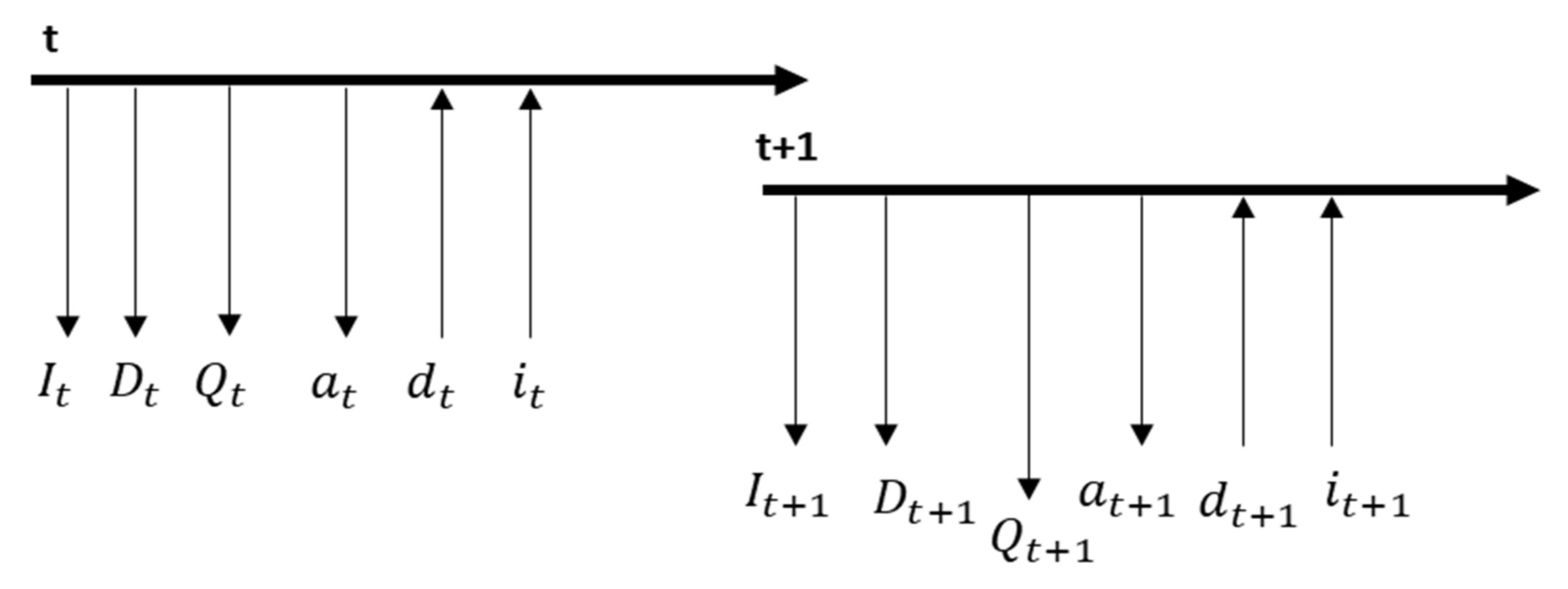
Figure 2 presents the graphical description in each discrete period of time, with a number of the sequence of events occurring throughout the decision process, and the description of each event follows.

• The $t^{th}$ period starts with the information of the inventory on hand and the accumulated demand $\left(I_t,D_t\right)$.
• The size of the possible shipment is calculated by the available inventory and the accumulated demand up to period t. The shipment size is computed as follows:

  $$Q_t=\min \left\{I_t,D_t+E\left[d_t\right]\right\}$$

  (1)
• Once the size of the shipment is determined, the decision maker can choose an action ($a_t)$, which consists of whether to send a shipment of size $Q_t$ or not to send a shipment at that period.
• After making the decision, up to the end of the current period new donations ($i_t$) are received and the demand of that period ($d_t$) also arrives.
• By the end of the day, the collection center closes and opens the next day, starting a new period t+1.
• Starting a new period t+1 the available inventory ($I_{t+1}$) and accumulated demand ($D_{t+1}$) are updated with the information of the previous period, adding the new donations and demand and subtracting the sent donations. In the case that the action taken was not to send, $Q_t$ will be zero. This update is computed as follows:

  $$I_{t+1}=I_t+i_t-Q_t$$

  (2)

  $$D_{t+1}=D_t+d_t-Q_t$$

  (3)
• With this updated information, as in period t, the shipment decision is made for any $t$.

3. Markov Decision Process Model

This section presents the Markov Decision Process Model proposed for the collection center operations. It starts with the assumptions under which the model was developed and continues with the five elements of the MDP model, as well as the value function to be minimized.

3.1. Assumptions

• In the addressed problem, we are looking at a finite horizon, discrete time setting with length T. The value of T is determined by the decision-maker based on several factors such as the type of disaster, the scope of the impact on the affected population, etc.
• Time is discrete and each of the time epochs or stages (t) can represent one working day or any period that fits the scenario.
• It is assumed that the random variable of the available inventory ($I_t)$ and accumulated demand $(D_t)$ are Markovian and their values only depend on the previous inventory, previous demand, and the action ($a_t)$ taken in the previous period. This is a reasonable assumption, given the nature and dynamics of inventory management and shipments made under these kinds of events. New inventory levels will depend on random donations and shipments that took place in the previous period.
• The total number of families in the affected area (N) is known at the beginning of the emergency, although not all of them are necessarily in need of rescue or response. This can be known by the population census owned by the government and is a free access for organizations.
• The affected population that generates the demand of the collection center can be modelled as a binomial random variable ($q_t)$, since each family demands a kit, independently of the situation faced by the other affected families [12,13]. This implies having a certain probability of families out of N that will demand a kit in period $t$ ($s_t$).

  $$d_t~Bin\left(N,s_t\right)$$
• The average number of donors ($\mu$) and the average amount of donations per donor ($\lambda$) are defined based on the type of disaster that took place and the specific characteristics of the affected population.
• The approximate proportion of the families that will demand a kit in period t ($s_t$) and the behavior of this proportion throughout the time horizon can be estimated by the organization. This value depends mostly on two factors: The socioeconomic status of the affected region (i.e., if the socioeconomic level is low the demand will be higher) and the second factor is the impact of the disaster, according to the Florida Post-Disaster Redevelopment Planning Guidebook (2010).
• The number of kits received during a period t ($i_t$) is modeled as a Compound Poisson Process, since the number of donors arriving in each period is random, as well as the amount of donations they will provide.

  $$i_t~DCP\left(\mu \lambda \right)$$
• The initial inventory is zero since all the prepositioned products are assumed to be sent in the initial response phase.
• The shipments are made for national disasters, therefore, the shipping time is considered to be one day, and it is assumed that the shipment arrives complete.
• The transition probability function for demand $q_t\left(d_t|\left(I_t,D_t\right),a_t\right)$ is the increasing failure rate (IFR). In the context of our problem, this means that the higher the demand, the more probable that the demand will keep increasing.
• For this model, it is considered that the shipment cannot be much larger than the current demand. This is due to the fact that having a surplus of supplies can compromise their integrity since they are exposed to theft and damage.

Limitations in transport capacity are not considered in this MDP. This is due to the fact that during the interviews carried out with the leader of the Mexican Red Cross, it has not been a core boundary since they not only have their own truck fleet, but they have an agreement with the government and some multinationals such as Walmart to assist with their infrastructure, if necessary.

It is also worth mentioning that, considering the operations of the Mexican Red Cross, standard kits are designed according to the population’s basic needs, considering the average family size and eating habits of the country. The design and use of kits happens also at an international level with the International Federation of the Red Cross. There may be other items demanded beyond these kits, in which supply, including donations, and demand may be handled by other organizations supporting the affected population.

3.2. Decision Epochs

Our decision epochs are assumed to be discrete stages where the decision is made at the beginning of each epoch t and T − 1 is the last epoch when a decision is made. Therefore, the last shipment would be sent in T − 1 if the decision for that last epoch dictates so.

$$t\in \left\{0,1,2,\dots ,T-1\right\}$$

3.3. State Variables

The state of the system in each period t is defined by the tuple $(I_t,D_t)$. $I_t$ describes the inventory on hand at stage t which is suitable to be sent to the affected area.

$$I_t\in \left\{0,1,\dots ,W\right\}$$

This variable carries the accumulated donations from period 1 minus the quantity of kits sent in the previous periods and is computed as presented in Equation (4). This equation is equivalent to the Equation (2) previously introduced.

$$I_t={{\displaystyle \sum }}_{j=1}^{t-1}\left(i_j-Q_j\right)$$

(4)

The second variable $D_t$, describes the cumulative unsatisfied demand (in number of kits) in the affected area at stage t. The ordered elements of $D_t$ are represented as:

$$D_t\in \left\{0,1,\dots ,N\right\}$$

This variable carries the cumulative demand from the beginning minus the number of kits that have already been shipped in the previous periods and is computed as follows:

$$D_t={{\displaystyle \sum }}_{j=1}^{t-1}(d_j-Q_j)$$

(5)

The states of the system are grouped by the level of inventory and are partially ordered according to the accumulated demand.

3.4. Actions

The goal of the MDP is to decide whether to send a shipment in period t. This decision is made at the beginning of the period and has the following two possible alternatives.

The action $a_t=\left\{0\right\}$ represents the decision of not sending a shipment in the current period. This implies that the available inventory will continue to be stocked in the collection center for one more period and the demand will be accumulated for one more period, as well.

The action $a_t=\left\{1\right\}$ represents sending a shipment of size $Q_t$ in the current period. The size of the shipment depends on the current available inventory and the current demand. If the available inventory is less than the accumulated demand, the shipment will be the size of the inventory trying to satisfy as much demand with what is available. On the other hand, if the inventory is greater than the demand, the shipment will be the size of the accumulated demand plus the expected demand of the next period. The size of the shipment is previously presented in Equation (1).

3.5. Transition Probabilities

The transition probabilities for this model are composed of two independent probabilities since the model includes two state variables: The available inventory $\left(I_t\right)$ and the accumulated demand $\left(D_t\right)$. These two variables have different and independent behaviors, therefore are modelled separately and then a joint probability function is presented.

3.5.1. Donations Probability Function

$p_t\left(I_{t+1}|\left(I_t,D_t\right),a_t\right)$ is the probability of reaching to the state of $I_{t+1}$ donations, given that the current state is $\left(I_t,D_t\right)$ and action $a_t$ is taken.

As presented in assumption 8, the value of the received donations in period t ($i_t$) is modeled as a Compound Poisson Process. The value of $i_t$ directly impacts the state variable of the available inventory for the next period $\left(I_{t+1}\right)$. Therefore, the state space for the next period depends on the current state, the action taken, and the donations received.

In the case of choosing action 0, not sending a shipment in that period, the possible future states depend exclusively on the number of donations received ($i_t$). Hence, the future states will have the current amount plus the received donations $\left(I_t+i_t\right)$. The possible states can go from having no donations whatsoever and the inventory level stays in $\left(I_t\right)$ to receiving the necessary amount of donations to filling the collection’s center capacity ($W$).

For the case of choosing action 1, sending a shipment of size $Q_t$, the possible future states will depend on the size of the shipment made ($Q_t$) and the quantity of donations received ($i_t$). The future states could range from the remaining inventory after the shipment $\left(I_t-Q_t\right)$, assuming there are no additional donations, to the full capacity of the collection center, considering that they received $W-\left(I_t-Q_t\right)$.

Since in both cases there is a limited number of feasible states in the state space, the traditional Compound Poisson Distribution is adjusted to its conditional probability by dividing it by the probabilities of the feasible states.

The probability function is computed as follows:

For $a_t=\left\{0\right\}$:

$$p_t\left(I_t+i_t|\left(I_t,D_t\right),0\right)=\left\{\begin{array}{cc}\raisebox{1ex}{${\left(\mu *\lambda \right)}^{i_t}\times \frac{e^{-\mu *\lambda }}{i_t!}$}\!\left/ \!\raisebox{-1ex}{${{\displaystyle \sum }}_{i_t=0}^{W-I_t}\mu \times {\lambda }^{i_t}\times \frac{e^{-\mu \times \lambda }}{i_t!}$}\right.& ifW-I_t\ge i_t\ge 0\\ 0& otherwise\end{array}\right.$$

(6)

For $a_t=\left\{1\right\}$:

$$p_t\left(I_t+i_t-Q_t|\left(I_t,D_t\right),1\right)=\left\{\begin{array}{cc}\raisebox{1ex}{${\left(\mu *\lambda \right)}^{i_t}\times \frac{e^{-\mu *\lambda }}{i_t!}$}\!\left/ \!\raisebox{-1ex}{${{\displaystyle \sum }}_{i_t=0}^{W-\left(I_t-Q_t\right)}\mu \times \lambda {)}^{i_t}\times \frac{e^{-\mu \times \lambda }}{i_t!}$}\right.& ifW-\left(I_t-Q_t\right)\ge i_t\ge 0\\ 0& otherwise\end{array}\right.$$

(7)

3.5.2. Demand Probability Function

$q_t\left({\mathrm{D}}_{\mathrm{t}}|\left(I_t,D_t\right),{\mathrm{a}}_t\right)$ is the probability of arriving at state $D_{t+1}$ kits demanded, given that the current state is $\left(I_t,D_t\right)$ and action $a_t$ was chosen.

As presented in assumption 6, the value of the demanded kits in period t ($d_t$) is modeled as a binomial random variable, where $s_t$ represents the probability of a family requesting a kit at time t. The value of $d_t$ directly impacts the state variable of the available inventory to be sent for the next period $\left(I_{t+1}\right)$. Therefore, the state space for the next period depends on the current state, the action taken, and the donations received.

Similar to the case of available inventory, the feasible future states are determined by the current state, the action taken, and the demand in period t. For the case of choosing action 0, the demand will continue increasing and the possible states will range from the current demand (considering that no more kits were demanded during that period) to the total number of families in the affected area ($N$), assuming each would need a kit.

In the case of action 1 (i.e., sending a shipment of size $Q_t$), the possible future states are divided in two categories that depend directly on the size of the shipment: (a) If the shipment sent is greater than the accumulated demand in period t or (b) if the shipment is less than or equal to the accumulated demand in period t.

In case (a), all the demand will be satisfied completely and there will be extra inventory after satisfying the demand. Therefore, the possible future state can go from having zero accumulated demand, considering that the demand in the next period is less than or equal to the remaining shipment, to having the maximum demand possible. The maximum demand possible is the total number of families N minus the number of families that have been served with the shipment.

In case (b), the demand was not completely satisfied. Therefore, the future states will be staying in the same level of demand, i.e., $d_t$ is equal to zero, to having all the families that were not served with $Q_t$ demanding kits.

The probability distribution function is computed as:

For $a_t=\left\{0\right\}$:

$$q_t\left(D_t+{\mathrm{d}}_t|\left(I_t,D_t\right),0\right)=\left\{\begin{array}{cc}\left(\begin{array}{c}N-D_t\\ d_t\end{array}\right)s_t{}^{d_t}{\left(1-s_t\right)}^{N-D_t-d_t}& \mathrm{if}N-D_t\ge d_t\ge 0\\ 0& otherwise\end{array}\right.$$

(8)

For $a_t=\left\{1\right\}$:

$$q_t\left(D_t+d_t-Q_t|\left(I_t,D_t\right),1\right)=\left\{\begin{array}{c}a)if{Q}_t>D_t\\ b)if{Q}_t\le D_t\end{array}\right.$$

For case a:

$$q_t\left(D_t+d_t-Q_t|\left(I_t,D_t\right),1\right)=\left\{\begin{array}{cc}{{\displaystyle \sum }}_{d_t=0}^{Q_t-D_t}\left(\begin{array}{c}N-D_t\\ d_t\end{array}\right)s_t^{d_t}{\left(1-s_t\right)}^{N-D_t-d_t}& if0\le d_t<Q_t-D_t\\ \left(\begin{array}{c}N-D_t\\ d_t-\left(Q_t-D_t\right)\end{array}\right)s_t^{d_t-\left(Q_t-D_t\right)}{\left(1-s_t\right)}^{N-D_t-d_t-\left(Q_t-D_t\right)}& if{Q}_t-D_t\le d_t\le N-Q_t\end{array}\right.$$

(9)

For case b:

$$q_t\left(D_t+d_t-Q_t|\left(I_t,D_t\right),1\right)=\left\{\begin{array}{cc}\left(\begin{array}{c}N-D_t\\ d_t\end{array}\right)s_t^{d_t}{\left(1-s_t\right)}^{N-D_t-d_t}& if0\le d_t\le N-D_t\\ 0& otherwise\end{array}\right.$$

(10)

3.5.3. Joint Transition Probability Function

$P_t\left(\left(I_{t+1},D_{t+1})|(I_t,D_t\right),a_t\right)$ represents the joint probability of having a certain amount of demand and donations given the current state and the action taken. This is the product of the independent probabilities $p_t\left(i_t|\left(I_t,D_t\right),a_t\right)$ and $q_t\left({\mathrm{d}}_{\mathrm{t}}|\left(I_t,D_t\right),{\mathrm{a}}_t\right)$, as follows:

$$P_t\left(\left(I_{t+1},D_{t+1})|(I_t,D_t\right),a_t\right)=p_t\left(I_t|\left(I_t,D_t\right),a_t\right)\times q_t\left(D_t|\left(I_t,D_t\right),a_t\right)$$

(11)

3.6. Cost Function

$r_t\left(\left(I_t,D_t\right),a_t\right)$ is the total immediate cost incurred in period t when action $a_t$ is taken.

The cost function for action 1 is formed by: The cost of the unsatisfied demand, in case there is any, after the shipment is delivered in the first term, the fixed and variable costs of sending a shipment in the second and third terms, finally the cost of holding the rest of the inventory, if any, in the last term.

On the other hand, the cost function for action 0 is formed by the cost of unsatisfied accumulated demand in the first term and the holding cost of the available inventory at the collection center.

$$r_t\left(\left(I_t,D_t\right),a_t\right)=\left\{\begin{array}{cc}{c}_1{\left(D_t-Q_t\right)}^{+}+c_2+c_3\left(Q_t\right)+c_4\left(I_t-Q_t\right)& fora=1\\ c_1(D_t)+c_4\left(I_t\right)& fora=0\end{array}\right.$$

(12)

$r_T\left(I_T,D_T\right)$ is the immediate cost incurred in the final period, when no decision is made.

$$r_T\left(I_T,D_T\right)=c_1(D_T)-c_5(I_T)$$

(13)

3.7. Value Function

This problem can be formulated as the following optimality equations:

$$u_t\left(I_t,D_t\right)=mi{n}_{a\in A}\left\{r_t\left(\left(I_t,D_t\right),a_t\right)+{\displaystyle \sum }_{j=0}^N{P}_t\left(\left(I_{t+1},D_{t+1})|(I_t,D_t\right),a_t\right)\times u_{t+1}^{*}\left(I_{t+1},D_{t+1}\right)\right\}\hspace{1em}\forall I_t$$

(14)

$$\begin{gathered} u_t\left(I_t,D_t\right)=mi{n}_{a\in A}\left\{c_1(D_t)+c_4\left(I_t\right)+{\displaystyle \sum }_{j=D_{t-1}}^N{p}_t\left(I_{t+1}|\left(I_t,D_t\right),0\right)\times q_t\left(D_j^{t+1}|\left(I_t,D_t\right),0\right)\times u_{t+1}\left(I_{t+1},D_{t+1}\right)c_1{\left(D_t-Q_t\right)}^{+}+c_2+c_3\left(Q_t\right)+c_4\left(I_t-Q_t\right)+{\displaystyle \sum }_{j=0}^N{p}_t\left(I_{t+1},|\left(I_t,D_t\right),1\right)*q_t\left(\left(D_j^{t+1}\right)|\left(I_t,D_t\right),1\right),\times u_{t+1}\left(I_{t+1},D_{t+1}\right)\right\} \\ \mathrm{For}\mathrm{t}=1,2,\dots \mathrm{T}-1\mathrm{and}\forall I_t \end{gathered}$$

(15)

$$u_T\left(I_T,D_T\right)=\begin{array}{cc}{r}_T\left(I_T,D_T\right)& \forall I_t\end{array}$$

(16)

4. Monotone Optimal Non-Decreasing Policy

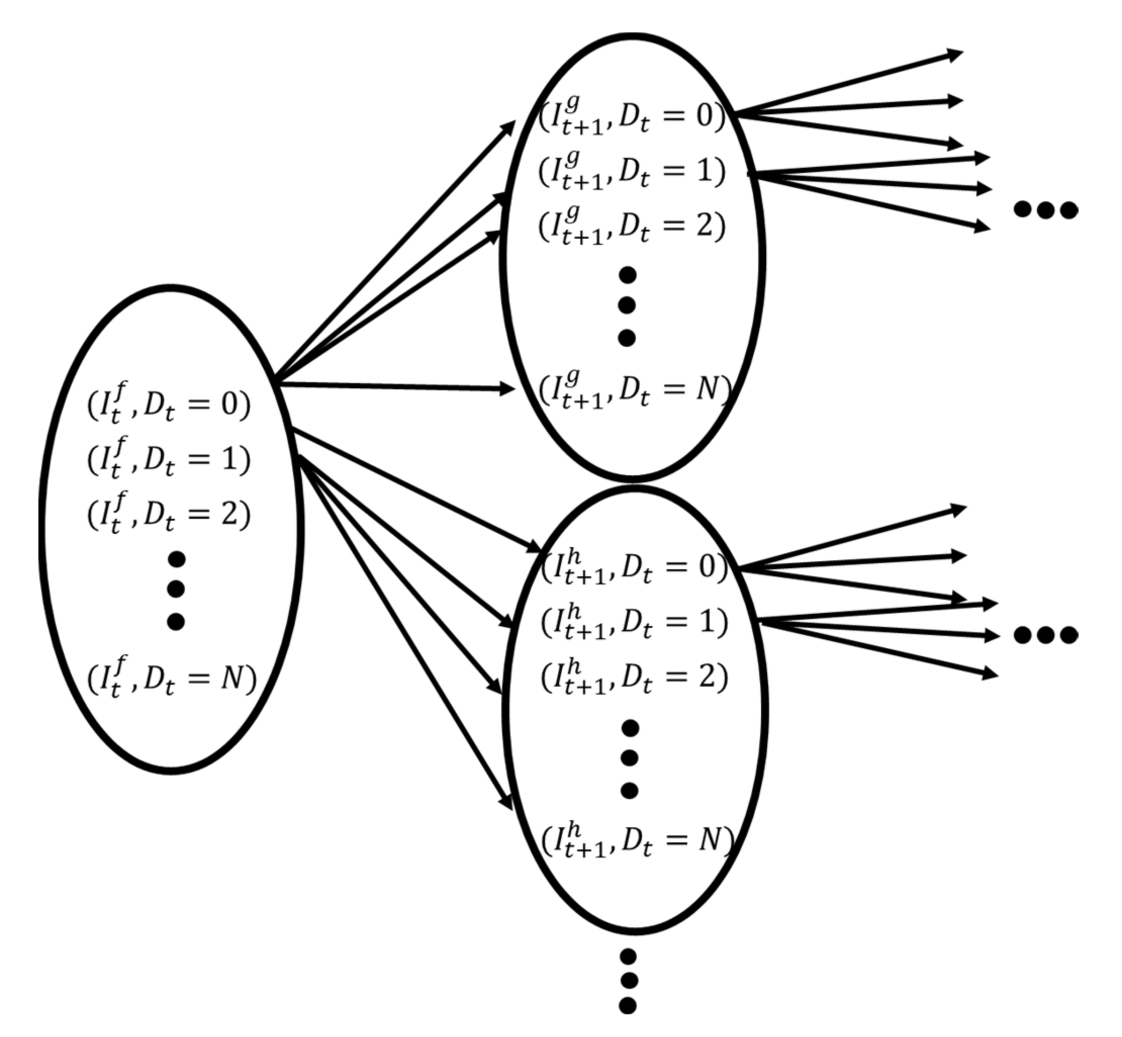
To establish the set of conditions to assure that a Monotone Optimal Nondecreasing Policy (MONDP) exists, a physical interpretation and a natural ordering of the states is necessary. In this case, the states are ordered by the accumulated unsatisfied demand ($D_t$), i.e., a larger size of unsatisfied demand represents a higher level in the states of the system. Figure 3 visually represents the behavior of the partially ordered groups.

The groups are formed according to the current level of inventory, since the availability of inventory determines the maximum shipment size to cover the demand. Therefore, it depends on the level of the demand if the shipment is sent in that period.

Each group of states ($I_t,D_t$) is partially ordered according to the following criteria:

• At each period of time t, a group of states with different values of $I_t$ is generated. They are defined as $I_t^f,I_t^g,\dots$ according to the number of kits currently available in the collection center at time t.
• Each group of states generated at time t, has a logical order according to the levels of the accumulated non-satisfied demand $D_t$.

In the MONDP, the threshold where the action of “not sending” changes to “send” is represented by a control limit with the following structure, where $D_t^{*}$ represents the demand level from where it is optimal to start sending:

$$a_t=\left\{\begin{array}{c}0\left(I_t,D_t\right)<\left(I_t,D_t^{*}\right)\\ 1\left(I_t,D_t\right)\ge \left(I_t,D_t^{*}\right)\end{array}\right.$$

(17)

Theorem 4.7.4 of Puterman [14] provides conditions under which there exist monotone nondecreasing optimal policies in all the states for t = 1,…,T−1. These conditions presented in the context of our problem are:

• $u_t\left(\left(I_t,D_t\right),a_t\right)$ is non-decreasing in $\left(D_t\right)$ for $a_t=\left\{0,1\right\}$.
• $q_t\left({\mathrm{D}}_{\mathrm{t}}|\left(I_t,D_t\right),{\mathrm{a}}_t\right)$ is non-decreasing in $\left(D_t\right)\forall I_t$ and $a_t=\left\{0,1\right\}$.
• $u_t\left(\left(I_t,D_t\right),a_t\right)$ is a superadditive function in $\left(I_t,D_t\right)\times a_t$.
• $q_t\left({\mathrm{D}}_{\mathrm{t}}|\left(I_t,D_t\right),{\mathrm{a}}_t\right)$ is a superadditive function in $\left(D_t\right)\times a_t$.
• $u_T\left(I_T,D_T\right)$ is non decreasing in $\left(I_T,D_T\right)$.

5. Mathematical Verification for the MOND Policy

For a setting to present this monotone behavior, it is necessary but not sufficient to meet the conditions mentioned in the previous section. The setting of the problem must meet the model parameters that fit the policy, as well.

The mathematical proof of the five conditions and the lemmas that sustain them are presented in this section.

5.1. Condition 1

Equation (8) a is non-decreasing in ($D_t$) for each level of inventory $I_t$ and action a = 0. This implies that the cost incurred in the collection center will increase with the increase of the accumulated unsatisfied demand for any fixed level of inventory.

For a = 0 and for all $I_t$

$$u_t\left[\left(I_t,D_t\right),0\right]\le u_t\left[\left(I_t,D_t+1\right),0\right]$$

(18)

$$c_1\left(D_t\right)+c_4\left(I_t\right)+{{\displaystyle \sum }}_{j=D_t}^N{P}_{t+1}\left(\left(I_{t+1},D_j^{t+1}\right)|\left(I_t,D_t\right),0\right)\times r_{t+1}\left(\left(I_{t+1},D_j^{t+1}\right),0\right)\le c_1\left(D_t+1\right)+c_4\left(I_t\right)+{{\displaystyle \sum }}_{j=D_t+1}^N{P}_{t+1}\left(\left(I_{t+1},D_j^{t+1}\right)|\left(I_t,D_t+1\right),0\right)\times r_{t+1}\left(\left(I_{t+1},D_j^{t+1}\right),0\right)$$

This condition implies that the larger the accumulated demand $D_t$ (in number of kits), under the decision of not sending, the higher the costs will be.

$$c_1\left(\left(D_t+1\right)-D_t\right)+{\displaystyle \sum }_{j=D_t+1}^N{P}_{t+1}\left(\left(I_{t+1},D_j^{t+1}\right)|\left(I_t,D_t+1\right),0\right)\times r_{t+1}\left(\left(I_{t+1},D_j^{t+1}\right),0\right)-{{\displaystyle \sum }}_{j=D_t}^N{P}_{t+1}\left(\left(I_{t+1},D_j^{t+1}\right)|\left(I_t,D_t\right),0\right)\times r_{t+1}\left(\left(I_{t+1},D_j^{t+1}\right),0\right)]\ge 0$$

This reduces to:

$$c_1\left(1\right)+{\displaystyle \sum }_{j=D_t+1}^N{P}_{t+1}\left(\left(I_{t+1},D_j^{t+1}\right)|\left(I_t,D_t+1\right),0\right)\times r_{t+1}\left(\left(I_{t+1},D_j^{t+1}\right),0\right)-{{\displaystyle \sum }}_{j=D_t}^N{P}_{t+1}\left(\left(I_{t+1},D_j^{t+1}\right)|\left(I_t,D_t\right),0\right)\times r_{t+1}\left(\left(I_{t+1},D_j^{t+1}\right),0\right)]\ge 0$$

This inequality stands since $r_t\left(I_t,D_t\right)<r_t\left(I_t,D_t+1\right)$.

5.2. Condition 2

Condition 2 states that $q_t[\left(D_{t+1}=D_l\right)|\left[\left(I_t,D_t\right),a_t\right]$ is a non-decreasing function in $\left(D_t\right)$ $\forall D_l$ and $a_t=\left\{0,1\right\}$. In the context of the problem, this implies that the probability of having a higher accumulated demand in the next period is more when the current accumulated demand is high.

This condition is stated as follows:

$$\begin{gathered} q_t[\left(I_t,D_{t+1}=D_l\right)|\left[\left(I_t,D_t\right),a_t\right]\le q_t[\left(I_t,D_{t+1}=D_l\right)|\left[\left(I_t,D_t+i\right),a_t\right] \\ where1\le i\le N-D_t \end{gathered}$$

(19)

In this instance, there are three possible cases:

Case 1: $D_l<D_t$ for $a_t$ = 0.

Case 2: $D_t\le D_l\le D_t+i$ for $a_t$ = 0.

Case 3: $D_t+i<D_l$ for $a_t$ = 0.

Case 1

In the first case, the accumulated unsatisfied demand in t−1 is greater than $D_l$ for both sides of the inequality. The probability of the accumulated unsatisfied demand being higher than or equal to $D_t$ is 1. Therefore, the inequality is satisfied as an equality.

Case 2

In the second case, the accumulated unsatisfied demand is higher than $D_l$ in the right-hand side of the inequality so, the probability of having at least $D_l$ in the next period is 1. Therefore, the inequality corresponding to case 2 is satisfied independently of the value of the probability term on the left-hand side since the maximum value is 1.

Case 3

The condition can be stated as:

$${\displaystyle \sum }_{d_t=D_l-D_t}^{N-D_t}\left(\begin{array}{c}N-D_t\\ d_t\end{array}\right)s_t^{d_t}{\left(1-s_t\right)}^{N-D_t-d_t}\le {\displaystyle \sum }_{d_t=D_l-\left(D_t+i\right)}^{N-\left(D_t+i\right)}\left(\begin{array}{c}N-\left(D_t+i\right)\\ d_t\end{array}\right)s_t^{d_t}{\left(1-s_t\right)}^{N-(D_t+i)-d_t}$$

(20)

It can be rewritten as:

$$1-{\displaystyle \sum }_{d_t=0}^{D_l-D_t-1}\left(\begin{array}{c}N-D_t\\ d_t\end{array}\right)s_t^{d_t}{\left(1-s_t\right)}^{N-D_t-d_t}\le 1-{\displaystyle \sum }_{d_t=0}^{D_l-\left(D_t+i\right)-1}\left(\begin{array}{c}N-\left(D_t+i\right)\\ d_t\end{array}\right)s_t^{d_t}{\left(1-s_t\right)}^{N-(D_t+i)-d_t}$$

$${\displaystyle \sum }_{d_t=0}^{D_l-D_t-1}\left(\begin{array}{c}N-D_t\\ d_t\end{array}\right)s_t^{d_t}{\left(1-s_t\right)}^{N-D_t-d_t}\ge {\displaystyle \sum }_{d_t=0}^{D_l-\left(D_t+i\right)-1}\left(\begin{array}{c}N-\left(D_t+i\right)\\ d_t\end{array}\right)s_t^{d_t}{\left(1-s_t\right)}^{N-(D_t+i)-d_t}$$

Equation (11) represents the comparison between two random variables X and Y as defined in Lemma 1 as:

$$P\left(X\le D_l-D_t-1\right)\ge P\left(Y\le D_l-D_t-1-i\right)$$

(21)

This inequality is proved through Lemma 1. With this, Condition 2 is verified as one of the conditions of the existence of a Monotone Optimal Nondecreasing Policy.

5.3. Proof of Lemma 1

Recall that $X_n$ is a binomial random variable with parameters n and p, where n = 1,2, … and 0 < p < 1. Its expected value is ${\mu }_n=E\left[X_n\right]=np$. Therefore, for any n, m = 1,2, …, n−1 and for any integer there is:

$$\begin{gathered} P\left(X_n>l\right)\ge P\left(X_m>l\right) \\ for0\le l\le m \end{gathered}$$

(22)

Proof:

Consider $P\left(X_n>l\right)-P(X_{n-1}>l)$ where l is an integer. Therefore:

$$P\left(X_n>l\right)-P\left(X_{n-1}>l\right)=\left[P\left(X_{n-1}>l\right)+P\left(X_{n-1}=l\right)\times P\left(U=1\right)\right]-P(X_{n-1}>l)$$

$$\begin{gathered} \left(\begin{array}{c}n-1\\ l\end{array}\right)p^{l+1}{\left(1-p\right)}^{n-1-l}>0 \\ where{X}_n=X_{n-1}+U \end{gathered}$$

This implies that the probability to experience more than l successes is greater when an additional experiment is added to the sequence of Bernoulli trials.

$$P\left(X_n>l\right)-P\left(X_{n-1}>l\right)>0$$

This relation can be scaled with a random value of n as:

$$\begin{gathered} P\left(X_{n-1}>k\right)-P\left(X_{n-2}>k\right)>0 \\ P\left(X_{n-2}>k\right)-P\left(X_{n-3}>k\right)>0 \\ \dots \end{gathered}$$

By transitivity we have:

$$P\left(X_n>k\right)-P\left(X_m>k\right)>0forl=1,2,\dots ,n-1\hspace{1em}■$$

5.4. Condition 3

Condition 3 requires $Equation8.a$ to be a superadditive function. Puterman states that this happens when we have partially ordered sets X and Y and $g\left(x,y\right)$ is a real valued function on $X\times Y$. A superadditive function then holds the following inequality:

$$g\left(x^{+},y^{+}\right)+g\left(x^{-},y^{-}\right)\ge g\left(x^{+},y^{-}\right)+g\left(x^{-},y^{+}\right)$$

(23)

Condition 3, following Puterman’s definition, for $Equation8.a$ can be expressed as follows:

$$u_t\left[\left(I_t,D_t\right),1\right]+u_t\left[\left(I_t,D_t+1\right),0\right]\le u_t\left[\left(I_t,D_t\right),0\right]+u_t\left[\left(I_t,D_t+1\right),1\right]$$

(24)

To demonstrate that Equation (8) a is superadditive it is be shown that both Equation (7) a and ${\sum }_{j=0}^N{P}_{t+1}\left(\left(I_{t+1},D_j^{t+1})|(I_t,D_t\right),a_t\right)\times u_{t+1}^{*}\left(I_{t+1},D_{t+1}\right)$ are superadditive. Proposition 1 demonstrates that it is superadditive.

Proposition 1

The function $r_t\left(\left(I_t,D_t\right),a_t\right)$ is superadditive. This is represented as:

$$r_t\left(\left(I_t,D_t\right),1\right)+r_t\left(\left(I_t,D_t+1\right),0\right)\ge r_t\left(\left(I_t,D_t\right),0\right)+r_t\left(\left(I_t,D_t+1\right),1\right)$$

(25)

Proof:

$$c_1{\left(D_t-Q_t\right)}^{+}+c_2+c_3\left(Q_t\right)+c_4\left(I_t-Q_t\right)+c_1(D_t+1)+c_4\left(I_t\right)\ge c_1(D_t)+c_4\left(I_t\right)+c_1{\left(D_t+1-Q_t\right)}^{+}+c_2+c_3\left(Q_t\right)+c_4\left(I_t-Q_t\right)$$

$$c_1{\left(D_t-Q_t\right)}^{+}+c_1(D_t+1)\ge c_1(D_t)+c_1{\left(D_t+1-Q_t\right)}^{+}$$

This instance presents two possible cases:

• Case 1:

  $$\begin{gathered} {\left(D_t-Q_t\right)}^{+}\le 0 \\ {c}_1\left(0\right)+c_1(D_t+1)\ge c_1(D_t)+c_1\left(0\right) \\ {c}_1(D_t+1)\ge c_1(D_t) \end{gathered}$$

  This statement is true, therefore, the condition is met.
• Case 2:

  $$\begin{gathered} {\left(D_t-Q_t\right)}^{+}>0 \\ {c}_1\left(D_t-Q_t\right)+c_1(D_t+1)\ge c_1(D_t)+c_1\left(D_t+1-Q_t\right) \\ {c}_1{D}_t-c_1{Q}_t+c_1{D}_t+c_1\ge c_1{D}_t+c_1{D}_t+c_1-c_1{Q}_t \\ 0=0 \end{gathered}$$

Proposition 2

Function $\sum _{j=0}^N{P}_{t+1}\left(\left(I_{t+1},D_j^{t+1})|(I_t,D_t\right),a_t\right)\times u_{t+1}^{*}\left(I_{t+1},D_{t+1}\right)$ is superadditive.

$${\displaystyle \sum }_{j=0}^N{P}_{t+1}\left(\left(I_{t+1},D_j^{t+1})|(I_t,D_t+1\right),0\right)\times u_{t+1}^{*}\left(I_{t+1},D_j^{t+1}\right)\ge {\displaystyle \sum }_{j=0}^N{P}_{t+1}\left(\left(I_{t+1},D_j^{t+1})|(I_t,D_t\right),0\right)\times u_{t+1}^{*}\left(I_{t+1},D_j^{t+1}\right)$$

(26)

$${\displaystyle \sum }_{j=0}^N{P}_{t+1}\left(\left(I_{t+1},D_j^{t+1})|(I_t,D_t\right),1\right)\times u_{t+1}^{*}\left(I_{t+1},D_j^{t+1}\right)\ge {\displaystyle \sum }_{j=0}^N{P}_{t+1}\left(\left(I_{t+1},D_j^{t+1})|(I_t,D_t+1\right),1\right)$$

For A and B.

Proof by Lemma 2

$${\displaystyle \sum }_{j=0}^N{P}_{t+1}\left(\left(I_{t+1},D_j^{t+1})|(I_t,D_t+1\right),0\right)\times u_{t+1}^{*}\left(I_{t+1},D_j^{t+1}\right)+{\displaystyle \sum }_{j=0}^N{P}_{t+1}\left(\left(I_{t+1},D_j^{t+1})|(I_t,D_t\right),1\right)\times u_{t+1}^{*}\left(I_{t+1},D_j^{t+1}\right)\ge {\displaystyle \sum }_{j=0}^N{P}_{t+1}\left(\left(I_{t+1},D_j^{t+1})|(I_t,D_t\right),0\right)*u_{t+1}^{*}\left(I_{t+1},D_j^{t+1}\right)+{\displaystyle \sum }_{j=0}^N{P}_{t+1}\left(\left(I_{t+1},D_j^{t+1})|(I_t,D_t+1\right),1\right)\times u_{t+1}^{*}\left(I_{t+1},D_j^{t+1}\right)$$

which is superadditive by the previously stated definition and the assumed grouping and ordering of states and actions, thus completing the proof.

Proof of Lemma 2 (Adopted from [15]):

Let $\mathcal{H}$ be an IFR transition probability matrix and V(h) be a nondecreasing function. Then, the following holds:

$$a){\displaystyle \sum }_{h^{\prime }\le h}\left[\mathcal{H}\left(h^{\prime }|h\right)-\mathcal{H}\left(h^{\prime }|h+1\right)\right]V\left(h^{\prime }\right)\le {\displaystyle \sum }_{h^{\prime }\le h}\left[\mathcal{H}\left(h^{\prime }|h\right)-\mathcal{H}\left(h^{\prime }|h+1\right)\right]V\left(h\right)$$

(27)

$$b){\displaystyle \sum }_{h^{″}>h}\left[\mathcal{H}\left(h^{″}|h\right)-\mathcal{H}\left(h^{″}|h+1\right)\right]V\left(h^{″}\right)\le {\displaystyle \sum }_{h^{\prime }\le h}\left[\mathcal{H}\left(h^{″}|h\right)-\mathcal{H}\left(h^{″}|h+1\right)\right]V\left(h+1\right)$$

(28)

Proof for (a). The IFR assumption implies that ${{\displaystyle \sum }}_{i=1}^{h^{\prime }}\mathcal{H}\left(i|h\right)\ge {{\displaystyle \sum }}_{i=1}^{h^{\prime }}\mathcal{H}\left(i|h+1\right)$ for any $h^{\prime }\in S_H$. Now,

$${{\displaystyle \sum }}_{h^{\prime }\le h}\left[\mathcal{H}\left(h^{\prime }|h\right)-\mathcal{H}\left(h^{\prime }|h+1\right)\right]V\left(h^{\prime }\right)\ge 0$$

$$\left[\mathcal{H}\left(1|h\right)-\mathcal{H}\left(1|h+1\right)\right]V\left(1\right)+{\displaystyle \sum }_{h^{\prime }=2}^h\left[\mathcal{H}\left(h^{\prime }|h\right)-\mathcal{H}\left(h^{\prime }|h+1\right)\right]V\left(h^{\prime }\right)\le \left[\mathcal{H}\left(1|h\right)-\mathcal{H}\left(1|h+1\right)\right]V\left(2\right)+{\displaystyle \sum }_{h^{\prime }=2}^h\left[\mathcal{H}\left(h^{\prime }|h\right)-\mathcal{H}\left(h^{\prime }|h+1\right)\right]V\left(h^{\prime }\right)$$

(29)

$$\left[\mathcal{H}\left(1|h\right)+\mathcal{H}\left(2|h\right)-\mathcal{H}\left(1|h+1\right)-\mathcal{H}\left(2|h+1\right)\right]V\left(2\right)+{\displaystyle \sum }_{h^{\prime }=3}^h\left[\mathcal{H}\left(h^{\prime }|h\right)-\mathcal{H}\left(h^{\prime }|h+1\right)\right]V\left(h^{\prime }\right)\le \left[\mathcal{H}\left(1|h\right)+\mathcal{H}\left(2|h\right)-\mathcal{H}\left(1|h+1\right)-\mathcal{H}\left(2|h+1\right)\right]V\left(3\right)+{\displaystyle \sum }_{h^{\prime }=2}^h\left[\mathcal{H}\left(h^{\prime }|h\right)-\mathcal{H}\left(h^{\prime }|h+1\right)\right]V\left(h^{\prime }\right)$$

where this equation follows due to $\mathcal{H}\left(1|h\right)\ge \mathcal{H}\left(1|h+1\right)$ and $V\left(1\right)\le V\left(2\right)$. We obtain the second inequality by restating the first, and the last inequality holds due to $\mathcal{H}\left(1|h\right)+\mathcal{H}\left(2|h\right)\ge \mathcal{H}\left(1|h+1\right)+\mathcal{H}\left(2|h+1\right)$ and $V\left(2\right)\le V\left(3\right)$. The result follows if we apply the same procedure to states 3 through h.

Proof for (b). The proof is similar to the proof of Part (a) and is omitted.

5.5. Condition 4

This condition states that Equation (5) a is a superadditive function in $\left(I_t,D_t\right)\forall D_l\times a_t$, which implies that the difference between the probability of having a given number of demand when not sending and sending a certain shipment, does not decrease when the cumulative demand increases.

This can be written as:

$$q_{t+1}[\left(D_l\right)|\left(I_t,D_t^{+}\right),1)\left]-q_{t+1}\right[\left(D_l\right)|\left(I_t,D_t^{+}\right),0)\left]\le q_{t+1}\right[\left(D_l\right)|\left(I_t,D_t^{-}\right),1)\left]-q_{t+1}\right[\left(D_l\right)|\left(I_t,D_t^{-}\right),0)]$$

(30)

where $D_t^{+}>D_t^{-}$.

Since the value of the demand does not depend on the on-hand inventory and it does not change for each inventory group, this condition is satisfied as an equality.

5.6. Condition 5

Equation (7) c is non-decreasing in $\left(I_T,D_T\right)$. This implies that the final cost is greater when the accumulated demand in T is greater.

$$u_T\left(I_T,D_T\right)=r_T\left(I_T,D_T\right)$$

(31)

$$\begin{gathered} r_T\left(I_T,D_T\right)\le r_T\left(I_T,D_T+i\right) \\ \mathrm{Where}1\le i\le n \end{gathered}$$

$$\begin{gathered} c_1(D_T)-c_5(I_T)\le c_1(D_T+i)-c_5(I_T) \\ 0\le i \end{gathered}$$

As presented in this section, the five conditions Puterman states for the existence of a Monotone Optimal Non-Decreasing Policy are mathematically validated, proving the existence of such policy for the shipment decision in collection centers.

6. Conclusions

Natural disasters present a latent threat for every country in the world, challenging the communities and the humanitarian organizations to be better prepared and react faster to the situation. Along with the government and the humanitarian organizations, citizens also either volunteer or are asked to help with their donations.

In many countries, including emerging economies such as Mexico, around 80% are in-kind. Therefore, the efficient management of in-kind donations has become a key element of disaster relief operations in such countries. Other countries, especially in developing economies, present a similar donations behavior and, in consequence, suitability for implementation of the insights and recommendations presented through this research.

With the importance of in-kind donations, comes the importance of collection centers, where these donations are received, sorted, packed, and shipped to the affected areas. An important decision made is when to make the shipment, considering the tradeoff between resources limitations and the urgency of aids. This tradeoff is addressed by developing a decision process model.

Within their operations, collection centers face a high level of demand uncertainty, as well as the supply side since it mainly depends on the donations of companies or the community. This complex problem was modeled with a Markov Decision Process to address the uncertainty and complexity of the decision-making process. A Monotone Optimal Non-Decreasing Policy is developed for the use of decision makers.

The existence of such a policy is mathematically proved by five conditions and the verification of such conditions is presented throughout this paper. The proof of these conditions and the MONDP represents a valuable insight for decision makers in humanitarian operations since it helps in making better decisions in times of crisis.

Among the limitations of this work, which present useful avenues for future research, are the parameters and assumptions considered to estimate the number of donors and the average amount of donations per donor. Moreover, the proportion of families that may demand a kit at a particular point in time can be further improved by considering other factors beyond the socioeconomic status of the impacted region. In a similar manner, the number of kits received during a particular period can be modeled beyond a Compound Poisson Process to explore the system dynamics under such conditions.

This research can motivate further research in inventory management for disaster relief situations, especially considering the particularities and considerations that need to be taken for in-kind donations, such as variability and variety. Moreover, the link with humanitarian organizations and using real-time data, presents an important line of research for future applications of this model.