A Methodology for Redesigning Networks by Using Markov Random Fields

Abstract

Standard methodologies for redesigning physical networks rely on Geographic Information Systems (GIS), which strongly depend on local demographic specifications. The absence of a universal definition of demography makes its use for cross-border purposes much more difficult. This paper presents a Decision Making Model (DMM) for redesigning networks that works without geographical constraints. There are multiple advantages of this approach: on one hand, it can be used in any country of the world; on the other hand, the absence of geographical constraints widens the application scope of our approach, meaning that it can be successfully implemented either in physical (ATM networks) or non-physical networks such as in group decision making, social networks, e-commerce, e-governance and all fields in which user groups make decisions collectively. Case studies involving both types of situations are conducted in order to illustrate the methodology. The model has been designed under a data reduction strategy in order to improve application performance.

1. Introduction

Network redesigning is a dynamic problem that arises in several fields. The wide range of reasons for redesigning includes the need to adapt to changing requirements (new regulatory scenarios, for instance) or to enhance the sector’s capacities [1,2,3]. Not only is the further expansion of the network considered, but also reductions may be provided. Likewise, redesigning affects a large number of sectors in which networks play a role: apart from areas with standard branch networks (banking institutions, supermarkets and petrol or gas stations), it concerns the telecommunications and electricity sectors, transport industries by land, sea and air and many others in which the consideration of physical networks is required [4].

Redesigning processes go much further than adapting to changes as they involve several factors. However, at their core, all these variables may be considered to be within two main groups: (i) identifying operational shortfalls and (ii) projecting future performance in order to anticipate future needs. The latter concern could be interpreted as re-distributing nodes in the network (adding, removing and merging nodes) and assessing the results for each possibility. This paper is related to the latter concept: an approach is developed to model the evaluation of the future performance of a network in different scenarios in order to design the future network structure.

Standard methodologies for redesigning physical networks rely on Geographic Information Systems [5,6], which strongly depend on local specifications. However, the absence of a universal definition of demography makes the joint use of such technologies in domestic and international scenarios more difficult, especially for cross-border enterprises. Our contribution is to present a Decision Making Model to restructure networks that works without geographical constraints. More specifically, the novelty of our model is that local geographical specifications are optional (they could be included if required by the specific context) instead of compulsory. There are multiple advantages of our approach: on one hand, it may be used in any country of the world; on the other hand, there is a broad application scope, as our approach could successfully be implemented either in physical (ATM networks [7]) or in non-physical networks such as e-commerce, e-governance and all fields in which user groups make decisions collectively [8,9,10].

An additional contribution is that the model has been designed under a data reduction strategy (i.e., only significant information is required) in order to improve application performance. The advantages of this vary from reducing the storage space to increasing the speed of the decision-making model. Specifically, our approach is based on a joint probability distribution, which can be expressed as function of a few significant nodes of the network, called the cliques. While the employment of probability functions in decision-making models is not new (they have been widely used by Bayesian-based techniques), the novelty of our approach relies on the choice of Markov random fields instead of Bayesian networks as a supporting structure [11].

As a previous stage to the decision model itself, a universal (geographical constraint-free) network is overlapped with the given network. Such a universal network is constructed from the selected criteria for redesigning in such a way that if multiple criteria were needed, the methodology may be executed in parallel for all the considered criteria, thereby enhancing the decision capabilities of the model. Besides, the independence of the processes guarantees that the model may monitor the application performance automatically, without the figure of a driver (a moderator in GDM contexts, for instance; see [12,13]. As a result, different levels of precision can be simultaneously considered.

Related works on Markov fields include [14,15], where Markov Decision Processes are the tools used to analyze the given information in order to make decisions. In [16], Markov networks are the framework used to develop a scoring function (called BJP) that computes the joint posterior distribution of the collection of Markov blankets.

Network redesigning may be addressed from several standpoints and is usually related to a given criteria and performed by means of many techniques. In [17], the authors presented a branch redesigning framework by means of integer 0–1 programming, the objective of which is to restructure the network after mergers and takeovers. Other approaches rely on Fuzzy Cognitive Maps (FCMs) [18], in which a dynamic network of interconnected knowledge nodes is designed through the use of FCMs. The authors could not find any previous works which jointly addressed the restructuring of both physical and non-physical networks.

The organization of the paper is as follows. Section 2 provides an overview of Markov random fields. Section 3 and Section 4 are devoted to the decision-making model. Specifically, in Section 3, the pre-processing steps are established (Section 3.1 shows the construction of the universal network and Section 3.2 shows its resulting properties), while in Section 4, the decision-making model itself is developed. In Section 5 and Section 6, some applications are presented (Section 5: the banking context, Section 6: group decision making problems). Finally, Section 7 concludes the paper.

2. Preliminaries on Markov Random Fields

In the beginning, Graph Theory was devoted to finding walks and paths (Euler, Hamilton), but it is now used to find substructures (communities) in networks. As this is also the philosophy that underlies this paper, let us briefly review Markov random fields by starting with Graph Theory.

In a graph $G=(V,E)$ (V represents the set of vertices (nodes or sites) and E represents the set of edges), two vertices $u,v$ are said to be adjacent, $u\sim v$, if $(u,v)\in E$. Thus, the collection of adjacent vertices to a given vertex u is called the neighborhood of u, $N\left(u\right)=\{v\in V|u\sim v\}$. In this regard, it is well-known that defining a neighborhood is equivalent to defining the set E. Cliques in a graph are communities (subgraphs) of fully connected nodes: $C\subseteq V$ is a clique if $C\subseteq \{u,N(u\left)\right\},\forall u\in C$.

Depending on whether the edges are bidirectional or not, graphs are called undirected or directed. Those graphs whose nodes are random variables $X_v,v\in V$ and whose edges show statistical relationships with nodes are called graphical models. Graphical models over an undirected graph are called Markov random fields (MRFs), while Bayesian networks are graphical models whose underlying graph is a directed one.

MRFs may be also viewed as spatial networks that fulfill an extension of the Markov chains’ memory-less property. More specifically, Markov chains are linear random processes $\left\{X_n\right|n\in \mathbb{N}\}$ in which the probability of occurrence of each state $X_n$ depends solely on the immediately previous state $X_{n-1}$:

$$P[X_n=x_n|X_k=x_k,\forall k\ne n]=P[X_n=x_n|X_{n-1}=x_{n-1}].$$

Now, let us consider a spatial random process $X=\left\{X_v\right|v\in V\},V=\{1,2,\dots ,n\}\times \{1,2,\dots ,n\}$, and let $P\left[X\right]$ denote the joint distribution of X in the following sense: $P\left[X\right]=P\left[\{X_v=x_v|v\in V\}\right]=\left\{P[X_v=x_v]\right|v\in V\}.$, $X=\left\{X_v\right|v\in V\}$ is an MRF if the probability of a state depends solely on the nearest states, on the understanding that the nearest nodes are those that are in the neighborhood N:

$$P[X_v=x_v|X_{V-\left\{v\right\}}=x_{V-\left\{v\right\}}]=P[X_v=x_v|X_{N\left(v\right)}=x_{N\left(v\right)}].$$

For our purposes, it is important to highlight that the joint probability distribution of an MRF X takes a specific form provided that $P\left[X\right]\ge 0$. Particularly, it may be written in terms of functions that only take values on cliques of the network (called clique potentials), as follows:

$$P\left[X\right]=\frac{1}{Z}\prod _{C\in \mathcal{C}}{\varphi }_C\left(X_C\right),Z=\sum \prod _{C\in \mathcal{C}}{\varphi }_C\left(X_C\right),$$

where functions ${\varphi }_C\left(X_C\right)$ over the cliques $C\in \mathcal{C}$ are the clique potentials and Z is a normalization constant. In Gibbs distribution contexts, the normalizing constant Z is also known as the partition function. Its primary role is to ensure that the joint distribution sums to 1. While such a function ${\varphi }_C$ may take several forms, these are usually ${\varphi }_C\left(X_C\right)=exp(-f\left(C\right))$, with $f\left(C\right)$ being a function known as an energy function on C. Thus, the joint distribution of an MRF X may be expressed as

$$P\left[X\right]=\frac{1}{Z}exp\left[-\sum _{C\in \mathcal{C}}f\left(C\right)\right].$$

In Image modeling and processing, such a joint probability distribution is called a Gibbs distribution, and it gives its name to those spatial random processes whose full distribution is similar to the one above. These are known as Gibbs random fields and, following the Hammersley–Clifford theorem, they are essentially the same as MRFs.

3. The Redesigning Process: Pre-Processing Steps

The required steps in the redesigning process may be mainly divided into pre-processing steps and the decision-making model itself, according to Section 3.1 and Section 3.2.

3.1. Creation of a Universal Support Network ${(X_v,N_v)}_{v\in V}$

This section presents the design of a support network that is overlapped with the original one in order to granulate the original set of nodes depending on the selected criteria for redesigning. This support network is called universal in the sense that it works without local constraints. Let $(V,E)$ be the network that we aim to restructure according to a selected criterium. $(V,E)$ could be either physical or non-physical: in physical networks, nodes are physically connected, while in the non-physical contexts, edges are abstract links (for instance, friendships in social networks or business relationships in market scenarios). Thus, the steps to follow are as follows:

(i) A random variable X related to the criterion for redesigning should be selected. For example, in the case of restructuring a bank branch network under the criterion of branch size (as shown in Section 5), we have to select the random variable which best gathers the main features of the branch size.

(ii) Construct a support network ${(X_v,N_v)}_{v\in V}$. To achieve our goal, each node in the original network $v\in V$ produces a node in the support network $X_v$ when v is identified with the random variable $X_v$ tailored to v and extensively detailed by a collection of features $x_v^k,k=1,\dots ,n$; i.e., $v\sim X_v\simeq {(x_v^1,x_v^2,\dots ,x_v^n)}^t.$

From now on, both terms $v\sim X_v$ shall be used indistinctly. Note that in $X_v$, the vector coordinates (which represent the features $x_v^k,k=1,\dots ,n$) and their number can be chosen as needed. As mentioned in the Introduction, in the universal support network ${(X_v,N_v)}_{v\in V}$, local geographical specifications are optional if required by the specific context. Actually, they may be included as part of the features of the random variable X. We refer to $X_v$ as a variable-in-a-site, thereby providing a set of random variables $X=\{X_v\mid v\in V\}$.

Definition 1.

Consider nodes $X_{v_i}={(x_{v_i}^1,\dots ,x_{v_i}^n)}^t$, $X_{v_j}={(x_{v_j}^1,\dots ,x_{v_j}^n)}^t$ $i\ne j$ in the support network, and let $\overline{X_{v_i}}$ be the mean value in a given interval of time. The distance between $X_{v_i},X_{v_j},$ $i\ne j$, written as $d_{ij}$, is

$$\begin{array}{ccc}{d}_{ij}=d(v_i,v_j)(=d(X_{v_i},X_{v_j}))\hfill & =& +\sqrt{{\sum }_{k=1}^n{({\overline{x^k}}_{v_i}-{\overline{x^k}}_{v_j})}^2}.\hfill \end{array}$$

(1)

Remark 1.

Recall that the realization of a random variable X is the process of taking a concrete value $x_v$ over the full range of values that may be considered: $X_v=x_v$. In this regard, the mean value is a choice of realization of the random variable, but many other choices may be considered instead depending on what best suits each particular context. The definition of distance may be freely selected as well.

Definition 2.

The neighborhood of a node $v_i\in V$, $N_{v_i}$, is defined as

$$N_{v_i}=\{v_j\in V|d(v_i,v_j)\le k,k\in \mathbb{R},k\ne 0\},$$

where the benchmark k (which states the degree of similarity) must be specifically defined.

Note that, due to the equivalence between defining edges in a graph and a topology through a system of neighborhoods, edges in the support network ${(X_v,N_v)}_{v\in V}$ are now defined: for $v_j\in N\left(v_i\right)$, an edge ($v_i,v_j$) will be joined if $d(v_i,v_j)\le k\ne 0$. It should be noticed that Definition 2 could be seen as a more general definition of a neighborhood (a multi-hop neighborhood; see [19]).

3.2. Properties

In this section, some of the properties of the universal support network are described. Firstly, let us describe the nature of the neighborhood of a random variable:

Proposition 1

(Neighborhoods). The neighborhood of a random variable-in-a-site is formed by random variables that are very similar with regard to the selected criterion for redesigning the network.

Proof. 

Having identified every node with its set of features (according to the selected criterion) and considering that the benchmark k may be as small as desired, the former definition of a neighborhood implies that all random variables in a neighborhood are similar to the selected features. □

Proposition 2

(Cliques). A clique C in the universal network ${(X_v,N_v)}_{v\in V}$ (and in the original network $(V,E)$ as well) is a community which consists of those nodes $c_1^i,c_2^i$ that are highly similar with respect to the features of the random variable $X_v$; i.e., $d(c_1^i,c_2^i)\le k_i,i=1,2.$

Proof. 

The result follows from the fact that the nodes in a clique are also in the corresponding neighborhoods. Then, $d(c_1^i,c_2^i)\le min\{k_1,k_2\}\le k_1,k_2$. □

Remark 2.

Note that the selection of X directly affects the type of network categorization in the sense that for each choice of the random variable X, there is an associated network re-configuration. It is also important to note that the level of similarity for nodes in each $C_i$ is variable; i.e., nodes $c_1^i,c_2^i\in C_i$ are similar with degree $k_i$ while $c_1^j,c_2^j\in C_j$ may be similar with different degrees of similarity $k_i\ne k_j$ if $i\ne j$ (an instance of this is the Internet (the universal network), in which a community of routers are linked by cables with different lengths). In short, cliques are groups of nodes that are similar but with different degrees of similarity depending on each clique.

The following property is very useful in practice: it states that, even if the entire network is not an MRF, there are cliques when viewed as subnetworks:

Lemma 1.

As subnetworks, cliques are MRFs.

Proof. 

Since cliques are clique subgraphs of fully connected nodes, C is a clique if $\forall u\in C$ it holds true that $C\subseteq \left\{u\right\}\cup N\left(u\right)$. This implies that the (Markov) local property is satisfied. □

Finally, we focus on the entire universal network. The fact that the entire network is an MRF would provide extra information about the behavior of the network under the selected criterion (i.e., the selected random variable X). Let it be noted that, as long as the universal network ${(X_v,N_v)}_{v\in V}$ is an MRF, the next result follows by using the Hammersley–Clifford theorem:

Theorem 1.

Assuming that ${(X_v,N_v)}_{v\in V}$ is an MRF, the joint probability distribution of the universal network can be written as a product of clique potentials based on the function f of clique C

$$P\left[X\right]=\frac{1}{Z}\prod _{C\in \mathcal{C}}exp\left[f\left(C\right)\right].$$

The function f may be freely selected depending on the context. This opens the door for sensitivity tests to be performed to empirically determine the best functions for each scenario. This result is of high practical functionality thanks to the simple and direct form of determining the joint probability distribution, expressed only in terms of cliques.

4. The Redesigning Process: The Decision-Making Model

In this section, the process by which the best location for a new node is identified is fully described. To this end, let us simulate that the universal support network $(X_v,N_v)$ is divided into subnets $S^i(X_v,N_v)$. Thus, such a partition offers different scenarios for locating a new node $v^{*}$:

$$(X_v,N_v)={\cup }_{i=1}^{}{S}^i(X_v,N_v).$$

The key point is to consider not subnets but the cliques, since cliques on a network, considered as subnetworks, are MRFs themselves. Thus, the decision-making model for best locating a new node according to a given criterion consists of the following steps:

The universal support network $(X_v,N_v)$ should be divided into its own cliques $C^i(X_v,N_v)$.

This division yields different possibilities for locating a new node $v^{*}$: $(X_v,N_v)={\cup }_{i=1}^{}{C}^i(X_v,N_v).$

The subnetworks are considered together with the new node $v^{*}$: $C_{v^{*}}^i(X_v,N_v)=C^i(X_v,N_v)\cup \left\{v^{*}\right\}.$

In this regard, the following remark should be made:

Remark 3.

Let it be noted that the subnetworks $C_{v^{*}}^i(X_v,N_v)=C^i(X_v,N_v)\cup \left\{v^{*}\right\}$ are cliques as well: actually, a clique consists of either a single node or a maximally connected subgraph of the whole graph.

By Lemma 1, the joint distributions of the subnetworks ${\left\{P\left[C_{v^{*}}^i(X_v,N_v)\right]\right\}}_i$ may be computed.

Comparisons between these numerical scores allow us to make decisions regarding the most convenient locations.

In the case of multiple outputs, the output should be considered that is most in accordance with the established criteria.

The criteria considered can vary from cost minimization to the minimization of distances, and even combinations of criteria.

5. Case Study for Physical Networks: The Bank Branch Network

In this section, the decision making model is applied to the banking context—an scenario that continually undergoes changes (mergers, acquisitions, entries and exits of banks into the market, changes in banking regulation) that require dynamic redesigning. In this regard, let us suppose that a new branch with a specific size has to be opened. Thus, we need to locate a new node in the bank branch network depending on the size of the branch; that is, size is the criterion under which the network will be restructured.

In order to identify the random variable which best fits the criterion (size), let it be noted that size may be set according to several parameters (number of users, number of staff, brick-and-mortar dimensions, number of credits/deposits ⋯). We select the most accepted measure following the advice of branch managers: the branch cash holdings, $CH$, which represent the total amount of cash which is allowed to be stored in a branch: $X=CH$.

On the one hand, note that this random variable has a strong dependence on local demographics. Actually, branch cash holdings greatly rely on local demographics as they depend on branch cash transactions, which depend on the needs for cash of customers, which strongly depend on branch locations. In general, most branch variables have a strong dependence on local demographics. This is one of the reasons why our approach, which is geographical constraint-free, would be useful in the banking scenario.

On the other hand, the two stochastic processes associated with $CH$ are as follows: firstly, the temporal process that models the temporal movements of cash holdings, denoted by $\{C{H}^n,n\in \mathbb{N}\}$ with n being the unit of time (see [20]); and secondly, the spatial process $\{C{H}_b,b\in BN\}$ in which b denotes a branch in the network $BN$. Here, we are concerned with the spatial stochastic process $\{C{H}_b,b\in BN\}$. Now, features that explicitly describe the random variable $CH$ should be selected. Branch cash holdings are mainly determined by cash transactions. For simplicity, only two determinants of branch cash transactions are chosen, $C{H}_b=(n_b,v_b)$, where $n_b$ represents the number of branch transactions at branch b while $v_b$ denotes the maximum volume of branch transactions permitted at branch b. As a result, branches $b\in BN$ (nodes in the universal support network) are identified with their cash holdings, $C{H}_b=(n_b,v_b)$.

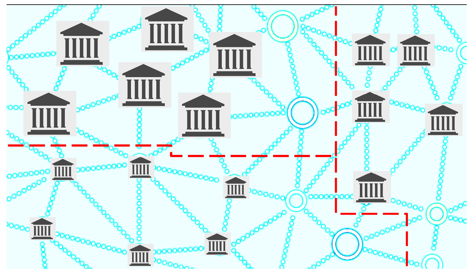
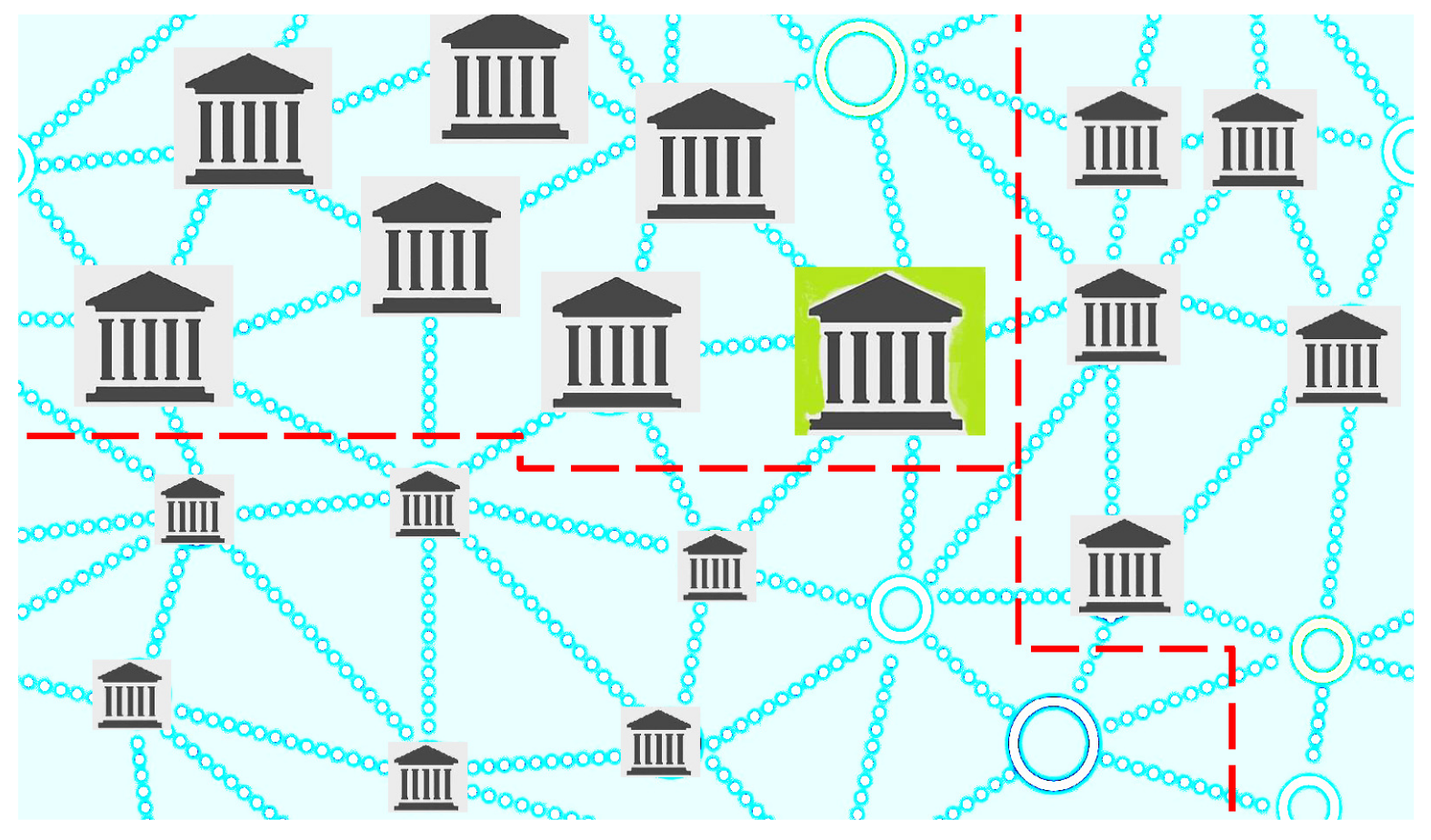
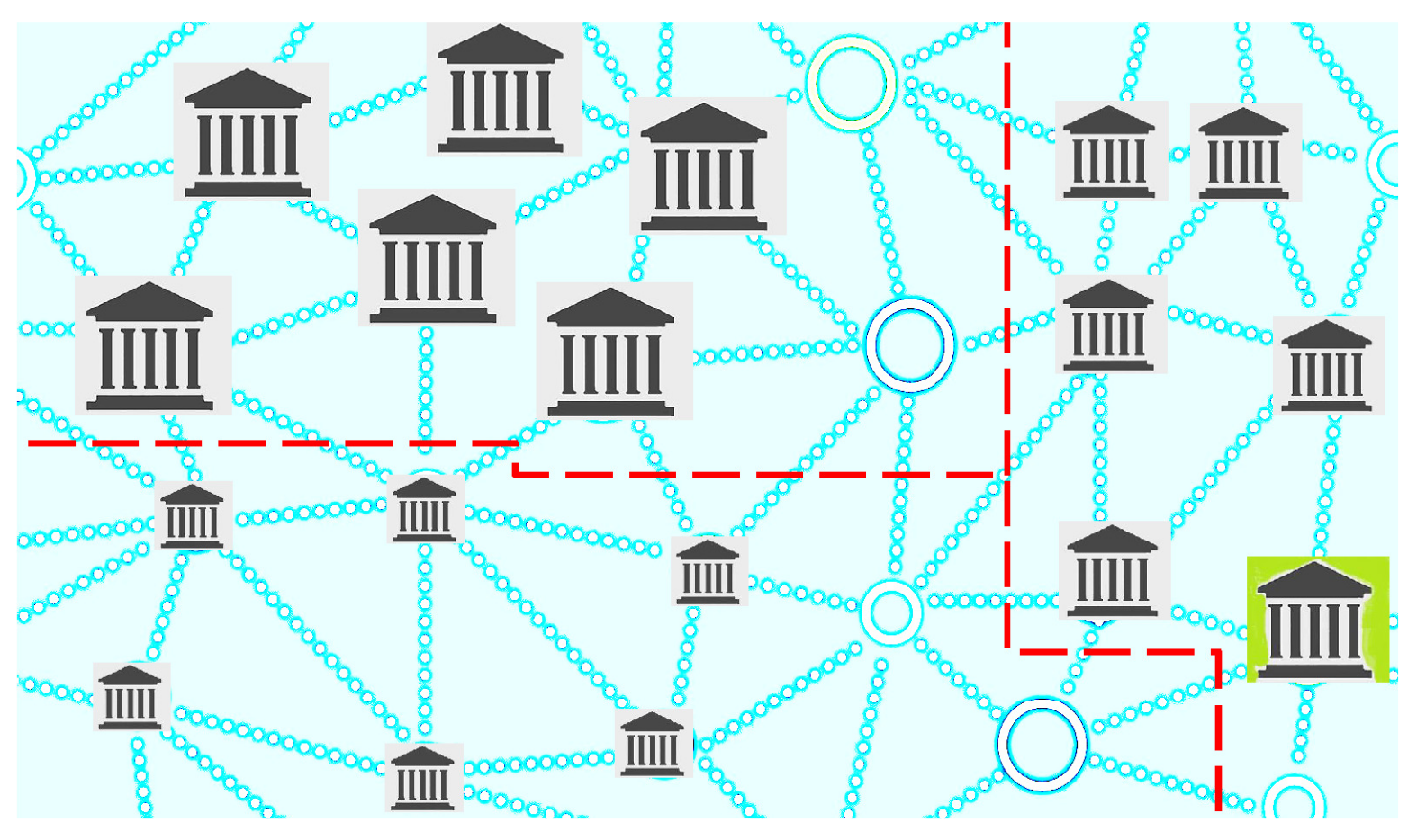
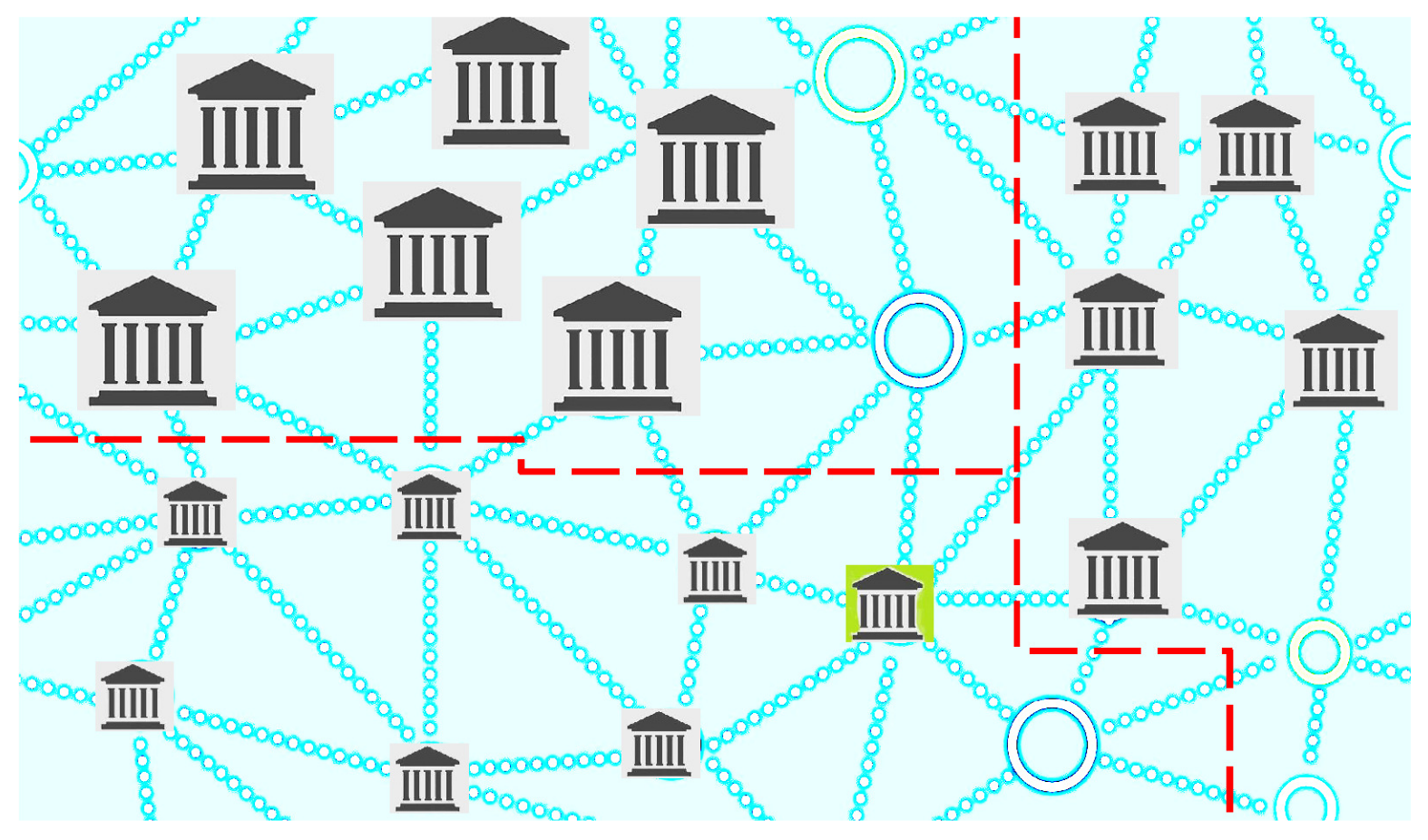
Following the definition of the support network, edges are defined by alternatively defining the neighborhood of a branch. This is formed by those branches which are nearby branches, $N\left(b_i\right)=\{b_j\in BN\mathrm{such}\mathrm{that}d(b_i,b_j)\le k\}$, where “nearby” is understood to mean that there are great similarities in the features related to branches’ cash holdings: following the branch managers’ criteria, this is equivalent to having the same size. As a result, there is an edge linking two branches if and only if they have the same size. Moreover, cliques in the branch network $BN$ are communities of branches with the same size. For instance, cliques in $BN$ may be $C^l$, $C^m$ or $C^s$, representing the clique of branches with a large size, a medium size and a small size, respectively, as shown in Figure 1, Figure 2, Figure 3 and Figure 4.

Remark 4.

Each selection of the random variable (which is stated according to the selected criterion for redesigning) leads to cliques representing different communities of branches. Thus, in a natural way, the original network ($BN$) is granulated depending on the selected criterion.

Thus, the decision making model can now be applied:

• The universal network $(X_v,N_v)$ might be divided into its own cliques $C^i(X_v,N_v)$ depending on the different possibilities for locating a new branch $b^{*}$.
• The new branch $b^{*}$ is added to the above network:

  $$C_{v^{*}}^i(X_v,N_v)=C^i(X_v,N_v)\cup \left\{v^{*}\right\}.$$
• According to Lemma 1, the joint distributions of the sub-networks

  $${\left\{P\left[C_{v^{*}}^i(X_v,N_v)\right]\right\}}_i$$
• may be computed, thereby allowing comparisons between these numerical scores. When more than one output is obtained, the most suitable output is selected according to the given criteria.

Additionally, the BBN is an MRF with respect to branch cash holdings, as shown in the next theorem:

Theorem 2.

Branch network $\{C{H}_b,b\in BN\}$ is a MRF.

Proof. 

We show here that $BN$ is an MRF by proving the corresponding Markov requirement:

$$P[C{H}_b=c_b|C{H}_{BN-\left\{b\right\}}=c_{BN-\left\{b\right\}}]=P[C{H}_b=c_b|C{H}_{N\left(B\right)}=c_{N\left(b\right)}].$$

The result follows from the choice of the features considered. □

According to the Hammersley–Clifford theorem, we may prove the following result:

Corollary 1.

The joint distribution function of the branch network’s cash holdings $CH=\{C{H}_b,b\in BN\}$ $P\left[CH\right)$ is of the form

$$P\left[CH\right)=\frac{1}{Z}\prod _{c\in C}{\varphi }_c\left(C{H}_C\right)=\frac{1}{Z}\prod _{c\in C}{e}^{{\displaystyle \frac{-1}{T}}{V}_c\left(C{H}_C\right)}=\frac{1}{Z}{e}^{{\displaystyle \frac{-1}{T}}{\sum }_{c\in C}{V}_c\left(C{H}_C\right)},$$

where ${\varphi }_c$ are clique potentials and $V_c$ denote energy functions.

Note that Theorem 2 also allows us to specify the weight w of the cliques $C^i$ (see Hao et al., 2018) by computing the ratio between the joint distribution of the clique as MRFs and the joint distribution of the network support, as follows:

$$w_{C^i}={\displaystyle \frac{P\left[\right\{CH,b\in BN\left\}\right]}{P\left[\{CH,b\in C^i\}\right]}}$$

through a selected realization (the mean value of the random variable in a given time interval, for instance) of these random variables (the same for both).

6. Case Study for Non-Physical Networks: Group Decision Making

This section demonstrates the application of the proposed universal decision-making model to the framework of Qualitative Reasoning (QR) as part of an AI approach that analyzes human reasoning with incomplete information. Specifically, an application to reach consensus in Group Decision Making (GDM) problems is provided. Actually, the application to consensus presented in this paper produces a model that is able to measure the consensus within a committee without the need for a moderator (Section 6.1). Further, the theoretical model applied to this context may be used in order to measure the impact of changes in opinions when reaching consensus (Section 6.2).

Group decision making is the process of multiple individuals making decisions by acting collectively, analyzing problems and assessing alternative courses of action in order to select a solution (see the papers [21,22,23,24] for further details). This resembles the general description of our decision-making model (see the Introduction) as a process that would allow the evaluation of the future performance of the network in different scenarios to design the future network structure.

There are several contingencies that define group decision making: the number and nature of people involved, the target of the decision-making groups—either formal (formally designated and charged with a specific task) or informal—and the process used to reach decisions—unstructured or structured …. Due to the global nature of the universal decision-making model, the process described here will be valid for group decision making of any kind. A typical group decision making problem can be formally defined by a set of experts E and a set of alternatives A. Thus, the group decision making problem consists of sorting A using some preferences values provided by the experts. In general, to solve a group decision making problem, the following steps need to be taken:

• The definition of the DMP (decision making process), which includes the descriptions of alternatives and a list of experts, $E=\{e_1,\dots ,e_n\}$;
• Outlining the alternatives, $A=\{a_1,\dots ,a_m\}$;
• Extracting individual preferences: for each participant, a specific preference value is assigned, $P^{e_k},k\in \{1,\dots ,n\}$;
• Calculating the aggregation of collective preferences;
• Ranking alternatives (sorted using the collective preference values);
• Calculating consensus values: the level of consensus reached allows the determination of whether participants in the network community reach a common opinion or not.

The preferences are considered to be fuzzy preference relations in which the preference matrix is additive reciprocal. To this regard, recall that a fuzzy preference relation P on a set of alternatives A is defined as a fuzzy set on the product set $A\times A$, which is identified with a membership function ${\mu }_P:A\times A\to [0,1]$, usually represented by the a matrix $P=\left(pij\right)$, where $p_{ij}={\mu }_P(a_i,a_j)$ is interpreted as the preference degree of the alternative $a_i$ over $a_j$ (for instance, $p_{ij}=1/2$ indicates indifference between $a_i$ and $a_j$, $p_{ij}=1$ indicates that $a_i$ is absolutely preferred to $a_j$ and $p_{ij}>1/2$ indicates that $a_i$ is preferred to $a_j$). As mentioned, it is assumed that the preference matrix, P, is additive reciprocal; i.e., $p_{ij}+p_{ji}=1,\forall i,j\in \{1,\dots ,n\}.$ Reciprocal multiplicative preference relations ($p_{ij}·p_{ji}=1$) could be considered instead (where the equivalence between reciprocal multiplicative preference relations with values in the interval range [1/9, 9] and reciprocal fuzzy preference relations with values in the range [0, 1]) are stated).

For the purposes of applying our universal decision making model, the support network must be defined first. Thus, let us consider the group decision making problem as a network in which each node is represented by an expert $e_k,k=1,\dots ,n$. As the random variable X must be selected according to the goal of reaching consensus, the list of individual fuzzy preferences of each expert over the set of alternatives shall be considered: $X=P=\left(\mathrm{individual}\mathrm{fuzzy}\mathrm{preferences}\right).$ That is, any expert $e_k$ (i.e., any node in the GDM) is identified with the corresponding node of the support network, with the random variable-in-a-site of $P^{e_k}={\left(p_{ij}^{e_k}\right)}^t,k=1,\dots ,n,$ in such a way that any expert $e_k$ is identified with their list of preferences $P^{e_k}$. Note that, using the reciprocity condition, $p_{ji}=1-p_{ij}$, the resulting pairwise comparisons (sometimes structured in a matrix shape) may be gathered into a vector of individual preferences. Following the steps provided before, edges in the support network are defined by alternatively defining the neighborhhood of an expert. To this end, apart from the Euclidean distance, many other definitions in the GDM context (Manhatan, Cosine) may be taken. For further details, see [8] for instance.

Furthermore, as mentioned, the realization of the random variable $P^{e_k}$ may be freely selected. In this context, this can be simply considered as the scores (i.e., the numerical preferences) provided by the experts. Once the support network has been stated, some of its properties should apply: the neighborhood of an expert is composed of those experts with the closest preferences. Moreover, a clique C is a community of experts with a high degree of similarity regarding their preferences with respect to the discussion topic (closest preferences, where the degree of similarity may vary depending on the clique). Importantly, let it be noted that the degree of similarity between preferences is measured by means of the selected distance (as stated in Definition 1), where this distance may be freely selected as necessary.

6.1. The Universal Decision-Making Model used to Measure Consensus

We now show the use of the decision-making model to derive a model that is capable of measuring the consensus within a committee without the use of a moderator. For this, recall that a probability distribution may be associated to each of these cliques (either the original cliques or the original ones plus one more expert) and provides the likelihood of the preferences (as a random variable) of the whole clique in such a way that it enables comparisons between cliques (or cliques plus one more expert).

The process of reaching consensus may be divided into three stages:

• The counting process, which consists of calculating the number of participants who have selected each preference value for each alternative pair.
• The coincidence process, the main goal of which is to aggregate the distances between individual preferences. Thus, the objective is twofold: on the one hand, to find similarities between preferences by computing the distance between them—this is called the LCR process, which consists of finding a common label for each of the groups containing the most similar preferences; on the other hand, to compute the numbers of experts who integrate each of the previous labeled groups.
• The computing process: If D denotes the set of decisions, the calculation of some mean value decision schema of D should imply the selection either of an algebraic consensus (i.e., a mapping $D\times D\to D$) or a topological consensus (i.e., a mapping $D\times D\to L$ for some lattice complete L). An example of algebraic consensus is the (L)OWA ((Label) Ordered Weighted Averaging) operator.

Let it be noted that our approach automatically carries out steps two and three: on the one hand, for the coincidence process, our model aggregates the individual preferences by computing the cliques of the universal network (consisting of those people whose preferences present a high degree of similarity with respect to the distance chosen for this task). On the other hand, for the computing process, the distribution functions corresponding to cliques (viewed as a score attached to each clique) allow us to find the consensus level by simply comparing the scores and selecting the highest one. Many other levels of consensus can be considered. For instance, the level of consensus may be defined as the following ratio:

$${\displaystyle \frac{{\displaystyle \sum _{C_k\mathrm{is}\mathrm{a}\mathrm{clique}}}P[\left\{P^{e_k}\right|e_k\in C_k]}{{\displaystyle \prod _{C_k\mathrm{is}\mathrm{a}\mathrm{clique}}}P[\left\{P^{e_k}\right|e_k\in C_k]}}.$$

The main advantage of this proposal is that different levels of precision can be simultaneously considered without the presence of a moderator as well as many other functions (as shown in the next subsection) that may be executed in parallel.

6.2. The Universal Decision-Making Model to Assess the Impact of Changes in Opinions

The proposed model can evaluate either the impact of a new expert’s entry in the network or the impact of changes of the clique of an existing expert. In the context of GDM, this means that the model may consider the impact of experts’ changing preferences. This could be used to reach consensus when it has not been reached after some attempts have been made.

Based on the standard notion of herd behavior (herding refers to an alignment of behaviors of individuals in a group through local interactions among them), the main result is as follows:

Theorem 3.

Assuming that there is no herd behavior (and no mimetic contagion in consequence), the group decision making (GDM) problem is a Markov random field.

Proof. 

Let $X_{v_i},X_{v_j}$ be two random variables in the same neighborhood. Thus, their distance in terms of similarity with regard to the selected features is as small as desired (as it is the benchmark k). Thus, their marginal distributions are equal, $P\left[X_{v_i}\right]=P\left[X_{v_j}\right]$, and so the corresponding conditional distributions are obtained by the Bayes’ theorem: $P\left[X_{v_i}\right|X_{v_j}]=P\left[X_{v_j}\right|X_{v_i}].$

As a consequence, an opinion depends on those of the cliques with maximum likelihood. Moreover, the assumption of no herd behavior ensures that there will not be any mimetic contagion to modify the collective learning, excepting the nearest opinions (i.e., from the neighborhood of an expert). This means that the Markov property holds: $P[P^{e_k}=p_k|P^{GDM-\left\{e_k\right\}}=p_{GDM-\left\{e_k\right\}}]=P[P^{e_k}=p_k|P^{N\left(e_k\right)}=p_{N\left(e_k\right)}].$ □

Similar to the branch network case, the previous theorem provides extra information that allows us to assign a weight $w_{C^i}$ to the ith-clique by computing the ratio between the joint distribution of the clique as an MRF and the joint distribution of the network support.

Moreover, based on primary notions on collective learning through mimetic contagion, a sketch of a procedure to change opinions in a GDM in case consensus has not been reached may be provided. From the perspective of economic behavior and sociological theories about the interactions and collective dynamics of opinion, one effective way to produce changes in opinion (from opinion A to opinion B) is to “surround” an individual with opinion A by people with opinion B.

In GDM, that would mean moving an expert from their own clique—of opinion A—to another clique: changes in the projects/teams/departments of an employee within a company should provide a new framework for them to be “surrounded” by new opinions. In that case, the proposed universal decision-making model allows the comparison of all the possibilities of change through the corresponding probability distribution whose outputs are the likelihood of the new preferences, expressed by numerical values (see Section 5, step 3 in the model). Thus, the comparison of these outputs allows decisions to be made.

7. Sensitive Study

The previous theorem 1 shows that the joint probability distribution of an MRF is presented in terms of cliques C as

$$P\left[X\right]=\frac{1}{Z}exp\left[-\sum _{C\in \mathcal{C}}f\left(C\right)\right].$$

It is worthy of mention that the comments on this theorem state that the form of function f on clique C (called the energy function) strongly determines the performance of the whole probability distribution in such a way that it is highly advisable to carry out sensitivity tests in order to determine which best represent each particular situation. By and large, function f on clique C may be arbitrarily selected as long as it meets the energy constraint: if the features in a clique match the features in a given template, the energy function decreases; otherwise, it increases. Thus, the general procedure for defining function f on clique C consists of considering it as $f\left(C\right)=1-\lambda \left(C\right)$, where $\lambda$ is an assessment of the similarities between the features of the clique and those of a given template, which may be taken as a distance. Some examples of energy functions $f\left(C\right)$ are $exp\left(c+{\sum }_i{w}_i{f}_i\left(X_{C_i}\right)\right)(\log \mathrm{linear})\mathrm{or}{\displaystyle \frac{{(X_{C_i}-{\mu }_i)}^2}{{\sigma }_i^2}}\left(\mathrm{Gaussian}\right),$ where ${\mu }_i$ and ${\sigma }_i^2$ are the mean and the variance, respectively. Let us consider the Gaussian energy functions in the particular context of the $GDM$, with $P^e$ denoting the preference of an expert e. Following Theorem 3, the GDM process is an MRF. Let us assume that the GMD is granulated into n cliques, $C_k,k=1,\dots ,n$, with each of them containing experts with similar preferences $P^{e_k}$ between them, $P^{e_k},e_k\in C_k$. Then, since the joint probability distribution is $P\left[P^e\right]=\frac{1}{Z}{e}^{-{\sum }_{i=1}^n{\displaystyle \frac{{(P^{e_i}-\mu )}^2}{{\sigma }_i^2}}},$ the probability of GMD obtaining a concrete preference $p^{e_i}=P_{C_i}^e\left(e_i\right)$ may be simply computed as $P[P^e=p^{e_i}]=\frac{1}{Z}{e}^{-{\sum }_{i=1}^n{\displaystyle \frac{{(p^{e_i}-\mu )}^2}{{\sigma }_i^2}}}$, and a similar approach can be taken to compute $P[P^e\le p^{e_i}]$ or $[P^e>p^{e_i}]$.

8. Conclusions

The performance of any network-based system can be improved by an efficient and reliable re-distribution. Dealing with redesigning involves both managing and anticipating the changes. This paper presents a decision-making model that can be used in order to design the future network structure of either physical or non-physical networks. This works on the basis that it allows the evaluation of the future performance of the network in different scenarios, thereby anticipating future needs. As for managing redesigning, our approach benefits from an easy-to handle application performance as it is based on joint probabilistic distributions (working independently) that measure the likelihood of success of any alternative scenarios. If multiple criteria for redesigning are needed, the methodology may be executed in parallel, thereby enhancing the decision-making capabilities of the model. Regarding the potential applications of our model, it has been shown in game theory, for instance [25], that every correlated equilibrium of every graphical game is a Markov random field. In this sense, similar models have been proposed in recent works to solve the problem of opponent state modeling in RTS games (StarCraft) (see [26]), contributing the benefit of giving players an extra dimension with which to compete against the AI or for social media spam detection on Twitter (see [27]).

Moreover, one of the advantages of our approach is that it is geographical constraint-free, which makes it suitable for cross-border enterprises as well as expands its range of potential applications. Apart from physical networks, group decision making, social networks and all groups of users that make decisions together (ranking and recommendation systems, online prediction markets) can now be included in the application scope.

Regarding future lines of research, alternative fuzzy versions of our DMM that incorporate the use and development of linguistic information are under consideration (see [28]). Furthermore, although the case of multiple criteria is possible now in our model, new proposals for decision-making models with multiple criteria based on incomplete information should be considered (see [29]).