An Optimized Triggering Algorithm for Event-Triggered Control of Networked Control Systems

Abstract

This paper presents an optimized algorithm for event-triggered control (ETC) of networked control systems (NCS). Initially, the traditional backstepping controller is designed for a generalized nonlinear plant in strict-feedback form that is subsequently extended to the ETC. In the NCS, the controller and the plant communicate with each other using a communication network. In order to minimize the bandwidth required, the number of samples to be sent over the communication channel should be reduced. This can be achieved using the non-uniform sampling of data. However, the implementation of non-uniform sampling without a proper event triggering rule might lead the closed-loop system towards instability. Therefore, an optimized event triggering algorithm has been designed such that the system states are always forced to remain in stable trajectory. Additionally, the effect of ETC on the stability of backstepping control has been analyzed using the Lyapunov stability theory. Two case studies on an inverted pendulum system and single-link robot system have been carried out to demonstrate the effectiveness of the proposed ETC in terms of system states, control effort and inter-event execution time.

1. Introduction

In recent years, event-triggered control (ETC) has become a prominent topic of research due to the benefits offered by it as compared to the networked control system (NCS). The analog-to-digital (A/D) and digital-to-analog (D/A) conversion of the plant data is essential in the NCS to make the plant and controller signals compatible with the communication channel. This further needs the sampling and hold circuit for the plant data. Periodic sampling utilizes a fixed bandwidth on the communication channel and was preferred in the past for implementing the NCS. This, however, increases the cost of the system. In several control applications (e.g., chemical processes which take a longer time to settle), it is not needed to send the output data of the plant to the controller at fixed time intervals. The time interval between the samples can be varied (also called the aperiodic sampling of data) depending on the specific system events. Whenever the quantization error reaches beyond an acceptable limit, an event is triggered to sample the output data. Thereafter, a new control command is computed and the plant control input is updated. This control command is kept on hold until a new event is triggered and this process repeats. In this manner, the number of samples can be reduced significantly without disturbing the desired plant performance.

1.1. Literature Review

A plethora of research works have been published on this topic. Some of the original ETC studies were focused on the PID controller, which due to its basic configuration is still one of the commonly used controllers in industrial applications. In [1], a simple event-based PID control scheme was proposed, where the aim was to control the level of the upper or lower tank with the pump signal as the control signal. Another event-based PID controller was proposed in [2], where the objective was to control the angular velocity of a DC-motor. However, the emphasis has moved in the past 10 years toward ETC for optimized, adaptive and nonlinear controllers. That is because of the nonlinear nature of the control schemes. The nonlinear system has to be linearized to construct the linear controllers, which may lead to optimum performance. In [3], a critic neural network (NN) was used to approximate the cost and an actor neural network was used to approximate the optimal event-triggered controller. The controller stability was ensured by Lyapunov stability analysis. Again in [4], an approximation-based event-triggered control of multi-input multi-output uncertain nonlinear continuous-time systems was presented that included weight update law for aperiodic tuning of the NN weights at triggered instants to reduce the computation. In [5], the effects of bounded disturbances on the integral-based event-triggered control systems with observer-based output feedbacks were studied. In [6], a robust adaptive fuzzy control for a class of uncertain nonlinear systems via an event-triggered control strategy to reduce communication burden had been proposed, and results were demonstrated on a robot manipulator. In [7], the event-triggered function under the conditions of limited network bandwidth resources and the incomplete observability of the state of the system was considered. Then, denial-of-service (DoS) attacks that occur on the network transmission channel were applied using observer-based event-triggered control.

It is well known that the ETC can provide efficient utilization of resources by decreasing the sample size, which in turn reduces the overall bandwidth requirement of the communication channel. However, the ETC technique may lead the system towards instability if it is not driven by a suitable event triggering algorithm. Many triggering algorithms for the ETC scheme have been proposed in recent times, with impractical applications in wireless networks [8], robotics [9] and power systems [10].

A detailed review of these earlier techniques in the area of ETC has been published in [11], whereas a detailed review of several control techniques developed till recently could be found in [12]. Recently, ETC schemes that use a sliding mode controller (SMC) have been proposed for linear and nonlinear systems. In [13], a robust stabilization of a linear time-invariant system using an SMC with the self-triggering strategy was proposed. The self-triggering technique does not require additional dedicated hardware for continuous state measurement to determine the next possible triggering instant. In [14], robust stabilization for a class of nonlinear systems subject to external disturbances using an ETC-based SMC was proposed. Similarly, in [15], a global event-triggering realization of an SMC was proposed for linear systems under the effect of uncertainties. While the ETC–SMC scheme reduces the control updates considerably, the SMC itself is plagued by chattering.

The ETC schemes other than SMC have also been demonstrated in many studies [16,17,18,19,20,21,22]. In [16], it was explained how self-triggering rules could be deduced from the developed event-triggered strategies. The stabilization of nonlinear systems using event-triggered output feedback controllers was presented by [17], which guarantees an asymptotic stability property and enforces a minimum amount of time between two consecutive transmission instants. In [18], an event-driven tracking control algorithm for a marine vessel, based on the backstepping method, was proposed. In [19], adaptive event-triggered control of nonlinear continuous time systems in the strict feedback form is presented. An adaptive model and an associated event-triggered controller were designed by using the backstepping method. The backstepping method proposed by [18] was limited to marine vessels only, whereas [19] focused upon a neural network-based adaptive event-triggered backstepping controller scheme. In [20], both the parameter estimator and the controller were aperiodically updated only at the event-sampled instants, and an adaptive event sampling condition was designed to determine the event sampling instants. The system in [20] was not considered in a very generalized form of nonlinear system in strict-feedback form. An event-triggered nonlinear control based on the backstepping controller of an oscillating water column ocean wave energy plant was proposed by [21,22]. The second order nonlinear plant dynamics were considered in [21], whereas several wave energy plants were considered in [22] for forming an array of ocean energy plants, which also included an NCS.

In recent years, there has been a main focus on nonlinear systems while designing ETC [23,24,25,26,27,28,29,30,31,32]. In [23], a user-adjustable event-triggered mechanism based on the sampled state vectors and backstepping techniques for a nonlinear system was developed to determine the sampling state instants using the negative definite property of the derivatives of Lyapunov functions. In [24], event-triggered adaptive control for a class of nonlinear systems in Brunovsky form was considered. In [25], the considered nonlinear system contained not only unknown system parameters, but the nonlinear functions with no requirement to be globally Lipschitz. It was claimed to be in contrast to most of the existing results in the area. In [26], time-varying external disturbances were considered apart from the conditions given in [25], and the ETC was designed which can dynamically compensate for both errors caused by disturbances and the sampled-data implementation of the controller. In [27], the feedback linearization approach was applied to design the ETC for a nonlinear system, whereas [28] considered both the disturbances and transmission delays while designing the ETC scheme. In [29], an ETC scheme with nonlinear model predictive control was designed for an unmanned aerial vehicle. In [30], a self-learning robust ETC scheme was proposed for nonlinear interconnected systems subject to uncertainty. A fuzzy logic-based ETC–SMC was designed for a nonlinear system in [31]. In [32], a fractional order system was controlled using a fractional order controller where the controller interacted using a communication network. The above-mentioned studies have maintained the closed-loop stability of the systems but not considered the optimized event triggering parameters. The non-optimized event triggering parameters affect the closed-loop performance of the system significantly. Additionally, some classes of nonlinear systems have been considered in the studies discussed above. Most of the systems considered have restricted the system order. Hence, an optimized event-triggered control for a generalized nonlinear system is to be designed to accommodate different practical nonlinear systems. It is also to be noted that the backstepping controller is free from the chattering problem which predominantly exists in the SMC [20,21,22].

1.2. Main Contributions

Based on the literature review, this paper contributes two novel concepts to the NCS: (i) the design of an ETC scheme for an NCS wherein the NCS consists of a nth order nonlinear plant (or generalized nonlinear system) in strict-feedback form, a backstepping controller, and a communication channel; and (ii) the selection of the optimum value of event triggering parameter $\alpha$ to attain the best possible outcome of ETC as compared to the conventional approach. Firstly, a backstepping controller has been designed using the conventional approach and then it has been extended to ETC. The closed-loop asymptotic stability of the system is ensured while deriving the triggering rule for the backstepping controller. Next, the particle swarm optimization (PSO) technique [33] has been applied to obtain the optimum value of event triggering parameter $\alpha$. In this regard, a fitness function consisting of error in system states and the number of triggering pulses are defined, wherein $\alpha$ has been chosen as an unknown parameter.

Two case studies on the inverted pendulum system [34] and a single-link robot system [20] are considered for demonstration purposes. Simulations are performed in MATLAB software for these two nonlinear systems in strict-feedback form. Additionally, the analysis of a control system with different values and optimum values of event triggering parameter $\alpha$ is presented to show the effectiveness of the proposed ETC scheme.

The remaining sections are arranged in the following order: Section 2 gives an overview of the ETC scheme for the NCS and defines the control problem. In Section 3, the ETC using a backstepping controller has been developed. Section 4 discusses the simulation results, followed by the conclusion in Section 5.

2. Description of ETC for NCS and Control Problem Statement

The block diagram of an NCS with a backstepping controller, nth order nonlinear plant, communication network, and event triggering section is shown in Figure 1. The output of the plant first passes through a triggering section where non-uniform sampling is performed. Next, it is sent to the backstepping controller using the communication channel and a control command is computed. The control command then passes through the communication channel. It is further processed using zero-order-hold (ZOH) and given to the plant. It is obvious that there will be a quantization error in system states due to the sampling and hold of plant output data. This quantization error is taken as the criterion for event triggering, which then governs the sample and hold switch function.

Consider a generalized nth order nonlinear system in strict-feedback form as:

$$\begin{array}{c}{\dot{x}}_i=f_i\left(x_1,x_2,\dots ,x_i\right)+g_i\left(x_1,x_2,\dots ,x_i\right)·x_{i+1}\\ {\dot{x}}_n=f_n\left(x_1,x_2,\dots ,x_n\right)+g_n\left(x_1,x_2,\dots ,x_n\right)·u\end{array}\}$$

(1)

where $n\ge 2$, x_i corresponds to system states and i = 1, 2, …, n − 1; u is the control input to the plant. The $f_i\left(x_1,x_2,\dots ,x_i\right)$, $f_n\left(x_1,x_2,\dots ,x_n\right)$ and $g_i\left(x_1,x_2,\dots ,x_i\right)$, …, $g_n\left(x_1,x_2,\dots ,x_n\right)$ are the nonlinear functions dependent upon the system states. The control input u(t) is represented by u in the continuous time domain, but with ETC where sample and hold interface is involved, u is represented as u_k, where k represents the kth triggering instant for k = 1, 2, 3, …, ∞.

For simplicity of representation, the system in Equation (1) can be written as:

$$\begin{array}{c}{\dot{x}}_i=f_i+g_i·x_{i+1}\\ {\dot{x}}_n=f_n+g_n·u \end{array}\}$$

(2)

where $g_i\ne 0$; for $i=1, 2,\dots , n$. Here, it is also assumed that the time derivatives of f_i and g_i do exist for all time, t. The system states in the vector form are defined as:

$$X=\left[x_1 x_2 \dots x_n\right]$$

(3)

3. Design of Backstepping Controller and ETC Scheme

3.1. Backstepping Controller Design

Initially, we derive a backstepping control law using the conventional approach and then a triggering rule for implementing ETC is designed. In the backstepping controller, a step by step design method is followed. The error components for system states can be defined as:

$$\begin{array}{c}{\tilde{x}}_i=x_{id}-x_i \\ {\tilde{x}}_{n+1}=x_{\left(n+1\right)d}-u\end{array}\}\mathrm{for}i=1,2,\dots ,n$$

(4)

where x_1d is the reference trajectory for system state x₁ and x_2d, x_3d, …, x_{(n − 1)d}, x_nd are the virtual control inputs for corresponding system states, and:

$$u=x_{\left(n+1\right)d}-{\tilde{x}}_{n+1}$$

(5)

Here, we define the error variable ${\tilde{x}}_{n+1}$ additionally to maintain the uniformity of all the error variables of system states. This can also be called the virtual control input for actual control input u, as given in Equation (5).

The first order derivative of ith error variable ${\tilde{x}}_i$ is given by:

$${\dot{\tilde{x}}}_i={\dot{x}}_{id}-{\dot{x}}_i={\dot{x}}_{id}-f_i-g_i·x_{i+1}$$

(6)

Now, we add and subtract the $g_i.x_{\left(i+1\right)d}$ term into Equation (7) as:

$$\begin{array}{c}{\dot{\tilde{x}}}_i={\dot{x}}_{id}-f_i-g_i·x_{i+1}+g_i·x_{\left(i+1\right)d}-g_i·x_{\left(i+1\right)d}\\ ={\dot{x}}_{id}-f_i+g_i·{\tilde{x}}_{i+1}-g_i·x_{\left(i+1\right)d} \end{array}\}$$

(7)

Define the ith virtual control law $x_{\left(i+1\right)d}$,

$$x_{\left(i+1\right)d}=g_i^{-1}\left[{\dot{x}}_{id}-f_i+k_i·{\tilde{x}}_i\right]$$

(8)

Such that,

$${\dot{\tilde{x}}}_i=-k_i·{\tilde{x}}_i+g_i·{\tilde{x}}_{i+1}$$

(9)

where k_i > 0 for i = 1, 2, …, n.

Next, define the control law as:

$$u=g_n^{-1}\left[{\dot{x}}_{nd}-f_n+k_n·{\tilde{x}}_n\right]+{\left({\varphi }_n\right)}^{-1}\left\{{{\displaystyle \sum }}_{i=1}^{n-1}{\varphi }_i\right\}+\eta {\varphi }_n$$

(10)

where η is a positive constant and η > 0. Additionally, ${\varphi }_i=g_i·{\tilde{x}}_i·{\tilde{x}}_{i+1}$ and ${\varphi }_n=g_n·{\tilde{x}}_n$.

After substituting the $x_{\left(n+1\right)d}$ and $u$ in Equation (5), the error variable ${\tilde{x}}_{n+1}$ can be written as:

$${\tilde{x}}_{n+1}=-{\left({\varphi }_n\right)}^{-1}\left\{{{\displaystyle \sum }}_{i=1}^{n-1}{\varphi }_i\right\}-\eta {\varphi }_n$$

(11)

Theorem 1.

Consider a nonlinear system in strict-feedback form (Equation (2)) and the error dynamics (Equation (9)). Then, the virtual control law (Equation (8)) and backstepping control law (Equation (10)) ensure that all the equilibrium points,${\tilde{x}}_i$for$i=1, 2,\dots , n$, are globally asymptotically stable. Therefore, the closed-loop system states,$x_i$, are bounded.

Proof. 

In order to prove the global asymptotic stability of a nonlinear system in strict-feedback form (Equation (2)) and the error dynamics (Equation (9)), we define a positive definite function $V\left(t\right)$ as a Lyapunov function candidate as follows:

$$V\left(t\right)=\frac{1}{2}{{\displaystyle \sum }}_{i=1}^n{\tilde{x}}_i^2$$

(12)

As per Lyapunov stability theory, if the $V\left(t\right)$ is a positive definite function and its first order derivative $\dot{V}\left(t\right)$ is a negative definite, then ${\tilde{x}}_i$ will be of converging nature and will be globally asymptotically stable. The Lyapunov function candidate in Equation (13) will then become a Lyapunov function. Hereafter, in the next few steps, it will be proved that $\dot{V}\left(t\right)$ is negative definite function.

The first order time derivative of Equation (12) is given as:

$$\dot{V}\left(t\right)={{\displaystyle \sum }}_{i=1}^n{\tilde{x}}_i·{\dot{\tilde{x}}}_i$$

(13)

Substituting Equation (9) into Equation (13) as:

$$\dot{V}\left(t\right)=-{{\displaystyle \sum }}_{i=1}^n{k}_i·{\tilde{x}}_i^2+{{\displaystyle \sum }}_{i=1}^n{g}_i·{\tilde{x}}_i·{\tilde{x}}_{i+1}$$

(14)

$$\Rightarrow \dot{V}\left(t\right)={\dot{V}}_1\left(t\right)+{\dot{V}}_2\left(t\right)$$

(15)

Here, we choose,

$${\dot{V}}_1\left(t\right)=-{{\displaystyle \sum }}_{i=1}^n{k}_i·{\tilde{x}}_i^2\mathrm{for}{k}_i>0$$

(16)

And

$${\dot{V}}_2\left(t\right)={{\displaystyle \sum }}_{i=1}^n{g}_i·{\tilde{x}}_i·{\tilde{x}}_{i+1}$$

(17)

$$\Rightarrow {\dot{V}}_2\left(t\right)={{\displaystyle \sum }}_{i=1}^{n-1}{g}_i·{\tilde{x}}_i·{\tilde{x}}_{i+1}+g_n·{\tilde{x}}_n·{\tilde{x}}_{n+1}$$

(18)

$$\Rightarrow {\dot{V}}_2\left(t\right)={{\displaystyle \sum }}_{i=1}^{n-1}{\varphi }_i+{\varphi }_n·{\tilde{x}}_{n+1}$$

(19)

In Equation (19), substituting the error variable ${\tilde{x}}_{n+1}$ from Equation (11), we then have:

$${\dot{V}}_2\left(t\right)=-\eta {\varphi }_n^2\Rightarrow {\dot{V}}_2\left(t\right)\le 0$$

(20)

where η > 0.

Therefore, after combining the results of Equations (16) and (20) into Equation (15), we have:

$$\dot{V}\left(t\right)=-{{\displaystyle \sum }}_{i=1}^n{k}_i·{\tilde{x}}_i^2-\eta {\varphi }_n^2\le 0$$

(21)

Equation (21) is negative definite and, hence, the Lyapunov function candidate defined in Equation (12) has now become the Lyapunov function and Theorem 1 is proved. □

Remark 1.

Theorem 1 implies that the control law in Equation (10) will result in$\underset{t\to \infty }{\lim }{\tilde{x}}_i\to 0,$for$i=1, 2,\dots , n$. Next, from Equation (4), if$\underset{t\to \infty }{\lim }{\tilde{x}}_i\to 0$then$\underset{t\to \infty }{lim}{x}_i\to x_{id}$, for$i=1, 2,\dots , n$. Hence, it can be concluded that if${\tilde{x}}_i$is globally asymptotically stable around the origin as$t\to \infty$, then$x_i$would be globally asymptotically stable around$x_{id}$as$t\to \infty$. Therefore, as per Theorem 1, the nonlinear system (Equation (2)) would always lead towards global asymptotic stability with the control input defined by Equation (10).

3.2. ETC Scheme with Backstepping Controller

As shown in Figure 1, the nonlinear system state vector, $X\left(t\right)$, is first sent to the sampling block where it is discretized and is represented by $X\left(t_k\right)$. Additionally, the reference variable, $x_{1d}$, is discretized into $x_{1d}\left(t_k\right)$. Then, $X\left(t_k\right)$ and $x_{1d}\left(t_k\right)$ are sent to the controller via the communication channel and the controller output, $u\left(t_k\right)$, which is in discrete form, is calculated. Next, the controller output, $u\left(t_k\right)$, is sent back to the nonlinear system again via the same communication channel, and after passing through the ZOH block, it is converted into continuous form, i.e., $u_k\left(t\right)$. Hence, $u_k\left(t\right)$ given by Equation (23) is not a discrete signal, but it is a continuous signal. However, $u_k\left(t\right)$ would not be exactly similar to the original continuous control signal $u$ (t) due to the quantization error created by the sample and hold circuit. Due to ETC implementation, the system dynamics given by Equation (2) can be rewritten as:

$$\begin{array}{c}{\dot{x}}_i=f_i+g_i·x_{i+1}\\ {\dot{x}}_n=f_n+g_n·u_k \end{array}\}$$

(22)

The designed control law in Equation (10) ensures the asymptotic stability of the closed-loop system in continuous time. Now, in this section, the backstepping control law (in Equation (10)) would be converted into ETC law, which is given as:

$$\begin{array}{c}{u}_k=g_{nk}^{-1}\left[{\dot{x}}_{ndk}-f_{nk}+k_n·{\tilde{x}}_{nk}\right]+{\left({\varphi }_{nk}\right)}^{-1}\left\{{\displaystyle \sum }_{i=1}^{n-1}{\varphi }_{ik}\right\}+\eta {\varphi }_{nk}\\ \end{array}$$

(23)

where $k$ represents the sample number.

Therefore, all time dependent variables in the control law of Equation (10) are replaced by suffix $k$ to represent ETC. Next, the virtual control law from Equation (8) can be recalled as:

$$x_{\left(i+1\right)d}=g_i^{-1}\left[{\dot{x}}_{id}-f_i+k_i·{\tilde{x}}_i\right]\mathrm{for}i=1,2,\dots ,n-1$$

(24)

and because of the effect of the ETC implementation, the virtual control law can be written as:

$$x_{\left(n+1\right)dk}=g_{nk}^{-1}\left[{\dot{x}}_{ndk}-f_{nk}+k_n·{\tilde{x}}_{nk}\right]$$

(25)

The error dynamics of Equation (9) due to ETC implementation can now be rewritten as:

$$\begin{array}{c}{\dot{\tilde{x}}}_i=-k_i·{\tilde{x}}_i+g_i·{\tilde{x}}_{i+1} \\ {\dot{\tilde{x}}}_n=-k_n·{\tilde{x}}_n+g_n·{\tilde{x}}_{\left(n+1\right)k}\end{array}\}\mathrm{for}i=1,2,\dots ,n-1$$

(26)

Additionally, Equation (11), due to ETC implementation, can be written as:

$${\tilde{x}}_{\left(n+1\right)k}=-{\left({\varphi }_{nk}\right)}^{-1}\left\{{{\displaystyle \sum }}_{i=1}^{n-1}{\varphi }_{ik}\right\}-\eta {\varphi }_{nk}$$

(27)

The virtual control law in Equation (27) creates a quantization error in the system states and subsequently affects its stability. Therefore, we define a quantization error due to ETC as follows:

$${\xi }_i={\varphi }_i-\gamma {\varphi }_{ik}\mathrm{for}i=1,2,\dots ,n-1$$

(28)

where $\gamma ={\varphi }_n{\varphi }_{nk}^{-1}$.

The ${\xi }_i$ in Equation (28) is the quantization error created during the sample and hold process of the closed-loop system. Due to non-uniform sampling, there might be an undesired time interval between two sampling instants. It may lead the closed-loop system towards instability unless there is a mechanism to limit the quantization error within the permissible range of operation. Hence, we place an upper bound on ${{\displaystyle \sum }}_{i=1}^{n-1}\left|{\xi }_i\right|$ such that,

$${{\displaystyle \sum }}_{i=1}^{n-1}\left|{\xi }_i\right|={{\displaystyle \sum }}_{i=1}^{n-1}\left|{\varphi }_i-\gamma {\varphi }_{ik}\right|\le \alpha ,\forall t\ge 0$$

(29)

or,

$${\left({{\displaystyle \sum }}_{i=1}^{n-1}\left|{\xi }_i\right|\right)}_{max}=\alpha$$

(30)

where the upper bound α is a non-zero positive constant and, hence, we refer to it as a triggering parameter.

Next, we also place a lower bound on ${\varphi }_n{\varphi }_{nk}$ such that,

$${\varphi }_n{\varphi }_{nk}\ge \frac{\alpha }{\eta },\forall t\ge 0$$

(31)

Remark 2.

During the implementation of the event triggering algorithm, if${\varphi }_n{\varphi }_{nk}<\alpha /\eta$then the virtual control law (Equations (24) and (25) and backstepping control law (Equation (23)) would fail to ensure the semiglobal asymptotic stability of the error variables, ${\tilde{x}}_i$and closed-loop system states,$x_i$for$i=1, 2,\dots , n$. It is therefore necessary to maintain${\varphi }_n{\varphi }_{nk}\ge \alpha /\eta , \forall t\ge 0$. The region of attraction exists as long as the conditions: (i)${{\displaystyle \sum }}_{i=1}^{n-1}\left|{\xi }_i\right|\le \alpha , \forall t\ge 0$and (ii)${\varphi }_n{\varphi }_{nk}\ge \alpha /\eta , \forall t\ge 0$, are satisfied.

In order to ensure the stability of the closed-loop system with ETC, the upper boundedness on ${{\displaystyle \sum }}_{i=1}^{n-1}{\xi }_i$ as defined by Equations (29) and (30) and the necessary condition, ${\varphi }_n{\varphi }_{nk}\ge \alpha /\eta \forall t\ge 0$, must be maintained. Therefore, a triggering algorithm has been designed and is described in Algorithm 1. If the condition given in Algorithm 1 is satisfied, then the system will trigger an event which will send the new sample to the controller. The control command will then be computed and sent back to the nonlinear system after passing through the communication network and ZOH block. If the condition given in Algorithm 1 is not satisfied, then the previous control command will remain in the nonlinear system input.

Algorithm 1. Event Triggering Algorithm

if ${{\displaystyle \sum }}_{i=1}^{n-1}\left|{\xi }_i\right|\ge \alpha$or${\varphi }_n{\varphi }_{nk}\le \alpha /\eta$

(i) an event is triggered ($y_{trig}\left(t\right)=1$) and

(ii) control command is updated

else

(i) no event triggering ($y_{trig}\left(t\right)=0$) and

(ii) control command is on hold at its previous value

end

Next, the stability analysis of the closed-loop system with ETC law is again performed using the Lyapunov stability theory. In this regard, Theorem 2 is described next, followed by its proof.

Theorem 2.

Consider a nonlinear system in strict-feedback form (Equation (2)), and the error dynamics due to ETC (Equation (26)). Then, the virtual control law (Equations (24) and (25), backstepping control law (Equation (23)) and event triggering algorithm (Algorithm 1) ensure that all the equilibrium points, ${\tilde{x}}_i$for$i=1, 2,\dots , n$, are semiglobally asymptotically stable with region of attraction-${{\displaystyle \sum }}_{i=1}^{n-1}\left|{\xi }_i\right|\le \alpha$and${\varphi }_n{\varphi }_{nk}\ge \alpha /\eta$. Therefore, the closed-loop system states,$x_i$, are bounded.

Proof. 

It is again required to revisit the Lyapunov function candidate (Equation (12)) to analyze the effect of non-uniform sampling and ETC implementation on the system stability. The derivative of the Lyapunov function candidate from Equation (13) is recalled here as:

$$\dot{V}\left(t\right)={{\displaystyle \sum }}_{i=1}^n{\tilde{x}}_i.{\dot{\tilde{x}}}_i={{\displaystyle \sum }}_{i=1}^{n-1}{\tilde{x}}_i·{\dot{\tilde{x}}}_i+{\tilde{x}}_n·{\dot{\tilde{x}}}_n$$

(32)

Substituting Equation (26) into Equation (32), we have:

$$\dot{V}\left(t\right)=-{{\displaystyle \sum }}_{i=1}^n{k}_i·{\tilde{x}}_i^2+{{\displaystyle \sum }}_{i=1}^{n-1}{\varphi }_i+{\varphi }_n·{\tilde{x}}_{\left(n+1\right)k}$$

(33)

Here, Equation (33) can be divided into two parts as ${\dot{V}}_1\left(t\right)$ and ${\dot{V}}_2\left(t\right)$. ${\dot{V}}_1\left(t\right)$ is independent of ETC law and reduces to Equation (16). ${\dot{V}}_2\left(t\right)$ is dependent on ${\tilde{x}}_{\left(n+1\right)k}$ and can be written as:

$${\dot{V}}_2\left(t\right)={{\displaystyle \sum }}_{i=1}^{n-1}{\varphi }_i+{\varphi }_n·{\tilde{x}}_{\left(n+1\right)k}$$

(34)

Putting the expression of ${\tilde{x}}_{\left(n+1\right)k}$ from Equation (27) into Equation (34), we have:

$${\dot{V}}_2\left(t\right)={{\displaystyle \sum }}_{i=1}^{n-1}{\varphi }_i+{\varphi }_n·\left[-{\left({\varphi }_{nk}\right)}^{-1}\left\{{{\displaystyle \sum }}_{i=1}^{n-1}{\varphi }_{ik}\right\}-\eta {\varphi }_{nk}\right]$$

(35)

$$\Rightarrow {\dot{V}}_2\left(t\right)=-\eta {\varphi }_n{\varphi }_{nk}+{{\displaystyle \sum }}_{i=1}^{n-1}\left({\varphi }_i-\gamma {\varphi }_{ik}\right)$$

(36)

where $\gamma ={\varphi }_n·{\varphi }_{nk}^{-1}$.

Equation (36) can further be simplified by substituting Equation (28) as:

$${\dot{V}}_2\left(t\right)=-\eta {\varphi }_n{\varphi }_{nk}+{{\displaystyle \sum }}_{i=1}^{n-1}{\xi }_i$$

(37)

While implementing the ETC scheme, two conditions arise due to sampling.

Condition 1. At sampling instants, e.g., at $t=t_k$ and $t=t_{k+1}$, we have:

$${\varphi }_i={\varphi }_{ik}\mathrm{for}i=1,2,\dots ,n$$

(38)

Therefore, Equation (38) implies that:

$${{\displaystyle \sum }}_{i=1}^{n-1}{\xi }_i=0\mathrm{and}\gamma =1$$

(39)

Therefore, Equation (37) reduces to the following form:

$${\dot{V}}_2\left(t\right)=-\eta {\varphi }_n^2\Rightarrow {\dot{V}}_2\left(t\right)\le 0$$

(40)

which is same as Equation (20) and further results in Equation (21), and implies that the system states would always lead towards asymptotic stability.

Condition 2. Between any two consecutive sampling instants, e.g., $t_k<T_k<t_{k+1}$, we have:

$${\varphi }_i\ne {\varphi }_{ik}\mathrm{for}i=1,2,\dots ,n$$

(41)

Therefore, Equation (41) implies that:

$${{\displaystyle \sum }}_{i=1}^{n-1}{\xi }_i\ne 0\mathrm{or}{{\displaystyle \sum }}_{i=1}^{n-1}\left|{\xi }_i\right|>0$$

(42)

and $\gamma \ne 1$.

Next, we can further simplify Equation (37) as:

$${\dot{V}}_2\left(t\right)\le -\eta {\varphi }_n{\varphi }_{nk}+{\left({{\displaystyle \sum }}_{i=1}^{n-1}\left|{\xi }_i\right|\right)}_{max}$$

(43)

Substituting Equation (30) into Equation (43) as:

$${\dot{V}}_2\left(t\right)\le -\eta {\varphi }_n{\varphi }_{nk}+\alpha$$

(44)

$$\Rightarrow {\dot{V}}_2\left(t\right)\le -\eta \left({\varphi }_n{\varphi }_{nk}-\frac{\alpha }{\eta }\right)$$

(45)

Substituting Equation (31) in Equation (45), we get:

$${\dot{V}}_2\left(t\right)\le 0$$

(46)

Now, Equation (46) along with Equation (16) is converted to the following form:

$$\dot{V}\left(t\right)\le -{{\displaystyle \sum }}_{i=1}^n{k}_i·{\tilde{x}}_i^2\le 0$$

(47)

From Equations (40) and (47), it can be concluded that the Lyapunov function candidate defined by Equation (12) is now a Lyapunov function and the closed-loop system with the ETC scheme is semi-globally asymptotically stable. Hence, Theorem 2 is proved for both Condition 1 and Condition 2. □

3.3. Design of Optimized Event Triggering Algorithm

As given in Algorithm 1, it is also very important to choose triggering parameter $\alpha$ very carefully so that both the objectives of attaining desired system performance and of sending a minimum number of samples over the communication network are achieved successfully. A numerical analysis of the need for an optimum value of triggering parameter $\alpha$ is presented in Section 4. In order to optimize $\alpha$, a fitness function consisting of error in system states and the number of triggering pulses is defined wherein $\alpha$ has been chosen as an unknown parameter. This can be seen in Figure 2 wherein the output of the nonlinear system, i.e., $X\left(t\right)$, and the output of the triggering block, i.e., $y_{trig}\left(t\right)$, are given as an input to the fitness function block. The fitness function is given as:

$$J_{fit}\left(t\right)={{\displaystyle \int }}_0^{T_s}\left\{t·\Vert X\left(t\right)\Vert +\left|y_{trig}\left(t\right)\right|\right\}dt$$

(48)

where $\Vert X\left(t\right)\Vert$ is the Euclidean norm, and its mathematical expression is given as:

$$\Vert X\left(t\right)\Vert =\sqrt{x_1^2+x_2^2+\dots +x_n^2}$$

(49)

The $y_{trig}\left(t\right),$ represents the triggering pulses which actually drive the sample and hold circuit. The $y_{trig}$ always toggles between 0 and 1. The $y_{trig}\left(t\right)=1$ means that the switches in AS and ZOH blocks (in Figure 1) are closed, whereas the switches are opened for $y_{trig}\left(t\right)=0$.

$J_{fit}\left(t\right)$ in Equation (48) is the summation of two fitness functions as: (i) integral time norm of system states, i.e., $\Vert X\left(t\right)\Vert$ and (ii) integral absolute of triggering function, i.e., $y_{trig}\left(t\right)$. The reason for multiplying time with $\Vert X\left(t\right)\Vert$ is that in the transient phase of the simulation, the errors in the system state are high, whereas in the steady state stage the errors become very low. Hence, in the final stage of simulation, if the time is multiplied with $\Vert X\left(t\right)\Vert$, then the errors become significant for optimization purposes. However, the time is not multiplied to $\left|y_{trig}\left(t\right)\right|$ because the triggering pulses will always jump between 0 and 1 for the whole simulation period. The total simulation run-time has been chosen to be $T_s$.

Next, an optimization algorithm is required to minimize $J_{fit}\left(t\right)$ for obtaining the best possible value of triggering parameter $\alpha$. In this regard, the PSO algorithm [33] has been used due to its simplicity and popularity. It should be noted that any other optimization algorithm could also be used to optimize $\alpha$. However, optimization in itself is a very big research area and a large number of optimization tools have been developed. Hence, the focus of this paper is not on developing optimization techniques, but on applying them for an event-triggered control.

Next, we consider two case studies on a single-link robot system and an inverted pendulum system to demonstrate the proposed ETC scheme for an NCS.

3.4. Case Study 1: Stabilization of Inverted Pendulum System

The inverted pendulum system, a nonlinear and unstable system, is widely used in laboratories to implement and validate new ideas emerging in control engineering. In this case study, we have considered the balancing control of the inverted pendulum system to demonstrate the proposed control scheme of event triggering.

The dynamics of the inverted pendulum system [34] can be written as:

$$\left(M+m\right)\ddot{x}+mlcos\theta \ddot{\theta }-mlsin\theta {\dot{\theta }}^2=F_x$$

(50)

$$cos\theta \ddot{x}-gsin\theta =0$$

(51)

where θ is the pendulum angle (rad) and $\left|\theta \right|<\pi /2$; M is the mass of the cart (kg); m is the mass of the pendulum rod (kg); x is the cart position (m); l is the distance from the pivot to the mass center of the pendulum; F_x is the force applied on the cart (N); and g is the gravitational constant (N/kg).

From Equations (50) and (51), it can be concluded that the angle dynamics are independent of cart position and can be written as:

$$\ddot{\theta }=\frac{\left(M+m\right)gsin\theta -mlsin\theta cos\theta {\dot{\theta }}^2}{Ml+mlsi{n}^2\theta }-\frac{cos\theta F_x}{Ml+mlsi{n}^2\theta }$$

(52)

Equation (52) can be written in state space form as follows:

$$\begin{array}{c}{\dot{x}}_1=x_2\\ {\dot{x}}_2=\frac{\left(M+m\right)gsin{x}_1-mlsin{x}_{1}cos{x}_1{x}_2^2}{Ml+mlsi{n}^2{x}_1}-\frac{cos{x}_1}{Ml+mlsi{n}^2{x}_1}·u \\ \end{array}\}$$

(53)

where x₁ = θ; u = F_x. Additionally, comparing Equation (53) with Equation (2) we get: $n=2;f_1=0;g_1=1$; $f_2=\frac{\left(M+m\right)g sin{x}_1-ml sin{x}_1 cos{x}_1 x_2^2}{Ml+ml si{n}^2{x}_1};$ and $g_2=-\frac{cos{x}_1}{Ml+ml si{n}^2{x}_1}$.

Now, the backstepping control law u from Equation (11) can be written as:

$$u=g_2^{-1}\left[{\dot{x}}_{2d}-f_2+k_2·{\tilde{x}}_2\right]+{\left({\varphi }_2\right)}^{-1}\left\{{\varphi }_1+\eta {\varphi }_2^2\right\}$$

(54)

where ${\varphi }_1=g_1.{\tilde{x}}_1.{\tilde{x}}_2$ and ${\varphi }_2=g_2.{\tilde{x}}_2$, and after solving for x_1d = 0, we obtain:

$$\begin{array}{c}{\varphi }_1=x_1\left(k_1{x}_1+x_2\right)\\ {\varphi }_2=\frac{cos{x}_1}{Ml+mlsi{n}^2{x}_1}\left(k_1{x}_1+x_2\right)\end{array}\}$$

(55)

Therefore, the final expression for u can be written as:

$$\begin{array}{c}u=\frac{Ml+mlsi{n}^2{x}_1}{cos{x}_1}\left[\left(1+k_1{k}_2\right)x_1+\left(k_1+k_2\right)x_2\right]\\ +\frac{\left(M+m\right)gsin{x}_1-mlsin{x}_{1}cos{x}_1{x}_2^2}{cos{x}_1}\\ +\frac{\eta cos{x}_1}{Ml+mlsi{n}^2{x}_1}\left(k_1{x}_1+x_2\right)\end{array}\}$$

(56)

Next, for implementing the event-triggered control, Equation (56) can be expressed as:

$$\begin{array}{c}{u}_k=\frac{Ml+mlsi{n}^2{x}_{1k}}{cos{x}_{1k}}\left[\left(1+k_1{k}_2\right)x_{1k}+\left(k_1+k_2\right)x_{2k}\right]\\ +\frac{\left(M+m\right)gsin{x}_{1k}-mlsin{x}_{1k}cos{x}_{1k}{x}_{2k}^2}{cos{x}_{1k}}\\ +\frac{\eta cos{x}_{1k}}{Ml+mlsi{n}^2{x}_{1k}}\left(k_1{x}_{1k}+x_{2k}\right)\end{array}\}$$

(57)

Additionally, the error due to event-triggered control can be expressed as:

$${{\displaystyle \sum }}_{i=1}^{n-1}\left|{\xi }_i\right|=\left|{\xi }_1\right|=\left|{\varphi }_1-\gamma {\varphi }_{1k}\right|$$

(58)

$$\Rightarrow \left|{\xi }_1\right|=\left|{\varphi }_1-\gamma {\varphi }_{1k}\right|$$

(59)

$$\Rightarrow \left|{\xi }_1\right|=\left|{\varphi }_1-\frac{{\varphi }_2}{{\varphi }_{2k}}{\varphi }_{1k}\right|$$

(60)

Substituting Equation (55) into Equation (60), we obtain:

$$\left|{\xi }_1\right|=\left|k_1{x}_1+x_2\right|·\left|x_1-\mathsf{\Delta }·x_{1k}\right|$$

(61)

where $\mathsf{\Delta }=\frac{cos{x}_1}{cos{x}_{1k}}.\frac{Ml+ml si{n}^2{x}_{1k}}{Ml+ml si{n}^2{x}_1}$.

In Equation (61), at triggering instants, $\left|{\xi }_1\right|=0$ and the closed-loop system becomes asymptotically stable in the same manner as it is without ETC. Otherwise, $\left|{\xi }_1\right|\ne 0$ and the closed-loop system leads towards instability. In order to avoid this, the condition given in Algorithm 1 is forced on the control law of Equation (57).

3.5. Case Study 2: Stabilization of Single-Link Robot System

The dynamics of a single-link robot system have been adopted from [20] and are given as follows:

$$J\dot{y}+0.5mgl\sin \left(y\right)=u$$

(62)

where J is the inertia, y is the angle position of the link, $\dot{y}$ is the angle velocity of the link, $\ddot{y}$ is the angle acceleration of the link, g = 9.8 m/s² is the acceleration due to gravity, l is the length of the link, m is the mass of the link, and u is the control force of the link.

We denote x₁ = y and x₂ = $\ddot{y}$ and, hence, Equation (62) can be rewritten as:

$$\begin{array}{c}{\dot{x}}_1=x_2\\ {\dot{x}}_2=-\frac{0.5mgl}{J}\sin \left(x_1\right)+\frac{1}{J}u\end{array}\}$$

(63)

Comparing Equation (63) with Equation (2), we have: $n=2; f_1=0; g_1=1$; $f_2=-\frac{0.5mgl}{J}\sin \left(x_1\right); g_2=\frac{1}{J}$.

Now, the backstepping control law u from Equation (11) can be rewritten as:

$$u=g_2^{-1}\left[{\dot{x}}_{2d}-f_2+k_2·{\tilde{x}}_2\right]+{\left({\varphi }_2\right)}^{-1}\left\{{\varphi }_1+\eta {\varphi }_2^2\right\}$$

(64)

where ${\varphi }_1=g_1·{\tilde{x}}_1·{\tilde{x}}_2$ and ${\varphi }_2=g_2·{\tilde{x}}_2$, and after solving for x_1d = 0, we obtain:

$$\begin{array}{c}{\varphi }_1=x_1\left(k_1{x}_1+x_2\right)\\ {\varphi }_2=-\frac{1}{J}\left(k_1{x}_1+x_2\right)\end{array}\}$$

(65)

Therefore, the final expression for u can be written as:

$$u=-J\left[\left(1+k_1{k}_2\right)x_1+\left(k_1+k_2\right)x_2\right]+0.5mglsin{x}_1+\frac{\eta }{J}\left(k_1{x}_1+x_2\right)$$

(66)

Next, for implementing the event-triggered control, Equation (66) can be expressed as:

$$u_k=-J\left[\left(1+k_1{k}_2\right)x_{1k}+\left(k_1+k_2\right)x_{2k}\right]+0.5mglsin{x}_{1k}+\frac{\eta }{J}\left(k_1{x}_{1k}+x_{2k}\right)$$

(67)

Additionally, the error due to event-triggered control can be expressed as:

$${{\displaystyle \sum }}_{i=1}^{n-1}\left|{\xi }_i\right|=\left|{\xi }_1\right|=\left|{\varphi }_1-\gamma {\varphi }_{1k}\right|=\left|{\varphi }_1-\frac{{\varphi }_2}{{\varphi }_{2k}}{\varphi }_{1k}\right|$$

(68)

Substituting Equation (65) into Equation (68), we obtain:

$$\left|{\xi }_1\right|=\left|k_1{x}_1+x_2\right|·\left|x_1-x_{1k}\right|$$

(69)

Here, Equation (69) will be utilized for implementing the event triggering algorithm as given in Algorithm 1.

In order to study the robustness of the proposed control scheme for a single-link robot system, we have applied an external disturbance signal in the actuator/control signal u_k. Therefore, the new control signal is represented as:

$$u_k=-J\left[\left(1+k_1{k}_2\right)x_{1k}+\left(k_1+k_2\right)x_{2k}\right]+0.5mglsin{x}_{1k}+\frac{\eta }{J}\left(k_1{x}_{1k}+x_{2k}\right)+\delta$$

(70)

where $\delta$ is the external disturbance signal and is represented as:

$$\delta =0.5\sin \left(10t\right)$$

(71)

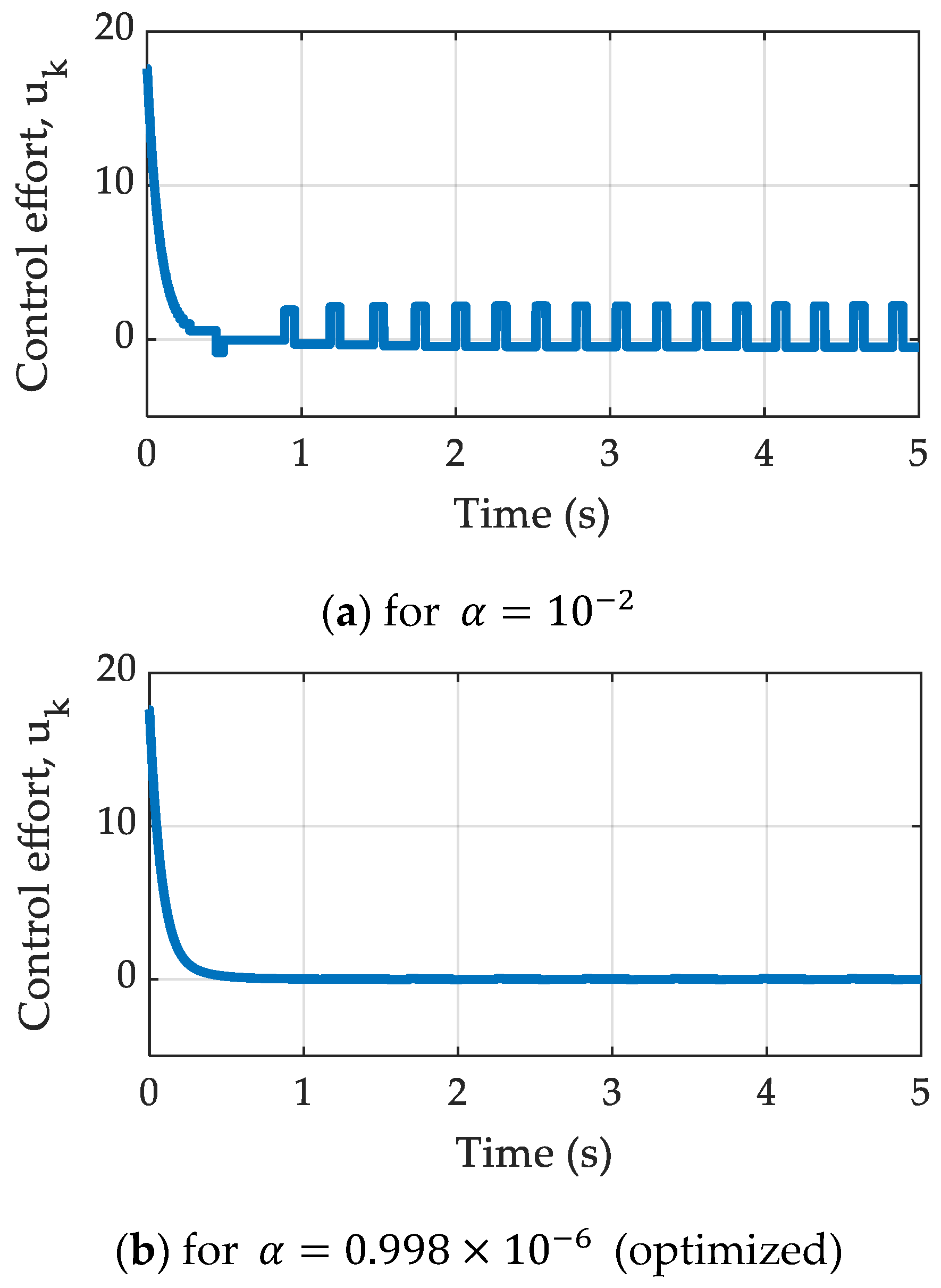
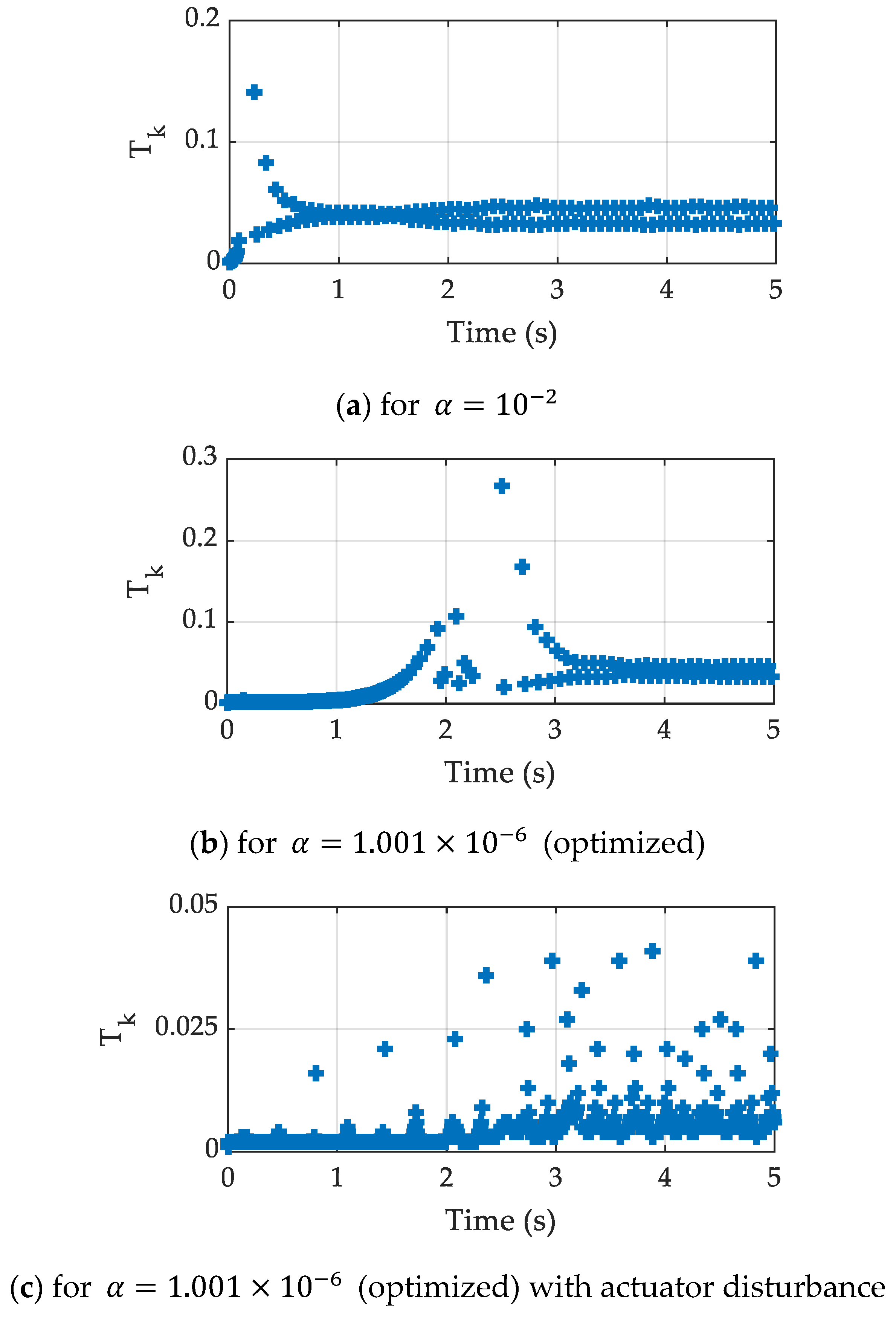
4. Simulation Results

In this section, we have performed simulations using MATALB software for implementing the ETC scheme on an inverted pendulum and single-link robot system. In ETC, suppose that the kth triggering instant is t_k and the next triggering instant is defined by t_k+1, then the inter event execution time, T_k, is represented as:

$$T_k=t_{k+1}-t_k$$

(72)

where $T_k\ge T_{min}$. The T_min is the lower bound on T_k and $T_{min}=1ms$. The $T_{min}=1ms$ is also the sampling time set for running the simulations in MATLAB software. If $T_k<T_{min}$, then many sampling instants will not be captured by the MATLAB processor. Hence, the minimum inter-event execution time, $T_k$, will always be greater than or equal to $T_{min}$. If the $T_{min}$ is reduced below 1 ms, then the computation time increases significantly. However, with high-speed computers, the $T_{min}$ can be reduced to values below 1 ms as well. The upper bound on T_k is governed by an event triggering mechanism which has been developed in Section 3.

4.1. Case Study 1: Stabilization of Inverted Pendulum System

The simulation results for the stabilization of the inverted pendulum system have been obtained using parameters given in

Table 1. Inverted Pendulum System and Controller Parameters.

M (Kg)	m (Kg)	l (m)	g (m/s2)	k1	k2	η
1	0.1	0.3	9.8	5	5	1

.

Table 2. Fitness Function and Number of Samples for Inverted Pendulum System.

Value of α	Fitness Function Jfit (t)	Number of Samples
10−1	72.13	147
10−2	22.92	211
10−3	8.15	276
10−4	2.70	335
10−5	1.21	394
10−6	0.85	508
10−7	0.86	630
10−8	0.91	736
10−9	1.01	866
10−10	1.12	969
0.998 × 10−6	0.8369	501

presents an analysis of the inverted pendulum system for different values of triggering parameter $\alpha$. It is observed that for lower values of the $\alpha$, the value of fitness function $J_{fit}\left(t\right)$ is very high, whereas the lowest number of samples is needed to be sent to the controller. On the increase in $\alpha$ value, the $J_{fit}\left(t\right)$ starts decreasing, whereas the number of samples goes on increasing. However, after a certain value of $\alpha$, both the $J_{fit}\left(t\right)$ and number of samples start increasing. Hence, it is required to find the optimum value of $\alpha$ so that both the fitness function $J_{fit}\left(t\right)$ and number of samples are at the minimum level.

The $J_{fit}\left(t\right)$ is further minimized using the PSO algorithm and an optimized value of $\alpha$ is obtained. The simulation parameters taken for running the PSO algorithm are as follows: (i) number of iterations = 50, (ii) number of particles = 20 and (iii) total simulation period $T_s=20s$. The other PSO parameters have been taken from Mishra and Chandra et al. (2014). Now, the optimized value of $\alpha$ is given in the bottom row of Table 2. The value of fitness function $J_{fit}\left(t\right)$ is 0.8369, which is the minimum among all fitness values given in Table 2. The number of samples needed is 501, which is very low if we compare it with a periodic sampling of 1 ms. If $T_s=20s$ then it would require 20,001 samples in case of periodic sampling.

Next, the inverted pendulum system performance has been evaluated by analyzing the behavior of its system states, control effort and inter-event execution time waveforms, which are shown Figure 3, Figure 4 and Figure 5. Two situations of norm of system states, $\Vert X\left(t\right)\Vert$, for $\alpha ={10}^{-2}$ (very high) and $\alpha =0.998\times {10}^{-6}$ (optimized), are shown in Figure 3. For a relatively higher value of $\alpha$ as shown in Figure 3a, the system states have very poor performance, while the number of samples is 211. For the optimized case as shown in Figure 3b, the system states performance is very satisfactory, whereas the number of samples needed is just 501.

Similarly, in Figure 4, the control effort waveforms are shown for $\alpha ={10}^{-2}$ (very high) and $\alpha =0.998\times {10}^{-6}$ (optimized). Again, the performance of the optimized case is superior to the case of Figure 4a. Hence, it can be said that minimum control effort could be maintained with a very low number of samples as well. The inter-event execution time, $T_k$, waveforms are shown in Figure 5. It is already explained that the lowest number of triggering samples is required in the optimized case.

4.2. Case Study 2: Stabilization of Single-Link Robot System

We will now discuss the simulation results of the single-link robot system. The simulation results for the stabilization of the single-link robot system have been obtained using parameters given in

Table 3. Single-Link Robot and Controller Parameters.

J	m (Kg)	l (m)	g (m/s2)	k1	k2	η
0.5	0.1	0.3	9.8	2	10	1

.

Table 4. Fitness Function and Number of Samples for Single-Link Robot.

Value of α	Fitness Function Jfit (t)	Number of Samples
10−1	78.33	509
10−2	25.47	521
10−3	8.56	538
10−4	3.287	556
10−5	1.71	693
10−6	1.49	971
10−7	1.60	1240
10−8	1.82	1511
10−9	2.09	1782
10−10	2.35	2057
1.001 × 10−6	1.488	968

presents an analysis of the single-link robot system for different values of triggering parameter $\alpha$. It is observed that for lower values of the $\alpha$, the value of fitness function $J_{fit}\left(t\right)$ is very high, whereas the lowest number of samples needed to be sent to the controller. On the increase in $\alpha$ value, the $J_{fit}\left(t\right)$ starts decreasing, whereas the number of samples goes on increasing. However, after a certain value of $\alpha$, both the $J_{fit}\left(t\right)$ and number of samples start increasing. Hence, it is required to find the optimum value of $\alpha$ so that both the fitness function $J_{fit}\left(t\right)$ and number of samples are at the minimum level.

The $J_{fit}\left(t\right)$ is further minimized using the PSO algorithm, and an optimized value of $\alpha$ is obtained. The optimized value of $\alpha$ is given in the bottom row of Table 4. The value of fitness function $J_{fit}\left(t\right)$ is 1.488, which is the minimum among all fitness values given in Table 4. The number of samples needed is 968, which is very low if we compare it with a periodic sampling of 1 ms. If $T_s=20s$ then it would require 20,001 samples in case of periodic sampling.

The simulation results for single-link robot system states, control effort and inter-event execution time waveforms are shown in Figure 6, Figure 7 and Figure 8. Three situations of norm of system states, $\Vert X\left(t\right)\Vert$, for $\alpha ={10}^{-2}$ (very high), $\alpha =1.001\times {10}^{-6}$ (optimized) and $\alpha =1.001\times {10}^{-6}$ (optimized) with actuator disturbance, are shown in Figure 6. For a relatively higher value of $\alpha$ as in Figure 6a, the system states have very poor performance, while the number of samples is 521. For the optimized case in Figure 6b, the system states performance is better compared to the case of Figure 6a, and the number of samples needed is just 968. Next, in Figure 6c, the performance of the system states is slightly affected by the actuator disturbance. However, the states always remain in the stability region provided that the disturbance signal is bounded within a small range.

In Figure 7, the control effort waveforms are shown for $\alpha ={10}^{-2}$ (very high), $\alpha =1.001\times {10}^{-6}$ (optimized) and $\alpha =1.001\times {10}^{-6}$ (optimized) with actuator disturbance. Again, the performance of the optimized case (Figure 7b) is much better than that of Figure 7a. Hence, it can be said that minimum control effort could be maintained with an optimized triggering parameter. As shown in Figure 7c, a slightly high control effort is required to keep the system states in stable trajectory due to disturbance added in the actuator signal. However, it is important to notice that the proposed ETC scheme works absolutely fine for small disturbances. Figure 8 presents the inter-event execution time, T_k. The range of T_k is between 0.001 and 0.15 s for $\alpha ={10}^{-2}$ (very high), as shown in Figure 8a, whereas for $\alpha =1.001\times {10}^{-6}$ (optimized) it is between 0.001 and 0.28 s, as shown in Figure 8b. For the third case with actuator disturbance as shown in Figure 8c, the range of T_k lies between 0.001 and 0.045 s. This is due to the fact that the number of control updates would increase when a continuous disturbance signal affects the actuator/control signal.

The chattering can also be observed in non-optimized event-triggered control cases (e.g., Figure 3a, Figure 4a, Figure 6a, and Figure 7a). The optimized event-triggered control cases do not show any chattering (e.g., Figure 3b, Figure 4b, Figure 6b, and Figure 7b).

Finally, we consider the non-zero value of x_1d, i.e., trajectory tracking control of the proposed scheme. The reference trajectory for this objective is considered as $x_{1d}=0.1\sin \left(0.2\pi t\right)$. Next, the reference trajectory for the second system state is evaluated using the expression of Equation (8) for i = 1. Hence, the x_2d is given as:

$$x_{2d}=g_1^{-1}\left[{\dot{x}}_{1d}-f_1+k_1·{\tilde{x}}_1\right]$$

(73)

Based on the above reference trajectories, $x_{1d}$ and $x_{2d}$, the closed-loop system has been simulated and the results are shown in Figure 9. It should be noted that the closed-loop response shown in Figure 9 is obtained only for the optimized event-triggered control for $\alpha =1.001\times {10}^{-6}$. All other cases have been described in Figure 7, Figure 8 and Figure 9. As shown in the figure, the proposed controller forces the system states (in Figure 9a,b) to follow the desired trajectory very satisfactorily. Similarly, the control effort does not vary after 1 s duration (in Figure 9c). However, the inter-event time (in Figure 9d) has been reduced as compared to the previous cases. It is due to variable reference trajectories where a continuous control command update is required. In cases where the control command does not need regular updates, the number of data samples is minimized significantly. This has been demonstrated in the case of x_1d = 0.

5. Conclusions

This paper presented an ETC scheme for an NCS. Initially, a backstepping control law was designed for a nonlinear system in strict-feedback form. Thereafter, an optimized event triggering algorithm by assuring the closed-loop stability of the system was developed. Later, the proposed ETC scheme was implemented on two case studies of an inverted pendulum and single-link robot system. Next, the simulations were performed to verify the effectiveness of the proposed ETC scheme. The performance of the system states, control efforts, state error due to non-uniform sampling and event execution time interval was analyzed for both the nonlinear systems. The proposed ETC scheme can be applied to any generalized nonlinear system provided it is in the strict-feedback form. Another important contribution of this study is the optimized event triggering algorithm that helps the ETC to maintain the optimum performance of the nonlinear system with a reduced number of samples required to be sent over the communication channel. As compared to the non-optimized event triggering algorithm, the optimized event triggering algorithm takes more triggering pulses but provides very efficient tracking of state trajectories. The non-optimized event triggering parameter reduces the triggering samples but leads to the degradation of system performance, as shown in simulation results. The effects of a communication network for data transmission have not been taken into account in the present work, which might be the focus of future work.

References

1. Åarzén, K.-E. A Simple Event-Based PID Controller. IFAC Proc. Vol. 1999, 32, 8687–8692. [Google Scholar] [CrossRef]
2. Heemels, W.P.M.H.; Sandee, J.H.; Van Den Bosch, P.P.J. Analysis of Event-Driven Controllers for Linear Systems. Int. J. Control 2008, 81, 571–590. [Google Scholar] [CrossRef]
3. Vamvoudakis, K.G. Event-Triggered Optimal Adaptive Control Algorithm for Continuous-Time Nonlinear Systems. IEEE/CAA J. Autom. Sin. 2014, 1, 282–293. [Google Scholar] [CrossRef]
4. Sahoo, A.; Xu, H.; Jagannathan, S. Neural Network-Based Event-Triggered State Feedback Control of Nonlinear Continuous-Time Systems. IEEE Trans. Neural Netw. Learn. Syst. 2016, 27, 497–509. [Google Scholar] [CrossRef]
5. Yu, H.; Hao, F. Input-to-State Stability of Integral-Based Event-Triggered Control for Linear Plants. Automatica 2017, 85, 248–255. [Google Scholar] [CrossRef]
6. Wang, A.; Liu, L.; Qiu, J.; Feng, G. Event-Triggered Robust Adaptive Fuzzy Control for a Class of Nonlinear Systems. IEEE Trans. Fuzzy Syst. 2019, 27, 1648–1658. [Google Scholar] [CrossRef]
7. Lu, W.; Yin, X.; Fu, Y.; Gao, Z. Observer-Based Event-Triggered Predictive Control for Networked Control Systems under Dos Attacks. Sensors 2020, 20, 6866. [Google Scholar] [CrossRef] [PubMed]
8. Mazo, M.; Tabuada, P. Special Issue Technical Notes and Correspondence: Decentralized Event-Triggered Control over Wireless Sensor/Actuator Networks. IEEE Trans. Automat. Control 2011, 56, 2456–2461. [Google Scholar] [CrossRef] [Green Version]
9. Tripathy, N.S.; Kar, I.N.; Paul, K. An Event-Triggered Based Robust Control of Robot Manipulator. In Proceedings of the 2014 13th International Conference on Control Automation Robotics and Vision, ICARCV, Singapore, 10–12 December 2014; pp. 425–430. [Google Scholar] [CrossRef]
10. Bhadu, M.; Tripathy, N.S.; Kar, I.N.; Senroy, N. Event-Triggered Communication in Wide-Area Damping Control: A Limited Output Feedbackbased Approach. IET Gener. Transm. Distrib. 2016, 10, 4094–4104. [Google Scholar] [CrossRef] [Green Version]
11. Mahmoud, M.S.; Sabih, M. Networked Event-Triggered Control: An Introduction and Research Trends. Int. J. Gen. Syst. 2014, 43, 810–827. [Google Scholar] [CrossRef]
12. Gautam, M.K.; Pati, A.; Mishra, S.K.; Appasani, B.; Kabalci, E.; Bizon, N.; Thounthong, P. A Comprehensive Review of the Evolution of Networked Control System Technology and Its Future Potentials. Sustainability 2021, 13, 2962. [Google Scholar] [CrossRef]
13. Behera, A.K.; Bandyopadhyay, B. Self-Triggering-Based Sliding-Mode Control for Linear Systems. IET Control Theory Appl. 2015, 9, 2541–2547. [Google Scholar] [CrossRef]
14. Behera, A.K.; Bandyopadhyay, B. Event-Triggered Sliding Mode Control for a Class of Nonlinear Systems. Int. J. Control 2016, 89, 1916–1931. [Google Scholar] [CrossRef]
15. Behera, A.K.; Bandyopadhyay, B. Robust Sliding Mode Control: An Event-Triggering Approach. IEEE Trans. Circuits Syst. II Express Briefs 2017, 64, 146–150. [Google Scholar] [CrossRef]
16. Postoyan, R.; Tabuada, P.; Nesic, D.; Anta, A. Event-Triggered and Self-Triggered Stabilization of Distributed Networked Control Systems. In Proceedings of the 2011 50th IEEE Conference on Decision and Control and European Control Conference, Orlando, FL, USA, 12–15 December 2011; pp. 2565–2570. [Google Scholar] [CrossRef] [Green Version]
17. Abdelrahim, M.; Postoyan, R.; Daafouz, J.; Nešić, D. Stabilization of Nonlinear Systems Using Event-Triggered Output Feedback Controllers. IEEE Trans. Automat. Control 2016, 61, 2682–2687. [Google Scholar] [CrossRef] [Green Version]
18. Jiao, J.; Wang, G. Event Driven Tracking Control Algorithm for Marine Vessel Based on Backstepping Method. Neurocomputing 2016, 207, 669–675. [Google Scholar] [CrossRef]
19. Li, Y.X.; Yang, G.H. Model-Based Adaptive Event-Triggered Control of Strict-Feedback Nonlinear Systems. IEEE Trans. Neural Networks Learn. Syst. 2018, 29, 1033–1045. [Google Scholar] [CrossRef] [PubMed]
20. Li, Y.X.; Yang, G.H. Event-Triggered Adaptive Backstepping Control for Parametric Strict-Feedback Nonlinear Systems. Int. J. Robust Nonlinear Control 2018, 28, 976–1000. [Google Scholar] [CrossRef]
21. Mishra, S.K.; Purwar, S.; Kishor, N. Event-Triggered Nonlinear Control of OWC Ocean Wave Energy Plant. IEEE Trans. Sustain. Energy 2018, 9, 1750–1760. [Google Scholar] [CrossRef]
22. Mishra, S.K.; Appasani, B.; Jha, A.V.; Garrido, I.; Garrido, A.J.; Costa Castelló, R. Centralized Airflow Control to Reduce Output Power Variation in a Complex OWC Ocean Energy Network. Complexity 2020. [Google Scholar] [CrossRef]
23. Zhang, C.H.; Yang, G.H. Event-Triggered Control for a Class of Strict-Feedback Nonlinear Systems. Int. J. Robust Nonlinear Control 2019, 29, 2112–2124. [Google Scholar] [CrossRef]
24. Huang, J.; Wang, Q.G. Event-Triggered Adaptive Control of a Class of Nonlinear Systems. ISA Trans. 2019, 94, 10–16. [Google Scholar] [CrossRef] [PubMed]
25. Xing, L.; Wen, C.; Liu, Z.; Su, H.; Cai, J. Event-Triggered Output Feedback Control for a Class of Uncertain Nonlinear Systems. IEEE Trans. Automat. Control 2019, 64, 290–297. [Google Scholar] [CrossRef]
26. Li, T.; Wen, C.; Yang, J.; Li, S.; Guo, L. Event-Triggered Tracking Control for Nonlinear Systems Subject to Time-Varying External Disturbances. Automatica 2020, 119. [Google Scholar] [CrossRef]
27. Xu, B.; Liu, X.; Wang, H.; Zhou, Y. Event-Triggered Control for Nonlinear Systems via Feedback Linearisation. Int. J. Control 2020, 1–11. [Google Scholar] [CrossRef]
28. Hu, X.; Yu, H.; Hao, F. Lyapunov-Based Event-Triggered Control for Nonlinear Plants Subject to Disturbances and Transmission Delays. Sci. China Inf. Sci. 2020, 63. [Google Scholar] [CrossRef] [Green Version]
29. Zou, K.; Cai, Y.; Chen, L.; Sun, X. Event-Triggered Nonlinear Model Predictive Control for Trajectory Tracking of Unmanned Vehicles. Proc. Inst. Mech. Eng. Part D J. Automob. Eng. 2021. [Google Scholar] [CrossRef]
30. Cui, L.; Zhang, Y.; Wang, X.; Xie, X. Event-Triggered Distributed Self-Learning Robust Tracking Control for Uncertain Nonlinear Interconnected Systems. Appl. Math. Comput. 2021, 395. [Google Scholar] [CrossRef]
31. Su, X.; Wen, Y.; Shi, P.; Wang, S.; Assawinchaichote, W. Event-Triggered Fuzzy Control for Nonlinear Systems via Sliding Mode Approach. IEEE Trans. Fuzzy Syst. 2021, 29, 336–344. [Google Scholar] [CrossRef]
32. Mishra, S.K.; Pati, A.; Appasani, B.; Jha, A.V.; Kumar, M.R.; Pal, V.C.; Gautam, M.K. Event-Triggered Fractional-Order PID Control of Fractional-Order Networked Control System. In Lecture Notes in Electrical Engineering; Springer: Berlin/Heidelberg, Germany, 2021; Volume 690, pp. 205–216. [Google Scholar] [CrossRef]
33. Clerc, M. Particle Swarm Optimization; ISTE Ltd.: London, UK, 2010. [Google Scholar] [CrossRef]
34. Wang, J.J. Simulation Studies of Inverted Pendulum Based on PID Controllers. Simul. Model. Pract. Theory 2011, 19, 440–449. [Google Scholar] [CrossRef]
Figure 1. Block diagram of ETC for NCS.
Mathematics 09 01262 g001
Figure 2. Block diagram for optimizing triggering parameter α based on PSO (offline tuning).
Mathematics 09 01262 g002
Figure 3. Inverted pendulum system states, X .
Mathematics 09 01262 g003
Figure 4. Control effort, uk.
Mathematics 09 01262 g004
Figure 5. Inter event execution time, Tk.
Mathematics 09 01262 g005
Figure 6. Single-link robot system states, X .
Mathematics 09 01262 g006
Figure 7. Control effort, uk.
Mathematics 09 01262 g007
Figure 8. Inter event execution time, Tk.
Mathematics 09 01262 g008
Figure 9. Closed-loop response for trajectory tracking control using optimized event-triggered control.
Mathematics 09 01262 g009