Optimal Parameter Estimation Methodology of Solid Oxide Fuel Cell Using Modern Optimization

Abstract

An optimal parameter estimation methodology of solid oxide fuel cell (SOFC) using modern optimization is proposed in this paper. An equilibrium optimizer (EO) has been used to identify the unidentified parameters of the SOFC equivalent circuit with the assistance of experimental results. This is presented via formulating the modeling process as an optimization problem considering the sum mean squared error (SMSE) between the observed and computed voltages as the target. Two modes of the SOFC-based model are investigated under variable operating conditions, namely, the steady-state and the dynamic-state based models. The proposed EO results are compared to those obtained via the Archimedes optimization algorithm (AOA), Heap-based optimizer (HBO), Seagull Optimization Algorithm (SOA), Student Psychology Based Optimization Algorithm (SPBO), Marine predator algorithm (MPA), Manta ray foraging optimization (MRFO), and comprehensive learning dynamic multi-swarm marine predators algorithm. The minimum fitness function at the steady-state model is obtained via the proposed EO with value of 1.5527 × 10⁻⁶ at 1173 K. In the dynamic based model, the minimum SMSE is 1.0406. The obtained results confirmed the reliability and superiority of the proposed EO in constructing a reliable model of SOFC.

1. Introduction

There is a growing demand for energy to meet the requirements of continuous industrial development and modern civilization. In parallel, there is a growing concern about the depletion of traditional energy sources such as fossil fuel and drawbacks of continuous consumption of fossil fuel such as climate change [1]. Indeed, a recent study expected that future energy demands might exceed the limits of current energy systems [2]. Moreover, the increasing global energy demands and consumption of fossil fuel will escalate the emissions of greenhouse gases and other toxic air pollutants. Therefore, alternative sources of energy such as renewable energy have earned significant attention in the recent decades. In particular, fuel cell is among the power generation systems that can deliver environmentally friendly quality energy with great energy conversion efficiency. Furthermore, fuel cell has a great potential in power delivery for stationary and movable applications compared to other storage technologies [3,4,5,6,7]. Other remarkable features of fuel cell over other energy alternatives include lower fuel oxidation temperature and reduced emissions [8]. Solid oxide fuel cell (SOFC) and polymer composites-based electrolyte fuel cell represent the most attractive types of fuel cell for a wide range of applications. A growing effort is made to deliver a model that can predict the performance of fuel cell over steady state or dynamics operating environmental conditions [9,10,11,12]. In fact, appropriate model identification requires feeding accurate input parameters to the governing equations that encompass physical and chemical properties of the cell, where the modelling methodologies can be empirical, semi-empirical, or theoretical [13,14,15,16].

The parameter extraction of the fuel cell model plays an important role in the simulation, evaluation, control, and optimization of a fuel cell system. The voltage drops in SOFC are mainly reliant on the parameters associated with the chemical processes inside SOFC [17,18]. Several methods were used to identify the accurate parameters of SOFC. Among these methods, the metaheuristic optimization-based methodologies were superior in resolving the SOFC parameter estimation problem due to their reliability, robustness, and simplicity. Shi et al. [19] proposed a strategy, Converged Grass Fibrous Root, to determine the best parameters of the SOFC model. Both temperature and pressure variation are considered. During the optimization process, seven parameters are assigned to be decision variables: the standard potential, the current limitation density, the Tafel line slope, a constant depends on the operating state of SOFC, the area-specific resistance, the anode exchange current density, and the cathode exchange current density. El-Hay et al. [10] suggested a methodology based on an interior search algorithm to estimate the steady state and transient parameters of SOFC. A proportional-integral controller is integrated with the dynamic model to enhance its performance throughout transient disturbances. A similar study also carried by the same authors based on Satin Bowerbird Optimizer was conducted [9]. During the optimization process, the decision variables are represented by the unknown parameters of SOFC, whereas the cost function is represented by mean squared deviations between experimental data and estimated SOFC voltages. In the same direction, Yousri et al. [20] proposed a modified algorithm called comprehensive learning dynamic multi-swarm marine predators to determine both static and dynamic parameters of SOFC. During the optimization process, the mean squared error between the experimental data and estimated SOFC voltage is used as the objective function that is required to be minimum. Nassef et al. [21] used the radial movement optimization algorithm (RMOA) to determine the best parameters of the SOFC model. The model of SOFC was created using a neural network. During the optimization process, four parameters, including electrolyte thickness, cathode interlayer thickness, anode porosity, and anode support layer thickness, are used as decision variables; in contrast, the objective function is represented by the power density of SOFC. By using the RMOA, the power density was increased by 17.28% compared with the genetic algorithm. In the same direction, Fathy et al. [22] suggested a methodology based on the moth-flame optimization algorithm (MFOA). The power density of SOFC using the MFOA was improved. It was increased by 18.92% and 5.56% compared to the genetic algorithm and RMOA, respectively.

The contribution of the current research work can be summarized as follows:

• A novel approach based on Equilibrium Optimizer (EO) is suggested to determine the optimal parameters of the SOFC-based model.
• The suggested methodology is validated through both steady-state and dynamic-state models of SOFC with the changing of the operational conditions.
• A comprehensive comparison with previous works and other programs of the Archimedes optimization algorithm (AOA), Heap-based optimizer (HBO), Seagull Optimization Algorithm (SOA), Student Psychology Based Optimization Algorithm (SPBO), Marine predator algorithm (MPA), and Manta ray foraging optimization (MRFO).
• The superiority and reliability of the suggested EO-based strategy in solving the SOFC parameter determination problem is verified.

The rest of the paper is organized as follows: The mathematical model of SOFC is illustrated in Section 2. Section 3 presents an overview about main aspects of the equilibrium optimizer. Then, the suggested optimization problem and solution methodology are explained in Section 4. Section 5 presents a detailed discussion of the obtained results and a comparative study with other methods. Finally, the main findings and the future work are outlined in Section 6.

2. SOFC Mathematical Model

In this section, the authors illustrate the static- and dynamic-based models of SOFC.

2.1. Steady-State Model

The output voltage of SOFC can be estimated using the following relation considering the activation loss, ohmic loss, and concentration loss [23]:

$$V_{cell}=E_n-V_a-V_o-V_c$$

(1)

where E_n denotes the reversible voltage of the cell, and V_a, V_o, and V_c denote the activation, ohm, and concentration voltage drops, respectively.

The activation loss, concentration loss and ohmic loss can be estimated using the following relations:

$$V_a=a\cdot \ln \left(\frac{J}{2J_0}\right)$$

(2)

$$V_o={\displaystyle \sum _{k}i\times R_k}$$

(3)

$$V_c=-b\cdot \ln \left(1-\frac{J}{J_{\max }}\right)$$

(4)

where a and b are constants; J denotes the current density; J₀ denotes the exchange current density; J_max is the maximum current density; R_k is the sum of ionic (electrolyte) and electronic resistances; and i denotes the output SOFC current.

To increase the rating voltage of SOFC, the number of cells are connected in series. Therefore, the total stack output voltage can be estimated using the following relation.

$$V_s=n_c\times V_{cell}=n_c\times \left(E_n-V_a-V_o-V_c\right)$$

(5)

where vs. is the stack voltage and n_c is the number of cells. The reversible voltage can be written as follows [24]:

$$E_n=E_0+\frac{RT}{2F}\ln \left(\frac{P_{H_2}\sqrt{P_{O_2}}}{P_{H_{2}O}}\right)$$

(6)

where E₀ denotes the reference voltage at unit activity and atmospheric pressure; T denotes operating temperature (K); P_H2, P_O2, and P_H2O denote the hydrogen, oxygen, and water partial pressures, respectively; R is the universal gas constant with a value of 8.314 kJ (kmol K)⁻¹; and F is the Faraday constant.

2.2. SOFC Dynamic Model

The gas molar flow in SOFC is reliant on hydrogen and oxygen partial pressures as follows [24]:

$$\frac{q_{H_2}}{P_{H_2}}=\frac{k_{an}}{\sqrt{M_{H_2}}}=K_{H_2}$$

(7)

$$\frac{q_{O_2}}{P_{O_2}}=\frac{k_{an}}{\sqrt{M_{O_2}}}=K_{O_2}$$

(8)

where q_H2 is the molar flow of hydrogen; q_O2 is the molar flow of oxygen; K_H2 is the hydrogen molar constant; K_O2 is the oxygen molar constant; k_an is the anode valve constant; M_H2 is the molar masses of hydrogen; and M_O2 is the molar masses of oxygen.

The partial pressure derivative can be estimated using the following relation:

$$\frac{d{P}_{H_2}}{dt}=\frac{RT}{V_{an}}\left(q_{H_2}{}^{in}-q_{H_2}{}^{out}-q_{H_2}{}^r\right)$$

(9)

where V_an denotes the anode volume; q_H2ⁱⁿ is the hydrogen input flow rate; q_H2^out is the hydrogen output flow rate; and q_H2^r denotes the reacted hydrogen flow rate.

The reacted hydrogen flow rate can be estimated based on the following relation:

$$q_{H_2}{}^r=\frac{n_{c}i}{2F}=2K_{r}i$$

(10)

where K_r is constant.

Considering the above equations and the Laplace transform, hydrogen and oxygen partial pressures can be formulated as follows.

$$P_{H_2}(s)=\frac{\raisebox{1ex}{$1$}\!\left/ \!\raisebox{-1ex}{$K_{H_2}$}\right.}{1+{\tau }_{H_2}}\left(q_{H_2}{}^{in}-2K_{r}i\right)$$

(11)

$$P_{H_{2}O}(s)=\frac{\raisebox{1ex}{$1$}\!\left/ \!\raisebox{-1ex}{$K_{H_{2}O}$}\right.}{1+{\tau }_{H_{2}O}}\left(2K_{r}i\right)$$

(12)

$$P_{O_2}(s)=\frac{\raisebox{1ex}{$1$}\!\left/ \!\raisebox{-1ex}{$K_{O_2}$}\right.}{1+{\tau }_{O_2}}\left(q_{O_2}{}^{in}-K_{r}i\right)$$

(13)

where τ_H2, τ_H2O, and τ_O2 denote the flow time constants of hydrogen, water, and oxygen, respectively.

Ultimately, the dynamic model of SOFC voltage is given by the following relation.

$$V_s=n_c\left(E_0+\frac{RT}{2F}\left(\ln \frac{P_{H_2}\sqrt{P_{O_2}}}{P_{H_2}}\right)\right)-\left(a\cdot \ln \left(\frac{J}{2J_0}\right)+r\times i-b\cdot \ln \left(1-\frac{J}{J_{\max }}\right)\right)$$

(14)

3. Overview of Equilibrium Optimizer

Equilibrium optimizer (EO) is a recent algorithm that was proposed by Faramarzi et al. in 2020 [25]. The core idea of the EO is extracted from the control volume mass balance models. During the optimization process of the EO, the particles and positions are assigned to the solutions and concentrations, respectively. The details explanations about the inspiration, mathematical model, and algorithm of the EO can be found in [25]. The mass balance formula is expressed as follows.

$$V\frac{dC}{dt}=Q{C}_{eq}-QC-G$$

(15)

where C denotes the concentration of the control volume; $V\frac{dC}{dt}$ denotes the changing rate of the mass; Q denotes the flow rate; C_eq denotes the concentration at the balance state; and G denotes the mass generation rate.

By integration over time and rearranged with the above formula, the following relation can be used to express the concentration of the control volume.

$$C=C_{eq}+(C_0-C_{eq})F+\frac{G}{\lambda V}(1-f)$$

(16)

where λ denotes the turnover rate ($\lambda =\raisebox{1ex}{$Q$}\!\left/ \!\raisebox{-1ex}{$V$}\right.$) and $f=e^{-\lambda (t-t_0)}$, and t₀ and C₀ denote the initial time and concentration, respectively.

The time t is decreasing with increasing the number of iterations as follows:

$$t={(1-\raisebox{1ex}{$I$}\!\left/ \!\raisebox{-1ex}{$z$}\right.)}^{\left(a_2\frac{I}{z}\right)}$$

(17)

$$\overrightarrow{t_0}=\frac{1}{\overrightarrow{\lambda }}\ln (-a_{1}sign(\overrightarrow{r}-0.5)[1-e^{\overrightarrow{\lambda t}}])+t$$

(18)

$$\overrightarrow{F}=a_{1}sign(\overrightarrow{r}-0.5)[1-e^{\overrightarrow{\lambda t}}]$$

(19)

where I and z are the current iteration and maximum number of iterations, respectively. a₁ and a₂ are constants. $\overrightarrow{r}$ is a random vector in range [0, 1].

Considering Equation (16), there are three sections describing the updating process for particles. The first section represents the equilibrium concentration. It represents the optimum solutions arbitrarily chosen from a pool. The second section is related to the concentration variations between a particle and the equilibrium state. The last section is related to the generation rate. It is mainly performing the role of an exploiter. The equilibrium state is the final convergence state of the EO optimization process. The equilibrium pool can be represented as follows.

$${\overrightarrow{C}}_{eq.pool}=\left\{{\overrightarrow{C}}_{eq(1)},{\overrightarrow{C}}_{eq(2)},{\overrightarrow{C}}_{eq(3)},{\overrightarrow{C}}_{eq(4)},{\overrightarrow{C}}_{eq(ave)}\right\}$$

(20)

During the first iteration, the particle modifies the concentration using ${\overrightarrow{C}}_{eq(1)}$ whereas it is uses ${\overrightarrow{C}}_{eq(ave)}$ with other iterations. The generation rate is defined as follows.

$$\overrightarrow{G}=\overrightarrow{G_0}{e}^{-\overrightarrow{k}(t-t_0)}$$

(21)

where G₀ is the initial value, and k denotes a decay constant (k = λ).

$$\overrightarrow{G}=\overrightarrow{G_0}{e}^{-\overrightarrow{\lambda }(t-t_0)}=\overrightarrow{G_0}\overrightarrow{F}$$

(22)

$$\overrightarrow{G_0}=\overrightarrow{GCP}{\overrightarrow{(C}}_{eq}-\overrightarrow{\lambda }\overrightarrow{C})$$

(23)

$$\overrightarrow{GCP}=\left\{\begin{array}{ll}0.5r_1& r_2\ge GP\\ 0& r_2<GP\end{array}\right.$$

(24)

where r₁ and r₂ are random variables in range [0, 1], and GCP is a parameter that controls the generation rate.

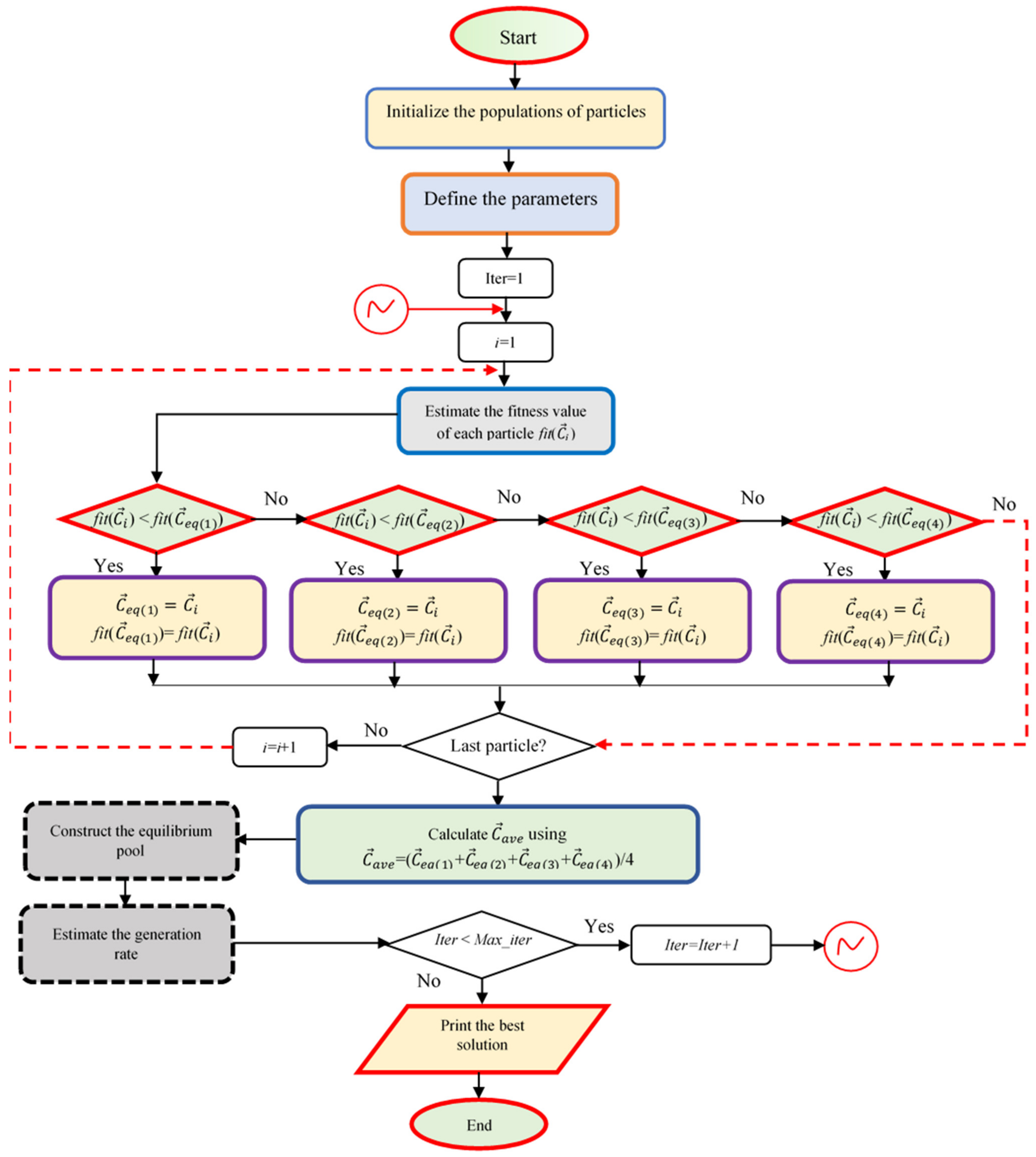
The addition of memory saving helps each particle to save its coordinates in the search space. Moreover, it informs its fitness function value. The fitness function related to a particular particle in the ongoing iteration is compared with the previous one; then, the updating process is placed if it reaches better fit. This action enhances the exploitation phase. The optimization process of EO is illustrated in Figure 1.

4. The Proposed Methodology

In this section, the proposed methodology is explained via formulating the problem of SOFC parameter estimation as an optimization problem, and an objective function and corresponding constraints are also introduced. Moreover, the proposed solution methodology is also presented.

4.1. The Proposed Objective Function

In this section, the formulation of the identification process of SOFC circuit’s parameters as an optimization problem is explained via specifying the fitness function, the corresponding constraints, and the proposed methodology of the solution incorporated by the EO. The main target of the work is to construct a reliable equivalent circuit of SOFC by identifying six parameters, E₀, a, J_o, r, b, and J_max; this is achieved with the aid of experimental data of the current and voltage of FC. The fitness function represented in this work is the sum mean squared error between the measured and calculated terminal voltages of SOFC, and this can be described as follows:

$$\begin{array}{cc}Minimize& \end{array}SMSE={\displaystyle \sum _{k=1}^N\frac{1}{N}}{\left(V_{meas,k}-V_{cal,k}\right)}^2$$

(25)

where V_meas,k and V_cal,k are the k^th observed and computed voltages, respectively, and N is the number of measured datasets. The constraints related to the variables to be designed can be described as follows:

$$\begin{array}{l}{E}_0{}^{\min }\le E_0\le E_0{}^{\max }\\ a^{\min }\le a\le a^{\max }\\ J_o{}^{\min }\le J_o\le J_o{}^{\max }\\ r^{\min }\le r\le r^{\max }\\ b^{\min }\le b\le b^{\max }\\ J_{\max }{}^{\min }\le x_6\le J_{\max }{}^{\max }\end{array}$$

(26)

where min denotes the minimum limit and max denotes the maximum limit. In this work the authors only considered the disturbance on the SOFC output voltage. However, in future work, they will consider the disturbance not only on the SOFC output but also on the SOFC input such as those given in [26,27,28,29].

4.2. The Proposed EO Based Methodology

The equilibrium optimizer is selected due to many advantages: It is simple in implementation; it achieves balance between the exploration and exploitation phases; and there is diversity between the population individuals. These features enable the algorithm to be applicable for many optimization problems. Six parameters are required to be identified such that the SMSE is minimized. The proposed methodology incorporating the EO begins by defining the specifications of SOFC and the recorded measured data of the terminal voltage. Then, an initial population with a dimension of n_pop × dim, n_pop is the population size, and dim is the problem dimension, which is constructed with the aid of the minimum and maximum limits defined by the user. The initial corresponding fitness function (SMSE) is calculated, and the iterative process is implemented by calculating the fitness function of each particle. The obtained fitness function is checked with those of the equilibrium pool to decide the updating action of each particle. After that, the condition of the last particle is investigated, and the average of the equilibrium pool is calculated, which helps in estimating the generation rate. The process is continued until the constraint of maximum iteration is achieved. At this moment, the optimal results are obtained and can be printed. The proposed methodology incorporating EO is shown in Figure 2.

5. Numerical Analysis

The analysis is performed on two modes of the SOFC operation which are steady-state and dynamic-state. Both of them are investigated under variable-operating conditions. The commercial SOFC, which is manufactured by Siemens [30], is employed in steady-state analysis. In such a case, four measured datasets are recorded at temperatures of 1073, 1173, 1213, and 1273 K, where the proposed EO size of population is assigned as 50, and the number of iterations is selected as 100. The population-based approach presented in this work has some difficulty, such as getting premature and local optima, and the authors take into consideration this problem by performing the approach with 50 independent runs, and the best one is selected as global optima. This action minimizes the problem of falling in local optima. Other metaheuristic approaches are implemented and compared to the proposed EO; these algorithms are the Archimedes optimization algorithm (AOA), Heap-based optimizer (HBO), Seagull Optimization Algorithm (SOA), Student Psychology Based Optimization Algorithm (SPBO), Marine predator algorithm (MPA), Manta ray foraging optimization (MRFO), and comprehensive learning dynamic multi-swarm marine predators algorithm CLDMMPA [20].

Table 1. The optimal parameters of SOFC steady-state based model operated at 1073 K.

	CLDMMPA [20]	MPA	HBO	SOA	MRFO	The Proposed EO
E0 (V)	0.90754	0.9127	0.91214	0.91101	0.91827	0.91056
a (V)	0.010741	0.011058	0.010929	0.020502	0.0116	0.010724
Jo (A/cm2)	0.098627	0.059994	0.063321	0.048127	0.035918	0.074522
r (kΩ∙cm2)	1.0	1.0	1.0	1.0	0.99919	1.0
b (V)	0.044104	0.042784	0.043502	0.0	0.036886	0.044165
Jmax (A/cm2)	1.0	1.0	1.0	0.64297	0.9183	1.0
Elapsed time (sec.)	NA	468.526	403.607	278.254	560.753	272.198102
SMSE	2.6906 × 10−6	2.692 × 10−6	2.7003 × 10−6	4.123 × 10−6	2.7213 × 10−6	2.6906 × 10−6

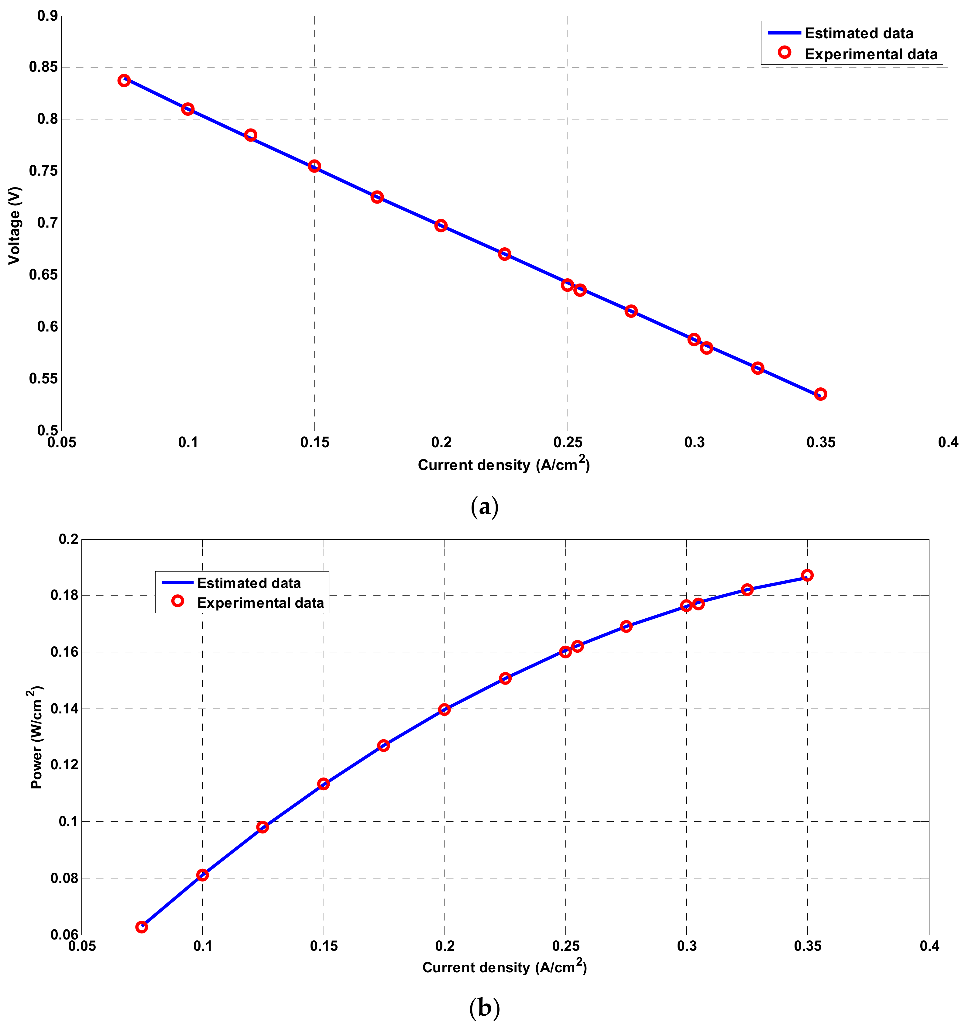
shows the obtained optimal parameters of SOFC operated at 1073 K via the proposed EO and the others. The proposed approach succeeded in achieving a fitness function of 2.6906 × 10⁻⁶ which is the same obtained via CLDMMPA. However, the CLDMMPA is complex in construction; moreover, the proposed EO consumes only 272.198102 s, which is the best compared to the others. The measured and calculated polarization curves obtained via the proposed EO are shown in Figure 3. Both curves are closely converged. Moreover, Figure 4 shows the estimated polarization curves obtained via the other approaches and the measured ones. Furthermore, the performance of each optimizer during the iterative process is shown in Figure 5. It is clear that the EO performance is the best compared to the others.

The optimal parameters of the SOFC steady-state based model at 1173, 1213, and 1273 K obtained via the proposed EO and the others are tabulated in

Table 2. The optimal parameters of SOFC steady-state based model operated at 1173 K.

	CLDMMPA [20]	MPA	HBO	SOA	MRFO	The Proposed EO
E0 (V)	0.89103	0.89129	0.89083	0.87956	0.89087	0.89108
a (V)	3.671 × 10−13	6.1748 × 10−13	3.23334 × 10−13	0.0077567	9.8137 × 10−6	3.14568 × 10−8
Jo (A/cm2)	0.095127	0.018358	0.041194	0.087363	0.068684	0.09998
r (kΩ∙cm2)	0.40473	0.41593	0.39952	0.21139	0.4027	0.40610
b (V)	0.18841	0.17741	0.19212	0.28497	0.18885	0.18741
Jmax (A/cm2)	1.0	0.98862	1.0	0.9465	0.9968	0.99999
Elapsed time (sec.)	NA	495.653992	396.181972	303.170716	612.841366	303.185040
SMSE	1.5529 × 10−6	1.5594 × 10−6	1.5557 × 10−6	3.1657 × 10−6	1.5563 × 10−6	1.5527 × 10−6

,

Table 3. The optimal parameters of SOFC steady-state based model operated at 1213 K.

	CLDMMPA [20]	MPA	HBO	SOA	MRFO	The Proposed EO
E0 (V)	0.86169	0.86189	0.86134	0.85622	0.86176	0.86164
a (V)	5.0588 × 10−13	4.2805 × 10−28	3.4456 × 10−30	3.1223 × 10−29	3.3451 × 10−5	7.12575 × 10−8
Jo (A/cm2)	0.08871	0.054568	0.011975	0.047885	0.063468	0.07768
r (kΩ∙cm2)	0.15982	0.16633	0.14858	0.000124	0.16629	0.15873
b (V)	0.28529	0.28032	0.29351	0.4012	0.27918	0.28603
Jmax (A/cm2)	1.0	0.99946	1.0	1.0	0.99732	0.99999
Elapsed time (sec.)	NA	464.968854	367.890819	236.154633	571.548052	273.530
SMSE	2.6811 × 10−6	2.6846 × 10−6	2.6887 × 10−6	4.3804 × 10−6	2.6896 × 10−6	2.6809 × 10−6

and

Table 4. The optimal parameters of SOFC steady-state based model operated at 1273 K.

	CLDMMPA [20]	MPA	HBO	SOA	MRFO	The Proposed EO
E0 (V)	0.8478	0.84782	0.84802	0.84014	0.84802	0.8478
a (V)	2.887 × 10−14	3.128 × 10−21	5.1251 × 10−6	2.238 × 10−20	3.2243 × 10−5	6.7797 × 10−12
Jo (A/cm2)	0.061816	0.014523	0.086283	0.017285	0.024437	0.0160
r (kΩ∙cm2)	0.21564	0.21634	0.22323	0.1563	0.22021	0.2169
b (V)	0.20575	0.20524	0.20009	0.36046	0.20226	0.2047
Jmax (A/cm2)	1.0	1.0	0.99984	1.00	0.99888	1.0
Elapsed time (sec.)	NA	465.757529	352.634515	199.242260	555.636660	317.980527
SMSE	2.2997 × 10−6	2.2996 × 10−6	2.3031 × 10−6	5.4888 × 10−6	2.3058 × 10−6	2.2995 × 10−6

. Regarding the obtained results at 1173 K, the best fitness function is 1.5527 × 10⁻⁶ obtained via the proposed EO while CLDMMPA comes in the second rank with a SMSE of 1.5529 × 10⁻⁶. On the other hand, the worst approach is SOA with a fitness function of 3.1657 × 10⁻⁶. Moreover, during the operation at 1213 K, the EO outperformed the others in terms of elapsed time and fitness function. The reader can see that during operation at 1273 K, the proposed EO achieved a SMSE of 2.2995 × 10⁻⁶, which is the best compared to the others.

The polarization curves of the measured data and calculated data obtained via the proposed EO for the steady-state SOFC based model at 1173, 1213, and 1273 K are shown in Figure 6. The curves confirm the matching between the experimental and calculated data.

It is important to investigate the performance of each optimizer via calculating the statistical parameters, which include the best, worst, mean, median, variance, and standard deviation after 50 independent runs. These data are calculated and tabulated in

Table 5. Statistical parameters (best, worst, mean, median, variance, and standard deviation) of all optimizers used for steady-state SOFC model.

At T = 1073 K
	Cldmmpa [20]	MPA	HBO	SOA	MRFO	The Proposed EO
Best	2.6906 × 10−6	2.69203 × 10−6	2.70035 × 10−6	4.12297 × 10−6	2.7213 × 10−6	2.6906 × 10−6
Worst	2.696 × 10−6	1.23064 × 10−5	4.49932 × 10−6	0.00034	4.8504 × 10−6	6.8151 × 10−6
Mean	2.6926 × 10−6	4.75170 × 10−6	3.11043 × 10−6	9.38355 × 10−5	3.1121 × 10−6	3.3645 × 10−6
Median	2.6917 × 10−6	3.61749 × 10−6	2.96160 × 10−6	9.33996 × 10−5	2.9395 × 10−6	2.6906 × 10−6
Variance	4.1347 × 10−18	6.38059 × 10−12	1.75759 × 10−13	9.20085 × 10−9	2.2231 × 10−13	8.38802 × 10−13
Std. deviation	2.0334 × 10−9	2.52598 × 10−6	4.19236 × 10−7	9.59210 × 10−5	4.7150 × 10−7	9.15673 × 10−7
At T = 1173 K
	CLDMMPA [20]	MPA	HBO	SOA	MRFO	The proposed EO
Best	1.5529 × 10−6	1.5594 × 10−6	1.5556 × 10−6	3.1656 × 10−6	1.5563 × 10−6	1.55279 × 10−6
Worst	1.5752 × 10−6	5.9028 × 10−6	2.1420 × 10−6	0.01102	2.6603 × 10−6	6.00407 × 10−6
Mean	1.5593 × 10−6	3.0125 × 10−6	1.6979 × 10−6	0.00026	1.7105 × 10−6	2.31364 × 10−6
Median	1.5572 × 10−6	2.4861 × 10−6	1.6532 × 10−6	1.26093 × 10−5	1.6493 × 10−6	1.58630 × 10−6
Variance	3.8987 × 10−17	1.9116 × 10−12	1.8382 × 10−14	2.42265 × 10−6	3.7587 × 10−14	2.66121 × 10−12
Std. deviation	6.244× 10−9	1.3826 × 10−6	1.3558 × 10−7	0.00155	1.9387 × 10−7	1.63132 × 10−6
At T = 1213 K
	CLDMMPA [20]	MPA	HBO	SOA	MRFO	The proposed EO
Best	2.6811 × 10−6	2.6846 × 10−6	2.6887 × 10−6	4.3804 × 10−6	2.68961 × 10−6	2.68099 × 10−6
Worst	2.7269 × 10−6	1.2325 × 10−5	3.4295 × 10−6	0.00032	3.22001 × 10−6	1.30287 × 10−5
Mean	2.6921 × 10−6	4.6204 × 10−6	2.8357 × 10−6	2.37574 × 10−5	2.85206 × 10−6	4.02438 × 10−6
Median	2.6867 × 10−6	3.3119 × 10−6	2.7703 × 10−6	1.31251 × 10−5	2.81486 × 10−6	2.78147 × 10−6
Variance	1.9891 × 10−16	9.4614 × 10−12	2.7256 × 10−14	3.77968 × 10−9	1.72574 × 10−14	1.12951 × 10−11
Std. deviation	1.4103 × 10−8	3.0759 × 10−6	1.6509 × 10−7	6.14791 × 10−5	1.3136 × 10−7	3.36081 × 10−6
At T = 1273 K
	CLDMMPA [20]	MPA	HBO	SOA	MRFO	The proposed EO
Best	2.2997 × 10−6	2.2995 × 10−6	2.30310 × 10−6	5.4888 × 10−6	2.30579 × 10−6	2.2995 × 10−6
Worst	2.3392 × 10−6	7.4728 × 10−6	3.0608 × 10−6	0.000247	2.84248 × 10−6	7.6115 × 10−6
Mean	2.3156 × 10−6	3.6859 × 10−6	2.4184 × 10−6	1.758508 × 10−5	2.40213 × 10−6	3.4890 × 10−6
Median	2.3141 × 10−6	3.1707 × 10−6	2.3647 × 10−6	7.71186 × 10−6	2.37664 × 10−6	2.3085 × 10−6
Variance	1.3448 × 10−16	2.1494 × 10−12	1.9816 × 10−14	2.25858 × 10−9	8.64055 × 10−15	4.8928 × 10−12
Std. deviation	1.1597 × 10−8	1.466 × 10−6	1.4077 × 10−7	4.7524 × 10−5	9.29545 × 10−8	2.2119 × 10−6

. The proposed EO gives acceptable statistical parameters compared to the others.

The obtained results confirmed the superiority and reliability of the proposed methodology incorporating EO in identifying the optimal parameters of the SOFC steady-state based model.

It is important to confirm the availability of the presented approach in a dynamic/transient-based model of SOFC. Therefore, a 100 kW stack with specifications given in

Table 6. SOFC stack specifications [30,31].

Parameter	Value
Prated (W)	100 kW
nc	384
E0 (V)	1.18
T (K)	1273
KH2 (kmol/s/atm)	8.43 × 10−4
KO2 (kmol/s/atm)	2.52 × 10−3
KH2O (kmol/s/atm)	2.81 × 10−4
rH-O	1.145
τH2 (s)	26.1
τO2 (s)	2.91
τH2O (s)	78.3
Te (s)	0.8

is modeled in a dynamic-state model subjected to variable load disturbances. At the beginning, the proposed EO is applied to identify the optimal parameters of a 100 kW SOFC stack operated at 1273 K; the obtained parameters are tabulated in

Table 7. The optimal parameters of SOFC dynamic-state based model operated at 1273 K.

	CLDMMPA [20]	MPA	HBO	SOA	MRFO	The Proposed EO
E0 (V)	1.1405	1.199847	1.194939	0.89461271	1.113337	1.144398
a (V)	0.037449	0.04882335	0.04756176	0.000	0.02729001	0.02982692
Jo (A/cm2)	0.095442	0.09987029	0.0939504	0.090655585	0.03143729	0.0202932
r (kΩ∙cm2)	0.0001829	4.3684 × 10−5	4.873756 × 10−5	0.000	0.0002672047	0.0002547476
b (V)	0.10386	0.1551425	0.1515045	0.32672895	0.08200661	0.08350225
Jmax (A/cm2)	0.8367	865.6602	859.6317	1000	825.4696	825.7578
Elapsed time (sec.)	NA	433.946266	331.304354	222.830499	593.725886	327.35802
SMSE	1.3204	3.0887	3.3486	34.1692	1.0775	1.0406

in comparison to those obtained by the others. Regarding the obtained results, the proposed EO outperformed the others, achieving the minimum SMSE with a value of 1.0406. MRFO comes in the second rank with a fitness function of 1.0775, and then CLDMMPA achieves an SMSE of 1.3204 and comes in the third rank. Figure 7 shows the measured and calculated polarization curves obtained via the EO, and both curves are closely converged. However, Figure 8 shows the polarization curves obtained via MPA, HBO, SOA, and MRFO. The statistical parameters of all optimizers in such cases are calculated and tabulated in

Table 8. Statistical parameters (best, worst, mean, median, variance, and standard deviation) of all optimizers used for dynamic-state SOFC model.

	CLDMMPA [20]	MPA	HBO	SOA	MRFO	The Proposed EO
Best	1.3204	3.08867	3.3486	34.1692	1.0775	1.04061
Worst	3.9835	25.1135	10.473	5401.8725	3.4164	2.00140
Mean	3.2462	8.54964	5.6209	1025.8099	1.7115	1.1352
Median	3.5241	6.07593	4.8835	34.3473	4.5141	1.0816
Variance	0.51027	36.3547	2.7528	3,915,661.957	0.23360	0.02264
Std. deviation	0.71434	6.02948	1.6592	1978.803	0.15284	0.15048

, where the best parameters are obtained by the proposed EO. Figure 9 shows the performance of each optimizer during implementing the iterative process. The performance of the proposed EO is confirmed to be better than the others.

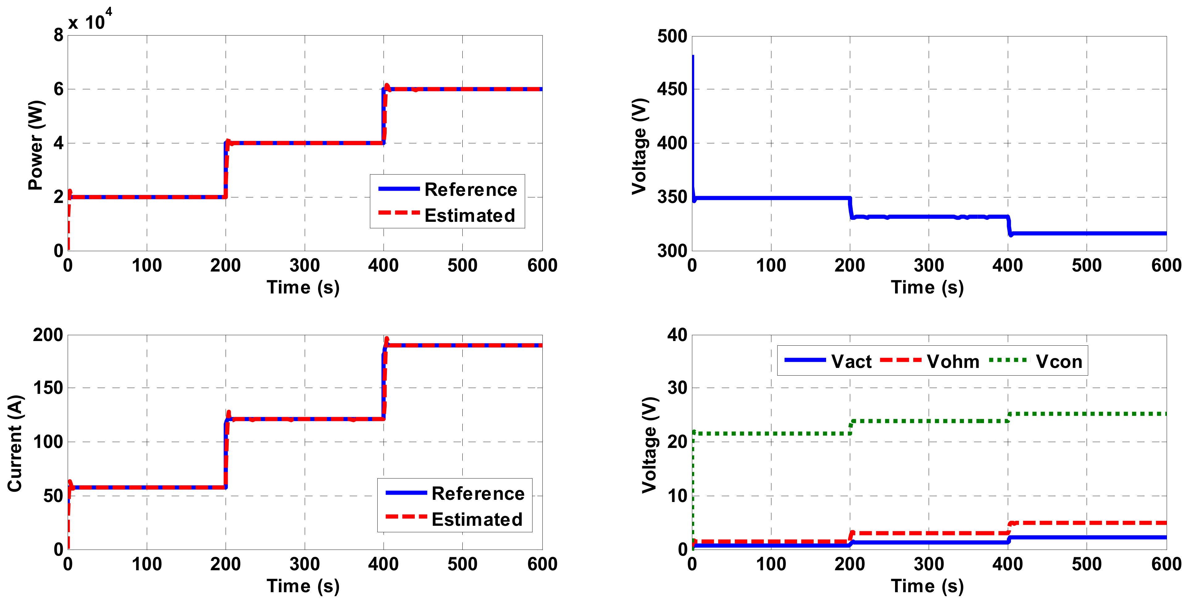
After identifying the parameters of the transient-state based model of SOFC, the model of fuel cell is implemented in Simulink/Matlab, and two load disturbances are applied to the model. The first disturbance is shown in Figure 10 (1st graph), the power is changed from 30 kW to 60 kW at a time of 300 sec., and given the identified parameters via the proposed EO and the stack output power plotted with the load disturbance, it is clear that they are closely matched, this means that the EO succeeded in extracting the correct parameters of the SOFC dynamic model. Moreover, the load current of the constructed model is closely converged to the disturbance current (3rd graph, Figure 10). Moreover, the terminal voltage (2nd graph) and the voltage drops occur inside the stack (4th graph), and they are shown in Figure 10. The constructed model via the proposed EO succeeded in tracking the changes in the load power. Moreover, a second disturbance is applied on the dynamic model in which the load power has two variations; as shown in Figure 11 (1st graph), the load power changes from 20 kW to 40 kW at 200 s and then changes again to 60 kW at 400 s on the same graph. The output power from the constructed model with identified parameters via the proposed EO is given, and both curves are converged. The terminal voltage, the corresponding current, and the voltage drops are shown in Figure 11 (2nd graph, 3rd graph, and 4th graph, respectively).

Finally, it can be concluded that the proposed methodology incorporating the EO is reliable, superior, and efficient over other employed approaches in constructing a reliable model of the SOFC-based model operated under either steady-state or dynamic-state modes.

6. Conclusions

This work introduces a new methodology based on a new metaheuristic approach named equilibrium optimizer (EO) to estimate the optimal parameters of a solid oxide fuel cell (SOFC) model. This is achieved with the aid of experimental datasets of the fuel cell polarization curves. The sum squared error difference between the cell experimental and computed voltages is selected as the fitness function to be minimized. The work investigates two operating modes of FC, which are steady- and dynamic-states models under altering operating conditions. In the first model, the parameters are estimated at four temperatures via the recorded measured polarization curves at them. In the dynamic model, two load power disturbances are investigated after identifying the parameters via the proposed EO. The obtained results via the proposed EO are compared to those obtained by the Archimedes optimization algorithm (AOA), Heap-based optimizer (HBO), Seagull Optimization Algorithm (SOA), Student Psychology Based Optimization Algorithm (SPBO), Marine predator algorithm (MPA), Manta ray foraging optimization (MRFO), and comprehensive learning dynamic multi-swarm marine predators algorithm. In the case of the SOFC steady-state model, the proposed EO succeeded in achieving the best (minimum) fitness function of 2.6906 × 10⁻⁶, 1.5527 × 10⁻⁶, 2.6809 × 10⁻⁶, and 2.2995 × 10⁻⁶ at operating temperature of 1073 K, 1173 K, 1213 K, and 1273 K, respectively. The corresponding standard deviations in the four studied cases obtained via the proposed EO are 9.15673 × 10⁻⁷, 1.63132 × 10⁻⁶, 3.36081 × 10⁻⁶, and 2.2119 × 10⁻⁶. Regarding the obtained results of the SOFC dynamic-state model, the proposed EO outperformed the others, achieving the minimum SMSE with a value of 1.0406; the MRFO comes in the second rank with a fitness function of 1.0775, and then the CLDMMPA achieves a SMSE of 1.3204 and comes in the third rank. The proposed EO succeeded in achieving a variance of 0.02264 and a standard deviation of 0.15048 in this studied case. The findings of this study demonstrate the superiority and reliability of the proposed approach in constructing a good-performance model that converges to the real one.

References

1. Capodaglio, A.G.; Cecconet, D.; Molognoni, D. An integrated mathematical model of microbial fuel cell processes: Bioelectrochemical and microbiologic aspects. Processes 2017, 5, 73. [Google Scholar] [CrossRef] [Green Version]
2. Bizon, N.; Thounthong, P. Energy efficiency and fuel economy of a fuel cell/renewable energy sources hybrid power system with the load-following control of the fueling regulators. Mathematics 2020, 8, 151. [Google Scholar] [CrossRef] [Green Version]
3. Wilberforce, T.; El-Hassan, Z.; Khatib, F.; Al Makky, A.; Baroutaji, A.; Carton, J.G.; Olabi, A.G. Developments of electric cars and fuel cell hydrogen electric cars. Int. J. Hydrogen Energy 2017, 42, 25695–25734. [Google Scholar] [CrossRef] [Green Version]
4. El-Hay, E.A.; El-Hameed, M.A.; El-Fergany, A.A. Performance enhancement of autonomous system comprising proton exchange membrane fuel cells and switched reluctance motor. Energy 2018, 163, 699–711. [Google Scholar] [CrossRef]
5. Rokni, M. Addressing fuel recycling in solid oxide fuel cell systems fed by alternative fuels. Energy 2017, 137, 1013–1025. [Google Scholar] [CrossRef] [Green Version]
6. Olabi, A. Renewable energy and energy storage systems. Energy 2017, 136, 1–6. [Google Scholar] [CrossRef]
7. Ramadhani, F.; Hussain, M.; Mokhlis, H.; Hajimolana, S. Optimization strategies for Solid Oxide Fuel Cell (SOFC) application: A literature survey. Renew. Sustain. Energy Rev. 2017, 76, 460–484. [Google Scholar] [CrossRef]
8. Chowdhury, S.; Chowdhury, S.P.; Crossley, P. Microgrids and Active Distribution Networks; The Institution of Engineering and Technology: London, UK, 2009. [Google Scholar]
9. El-Hay, E.; El-Hameed, M.; El-Fergany, A. Steady-state and dynamic models of solid oxide fuel cells based on Satin Bowerbird Optimizer. Int. J. Hydrogen Energy 2018, 43, 14751–14761. [Google Scholar] [CrossRef]
10. El-Hay, E.; El-Hameed, M.; El-Fergany, A. Optimized parameters of SOFC for steady state and transient simulations using interior search algorithm. Energy 2019, 166, 451–461. [Google Scholar] [CrossRef]
11. Van Biert, L.; Godjevac, M.; Visser, K.; Aravind, P. Dynamic modelling of a direct internal reforming solid oxide fuel cell stack based on single cell experiments. Appl. Energy 2019, 250, 976–990. [Google Scholar] [CrossRef]
12. Gong, W.; Yan, X.; Hu, C.; Wang, L.; Gao, L. Fast and accurate parameter extraction for different types of fuel cells with decomposition and nature-inspired optimization method. Energy Convers. Manag. 2018, 174, 913–921. [Google Scholar] [CrossRef]
13. Ettihir, K.; Boulon, L.; Becherif, M.; Agbossou, K.; Ramadan, H. Online identification of semi-empirical model parameters for PEMFCs. Int. J. Hydrogen Energy 2014, 39, 21165–21176. [Google Scholar] [CrossRef]
14. Ang, S.M.C.; Brett, D.J.; Fraga, E.S. A multi-objective optimisation model for a general polymer electrolyte membrane fuel cell system. J. Power Sources 2010, 195, 2754–2763. [Google Scholar] [CrossRef] [Green Version]
15. Tahmasbi, A.A.; Hoseini, A.; Roshandel, R. A new approach to multi-objective optimisation method in PEM fuel cell. Int. J. Sustain. Energy 2013, 34, 283–297. [Google Scholar] [CrossRef]
16. Petrescu, S.; Petre, C.; Costea, M.; Malancioiu, O.; Boriaru, N.; Dobrovicescu, A.; Feidt, M.; Harman, C.; Stanciu, C. A methodology of computation, design and optimization of solar Stirling power plant using hydrogen/oxygen fuel cells. Energy 2010, 35, 729–739. [Google Scholar] [CrossRef]
17. Virkar, A.; Williams, M.C.; Singhal, S. Concepts for ultra-high power density solid oxide fuel cells. ECS Trans. 2007, 5, 401–421. [Google Scholar] [CrossRef]
18. Zhu, L.; Zhang, L.; Virkar, A.V. A parametric model for solid oxide fuel cells based on measurements made on cell materials and components. J. Power Sources 2015, 291, 138–155. [Google Scholar] [CrossRef] [Green Version]
19. Shi, H.; Li, J.; Zafetti, N. New optimized technique for unknown parameters selection of SOFC using Converged Grass Fibrous Root Optimization Algorithm. Energy Rep. 2020, 6, 1428–1437. [Google Scholar] [CrossRef]
20. Yousri, D.; Hasanien, H.M.; Fathy, A. Parameters identification of solid oxide fuel cell for static and dynamic simulation using comprehensive learning dynamic multi-swarm marine predators algorithm. Energy Convers. Manag. 2021, 228, 113692. [Google Scholar] [CrossRef]
21. Nassef, A.M.; Fathy, A.; Sayed, E.T.; Abdelkareem, M.A.; Rezk, H.; Tanveer, W.H.; Olabi, A. Maximizing SOFC performance through optimal parameters identification by modern optimization algorithms. Renew. Energy 2019, 138, 458–464. [Google Scholar] [CrossRef]
22. Fathy, A.; Rezk, H.; Ramadan, H.S.M. Recent moth-flame optimizer for enhanced solid oxide fuel cell output power via optimal parameters extraction process. Energy 2020, 207, 118326. [Google Scholar] [CrossRef]
23. Wang, X.; Huang, B.; Chen, T. Data-driven predictive control for solid oxide fuel cells. J. Process. Control 2007, 17, 103–114. [Google Scholar] [CrossRef]
24. Larminie, J.; Dicks, A.; McDonald, M.S. Fuel Cell Systems Explained; John Wiley & Sons: Chichester, UK, 2003; Volume 2. [Google Scholar]
25. Faramarzi, A.; Heidarinejad, M.; Stephens, B.; Mirjalili, S. Equilibrium optimizer: A novel optimization algorithm. Knowl. Based Syst. 2020, 191, 105190. [Google Scholar] [CrossRef]
26. Wei, Z.; Zou, C.; Leng, F.; Soong, B.H.; Tseng, K.-J. Online model identification and state-of-charge estimate for lithium-ion battery with a recursive total least squares-based observer. IEEE Trans. Ind. Electron. 2018, 65, 1336–1346. [Google Scholar] [CrossRef]
27. Wei, Z.; Zhao, J.; Xiong, R.; Dong, G.; Pou, J.; Tseng, K.J. Online estimation of power capacity with noise effect attenuation for lithium-ion battery. IEEE Trans. Ind. Electron. 2019, 66, 5724–5735. [Google Scholar] [CrossRef]
28. Wei, Z.; Zhao, D.; He, H.; Cao, W.; Dong, G. A noise-tolerant model parameterization method for lithium-ion battery management system. Appl. Energy 2020, 268, 114932. [Google Scholar] [CrossRef]
29. Wei, Z.; Meng, S.; Xiong, B.; Ji, D.; Tseng, K.J. Enhanced online model identification and state of charge estimation for lithium-ion battery with a FBCRLS based observer. Appl. Energy 2016, 181, 332–341. [Google Scholar] [CrossRef]
30. Pierre, J. Siemens energy. In Proceedings of the 11th Annual SECA Workshop, Pittsburgh, PA, USA, 27–29 July 2010. [Google Scholar]
31. Xu, D.; Jiang, B.; Liu, F. Improved data driven model free adaptive constrained control for a solid oxide fuel cell. IET Control. Theory Appl. 2016, 10, 1412–1419. [Google Scholar] [CrossRef]
Figure 1. Optimization process of EO.
Mathematics 09 01066 g001
Figure 2. The proposed steps incorporating EO.
Mathematics 09 01066 g002
Figure 3. The measured and calculated polarization curves of SOFC operated at 1073 K obtained via EO at (a) current density-voltage, (b) current density-power.
Mathematics 09 01066 g003
Figure 4. (a) Current-voltage curve, (b) Current-power curve of SOFC operated at 1073 K obtained via other approaches.
Mathematics 09 01066 g004
Figure 5. The variation of fitness function during iterative process for all employed optimizers applied for steady-state SOFC model.
Mathematics 09 01066 g005
Figure 6. The measured and calculated (a) current density-voltage, (b) current density-power of SOFC operated at 1173 K, 1213 K, and 1273 K obtained via the proposed EO.
Mathematics 09 01066 g006
Figure 7. The measured and calculated polarization curves of SOFC dynamic-state model operated at 1273 K obtained via EO (a) current-voltage, (b) current-power.
Mathematics 09 01066 g007
Figure 8. The measured and calculated polarization curves of SOFC dynamic-state model operated at 1273 K obtained via MPA, HBO, SOA, and MRFO.
Mathematics 09 01066 g008
Figure 9. The variation of fitness function during iterative process for all employed optimizers applied for dynamic-state SOFC model.
Mathematics 09 01066 g009
Figure 10. First load disturbance applied on SOFC stack dynamic model.
Mathematics 09 01066 g010
Figure 11. Second load disturbance applied on SOFC stack dynamic model.
Mathematics 09 01066 g011