Development of a Backward–Forward Stochastic Particle Tracking Model for Identification of Probable Sedimentation Sources in Open Channel Flow

Abstract

As reservoirs subject to sedimentation, the dam gradually loses its ability to store water. The identification of the sources of deposited sediments is an effective and efficient means of tackling sedimentation problems. A state-of-the-art Lagrangian stochastic particle tracking model with backward–forward tracking methods is applied to identify the probable source regions of deposited sediments. An influence function is introduced into the models to represent the influence of a particular upstream area on the sediment deposition area. One can then verify if a specific area might be a probable source by cross-checking the values of influence functions calculated backward and forward, respectively. In these models, the probable sources of the deposited sediments are considered to be in a grid instead of at a point for derivation of the values of influence functions. The sediment concentrations in upstream regions must be known a priori to determine the influence functions. In addition, the accuracy of the different types of diffusivity at the water surface is discussed in the study. According to the results of the case study of source identification, the regions with higher sediment concentrations computed by only backward simulations do not necessarily imply a higher likelihood of sources. It is also shown that from the ensemble results when the ensemble mean of the concentration is higher, the ensemble standard deviation of the concentration is also increased.

1. Introduction

Sediment that is trapped behind dams reduces reservoir capacity. In some high-profile cases reservoirs have been found to be filled with sediment, not only worsening their functions and/or rendering a weakened dam infrastructure, but also posing a safety hazard [1,2,3,4]. Despite more than six decades of research, sedimentation remains probably the most serious technical problem faced by the dam industry, and sedimentation in reservoirs is now of primary global importance [5]. To study reservoir sedimentation, adequate knowledge of the sediment transport process in rivers is needed [6].

According to the Taiwan Water Resources Agency [7], most riverbeds and banks in Taiwan are prone to erosion, resulting in high sediment concentrations in most rivers. When sediment particles in a river are transported to a reservoir, the flow velocity is reduced and thus a larger volume of sediment particles is deposited at the bottom of the reservoir, which is a process referred to as reservoir sedimentation. The Shihmen reservoir, located in Taoyuan, is one of the main reservoirs in northern Taiwan. It provides domestic as well as agricultural water supply and hydroelectricity for more than three million people in northern Taiwan. In addition, the Shihmen reservoir also plays the role as a detention basin for the Taipei Basin. It has an effective storage capacity of nearly 309 million cubic meters, of which the sediment has occupied 31.6% since 2009 [7]. Sedimentation is one of the most important engineering problems that threaten reservoirs around the world. Traditionally, dredging and sluicing are passive methods, which cannot completely resolve the sedimentation problem since the sediment particles are deposited continuously during the removal process [8]. To manage reservoirs in a more sustainable way, identifying the source of the sediment particles is one step toward dealing with the problem [4].

Sediment-related issues can be prevented in advance when the probable sources of these deposited sediments are identified and prevented from flowing into the reservoirs. The turbulent characteristics of open channel flows are important in understanding particle transport phenomena, which consist of highly disordered and chaotic fluid motions over a wide range of length scales and frequencies [9,10,11,12,13,14,15,16,17]. This study examines the probable source regions of deposited sediments using a Backward–Forward Stochastic Diffusion Particle Tracking Model (Backward–Forward SD-PTM), a method of Lagrangian dynamics [18]. Not only the particle concentrations but also the particle trajectories can be simulated.

The stochastic diffusion particle tracking model (SD-PTM) is intrinsically irreversible owing to its stochastic nature. Some investigations have implied that the results of backward tracking can provide valuable clues about the probable sources of deposited sediments [19]. The probable sources are determined not only by the backward tracking process but also by the forward tracking process. Therefore, although most partial differential equations cannot be solved reversibly such as by finding the initial conditions from the results, the places of probable sources (herein considered as initial conditions) can still be identified, thus providing valuable information for solving sedimentation problems [19].

In the SD-PTM, a Brownian motion term describes the randomness of particle motion. The probability distribution of particle positions or particle concentrations can thus be computed by performing sufficient simulation runs of a single particle, or by a single simulation run with many independent particles. Notably, the distribution of the concentrations may vary among simulations. Consequently, an attempt is made herein to simulate such distribution multiple times to acquire a more accurate concentration distribution.

The objectives of this study are threefold. First, we aim to identify the probable source of deposited particles using the backward SD-PTM, and the forward SD-PTM, respectively. Next, we intend to develop a complete backward–forward particle tracking model. We then aim at enhancing the accuracy issue of estimating diffusivity coefficients when a particle has reached the water surface. Lastly, we improve the accuracy of the concentration distribution of sediment particles by computing the ensemble statistics of concentration distributions.

In Section 2, literature about the SD-PTM, backward–forward SD-PTM will be reviewed. In Section 3, some case studies applying backward SD-PTM or forward SD-PTM will be discussed. The influence function, a quantitative link between each source-receptor pair, is introduced in Section 4. Then, the model established in Section 4 will be applied in Section 5 to illustrate how to identify probable sources with the explicit and the implicit methods, respectively. In Section 6, more scenarios of the spatial sediment concentration distributions are concerned in a case study applying the backward–forward SD-PTM to identify probable sources. In Section 7, some conclusions and recommendations will be provided.

2. Methodologies

2.1. Stochastic Particle Tracking Model

Recently, in the field of sediment transport, particle-based approaches for estimating mass concentrations or concentrations of soil particles in a tidal estuary have been developed [20,21,22,23,24]. Man and Tsai [25] later presented an SD-PTM to simulate the trajectories of sediment particles in open channel flows. An SDE is a differential equation that includes at least one stochastic process term. For example, the stochastic process term can be presented as a derivative of Brownian motion or a Wiener process as follows:

$$d{\mathit{X}}_{\mathit{t}}=\mathit{f}\left({\mathit{X}}_{\mathit{t}},t\right)dt+\mathit{g}\left({\mathit{X}}_{\mathit{t}},t\right)d\mathit{W}$$

(1)

In Equation (1), $d{\mathit{X}}_{\mathit{t}}$, $\mathit{f}\left({\mathit{X}}_{\mathit{t}},t\right)$, $\mathit{g}\left({\mathit{X}}_{\mathit{t}},t\right)$, $d\mathit{W}$ represent a stochastic process, deterministic drift term, the size of the fluctuation of the stochastic term and a standard Wiener process, respectively. Note that boldface type symbols denote vector or matrix quantities in this paper. According to Man et al. [25], $\mathit{f}\left({\mathit{X}}_{\mathit{t}},t\right)=\overline{\mathit{u}}\left({\mathit{X}}_{\mathit{t}},t\right)=\overline{\mathit{U}}+\nabla \mathit{D}$. Moreover, the size of the uncertain movement of sediment particles caused by turbulence is assumed to be proportional to the diffusion coefficient $\mathit{\sigma }$. $\mathit{g}\left({\mathit{X}}_{\mathit{t}},t\right)=\mathit{\sigma }\left({\mathit{X}}_{\mathit{t}},t\right)$ can then be obtained. Numerically, $d\mathit{W}$ can be simulated as a normally distributed random variable $\mathit{N}\left(0,\sqrt{dt}\right)$ with mean zero and variance $dt$, where $dt$ is the time step for numerical simulation. Therefore, the governing equation in the numerical form of the SD-PTM can be written as follows:

$${\mathit{X}}_{\mathit{n}+\mathit{1}}={\mathit{X}}_{\mathit{n}}+\overline{\mathit{u}}\left({\mathit{X}}_{\mathit{n}},t\right)dt+\mathit{\sigma }\left({\mathit{X}}_{\mathit{n}},t\right)\mathit{N}\left(0,\sqrt{dt}\right)$$

(2)

The SD-PTM, composed of both a mean drift term and a random term, is capable of capturing any randomly selected scenarios of particle movement. Equation (2) can be coupled with a re-suspension process to simulate the movement of suspended sediment particles.

Oh and Tsai [26] added a jump term to the SD-PTM to simulate perturbation by randomly occurring extreme events including sediment deposition and re-suspension. Subsequently, Tsai et al. [27] introduced several particle tracking models to describe particle movement under various flow conditions, i.e., the stochastic diffusion process, stochastic jump process, and stochastic jump-diffusion process. Tsai et al. [24] concentrated on the jump term in the stochastic particle tracking model by studying the influence on sediment movement of the frequency and change in the magnitude of extreme events.

Oh et al. [28] suggested using the spatial distribution of particles to estimate sediment concentration and found that a high concentration is associated with a high ensemble standard deviation. Tsai et al. [29] coupled the random arrival process of particles with the SD-PTM to simulate the trajectories of sediment particles. Oh et al. [30] examined the longitudinal distance between pairs of sediment particles using the SD-PTM model. They found that a smaller particle and a higher release point leads to a longer average travel distance to the particle deposition point.

2.2. Backward–Forward Stochastic Particle Tracking Model

The usage of backward simulations is to reduce the CPU time required to run a Monte Carlo simulation for estimating particle concentrations. Spivakovskaya et al. [31] applied a forward–reverse particle tracking system that the Monte Carlo estimator for the particle concentration can also be based on. The results show that the CPU time is reduced by at least an order of magnitude compared with the classical Monte Carlo method.

Lin et al. [32]. introduced the Stochastic Time-Inverted Lagrangian Transport (STILT) model of atmospheric transport, which can be used to map the upstream influence (the probable source region) of the particle deposition point (the receptor). Lin et al. [32] were concerned with preventing inconsistencies in the backward and forward simulations of the time evolution of a particle ensemble using the STILT model. That is to say, they removed apparently irreversible particle trajectories, as can be done with the help of the “influence function,” which was first proposed by Uliasz and Pielke [33]. The influence function is a quantitative indicator of a source’s influence on a receptor at which a tracer particle is observed:

$$I\left(x_r,t_r|x,t\right)=\frac{1}{N_{tot}}{\displaystyle \sum }_{i=1}^{N_{tot}}\delta \left(x_i\left(p\right)-x\right)$$

(3)

The influence function $I\left(x_r,t_r|x,t\right)$ denotes the influence of an upstream source at $x$ at time $t$ on a downstream receptor at $x_r$ at time $t_r$. The delta function $\delta \left(x_i\left(p\right)-x\right)$ represents whether the particle appears in the source. $N_{tot}$ is the total number of particles that are released at a source.

Seibert and Frank [34] also applied the linear source-receptor relationship in the backward Lagrangian particle dispersion model (LPDM) for atmospheric particles. They found that the LPDM, combined with backward simulations, is an effective tool for making point measurements, which can be handled without artificial numerical diffusion. Subsequently, Batchelder [18] employed Forward-in-Time-Trajectory/Backward-in-Time-Trajectory (FITT/BITT) modeling to identify sources of ocean organisms, such as plankton. Their research showed that the BITT approach combined with the FITT approach is more efficient in locating sources of particles than the simulations using only the FITT approach. Isobe et al. [19] later developed a method that involved backward- and forward-random walk processes for identifying the sources of particles that drift on an ocean surface. They argued that although the random walk process is irreversible, it provides valuable information when the duration of the simulation is relatively short. They found some potential probable source regions by backward-in-time simulations. The authors presented a case study of East China Sea, and statistically significant sources are well specified close to the true source since 58% to 90% of source candidates are rejected experimentally.

Most current research on backward particle tracking models is in the field of atmospheric science or ocean science. However, few investigations of backward sediment transport in an open channel can be found. Hence, the behaviors of sediments in stochastic backward particle tracking processes are of interest. In this study, some backward tracking approaches that involve the SD-PTM are used to provide some hints to the identities of probable sources of sedimentation.

3. Case Studies of Backward or Forward SD-PTM

In this section, the flow conditions and particle parameters are adopted from the experimental data by Kaftori et al. [35], which studied the behavior of particles in the wall region of a turbulent boundary layer. The SD-PTM is applied to simulate sediment transport in open channel flow. A vast number of random scenarios of particle trajectories are modeled using SD-PTM. Then, by performing Monte Carlo simulations, the ensemble means and ensemble variances of particle positions can be analyzed.

3.1. Model Setup

The simulation is conducted on two dimensions, which are the stream-wise direction (x) and the gravitational direction (z). In the stream-wise direction, the drift term dominates the particle velocity. Therefore, the diffusivity and turbulence terms can be ignored. In the stream-wise direction, the drift flow velocity is assumed to follow the logarithm profile, consistent with Equation (4).

$$\frac{\overline{u}}{u_{\ast }}=\frac{1}{\kappa }ln\left(\frac{30z}{k_s}\right)$$

(4)

The mean drift flow velocity in the x-direction is a function of z. $u_{\ast }$ is the shear velocity and $k_s$ is the roughness height. When the above assumptions are taken into consideration, the numerical governing Equation (2) for forward tracking in the x-direction can be written as follows.

$$X_{n+1}=X_n+\frac{u_{\ast }}{\kappa } ln\left(\frac{30Z_n}{k_s}\right)dt$$

(5)

The numerical governing Equation (2) for forward tracking in the z-direction can be written as follows. The turbulence diffusivity in the z-direction $D_z$ is a function of position $z_n$, and $w_s$ is the settling velocity.

$$Z_{n+1}=Z_n+\left(\overline{W_n}-w_s+\frac{\partial D_z\left(Z_n\right)}{\partial z}\right)dt+\sqrt{2D_z\left(Z_n\right)}\mathrm{N}\left(0,\sqrt{dt}\right)$$

(6)

When a particle is transported to the bed, re-suspension may occur by the mechanisms that were proposed by Wu and Lin [36], who suggested that a log-normal distribution of instantaneous velocities $u_b$ outperforms a normal distribution of $u_b$ in approaching particles on the bed when considering the pickup probability threshold. According to Wu et al. [36], the threshold $B$ is shown below.

$$lnB=ln\left(\sqrt{4Di\left({\rho }_s-\rho \right)g/\left(3\rho C_L\right)}\right)$$

(7)

In Equation (7), $Di$, ${\rho }_s$, $\rho$, $g$, $C_L$ represent particle diameter, particle density, water density, gravity acceleration, and lift coefficient respectively.

3.2. Model Parameters

In this study, the formula proposed by Rouse [37] or by Absi et al. [38] is adopted in calculating turbulence diffusivity. Rouse [37] proposed the following vertical kinematic viscosity of a fluid:

$$D_z=\kappa u_{\ast }Z\left(1-\frac{Z}{H}\right)$$

(8)

$D_z$, $u_{\ast }$, $Z$, $H$ represent turbulence diffusivity in the z-direction, the shear velocity, the z-coordinate of particle position, and the flow depth respectively.

If Rouse’s diffusivity is adopted, then the numerical governing equation in the z-direction for forward tracking can be written as follows:

$$Z_{n+1}=Z_n+\left(\overline{W_n}-w_s+\kappa u_{\ast }-2\kappa u_{\ast }\frac{Z_n}{H}\right)dt+\sqrt{2\kappa u_{\ast }{Z}_n\left(1-\frac{Z_n}{H}\right)}\mathrm{N}\left(0,\sqrt{dt}\right)$$

(9)

Absi et al. [38] proposed the following formula for the diffusivity of suspended particles.

$$D_z=\left(\frac{1}{1+St\left(Z\right)}+St\left(Z\right)\frac{\overline{v_y{}^{\prime }{}^2}}{\overline{u_y{}^{\prime }{}^2}}\right){\nu }_t\left(Z\right)$$

(10)

where $St\left(Z\right)$ is particle Stokes number, ${\nu }_t$ is eddy viscosity, and $k\left(Z\right)$ is turbulent kinetic energy. Turbulence intensities in the fluid phase and the solid phase are denoted as $\overline{u_y{}^{\prime }{}^2}$ and $\overline{v_y{}^{\prime }{}^2}$, respectively. The ratio of $\overline{u_y{}^{\prime }{}^2}$ to $\overline{v_y{}^{\prime }{}^2}$ is assumed to be $1-{\rho }_f/{\rho }_p$. The formulas for $St\left(Z\right)$, ${\nu }_t\left(Z\right)$ and $k\left(Z\right)$ are listed below.

$$St=\frac{w_s}{\left(1-\frac{{\rho }_f}{{\rho }_s}\right)g}\frac{k}{{\alpha }_0{\nu }_t}$$

(11)

$$k=u_{\ast }{}^2\frac{1}{C_{\mu }{}^2}exp\left[-\frac{\frac{Z{u}_{\ast }}{\nu }-a_k{}^{+}}{A_k{}^{+}}\right]$$

(12)

$${\nu }_t=Z{u}_{\ast }exp\left[-\frac{\frac{Z{u}_{\ast }}{\nu }+a_{\nu }{}^{+}}{A_{\nu }{}^{+}}\right]$$

(13)

where $C_{\mu }=$ 0.09, ${\alpha }_0$=$1/C_{\mu }$, and $a_k{}^{+}$, $A_k{}^{+}$, $a_{\nu }{}^{+}$ and $A_{\nu }{}^{+}$ are friction-Reynolds-number-dependent parameters.

3.3. Case Studies of Backward Tracking with Rouse’s Diffusivity Coefficients

In this section, the diffusivity formula adopted is Rouse’s diffusivity formula. Thus, the governing equations in the x- and z-directions are derived from Equations (5) and (9) respectively. The particle parameters, initial conditions, channel settings, and simulation parameters are presented in

Table 1. Particles, initial conditions, flow conditions, and simulation parameters for backward and forward tracking tests.

Parameter	Unit	Value
		Backward Tracking Test	Forward Tracking Test
Diameter ($D_i$)	$\mathrm{m}$	$275\times {10}^{-6}$	$275\times {10}^{-6}$
Density (${\rho }_s$)	$\mathrm{k}\mathrm{g}/{\mathrm{m}}^3$	$1050$	$1050$
Lift coefficient ($C_L$)		$0.21$	$0.21$
Shear velocity ($u_{\ast }$)	$\mathrm{m}/\mathrm{s}$	$0.0086$	$0.0086$
Settling velocity ($w_s$)	$\mathrm{m}/\mathrm{s}$	$0.0025$	$0.0025$
Reference height ($z_b$)	$\mathrm{m}$	$275\times {10}^{-6}$	$275\times {10}^{-6}$
Roughness height ($ks$)	$\mathrm{m}$	$275\times {10}^{-6}$	$275\times {10}^{-6}$
$\mathrm{Initial} \mathrm{position} (x_0)$	$\mathrm{m}$	0	−1.5
$\mathrm{Initial} \mathrm{position} \left(z_0\right)$	$\mathrm{m}$	$275\times {10}^{-6}$	0.0284
Flow depth (H)	$\mathrm{m}$	0.0284	0.0284
Mean drift flow velocity $(\overline{w}$)	$\mathrm{m}/\mathrm{s}$	0	0
Time step ($dt$)	$\mathrm{s}$	0.01	0.01
Simulation Time ($T$)	$\mathrm{s}$	10	10
Number of simulations ($n$)		10,000	10,000

.

3.3.1. Explicit Method

Based on SD-PTM and the assumption that the timescale is small enough to enable the limit of the difference quotient of the governing equation to be properly estimated, the backward SD-PTM is developed by converting the operators of the numerical Lagrangian equations. This approach can be thought of as applying a negative velocity to a particle to obtain its previous location. In the explicit method, replacing the $Z_n$ on the right-hand sides of SDEs, Equations (5) and (9), with $Z_{n+1}$ and vice versa on the left-hand side, yields the following equations:

$$X_n=X_{n+1}-\frac{u_{\ast }}{\kappa }\kappa ln\left(\frac{30Z_{n+1}}{k_s}\right)dt$$

(14)

$$Z_n=Z_{n+1}-\left(\overline{W_n}-w_s+\kappa u_{\ast }-2\kappa u_{\ast }\frac{Z_{n+1}}{H}\right)\mathsf{\Delta }t-\sqrt{2\left(\kappa u_{\ast }{Z}_{n+1}\left(1-\frac{Z_{n+1}}{H}\right)\right)}N\left(0,\sqrt{dt}\right)$$

(15)

3.3.2. Implicit Method

The numerical Equations (5) and (9) can be rewritten as follows:

$$X_n=X_{n+1}-\frac{u_{\ast }}{\kappa }\kappa ln\left(\frac{30Z_n}{k_s}\right)dt$$

(16)

$$Z_n=Z_{n+1}-\left(\overline{W_n}-w_s+\kappa u_{\ast }-2\kappa u_{\ast }\frac{Z_n}{H}\right)dt-\sqrt{2\kappa u_{\ast }{Z}_n\left(1-\frac{Z_n}{H}\right)}N\left(0,\sqrt{dt}\right)$$

(17)

During the backward tracking process, each $Z_n$ is derived from a known $Z_{n+1}$. Accordingly, $Z_n$ can be regarded as an unknown variable while $Z_{n+1}$ is known. Thus, the numerical expression is implicit because the unknown $Z_n$ cannot be directly calculated.

If $A=\left[Z_{n+1}-\left(\overline{W_n}-w_s+\kappa u_{\ast }\right)dt\right]/\mathrm{N}\left(0,\sqrt{dt}\right)$, $B=\left(\frac{2\kappa u_{\ast }}{H}dt-1\right)/\mathrm{N}\left(0,\sqrt{dt}\right)$, $C=2\kappa u_{\ast }$ and $D=2\kappa u_{\ast }/H$, by squaring both sizes of Equation (17), yields a quadratic equation in $Z_n$:

$$\left(B^2+D\right)Z_n{}^2+\left(2AB-C\right)Z_n+A^2=0$$

(18)

Then $Z_n$ can be represented as follows.

$$Z_n=\left(C-2AB\right)\pm \sqrt{C^2-4ABC-4A^{2}D}/2\left(B^2+D\right)$$

(19)

Notably, the backward tracking process remains a stochastic process because the $\mathrm{N}\left(0,\sqrt{dt}\right)$ term is included in parameters $A$ and $B$. By the Taylor expansion of Equation (19), $Z_n$ is given by the following formula:

$$Z_n=\frac{Z_{n+1}-\left[f\left(Z_{n+1}, t_{n+1}\right)+Z_{n+1}{f}^{\prime }\left(Z_{n+1}, t_{n+1}\right)\right] \mathsf{\Delta }t}{1-f^{\prime }\left(Z_{n+1}, t_{n+1}\right)\mathsf{\Delta }t}$$

(20)

$f\left(Z_n, t_n\right)$ in Equation (20) is defined in Equation (21) as follow:

$$f\left(Z_n, t_n\right)= \left(\overline{W_n}-w_s+\frac{\partial D_z\left(Z_n\right)}{\partial z}\right)dt+\sqrt{2D_z\left(Z_n\right)}d{B}_t$$

(21)

Therefore, implicit numerical governing equations are derived as Equations (16) and (20).

3.4. Case Studies of Backward Tracking with Absi et al.’s Diffusivity Coefficients

The previous version of the model with diffusivity coefficients that were estimated using Rouse’s formula had a fundamental problem: it provided limited information about the particle position in the z-direction when a particle had reached the water surface. When $z=h$, the diffusion coefficient and the turbulence term would be zero (Equation (9)). Hence, particles remained at the surface once they had reached it in a natural system. Therefore, the accuracy of diffusivity coefficients is improved in this section by adopting the diffusivity proposed by Absi et al. [38]. In both explicit and implicit methods, the numerical governing equations are very similar to those in Section 3.3. The non-zero value of the diffusivity of Absi et al. [38] provides a means of tracking particles in the z-direction after they have reached the surface. Furthermore, since the formula of Absi et al. [38] considers the lag between fluid particles and sediment particles, diffusivity coefficients in this version may be more appropriate than the previous version using Rouse’s formula.

3.5. Comparison among Backward and Forward Tracking Cases

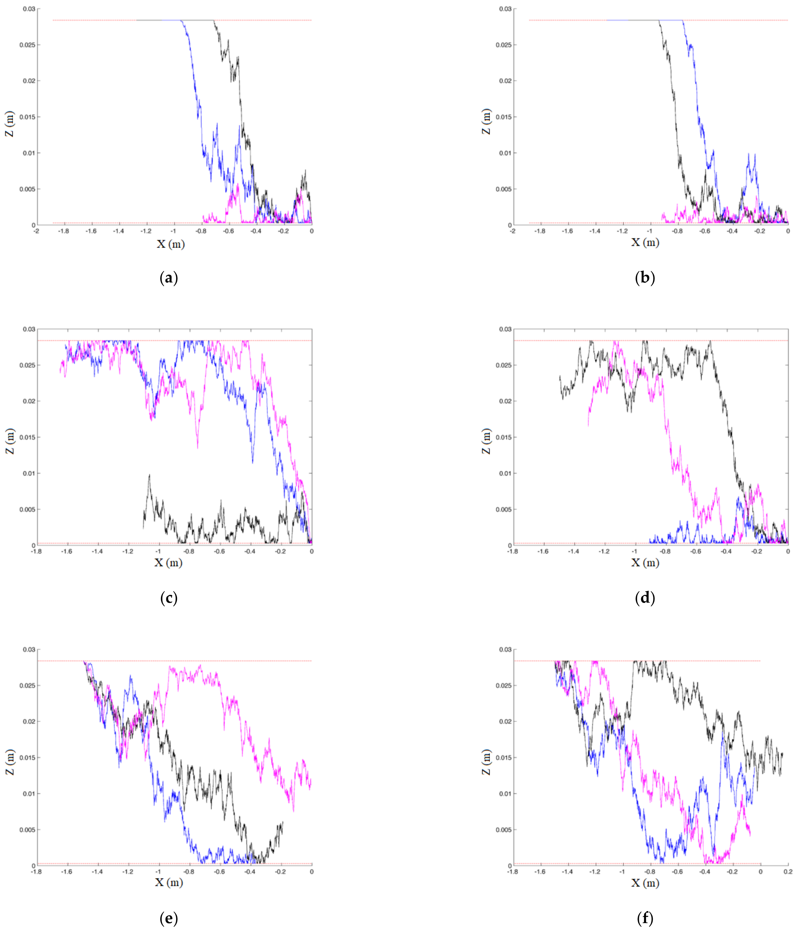
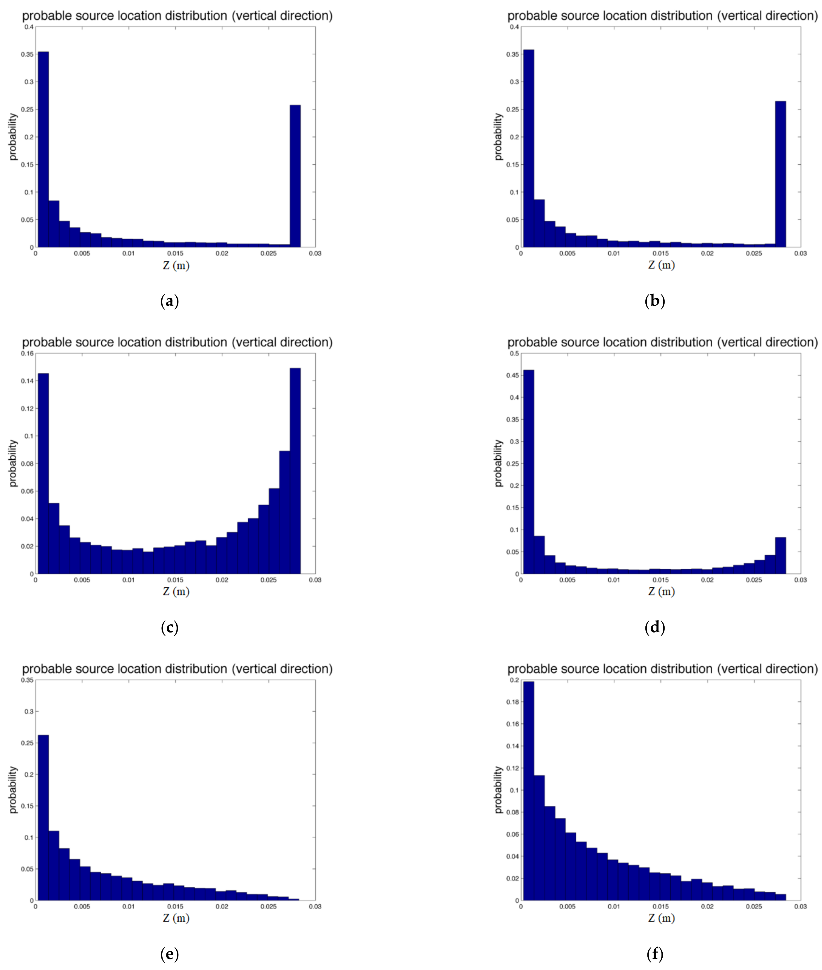
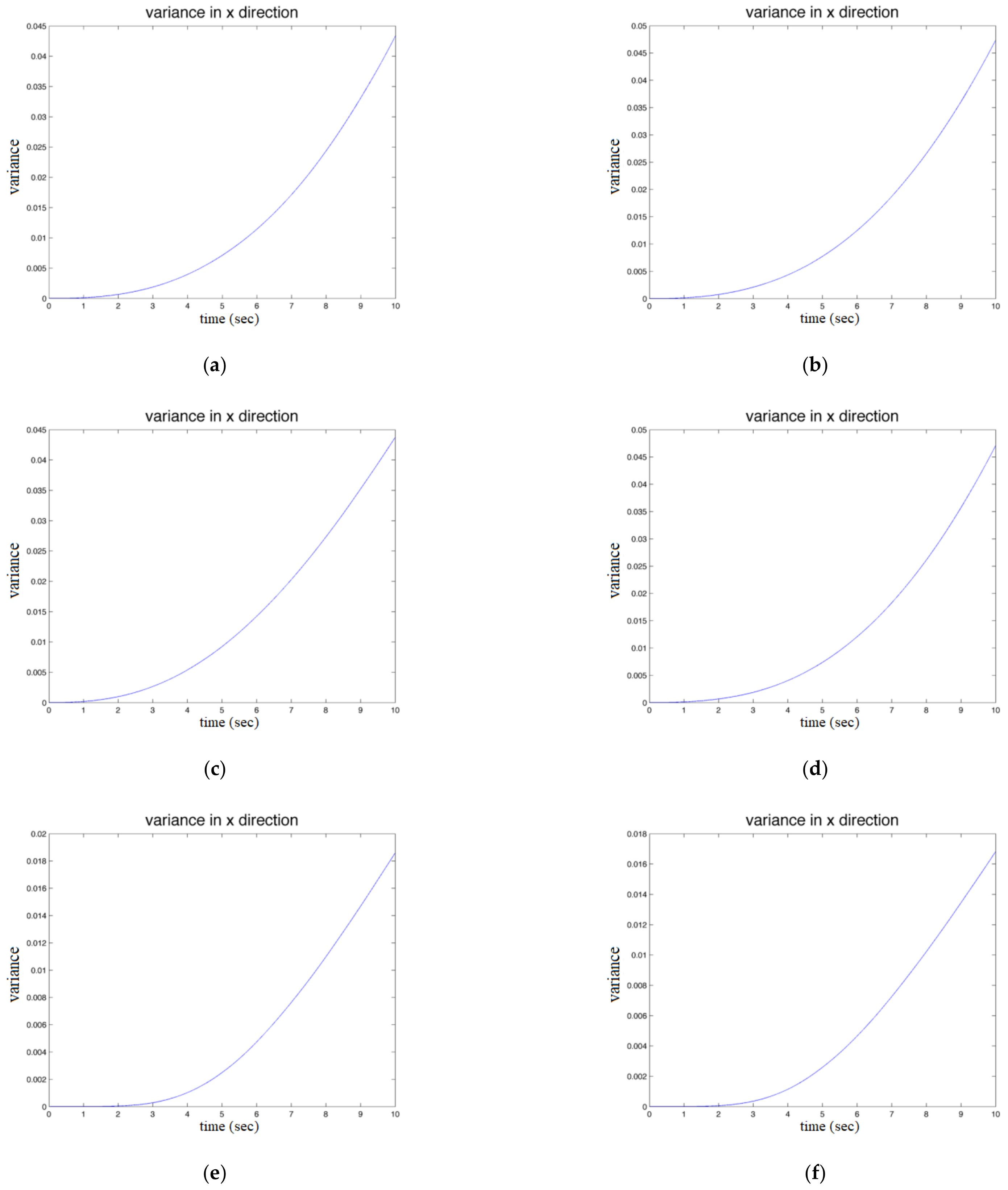
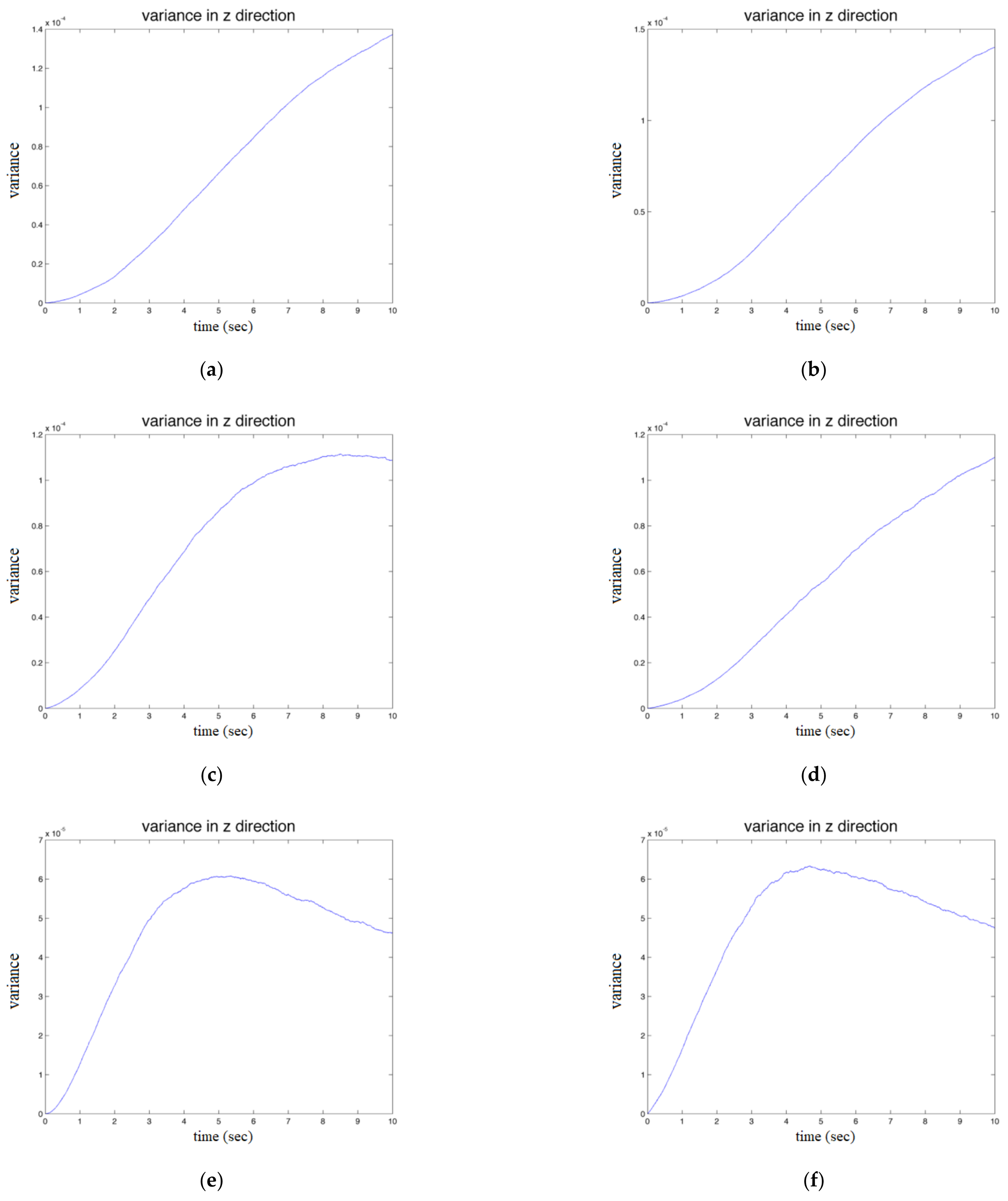
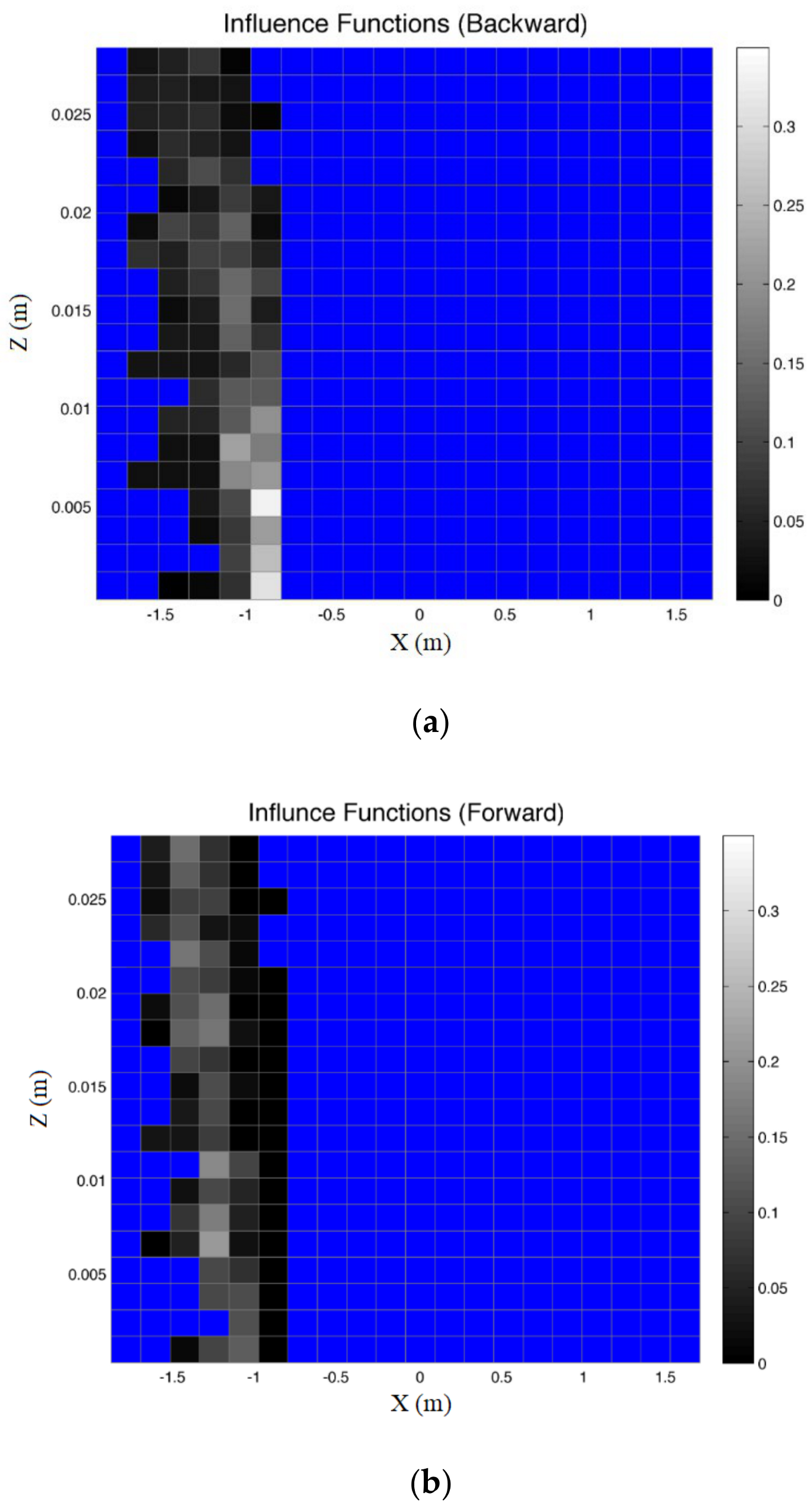
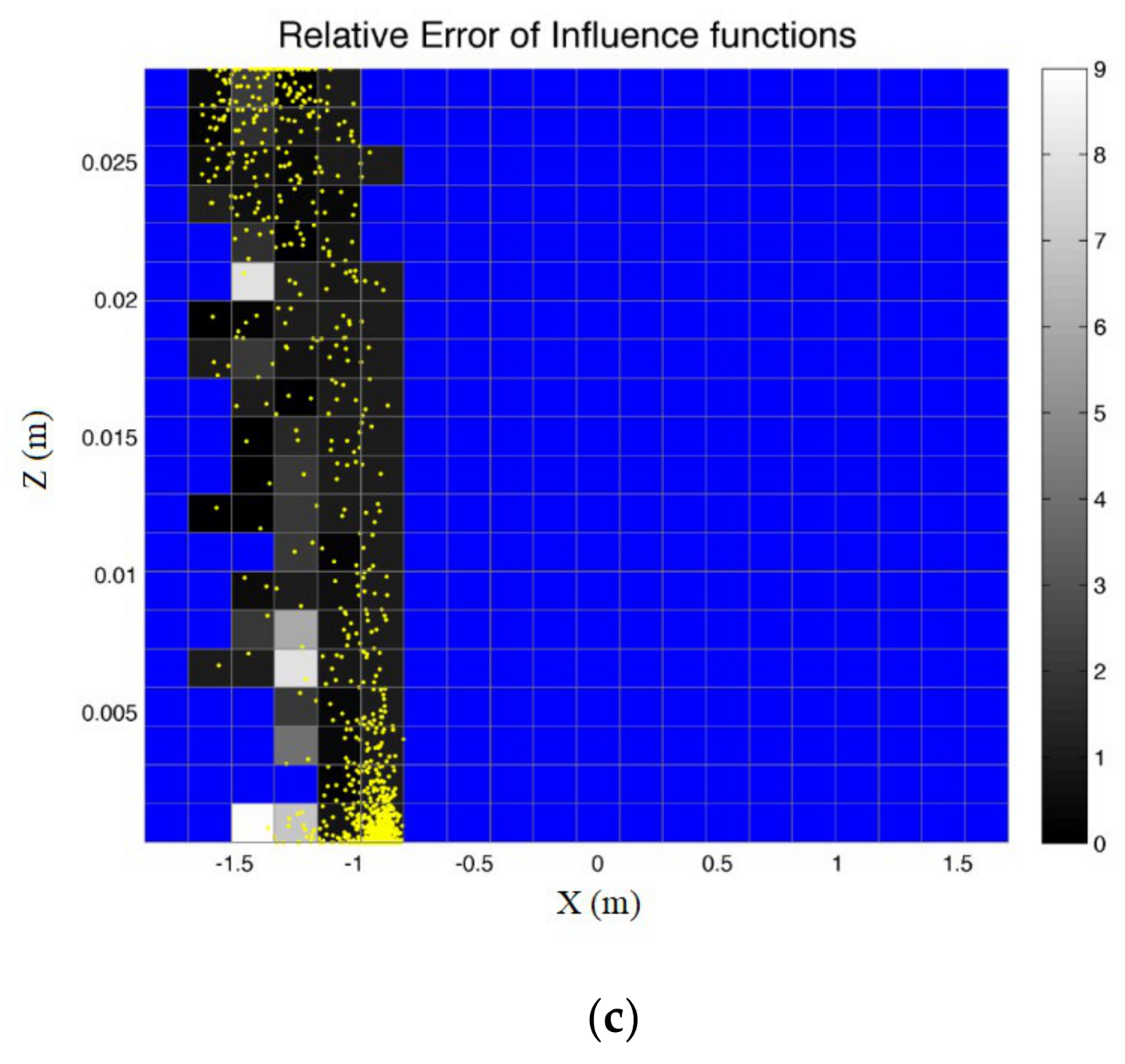
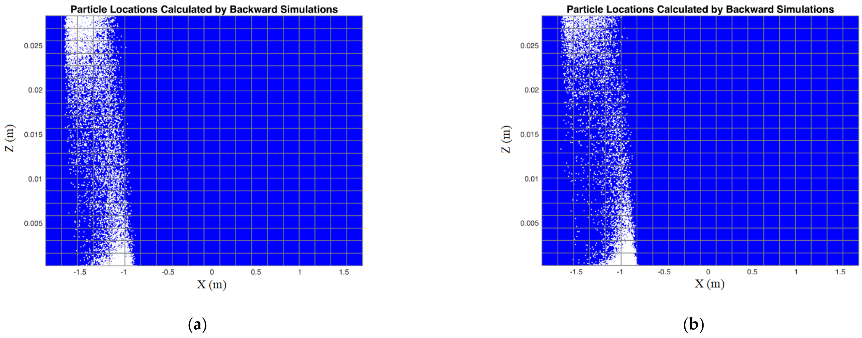
Additional to backward tracking, forward tracking is also exerted in Section 3. Figure 1, Figure 2, Figure 3, Figure 4, Figure 5, Figure 6 and Figure 7 present the results of simulations that involved scenarios, ensemble means of trajectories, probable source locations, and the distributions of probable source locations in both stream-wise and vertical directions. In those figures, a and b show backward tracking tests with the Rouse diffusivity, performed using the explicit and implicit method respectively; c and d represent backward tracking tests with the diffusivity of Absi et al. [38], conducted using the explicit and implicit method respectively; e and f show forward tracking tests carried out using the explicit method with the diffusivity of Rouse [37] and Absi et al. [38] respectively. In Figure 1 and Figure 2, the red line represents the water surface at z = 0.0284 (m).

According to Visser [39], though, the diffusivity should be evaluated at a slightly different location from $X_n$ for self-consistency of the process. In this section, we focus on the comparisons between diffusivities calculated by the functions of Rouse [37] and Absi et al. [38]. Therefore, we adopt the suggestion of Ross and Sharples [40], which is to output the particle positions of each time step to observe the difference between the aforementioned two numerical methods. It is shown in Figure 1a,b that particles would remain at the water surface once they reach the water surface due to the zero-vertical diffusivity of Rouse [37] at the water surface. However, this limitation can be eliminated with the diffusivity of Absi et al. [38]. From Figure 1b,c, the scenarios with the diffusivity of Absi et al. 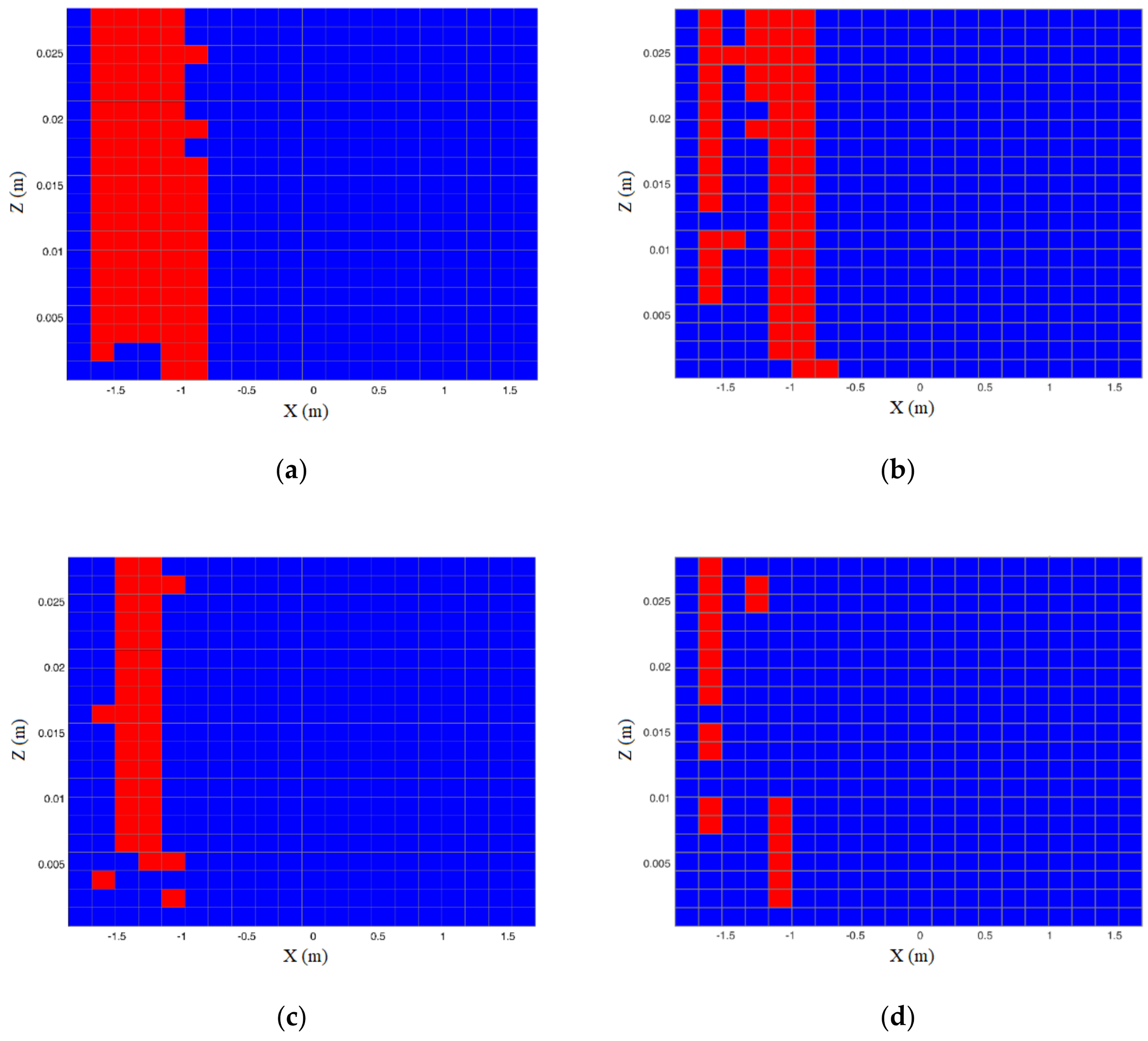[38] showed that particles would not have to remain at the water surface, which is closer to reality. The line-like pattern at the tops of Figure 3a,b also demonstrates the above observation, as the line-like pattern consists of a great number of particles at the water surface. Furthermore, the lag between fluid particles and sediment particles is considered in the diffusivity of Absi et al. [38]. Therefore, the simulation results with the diffusivity of Absi et al. [38] would be made more meaningful than the diffusivity of Rouse [37].

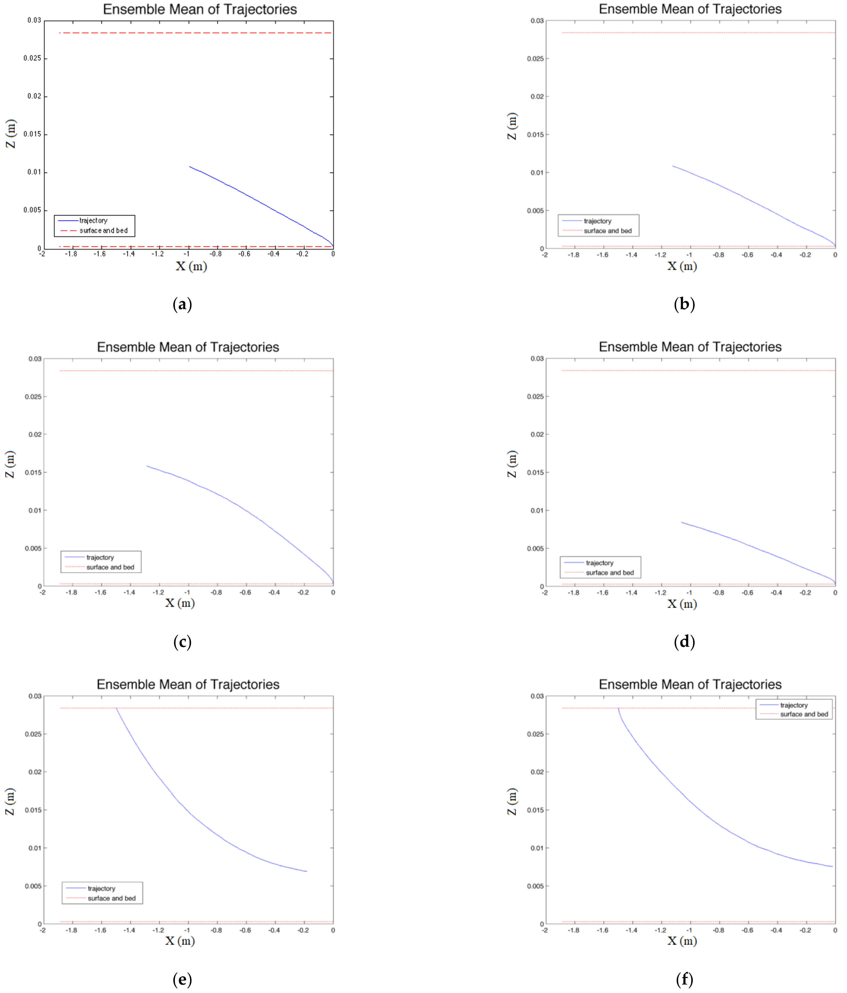
In the aspect of ensemble mean of trajectories (Figure 2), no significant difference between these two diffusivities except for the case of backward tracking with diffusivity of Absi et al. [38]. Figure 2c,d shows that the final position of the mean trajectory by the explicit method is higher than that by the implicit method. It may result from the limitation of implicit methods in which the unknown $Z_n$ cannot be calculated directly. Coupling with the lag between fluid particles and sediment particles considered in the diffusivity, the discrepancies between explicit and implicit methods of diffusivity of Absi et al. [38] consequently might be obvious.

By comparing Figure 1 and Figure 2, one can realize the importance of utilizing a stochastic particle tracking model to assess the variability of particle movement and, subsequently, the likelihood of particle sources.

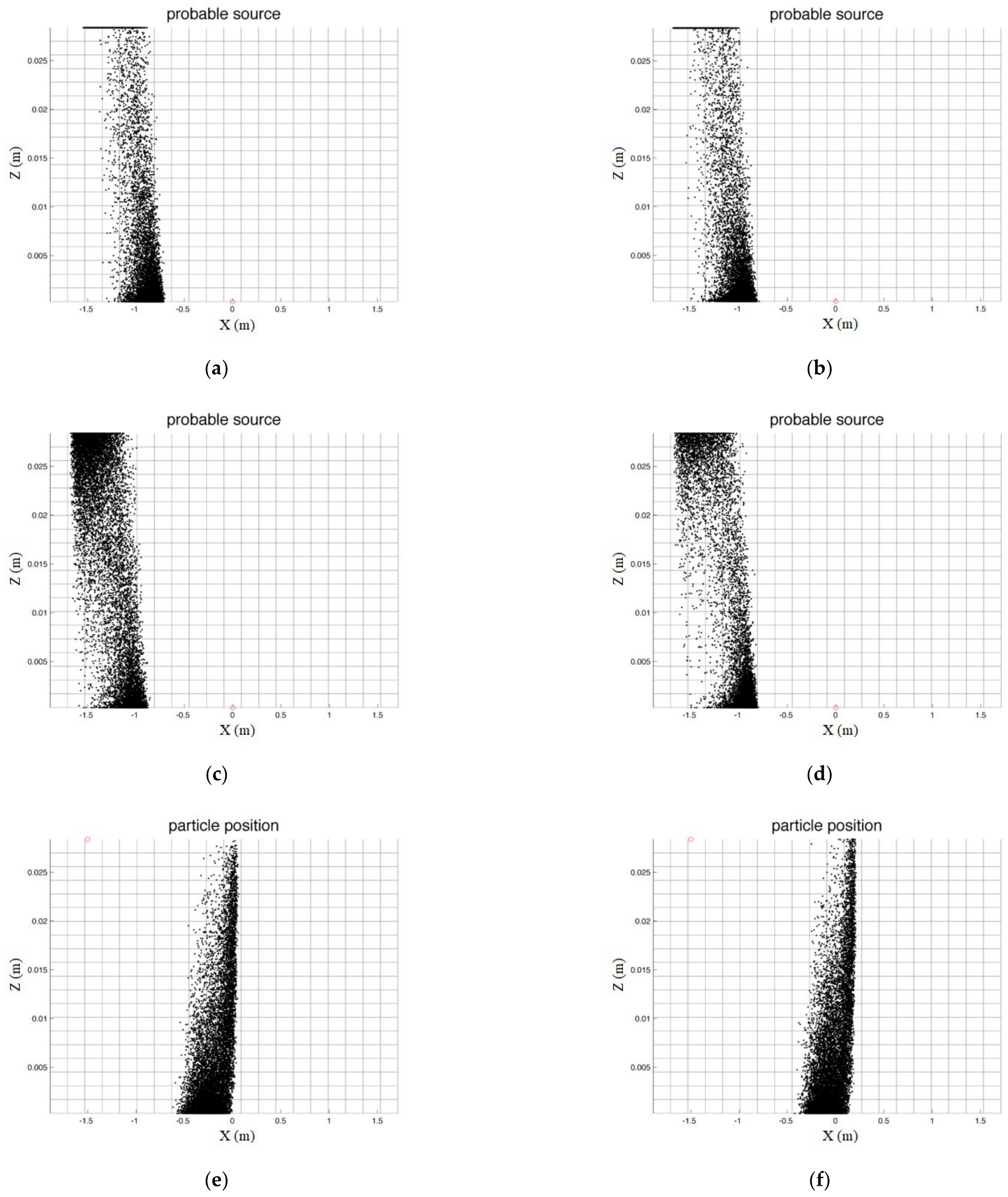
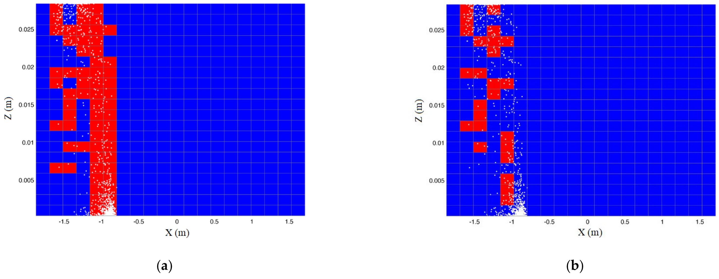
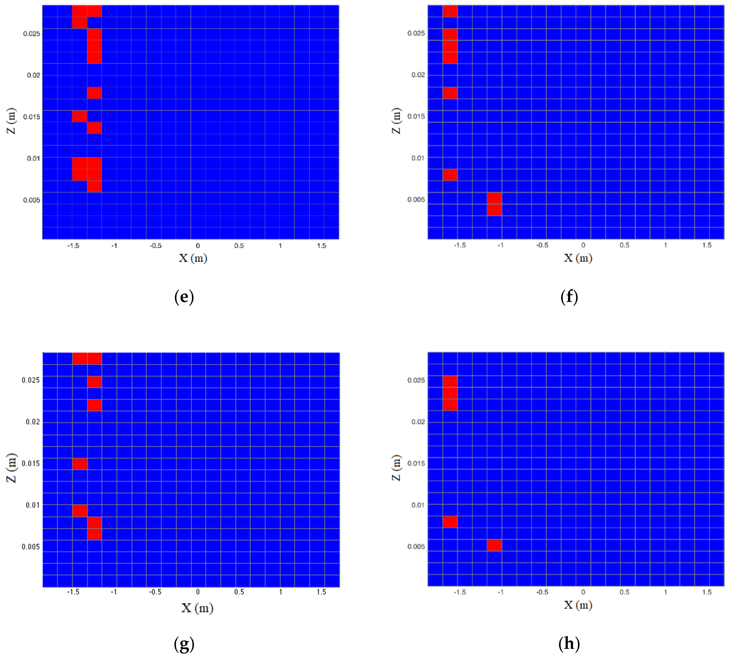
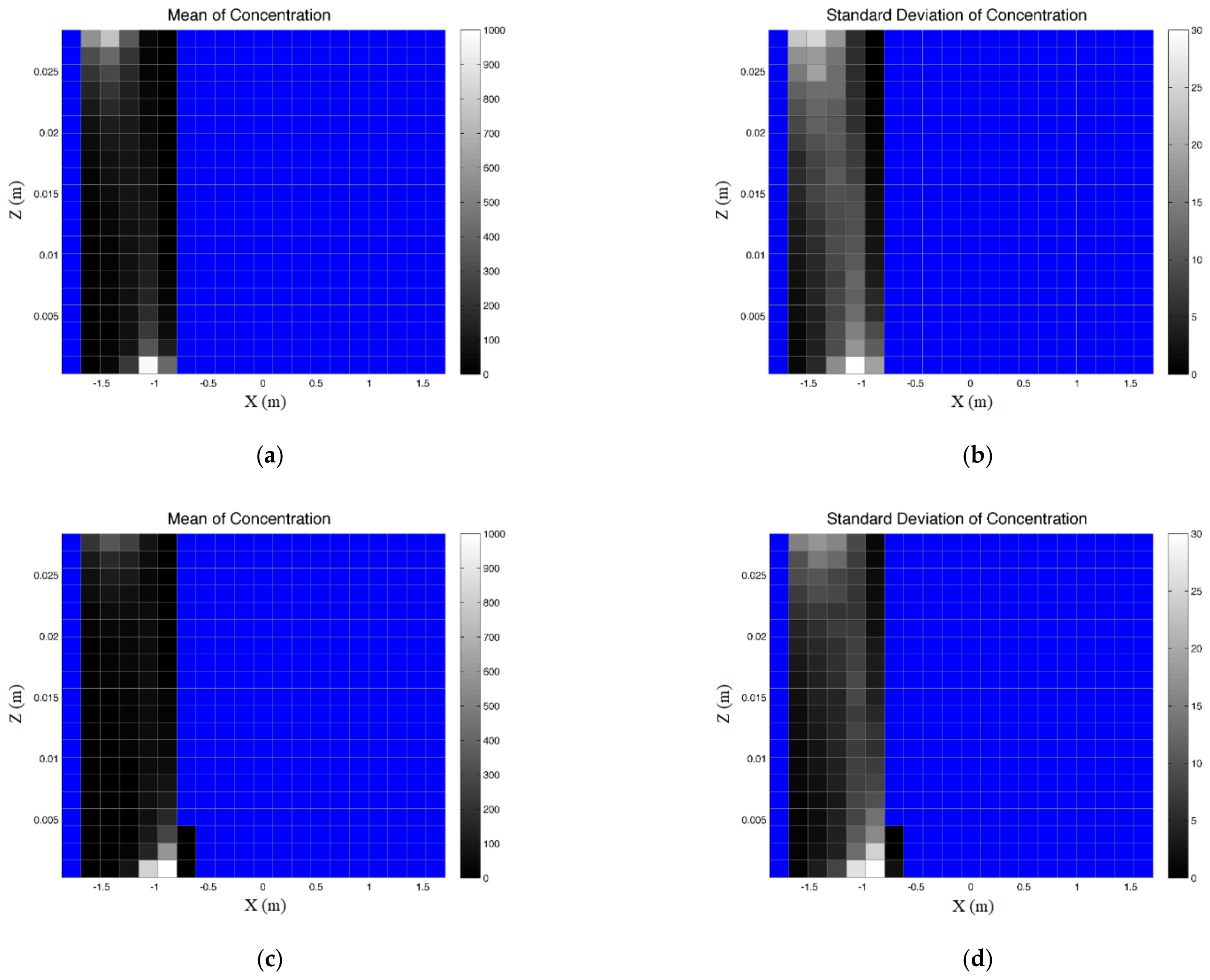
With reference to Figure 3a–d, in all cases of backward tracking with the same initial conditions and parameters, the results reveal that the source is probably at x = −1.5 and z = h. To verify whether particles are deposited on the riverbed at x = 0, two forward tracking tests are carried out to determine the trajectories of particles that are released from the aforementioned point (x = −1.5, z = h). In forward simulations, the assumptions and parameters are the same, but the initial particle positions and tracking directions are different from backward simulations. For forward simulations, the particles are released from the water surface at x = −1.5 m. Two forward tracking cases are modeled by the explicit numerical method (Equations (5) and (6)) with the diffusivity of Rouse [37] or Absi et al. [38].

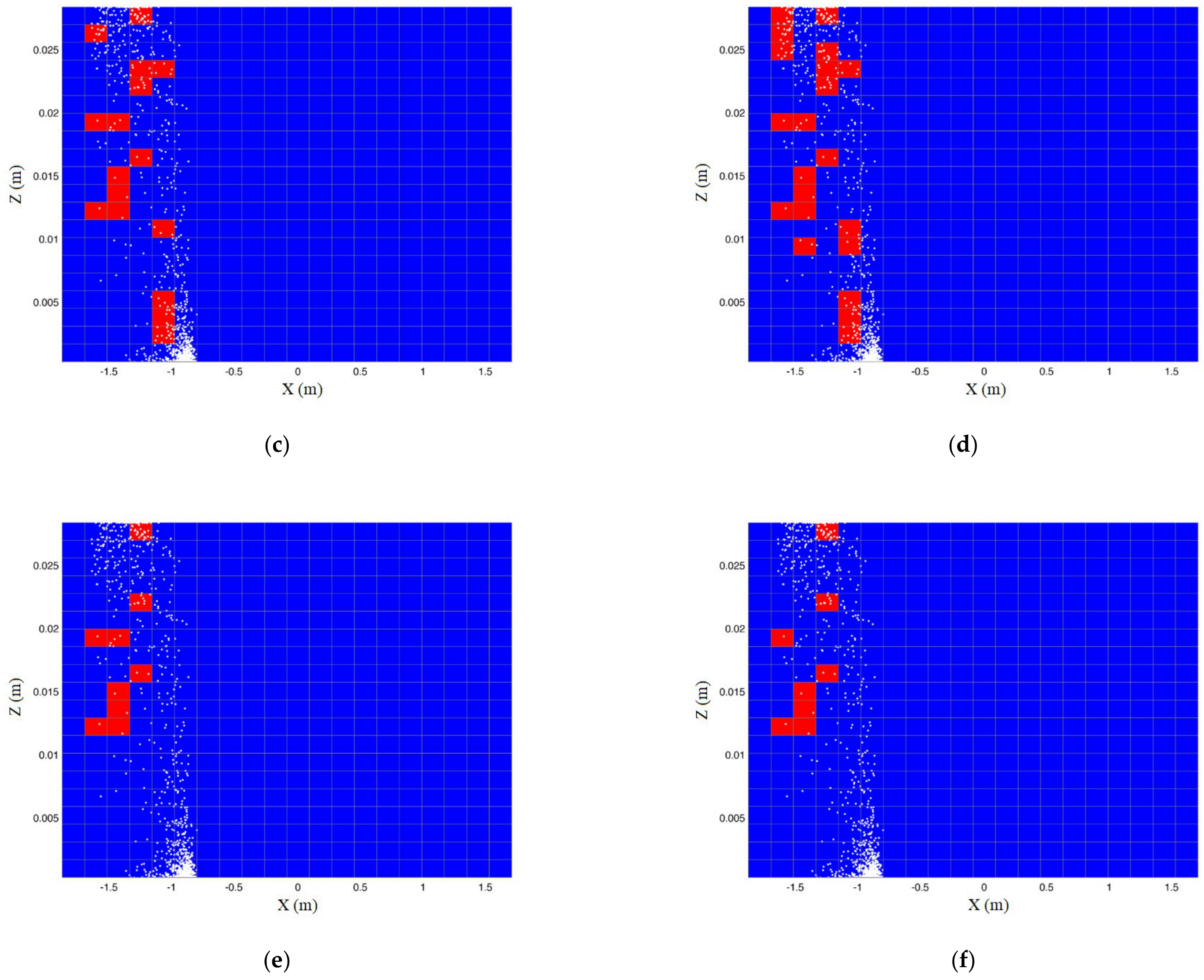
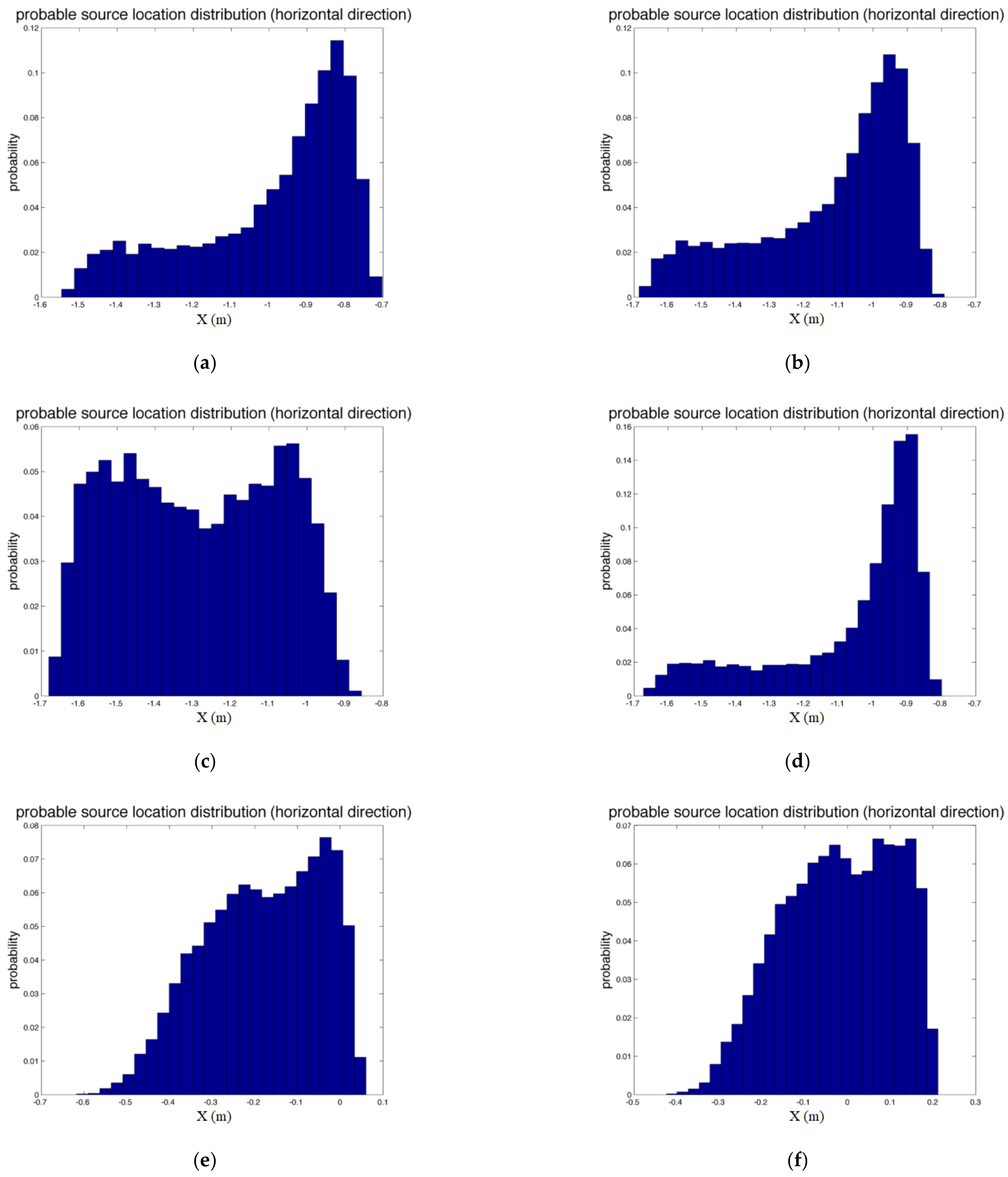
With reference to figures that show particle positions 10 s earlier than the time that sediment particles deposit on the riverbed at x = 0 in the backward tests (Figure 3a,b,d), most of the particles accumulated near the riverbed. Furthermore, with regard to the x-direction, the particles in the near-bed region are closer to the deposition location while those that remain at the surface are farther from that location. This fact may be attributed to the use of the logarithmic velocity distribution, which is larger near the surface, and has the potential to drift particles on the water surface farther. Since the simulation is not run for a long enough time to allow all of the particles to reach the water surface, in more than half of the 10,000 simulations, particles did not arrive at the surface. Therefore, most particles are still close to the riverbed and remain close to the deposited location. Hence, the distribution of final particle locations in the x-direction is skewed toward the origin (Figure 4a,b,d).

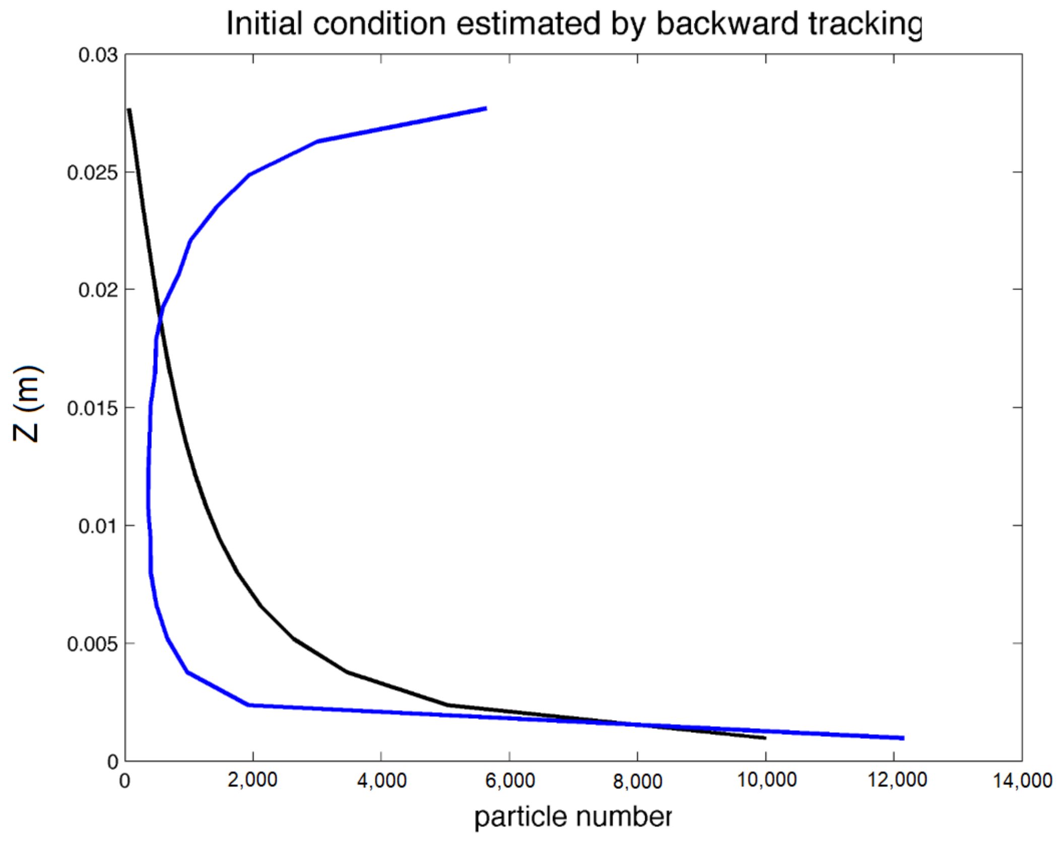
In the z-direction, the probabilities associated with final particle locations decrease sharply as z increases. Notably, the probability associated with the water surface is the second highest owing to the intrinsic characteristic of the governing equation in the z-direction when Rouse’s diffusivity is adopted (Figure 5a,b). However, in tests in which the diffusivity of Absi et al. [38]. is used, the probability that a particle is at the water surface is high and the probability that a particle is in its neighborhood is non-zero (Figure 5c,d). On account of the logarithmically distributed mean drift flow velocity in the horizontal direction, a higher z may be correlated with a greater distance traveled by a particle. As a result, the distribution in the x-direction has two humps because the probability that a particle is near the riverbed or the surface is higher than the probability that it is in any other region. Furthermore, particles are distributed more uniformly in the explicit backward case in which the diffusivity of Absi et al. [38] is used.

The variances of particle positions in both directions increase with time. However, the variance in the x-direction increases continuously with time while that in the z-direction tends to an asymptote. In x-direction, uncertainty is caused by the re-suspension mechanism and sediment concentration gradients in the streamwise direction. Such concentration gradients may cause the shear in the flow to mix particles out which cause the variance to grow in time. If a particle is not re-suspended, then it would stagnate at its location for some time. Therefore, the variability in the stream-wise direction continues to increase. In the vertical direction, the variance initially increases because of the turbulence term. Additionally, it tends to reach an asymptotic constant (or may even decrease if the simulation time is very long) as more particles reach the water surface and their vertical positions cease to change.

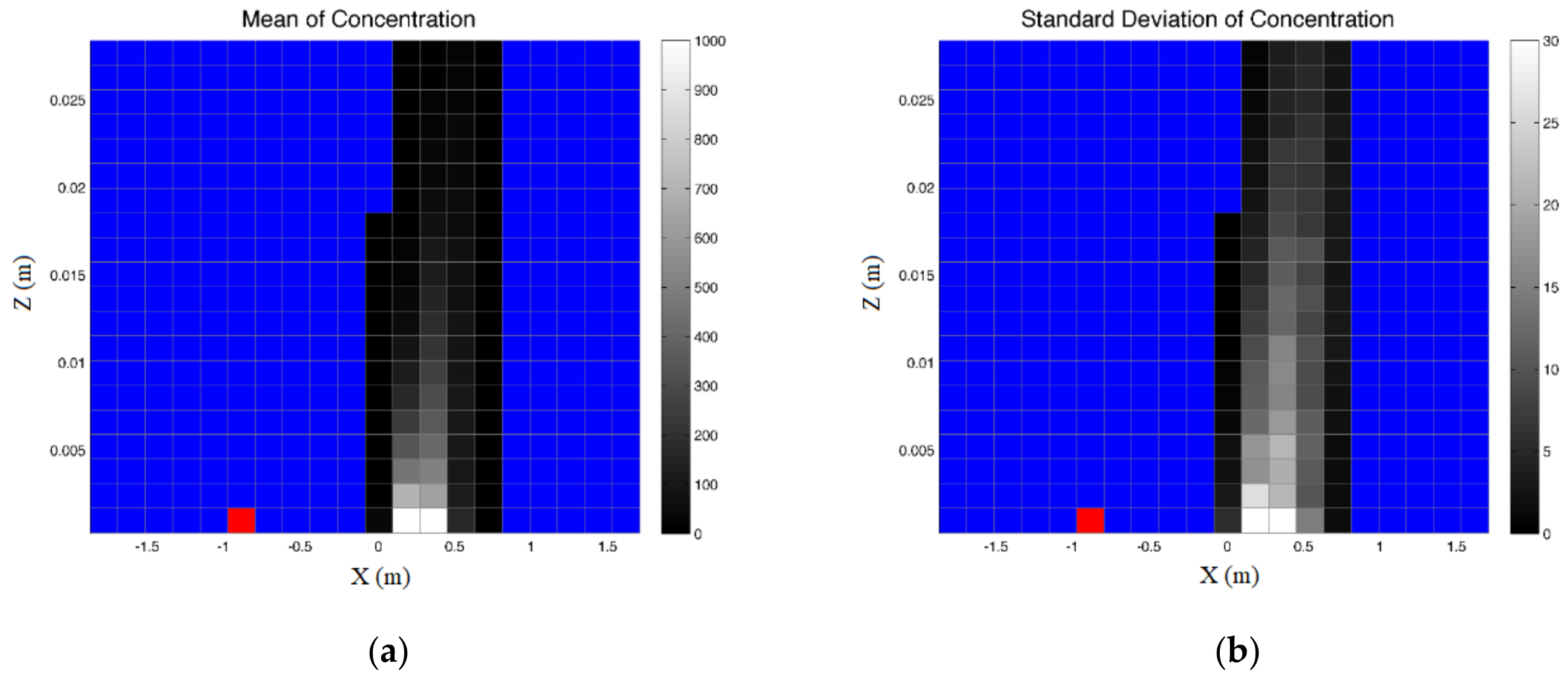
Two forward tests yield insignificantly different results. The overall trajectory is downward in the downstream direction of the channel. According to Figure 5e,f, approximately one-fifth to one-fourth of particles are near the bed. The total number of particles decreases as z increases. Since the overall trend is downward, few particles stay close to the water surface. Two peak values are observed in the distributions in the x-direction at the final time. The left peak is attributable to a large number of particles near the bed, which are transported over short distances. The right peak is attributable to particles that might have arrived from a higher region where flow is fast enough to move particles farther.

4. Development of Backward–Forward Stochastic Particle Tracking Model

The comparison between backward cases and forward cases demonstrates that some probable source regions may be correctly identified. A large proportion of particles are deposited at the deposition point (0, $275\times {10}^{-6}$), indicating that the location (−1.5, 0.0284) might be a probable source. However, no quantitative link or relationship between each source-receptor pair exists. The possibility associated with each probable source that is estimated by backward tracking cannot be quantified even when the forward tracking process is carried out for each of them. Therefore, inspired by Lin et al. [32], the influence function is now introduced to establish or reject each candidate “probable” source that is estimated by backward simulation in this section.

4.1. Influence Function

Uliasz et al. [33] introduced the influence function. In our study, $I\left(x_r,t_r|x,t\right)$ is defined as the influence function of an upstream probable source that is located at $x$ at time t, with respect to a downstream receptor that is located at $x_r$ at time $t_r$.

$$I\left(x_r, t_r|x, t\right)=\frac{1}{N_{tot}}{\displaystyle \sum }_i^{N_{tot}}\delta \left(x_i\left(p\right)-x\right)$$

(22)

$$I_f\left(x_r, t_r|x, t\right)=\frac{n_{sf}}{N_{tot}}$$

(23)

$$I_b\left(x_r, t_r|x, t\right)=\frac{n_{sb}}{N_{tot}}$$

(24)

In Equation (22), $N_{tot}$ is the number of total particles which exist at the source x at time t. Thus, the spatial distribution of concentration at time t should be known, so $N_{tot}$ at each source could be calculated. The delta function $\delta \left(x_i\left(p\right)-x\right)$ represents whether a particle from the upstream source $\left(x, t\right)$ is transported to the downstream receptor $\left(x_r, t_r\right)$. If the $i^{th}$ particle satisfies the above conditions, then the delta function $\delta \left(x_i\left(p\right)-x\right)$ equals one; if it does not, the value of the delta function is zero. Equation (23) can be used to calculate the influence functions of the forward particle tracking process $I_f\left(x_r, t_r|x, t\right)$. The denominator is $N_{tot}$ while the numerator is the number of particles that are transported from a certain source to the receptor during the forward particle tracking process $n_{sf}$.

In the backward particle tracking process, the concept of the influence function $I_b\left(x_r, t_r|x, t\right)$ is physically the same as that in the forward particle tracking process. The total particle number at the source at time $t$ significantly affects the value of the influence function. If the process is reversible, then $I_f\left(x_r, t_r|x, t\right)$ should resemble $I_b\left(x_r, t_r|x, t\right)$. However, in numerical simulations, $I_f\left(x_r, t_r|x, t\right)$ is rarely equivalent to $I_b\left(x_r, t_r|x, t\right)$. A threshold $\epsilon$ is introduced here.

$$\left\{\begin{array}{c}\left|I_f\left(x_r, t_r|x, t\right)-I_b\left(x_r, t_r|x, t\right)\right|<\epsilon , I_f\left(x_r, t_r|x, t\right)\cong I_b\left(x_r, t_r|x, t\right)\\ \left|I_f\left(x_r, t_r|x, t\right)-I_b\left(x_r, t_r|x, t\right)\right|\ge \epsilon , I_f\left(x_r, t_r|x, t\right)\ne I_b\left(x_r, t_r|x, t\right)\end{array}\right.$$

(25)

For a large number of particles, if the difference between $I_f\left(x_r, t_r|x, t\right)$ and $I_b\left(x_r, t_r|x, t\right)$ is smaller than ε, then they are regarded as equal, and the process is regarded as reversible (Equation (25)).

Notably, only the numbers of particles at $\left(x_r, t_r\right)$ and $\left(x, t\right)$ instead of the transport trajectories are considered in the influence function. Namely, although $I_f\left(x_r, t_r|x, t\right)$ is close to $I_b\left(x_r, t_r|x, t\right)$, it is ignored by the influence function whether all the backward trajectories have their corresponding forward trajectories.

The definition of influence function that is used during the simulation process in this study differs slightly from that used in the study of Lin et al. [32]. In the study of Lin et al. [32], the same number of particles (10,000) was released from both the source and the receptor, and the air density gradient was taken into account in modifying the influence function. $N_{tot}$ corresponds to the number of scenarios in the Monte Carlo simulation in their study. However, in this study $N_{tot}$ represents not only the number of scenarios in the Monte Carlo simulations but also the total number of local particles at the sources. The numbers of local particles all exceed 50 and are statistically significant in our Monte Carlo simulations.

4.2. Simulation Process

Figure 8 and Figure 9 present the simulation process.

The details are explained step by step below.

• Establish the domain and divide it into several grid cells. The channel which has the same flow depth as that in Section 3 is divided into 20 layers. Each grid cell is 0.18 m long. In the x-direction, the domain is bounded by (−1.8, 1.8) and so is long enough to observe particle motion within a 10 s simulation if the receptor is at the origin.
• Calculate the number of particles $n_r$ at the deposition point (receptor) as the number of particles in the red rectangle in Figure 9a.
• Use the backward stochastic particle tracking model to trace the receptor grid cell of $n_r$ particles and find the total number of particles that are traced back to each upstream source grid cell ($n_{sb}$), as the total number of hollow blue particles in the blue rectangle in Figure 9a.
• Combine the results in step 3 ($n_{sb}$) with the total number of particles at probable sources ($N_{tot}$) to calculate backward influence functions ($I_b$). In Figure 9b, $N_{tot}$ is the total number of solid and hollow blue particles in the blue rectangle. $N_{tot}$ represents the total number of particles at the source at time t. The hollow particles are traced from the receptor in the backward simulation process.
• Use the results in step 3 with the forward stochastic particle tracking model. Release $N_{tot}$ particles from the middle point of the upstream grid cell to find the number of particles that travel to the receptor $n_{sf}$, as the total number of hollow red particles in the red rectangle in Figure 9c.
• Combine the results in step 5 ($n_{sf}$) with the total number of particles at probable sources $\left(N_{tot}\right)$ to calculate forward influence functions ($I_f$). (Figure 9d)
• Calculate the $n_{sb}$ as well as repeat step 4 to step 6 for each probable source grid identified by the pure backward simulation.
• Map the values of the forward and backward influence functions in the domain at their corresponding source locations.
• Compare and discuss the forward and backward influence functions to evaluate the reversibility and the possibility of probable sources in each grid cell. Determine the threshold value $\epsilon$ and find whether the difference between $I_b$ and $I_f$ is smaller than $\epsilon$.
• Map the most probable source regions.

4.3. A Test of Backward and Forward Influence Functions

In this section, a test of backward and forward influence functions is demonstrated with the same domain as that in Section 4.2. The parameters of the particles, flow conditions and governing equation are same as those in the previous section shown in Table 1. The number of deposited particles at the receptor ($n_r$) is assumed to be 1000. The receptor is at the origin as the initial condition of backward tracking. For each forward tracking process, the initial condition of particle position is at the middle point of the grid of probable sources. The simulation time for both backward and forward tracking is 10 s, which is long enough to observe the trend of the motion of sediments. $N_{tot}$ is relevant to sediment concentration. Thus, the concentration of sediment particles can be introduced below.

The numerical methods applied in this test are implicit backward tracking and explicit forward tracking, all with the diffusivity proposed by Absi et al. [38]. The particle concentrations at time $t_r$ (when particles are transported to and deposited at the receptor) are assumed to follow Rouse’s sediment concentration profile [37]:

$$\frac{C\left(z\right)}{C\left(a\right)}={\left[\left(\frac{h-z}{z}\right)\left(\frac{a}{h-a}\right)\right]}^{w_s/\kappa u_{\ast }}$$

(26)

where $C\left(z\right)$ is the concentration at height $z$; $C\left(a\right)$ is the reference concentration at height $z=a$; $h$ is the flow depth; $w_s$ is the settling velocity; $\kappa$ is the Karman constant, and $u_{\ast }$ is the shear velocity.

In this test, the reference concentration $C\left(a\right)=1000$ is assumed at the bottom layer to represent the number of particles there. The sediment concentration is assumed to be uniform in the stream-wise direction. Therefore, sediment concentration is not a function of x but a function of z. The sediment concentrations within the domain at time $t$ is estimated by backward stochastic particle tracking. Then, the sediment concentrations (total numbers of sediment particles in grid cells, $N_{tot}$, within the domain) at the source are known. In Figure 10, the black dashed line denotes the numbers of particles that are calculated using Rouse’s sediment concentration profile (at time $t_r$), while the blue line denotes the number of particles that are estimated by backward stochastic particle tracking (at time $t$). Both concentrations are independent of x but dependent on z.

To confirm the accuracy of backward tracking, $I_b$ and $I_f$ are compared. Every $I_f$ is regarded as a true value. Then, the relative error of every $I_b$ is calculated and mapped. The relative error is given by the following equation.

$$I_{error}=\frac{\left|I_b-I_f\right|}{I_b}$$

(27)

The difference between $I_f$ and $I_b$ in each grid cell is mapped out. Figure 11 presents the influence functions that are calculated by backward tracking $\left(I_b\right)$ and forward tracking $\left(I_f\right)$. The blue regions are those in which no particle appears ten seconds before time = $t$. The influence function of an upstream grid cell on the receptor (0, $275\times {10}^{-6}$) is shown in a lighter color. The yellow dots in Figure 11c denote the locations of 1000 particles 10 s earlier before they deposited at the receptor. The results are calculated by backward tracking. At $x=-0.9$, the grid cells closer to the riverbed tend to have large $I_b$ and small $I_f$ values. The highest sediment concentrations can be obtained only when locations that are determined by backward simulations are taken into account. However, these grid cells may not be the regions of the most probable sources because of their irreversibility, which is implied by the great difference between the backward and forward influence functions.

To identify the probable source regions, a threshold ε is determined to decide whether the difference between a pair of backward and forward influence functions for a grid cell could be ignored. Figure 12 shows the identified probable source regions with threshold values of 1, 0.8, 0.6, 0.4, 0.2, and 0.1. It can be found that with a lower threshold value, fewer grid cells are probable source regions. Again, the results that are estimated only by backward simulations may not be precise. Nevertheless, the process of backward tracking can assist in scaling down the probable source regions.

5. A Case Study with Explicit and Implicit Backward Tracking Methods

The objective of this case study is to identify the probable source regions of these particles 10 s before the time $t_r$(time $t=t_r-10$) using the backward–forward stochastic particle tracking model. At time $t_r$, sediment particles deposit on the riverbed at x = 0.

5.1. Parameters and Initial Conditions

The diffusivity applied in this case study is that of Absi et al. [38]. Two numerical methods—explicit and implicit—are used during backward simulation while the numerical methods used for forward simulations are always explicit.

In this case study, the domain is the same as the one in Section 4.2. The particle parameters, channel settings, and flow conditions are mostly the same as those in Table 1. The only difference is that the number of deposited particles is 10,000. The concentration is assumed to follow Rouse’s sediment concentration profile as a function of depth with 10,000 particles in the bottom layer at time $t_r$. The sediment concentration is assumed to be uniform in the x-direction. The sediment concentration 10 s before (at time $t$) is estimated using implicit backward simulations. Figure 13 plots the sediment concentrations as functions of z at times $t$ and $t_r$ as blue and black curves, respectively. With the help of this concentration data, $N_{tot}$ as well as the influence function for each probable source candidate can be calculated. $N_{tot}$ in each probable grid is also the number of realizations in Monte Carlo simulations.

5.2. Simulation Results and Discussions

Figure 14, Figure 15 and Figure 16 present the simulation results obtained using explicit and implicit methods. The results obtained using the explicit method are plotted on the left-hand side while those obtained using the implicit method are plotted on the right-hand side.

Figure 14 plots as white dots the 10,000 particle source locations that are estimated from 10,000 backward simulations from the receptor. As discussed in Section 3, the particles tend to cluster near the riverbed and near the water surface.

Figure 15 displays backward influence functions, forward influence functions and the relative error of influence functions. In general, regions with higher backward influence functions seem to appear along with a band from the upper-left to the lower-right. The grid cells with higher backward influence function regions determined using the explicit method significantly differ from those determined using the implicit method.

Two simulations that involve the same processes yield slightly different results because of the stochastic term in the stochastic particle tracking model. This slight difference also suggests that the influence functions and concentrations may not be sufficiently accurate. This is because the concentration distribution obtained based on 10,000 backward simulations only represent a single scenario of the concentration distribution. In regions adjacent to the upstream/downstream area, the forward influence functions may be low, indicating that the influence of this area on the receptor is weak. Accordingly, the backward simulation process roughly identifies the most influential regions, but influence functions are needed to determine probable source regions.

Overall, the relative error in the implicit method is much higher than that in the explicit method, especially in the lower left regions. Therefore, an implicit method may be less accurate in most areas in this case. Notably, the spatial distributions of regions with lower relative errors, corresponding to greater accuracy, differ significantly between the explicit and implicit methods. The left-most section has the least relative error in the backward influence functions. Both the implicit and the explicit methods have a larger error near the riverbed than at the water surface. Furthermore, the regions with higher sediment concentrations computed by only backward simulations do not necessarily imply a higher likelihood of sources. While the explicit method may not identify correctly the probable source regions, the implicit method could assist in identifying such missed probable sources.

After the relative error of the influence functions is calculated, the threshold is set to different values, as depicted in Figure 16. If the threshold is 0.1, the relative error of influence functions is smaller than 10%. The most probable source regions are then identified with a threshold value of 0.1, and their corresponding influence functions are listed in

Table 2. The most probable sources selected out when the threshold is 0.1 and their corresponding influence functions.

No.	$\mathit{x} \left(\mathit{m}\right)$	$\mathit{z} \left(\mathit{m}\right)$	$\mathbf{Backward} \mathbf{Influence} \mathbf{Function} {\mathit{I}}_{\mathit{b}}$	$\mathbf{Backward} \mathbf{Influence} \mathbf{Function} {\mathit{I}}_{\mathit{f}}$
Explicit
47	−1.44	0.0094	0.0427	0.0452
51	−1.44	0.015	0.0932	0.0957
60	−1.44	0.0277	0.1324	0.1229
65	−1.26	0.0066	0.1469	0.1367
66	−1.26	0.008	0.1575	0.1425
76	−1.26	0.0221	0.1153	0.1123
78	−1.26	0.0249	0.0823	0.0782
80	−1.26	0.0277	0.0663	0.0727
Implicit
26	−1.62	0.008	0.0025	0.0025
36	−1.62	0.0221	0.0286	0.0286
37	−1.62	0.0235	0.0296	0.0268
38	−1.62	0.0249	0.0386	0.035
84	−1.08	0.0052	0.1182	0.1197

.

In general, the sources that are identified by the explicit method tend to have a higher influence function, so the explicit method identifies locations that have a stronger higher influence on the receptor. However, the implicit method performs poorly in identifying locations with higher influence functions.

6. Discussion about Probable Sources Based on Ensemble Mean and Ensemble Standard Deviation of Spatial Sediment Concentration Distribution

Oh et al. [28] suggested that sediment concentration can be estimated by the spatial distribution of particles using the stochastic particle tracking model. As displayed in Section 3, one numerical experiment that involved 10,000 simulations can provide the ensemble mean and the ensemble variance of particle locations. However, as depicted in Figure 14, the same initial conditions can lead to different spatial concentration distributions.

Hence, the numerical experiment that involved 10,000-round Monte Carlo simulations to determine one unique spatial concentration distribution is repeated 100 times. Then, 100 scenarios of spatial concentration distributions can be obtained. In this section, the ensemble mean and the ensemble standard deviation of spatial concentration distributions in backward tracking are computed. The position of the receptor is also located at the origin. Since the probable regions that are identified in Section 5 are of great interest, 100 spatial concentration distributions are also computed by forward tracking from these probable source regions. The ensemble statistics of the spatial concentration distributions and the influence of these sources to the receptor can thus be discussed.

6.1. Parameters and Initial Conditions

Table 3. Particle, flow conditions and simulation parameters.

Parameter	Unit	Value
Diameter ($D$)	$\mathrm{m}$	$275\times {10}^{-6}$
Density (${\rho }_s$)	$\mathrm{k}\mathrm{g}/{\mathrm{m}}^3$	$1050$
Lift coefficient ($C_L$)		$0.21$
Shear velocity ($u_{\ast }$)	$\mathrm{m}/\mathrm{s}$	$0.0086$
Settling velocity ($w_s$)	$\mathrm{m}/\mathrm{s}$	$0.0025$
Reference height ($z_b$)	$\mathrm{m}$	$275\times {10}^{-6}$
Roughness height ($ks$)	$\mathrm{m}$	$275\times {10}^{-6}$
Flow depth (h)	$\mathrm{m}$	0.0284
Mean drift flow velocity $(\overline{u}$)	$\mathrm{m}/\mathrm{s}$	0.143
Mean drift flow velocity $(\overline{w}$)	$\mathrm{m}/\mathrm{s}$	0
Time step ($dt$)	$\mathrm{s}$	0.01
Simulation Time ($T$)	$\mathrm{s}$	10

presents the parameters of particles, flow conditions, simulation time and the time step. In the backward simulation, 10,000 particles are traced backward for 10 s from the receptor $\left(0, 275\times {10}^{-6}\right)$ for each realization of spatial sediment concentration distributions. With respect to forward simulations, 10,000 particles are traced forward for 10 s from each probable source location identified in Section 5 for each realization of the spatial sediment concentration distributions. A total of 100 realizations of spatial concentration distributions are computed to estimate the ensemble means and ensemble standard deviations. As Figure 16 indicates, when the threshold value is 0.1, eight grid cells and five grid cells are suggested to be the probable source regions in explicit and implicit backward methods, respectively.

6.2. Simulation Results and Discussion

6.2.1. Backward Simulation

Figure 17 presents the ensemble mean and ensemble standard deviation of spatial sediment concentration distributions that are estimated using explicit and implicit methods. Most of the particles are traced back to the riverbed at about $x=-1$. With respect to the ensemble means, the highest concentration obtained by the explicit method is farther from the receptor than that obtained by the implicit method. Another region of high concentration appears on the water surface at about $x=-1.5$. The particles tend to be distributed more uniformly in the explicit method. The highest ensemble means of concentration that are obtained by the explicit method and implicit method are 975.93 and 4017.1 particles per grid cell, respectively. The difference is considerable, implying that at least one of these two values are far from the true value.

The maximum of the ensemble standard deviations obtained by the explicit and implicit methods, are 30.36 and 26.60, respectively. The difference of the ensemble standard deviations in the grid cell with the highest concentration between the two numerical methods is quite low. However, compared to the ensemble mean value, the ensemble standard deviation in the grid cell with the highest concentration is relatively high in the explicit method.

As depicted in Figure 17, ensemble standard deviations tend to be higher where ensemble means are higher, according to both the explicit method and the implicit method. This result is consistent with those obtained by Oh et al. [28]. This highest standard deviation may be a significant cause of why only the grid cell with the highest concentration, estimated only by the backward simulation, may not necessarily be the most probable source. However, another reason why the area of highest concentration is not the region of the most probable source may be attributed to the large difference between the estimated ensemble mean of the sediment concentration and the true value.

6.2.2. Forward Simulation with Explicit Method

Table 4. The ensemble mean and ensemble standard deviation of spatial sediment concentration distribution from 8 different probable sources.

Probable Sources	Ensemble Mean	Ensemble Standard Deviation
Particles are released from (−1.44, 0.0094)
Particles are released from (−1.44, 0.015)
Particles are released from (−1.44, 0.0277)
Particles are released from (−1.26, 0.0066)
Particles are released from (−1.26, 0.008)
Particles are released from (−1.26, 0.0221)
Particles are released from (−1.26, 0.0249)
Particles are released from (−1.26, 0.0277)

displays the ensemble mean and ensemble standard deviation of the spatial sediment concentration distribution from eight probable sources as determined using the explicit method in Section 5. The blue color indicates an absence of particles. A lighter color represents a higher ensemble mean or ensemble standard deviation. The red grid cell represents the location of a probable source from which particles are released. For these aforementioned simulations the spatial sediment distributions cover the receptor grid cell in all simulations, demonstrating the superior performance of the explicit method.

Table 5. The ensemble mean and ensemble and ensemble standard deviation of concentration at the receptor grid (explicit method).

Simulation No.	Ensemble Mean of Concentration at the Receptor (Bead)	Ensemble Standard Deviation of Concentration at the Receptor (Bead)
Ex-1	510.59	21.6334
Ex-2	797.4	26.9035
Ex-3	1239.7	34.1854
Ex-4	1370.6	29.7602
Ex-5	1404.4	32.6969
Ex-6	968	30.9169
Ex-7	799.2	24.5801
Ex-8	691	27.7581

presents the ensemble mean and ensemble standard deviation of concentrations (represented as the number of particles) in the receptor grid cell. In all simulations, the concentration of the particles at the receptor exceeds 500 particles per grid. Namely, the probability that a particle is transported to the receptor from these sources exceeds 5%. This probability is relatively high, as the sediment is present over a large area. Moreover, the grid cells with the first or second highest concentration are receptor grid cells in most of the simulations. However, a grid cell with a higher ensemble mean concentration normally also has a higher ensemble standard deviation (variability) in forward simulations.

6.2.3. Forward Simulation with Implicit Method

Table 6. Ensemble mean and ensemble standard deviation of the spatial sediment concentration distribution.

Probable Sources	Ensemble Mean	Ensemble Standard Deviation
Particles are released from (−1.62, 0.008)
Particles are released from (−1.62, 0.0221)
Particles are released from (−1.62, 0.0235)
Particles are released from (−1.62, 0.0249)
Particles are released from (−1.08, 0.0052)

presents the ensemble mean and ensemble standard deviation of the spatial sediment concentrations when particles are traced forward from the probable sources that are identified by the implicit method. The notation and representation of the results are similar to those in the explicit method. As the table shows, the receptor was covered by the sediment in all five simulations. However, in most of these simulations, the ensemble mean of the concentrations at the receptor was lower than that obtained using the explicit method.

For simulations Im-2, Im-3 and Im-4, the concentration is around 200 to 300 particles per grid cell (about 2–3%); for simulation Im-1, the ensemble mean concentration is only 29.3 particles per grid cell (0.293%) (

Table 7. The ensemble mean and standard deviation of concentration at the receptor grid (explicit method).

Simulation No.	Ensemble Mean	Ensemble Standard Deviation
Im-1	29.3	5.0887
Im-2	243.33	16.8169
Im-3	272.79	19.1466
Im-4	303.42	17.8372
Im-5	1033.8	29.4296

). Only the ensemble mean of the concentration in simulation Im-5 is as high as that obtained using the explicit method. Therefore, the implicit method underperforms the explicit method in determining sources with a strong influence on the receptor. Again, a higher ensemble mean of concentration corresponds to a higher ensemble standard deviation in these simulations. None of the simulation cases is an exception to this rule.

6.2.4. Forward Simulation from Non-Probable Source

A grid cell at (−0.9, 0) is a high concentration, as estimated by either the backward explicit method or implicit method. In Section 5, neither the explicit nor the implicit method suggests this region as a probable source. Now, the ensemble mean and the ensemble standard deviation of the concentrations are computed after the particles have traveled for 10 s (Figure 18).

Although the receptor grid is covered by the particles, the concentration of sediment is low in the receptor grid cell. Only 31.77 of 10,000 particles are transported to the receptor from this region. The results again demonstrate that the highest concentration, estimated by the backward simulation alone, suffices to identify the probable source. Furthermore, the probability of particle transporting to the receptor from a non-probable source is much lower than that from probable sources, no matter which numerical methods is adopted.

7. Conclusions and Recommendations

Source identification is useful for containment prevention or ecological conservation. It also supports our understanding of particle behaviors, which can aid in efficiently tackling sedimentation problems. However, there is limited research applying the backward–forward particle tracking model to identify sedimentation sources. In this work, a state-of-the-art Lagrangian stochastic particle tracking model is applied to identify sedimentation sources. The diffusivities proposed by Rouse [37] and Absi et al. [38] are both considered. It is found that not only the non-zero value of the diffusivity is performed at the water surface, but the lag between fluid and sediment particles can be considered by the diffusivity of Absi et al. [38].

Inspired by Lin et al. [32], a backward–forward stochastic particle tracking model is formed with the help of influence functions. The sediment concentrations in upstream regions must be known a priori to determine the influence functions. A case study of source identification using the stochastic particle tracking model is presented. In this backward–forward SD-PTM, the outcome from the backward simulation can be used as a reference in limiting the regions of probable sources. With respect to the numerical method, the explicit method performs better in identifying sources with higher influence functions than the implicit method does. In the forward simulations, the implicit method may underperform the explicit method when determining probable sources. Moreover, the probabilities are much higher comparing to simulations from non-probable sources (only about 0.3%) no matter which numerical method is applied.

The area of high concentrations also has a high standard deviation in concentrations. The results of probable source regions only identified by backward simulations may not be indicative, but they scale down the probable source regions. Both the forward and the backward influence function can be improved when calculated using the ensemble mean of particle concentrations. However, the computation time would be very large if all of the concentrations are ensemble means. In addition, the trajectories are not presented as outcomes of the backward–forward SD-PTM and inputs of influence functions. Whether there exist corresponding trajectories in pure backward and forward simulations is considered in deciding influence functions, then the backward–forward SD-PTM could be made more convincing. For example, particle trajectories could be simplified, and the similarity between patterns in the forward and backward simulations could be considered.

Finally, the computational time for backward-forward particle tracking in this preliminary study remains considerable. To solve a large spatial-temporal scale real-world engineering problem such as reservoir sedimentation, the computational demand may be met by more efficient numerical approaches and advanced computing technology.

References

1. U.S. Department of the Interior Bureau of Reclamation. Hydrology, Hydraulics, and Sediment Studies for the Matilija Dam Ecosystem Restoration Project. 2006. 323p. Available online: https://calisphere.org/item/ark:/86086/n2nz879g/ (accessed on 29 April 2021).
2. California State Coastal Conservancy. Staff Recommendation, May 24, 2007: San Clemente Dam Removal Project Technical Assistance. 2007. Available online: https://calisphere.org/item/ark:/86086/n2p84bk6/ (accessed on 29 April 2021).
3. Wang, H.-W.; Kondolf, G.M. Upstream Sediment-Control Dams: Five Decades of Experience in the Rapidly Eroding Dahan River Basin, Taiwan. JAWRA J. Am. Water Resour. Assoc. 2014, 50, 735–747. [Google Scholar] [CrossRef]
4. Kondolf, G.M.; Gao, Y.; Annandale, G.W.; Morris, G.L.; Jiang, E.; Zhang, J.; Cao, Y.; Carling, P.; Fu, K.; Guo, Q.; et al. Sustainable sediment management in reservoirs and regulated rivers: Experiences from five continents. Earth’s Future 2014, 2, 256–280. [Google Scholar] [CrossRef]
5. McCully, P. Silenced Rivers: The Ecology and Politics of Large Dams; Zed Books: London, UK, 1996. [Google Scholar]
6. Shang, P.; Na, X.; Kamae, S. Chaotic analysis of time series in the sediment transport phenomenon. Chaossolitons Fractals 2009, 41, 368–379. [Google Scholar] [CrossRef]
7. Taiwan Water Resources Agency. The Operating Report of Reservoirs in Taiwan in 2012. 2012. Available online: http://wuss.wra.gov.tw/annuals.aspx (accessed on 29 April 2021). (In Chinese)
8. Lee, H.-Y.; Lin, Y.-T.; Chiu, Y.-J. Quantitative Estimation of Reservoir Sedimentation from Three Typhoon Events. J. Hydrol. Eng. 2006, 11, 362–370. [Google Scholar] [CrossRef]
9. Keshavarzi, A.; Gheisi, A. Three-dimensional fractal scaling of bursting events and their transition probability near the bed of vortex chamber. Chaos Solitons Fractals 2007, 33, 342–357. [Google Scholar] [CrossRef]
10. Keramaris, E. Turbulent structure in uniform inclined open channel flow over different rough porous beds. Int. J. Sediment Res. 2017, 32, 45–52. [Google Scholar] [CrossRef]
11. Shiono, K.; Knight, D.W. Turbulent open-channel flows with variable depth across the channel. JFM 1991, 222, 617–646. [Google Scholar] [CrossRef]
12. Yen, B.C. Open Channel Flow Resistance. J. Hydraul. Eng. 2002, 128, 20–39. [Google Scholar] [CrossRef]
13. Van Rijn, L.C. Principles of Sediment Transport in Rivers, Estuaries and Coastal Seas; Aqua Publications: London, UK, 1993; Volume 1006. [Google Scholar]
14. Ziaei, A.N.; Keshavarzi, A.R.; Homayoun, E. Fractal scaling and simulation of velocity components and turbulent shear stress in open channel flow. Chaossolitons Fractals 2005, 24, 1031–1045. [Google Scholar] [CrossRef]
15. Tsai, C.W.; Huang, S.H. Modeling suspended sediment transport under influence of turbulence ejection and sweep events. Water Resour. Res. 2019, 55, 5379–5393. [Google Scholar] [CrossRef]
16. Kuai, K.Z.; Tsai, C.W. Discrete-time Markov chain model for transport of mixed-size sediment particles under unsteady flow conditions. J. Hydrol. Eng. 2016, 21, 04016039. [Google Scholar] [CrossRef]
17. Tsai, C.W.; Hung, S.Y.; Wu, T.-H. Stochastic sediment transport: Anomalous diffusions and random movement. Stoch. Environ. Res. Risk Assess. 2020, 34, 397–413. [Google Scholar] [CrossRef]
18. Batchelder, H.P. Forward-in-Time-/Backward-in-Time-Trajectory (FITT/BITT) Modeling of Particles and Organisms in the Coastal Ocean. J. Atmos. Ocean. Technol. 2006, 23, 727–741. [Google Scholar] [CrossRef]
19. Isobe, A.; Kako, S.i.; Chang, P.-H.; Matsuno, T. Two-Way Particle-Tracking Model for Specifying Sources of Drifting Objects: Application to the East China Sea Shelf. J. Atmos. Ocean. Technol. 2009, 26, 1672–1682. [Google Scholar] [CrossRef]
20. Heemink, A. Stochastic modelling of dispersion in shallow water. Stoch. Hydrol. Hydraul. 1990, 4, 161–174. [Google Scholar] [CrossRef] [Green Version]
21. Hunter, J.; Craig, P.; Phillips, H. On the use of random walk models with spatially variable diffusivity. J. Comput. Phys. 1993, 106, 366–376. [Google Scholar] [CrossRef]
22. Harris, A.R.; Davidson, C.I. A Monte Carlo model for soil particle resuspension including saltation and turbulent fluctuations. Aerosol Sci. Technol. 2009, 43, 161–173. [Google Scholar] [CrossRef]
23. Ancey, C. Stochastic modeling in sediment dynamics: Exner equation for planar bed incipient bed load transport conditions. J. Geophys. Res. Earth Surf. 2010, 115. [Google Scholar] [CrossRef]
24. Tsai, C.W.; Lin, E.Y.; Hung, S.Y. Incorporating a trend analysis of large flow perturbations into stochastic modeling of particle transport in open channel flow. J. Hydrol. 2016, 541, 689–702. [Google Scholar] [CrossRef] [Green Version]
25. Man, C.; Tsai, C.W. Stochastic Partial Differential Equation-Based Model for Suspended Sediment Transport in Surface Water Flows. J. Eng. Mech. 2007, 133, 422–430. [Google Scholar] [CrossRef]
26. Oh, J.; Tsai, C.W. A stochastic jump diffusion particle-tracking model (SJD-PTM) for sediment transport in open channel flows. Water Resour. Res. 2010, 46. [Google Scholar] [CrossRef]
27. Tsai, C.W.; Man, C.; Oh, J. Stochastic particle based models for suspended particle movement in surface flows. Int. J. Sediment Res. 2014, 29, 195–207. [Google Scholar] [CrossRef]
28. Oh, J.; Tsai, C.W.; Choi, S.-U. Quantifying the Uncertainty Associated with Estimating Sediment Concentrations in Open Channel Flows Using the Stochastic Particle Tracking Method. J. Hydraul. Eng. 2015, 141, 04015031. [Google Scholar] [CrossRef]
29. Tsai, C.W.; Hung, S.Y.; Oh, J. A stochastic framework for modeling random-sized batch arrivals of sediment particles into open channel flows. Stoch. Environ. Res. Risk Assess. 2018, 32, 1939–1954. [Google Scholar] [CrossRef]
30. Oh, J.; Choi, J.-I.; Choi, S.-U.; Tsai, C.W. Physically Based Probabilistic Analysis of Sediment Deposition in Open Channel Flow. J. Hydraul. Eng. 2017, 143, 04016106. [Google Scholar] [CrossRef]
31. Spivakovskaya, D.; Heemink, A.W.; Milstein, G.N.; Schoenmakers, J.G.M. Simulation of the transport of particles in coastal waters using forward and reverse time diffusion. Adv. Water Resour. 2005, 28, 927–938. [Google Scholar] [CrossRef]
32. Lin, J.C.; Gerbig, C.; Wofsy, S.C.; Andrews, A.E.; Daube, B.C.; Davis, K.J.; Grainger, C.A. A near-field tool for simulating the upstream influence of atmospheric observations: The Stochastic Time-Inverted Lagrangian Transport (STILT) model. J. Geophys. Res. Atmos. 2003, 108. [Google Scholar] [CrossRef] [Green Version]
33. Uliasz, M.; Pielke, R.A. Receptor-oriented Lagrangian-Eulerian model of mesoscale air pollution dispersion. Comput. Tech. Environ. Stud. 1990, 57–68. [Google Scholar]
34. Seibert, P.; Frank, A. Source-receptor matrix calculation with a Lagrangian particle dispersion model in backward mode. Atmos. Chem. Phys. 2004, 4, 51–63. [Google Scholar] [CrossRef] [Green Version]
35. Kaftori, D.; Hetsroni, G.; Banerjee, S. Particle behavior in the turbulent boundary layer. I. Motion, deposition, and entrainment. Phys. Fluids 1995, 7, 1095–1106. [Google Scholar] [CrossRef]
36. Wu, F.-C.; Lin, Y.-C. Pickup Probability of Sediment under Log-Normal Velocity Distribution. J. Hydraul. Eng. 2002, 128, 438–442. [Google Scholar] [CrossRef] [Green Version]
37. Rouse, H. Modern conceptions of the mechanics of turbulence. Trans. Am. Soc. Civ. Eng. 1937, 102, 463–543. [Google Scholar] [CrossRef]
38. Absi, R.; Marchandon, S.; Lavarde, M. Turbulent Diffusion of Suspended Particles: Analysis of the Turbulent Schmidt Number. Defect Diffus. Forum 2011, 312–315, 794–799. [Google Scholar] [CrossRef]
39. Visser, A.W. Using random walk models to simulate the vertical distribution of particles in a turbulent water column. Mar. Ecol. Prog. Ser. 1997, 158, 275–281. [Google Scholar] [CrossRef] [Green Version]
40. Ross, O.N.; Sharples, J. Recipe for 1-D Lagrangian particle tracking models in space-varying diffusivity. Limnol. Oceanogr. Methods 2004, 2, 289–302. [Google Scholar] [CrossRef] [Green Version]
Figure 1. Sample paths randomly selected from 10,000 simulations: (a) sample paths of backward tracking tests with the diffusivity of Rouse [37], using the explicit method; (b) sample paths of backward tracking tests with the diffusivity of Rouse [37], using the implicit method; (c) sample paths of backward tracking tests with the diffusivity of Absi et al. [38], using the explicit method; (d) sample paths of backward tracking tests with the diffusivity of Absi et al. [38], using the implicit method; (e) sample paths of forward tracking tests with the diffusivity of Rouse [37], using the explicit method; (f) sample paths of forward tracking tests with the diffusivity of Absi et al. [38], using the explicit method.
Mathematics 09 01263 g001
Figure 2. Mean Trajectory: (a) mean trajectory of backward tracking tests with the diffusivity of Rouse [37], using the explicit method; (b) mean trajectory of backward tracking tests with the diffusivity of Rouse [37], using the implicit method; (c) mean trajectory of backward tracking tests with the diffusivity of Absi et al. [38], using the explicit method; (d) mean trajectory of backward tracking tests with the diffusivity of Absi et al. [38], using the implicit method; (e) mean trajectory of forward tracking tests with the diffusivity of Rouse [37], using the explicit method; (f) mean trajectory of forward tracking tests with the diffusivity of Absi et al. [38], using the explicit method.
Mathematics 09 01263 g002
Figure 3. Final particle positions of 10,000 simulations: (a) positions of probable sources in backward tracking tests with the diffusivity of Rouse [37], using the explicit method; (b) positions of probable sources in backward tracking tests with the diffusivity of Rouse [37], using the implicit method; (c) positions of probable sources in backward tracking tests with the diffusivity of Absi et al. [38], using the explicit method; (d) positions of probable sources in backward tracking tests with the diffusivity of Absi et al. [38], using the implicit method; (e) final particle positions in forward tracking tests with the diffusivity of Rouse [37], using the explicit method; (f) final particle positions in forward tracking tests with the diffusivity of Absi et al. [38], using the explicit method.
Mathematics 09 01263 g003
Figure 4. Final probable particle location distribution in the x-direction: (a) final probable source location distribution in backward tracking tests with the diffusivity of Rouse [37], using the explicit method; (b) final probable source location distribution in backward tracking tests with the diffusivity of Rouse [37], using the implicit method; (c) final probable source location distribution in backward tracking tests with the diffusivity of Absi et al. [38], using the explicit method; (d) final probable source location distribution in backward tracking tests with the diffusivity of Absi et al. [38], using the implicit method; (e) final particle location distribution in forward tracking tests with the diffusivity of Rouse [37], using the explicit method; (f) final particle location distribution in forward tracking tests with the diffusivity of Absi et al. [38], using the explicit method.
Mathematics 09 01263 g004
Figure 5. Final probable particle location distribution in the z-direction: (a) final probable source location distribution in backward tracking tests with the diffusivity of Rouse [37], using the explicit method; (b) final probable source location distribution in backward tracking tests with the diffusivity of Rouse [37], using the implicit method; (c) final probable source location distribution in backward tracking tests with the diffusivity of Absi et al. [38], using the explicit method; (d) final probable source location distribution in backward tracking tests with the diffusivity of Absi et al. [38], using the implicit method; (e) final particle location distribution in forward tracking tests with the diffusivity of Rouse [37], using the explicit method; (f) final particle location distribution in forward tracking tests with the diffusivity of Absi et al. [38], using the explicit method.
Mathematics 09 01263 g005
Figure 6. Final particle location variance in the x-direction: (a) final probable source location variance in backward tracking tests with the diffusivity of Rouse [37], using the explicit method; (b) final probable source location variance in backward tracking tests with the diffusivity of Rouse [37], using the implicit method; (c) final probable source location variance in backward tracking tests with the diffusivity of Absi et al. [38], using the explicit method; (d) final probable source location variance in backward tracking tests with the diffusivity of Absi et al. [38], using the implicit method; (e) final particle location variance in forward tracking tests with the diffusivity of Rouse [37], using the explicit method; (f) final particle location variance in forward tracking tests with the diffusivity of Absi et al. [38], using the explicit method.
Mathematics 09 01263 g006
Figure 7. Final particle location variance in the z-direction: (a) final probable source location variance in backward tracking tests with the diffusivity of Rouse [37], using the explicit method; (b) final probable source location variance in backward tracking tests with the diffusivity of Rouse [37], using the implicit method; (c) final probable source location variance in backward tracking tests with the diffusivity of Absi et al. [38], using the explicit method; (d) final probable source location variance in backward tracking tests with the diffusivity of Absi et al. [38], using the implicit method; (e) final particle location variance in forward tracking tests with the diffusivity of Rouse [37], using the explicit method; (f) final particle location variance in forward tracking tests with the diffusivity of Absi et al. [38], using the explicit method.
Mathematics 09 01263 g007
Figure 8. Simulation process of backward–forward stochastic particle tracking model.
Mathematics 09 01263 g008
Figure 9. The procedure of the backward–forward stochastic particle tracking model: (a) tracing back particles in the receptor grid cell; (b) calculating the backward influence function; (c) releasing and tracing the particles from the upstream source cell; (d) calculating the forward influence function.
Mathematics 09 01263 g009
Figure 10. Sediment concentrations before and after backward PTM based on Rouse’s formula, represented as particle numbers.
Mathematics 09 01263 g010
Figure 11. (a) Backward influence functions; (b) forward influence functions; (c) the relative error between backward and forward influence functions.
Mathematics 09 01263 g011aMathematics 09 01263 g011b
Figure 12. Probable source regions with different threshold values; (a) threshold value is 1; (b) threshold value is 0.8; (c) threshold value is 0.6; (d) threshold value is 0.4; (e) threshold value is 0.2; (f) threshold value is 0.1.
Mathematics 09 01263 g012aMathematics 09 01263 g012b
Figure 13. Sediment concentrations in the explicit backward simulation method.
Mathematics 09 01263 g013
Figure 14. Particle locations calculated by backward simulations; (a) using explicit method; (b) using implicit method.
Mathematics 09 01263 g014
Figure 15. Backward and forward influence functions, and relative error. (a) Backward influence function with explicit method; (b) backward influence function with implicit method; (c) forward influence function with explicit method; (d) forward influence function with implicit method; (e) relative error with explicit method; (f) relative error with implicit method.
Mathematics 09 01263 g015
Figure 16. Probable source regions with different threshold values in explicit and implicit methods: (a) threshold value is 1 in explicit method; (b) threshold value is 1 in implicit method; (c) threshold value is 0.6 in explicit method; (d) threshold value is 0.6 in implicit method; (e) threshold value is 0.2 in explicit method; (f) threshold value is 0.2 in implicit method; (g) threshold value is 0.1 in explicit method; (h) threshold value is 0.1 in implicit method.
Mathematics 09 01263 g016aMathematics 09 01263 g016b
Figure 17. Ensemble mean and standard deviation of spatial sediment concentration distribution: (a) ensemble mean of concentration in explicit method; (b) ensemble standard deviation of concentration in explicit method; (c) ensemble mean of concentration in implicit method; (d) ensemble standard deviation of concentration in implicit method.
Mathematics 09 01263 g017
Figure 18. (a) Ensemble mean and (b) standard deviation where particles from (−0.9, 0), a non-probable source.
Mathematics 09 01263 g018