Shape-Preserving Properties of a Relaxed Four-Point Interpolating Subdivision Scheme

Abstract

In this paper, we analyze shape-preserving behavior of a relaxed four-point binary interpolating subdivision scheme. These shape-preserving properties include positivity-preserving, monotonicity-preserving and convexity-preserving. We establish the conditions on the initial control points that allow the generation of shape-preserving limit curves by the four-point scheme. Some numerical examples are given to illustrate the graphical representation of shape-preserving properties of the relaxed scheme.

1. Introduction

Subdivision scheme is the technique of generating curves and surfaces by iterative refinement of initial control polygon/mesh accordingly some refinement rules. The implementation of subdivision scheme can be visualized much better by analyzing its shape-preserving properties that can be considered to be geometrical properties of a subdivision scheme. The attribute of shape preservation is of great prominence in medical imaging, ship hulls and airplane designing. Shape preservation is always worthwhile in surgery, meteorology, designing pipe system, designing car bodies, in chemical engineering, sectional drawing, geometric modeling and visualization.

For basic conditions such as positivity, monotonicity, and convexity preservation used for shape preservations, Kuijt and Damme [1] put forth a class shape to construct binary subdivision scheme under the non-uniform initial control vertices. Cao and Tan [2] presented a novel 5-point subdivision scheme with shape control variable which is $C^5$ continuous. Tan et al. [3] proved convexity preservation of 5-point subdivision scheme with a shape control parameter. Hassan et al. [4] introduced 4-point ternary interpolatory subdivision scheme, which is capable of generating $C^2$ continuous limit curves. Dyn et al. [5] presented convexity preservation of four-point interpolatory subdivision scheme [6]. Hao et al. [7] introduced a linear six-point binary approximating subdivision scheme and gave the monotonicity preservation condition.

Kujit and Damme [8] elaborated local nonlinear stationary schemes that interpolates and preserve monotonicity with the equidistant data. They also examined preservation of piecewise monotonicity. Kujit and Damme [9] also presented shape-preserving four-point schemes which were stationary and interpolate non-uniform univariate data. Tan et al. [10] presented a new relaxation of binary four-point subdivision scheme and the resulting limit functions preserved both monotonicity and convexity. Floater et al. [11] studied subdivision schemes that both interpolate and preserve the monotonicity of the input data. Siddiqi and Noreen [12] analyzed convexity-preserving property of six-point ternary interpolating subdivision scheme [13] with the tension parameter $\omega$.

Albrecht and Romani [14] analyzed convexity-preserving interpolatory scheme with conic precision. Amat et al. [15] presented an approach towards demonstrating convexity-preserving properties for interpolating subdivision scheme through reconstruction operators. Akram et al. [16] presented the shape-preserving properties of the interpolating binary four-point non-stationary scheme which preserved positivity, monotonicity and convexity. Gabrielides [17] proposed an algorithm for constructing interpolatory Hermite polynomial splines of variable degree, which preserve the sign, the monotonicity and the convexity of the data. Mustafa and Bashir [18] introduced univariate binary schemes and monotonicity preservation of initial data of proposed scheme. Ghaffar et al. [19] presented a new class of $2m$-point non-stationary subdivision schemes, included some of their important properties, such as continuity, curvature, torsion monotonicity, and convexity preservation. Asghar et al. [20] discussed subdivision schemes with high continuity using probability distribution parameter and elaborated convexity preservation of scheme. Bibi et al. [21] explored sufficient conditions to preserve positivity, monotonicity and convexity, which were imposed on the initial data, to ensure the shape preservation of curves. For more recent work on SS one may refer to References [22,23,24,25,26,27,28,29,30,31,32,33,34,35,36,37,38,39,40,41,42,43].

This study prompt us to analyze shape-preserving properties of a relaxed four-point interpolating scheme. Hormann and Sabin [44] presented a relaxed four-point binary interpolating subdivision scheme ($FP$-scheme) with cubic precision. $FP$-scheme is defined as follows.

Given the set of initial control points ${\{(x_j^0,g_j^0)\}}_{j\in \mathbb{Z}}$ and for the set of control points at the kth refinement level ${\{(x_j^k,g_j^k)\}}_{j\in \mathbb{Z}}$, $k\in {\mathbb{N}}_0:=\mathbb{N}\cup \left\{0\right\}$, the control points at the (k + 1)th refinement level can be obtained by the

$$\begin{array}{c}\hfill \left\{\begin{array}{c}{g}_{2j}^{k+1}=\frac{1}{128}(-8g_{j-2}^k+72g_{j-1}^k+72g_j^k-8g_{j+1}^k),\hfill \\ g_{2j+1}^{k+1}=\frac{1}{128}(-3g_{j-2}^k+12g_{j-1}^k+110g_j^k+12g_{j+1}^k-3g_{j+2}^k).\hfill \end{array}\right.\end{array}$$

(1)

$FP$-scheme produces $C^2$-continuous limit curves. It holds quintic degree of polynomial generation and cubic degree of polynomial reproduction. Support of basic limit function of the scheme is eight.

The paper is organized as follows: In Section 2, we discuss positivity preservation property of the $FP$-scheme. The conditions of preserving monotonicity and convexity of the $FP$-scheme are given in Section 3 and Section 4. In Section 5, we present some numerical examples to show shape-preserving behavior of the scheme and conclude our work with a summary in this section.

2. Positivity Preservation

In this section, we show that the limit curve generated by the $FP$-scheme preserves positivity of initial data. Subdivision scheme is said to preserve positivity, if starting from a positive control polygon, the limit curves produced by the scheme preserve the positivity of the initial data.

Positivity preservation of $FP$-scheme (1) can be analyzed by choosing $q_j^k=\frac{g_{j+1}^k}{g_j^k}$ and $Q^k=max\{q_j^k,\frac{1}{q_j^k}\},j\in \mathbb{Z},k\in {\mathbb{N}}_0$. In the following theorem, we give a result which plays a vital role to prove positivity preservation of limit curve of the $FP$-scheme.

Theorem 1.

Assume the set of initial control points $\{(x_j^0,g_j^0):j\in \mathbb{Z}\}$, is positive, i.e., $g_j^0>0,\forall j\in \mathbb{Z}$. Furthermore, let ω be such that $1<\omega <\sqrt{5}-1$, if $\frac{1}{\omega }\le Q^0\le \omega$ and ${\{g_j^k\}}_{j\in \mathbb{Z}}$ is defined by the $FP$-scheme, then,

$$\begin{array}{c}\hfill g_j^k>0,\frac{1}{\omega }\le Q^k\le \omega \forall k\in {\mathbb{N}}_0,j\in \mathbb{Z},\end{array}$$

(2)

that is the limit function generated by the $FP$-scheme is positive.

Proof. 

We prove the theorem by induction. By given condition, it is easy to see that (2) is valid for $k=0$. Assume that (2) is satisfied for some $k\ge 1$. Now we prove that (2) is also satisfied for $k+1$. We first prove that $g_j^{k+1}>0,\forall j\in \mathbb{Z},k\in {\mathbb{N}}_0$.

$$\begin{array}{ccc}\hfill g_{2j}^{k+1}& =& \frac{1}{128}(-8g_{j-2}^k+72g_{j-1}^k+72g_j^k-8g_{j+1}^k)\hfill \\ & =& \frac{1}{128}{g}_j^k\left(\frac{1}{q_{j-1}^k}\left(-8\frac{1}{q_{j-2}^k}+72\right)+72-8q_j^k\right)\hfill \\ & \ge & \frac{1}{128}{g}_j^k\left(\frac{1}{\omega }(-8\omega +72)+72-8\omega \right)\hfill \\ & =& \frac{1}{16\omega }{g}_j^k(\omega +1)(9-\omega )>0.\hfill \end{array}$$

(3)

Also

$$\begin{array}{ccc}\hfill g_{2j+1}^{k+1}& =& \frac{1}{128}\left(-3g_{j-2}^k+12g_{j-1}^k+110g_j^k+12g_{j+1}^k-3g_{j+2}^k\right)\hfill \\ & =& \frac{1}{128}{g}_j^k\left(\frac{1}{q_{j-1}^k}\left(-3\frac{1}{q_{j-2}^k}+12\right)+110+q_j^k(12-3q_{j+1}^k)\right)\hfill \\ & \ge & \frac{1}{128}{g}_j^k\left(-3+12\frac{1}{\omega }+110+12\frac{1}{\omega }-3\right)\hfill \\ & =& \frac{1}{16\omega }{g}_j^k\left(3+13\omega \right)>0.\hfill \end{array}$$

(4)

Thus, by combining (3) and (4), we have $g_j^{k+1}>0,\forall j\in \mathbb{Z}$. Induction shows that $g_j^k>0,\forall j\in \mathbb{Z}$, $k\in {\mathbb{N}}_0$.

Now, we prove that $\frac{1}{\omega }\le Q^{k+1}\le \omega \forall k\in {\mathbb{N}}_0$.

Since,

$$\begin{array}{ccc}\hfill q_{2j}^{k+1}& =& \frac{g_{2j+1}^{k+1}}{g_{2j}^{k+1}}=\frac{-3\frac{1}{q_{j-2}^k{q}_{j-1}^k}+12\frac{1}{q_{j-1}^k}+110+12q_j^k-3q_{j+1}^k{q}_j^k}{-8\frac{1}{q_{j-2}^k{q}_{j-1}^k}+72\frac{1}{q_{j-1}^k}+72-8q_j^k}.\hfill \end{array}$$

So

$$\begin{array}{ccc}\hfill q_{2j}^{k+1}-\omega & =& \frac{-3\frac{1}{q_{j-2}^k{q}_{j-1}^k}+12\frac{1}{q_{j-1}^k}+110+12q_j^k-3q_j^k{q}_{j+1}^k+8\omega \frac{1}{q_{j-2}^k{q}_{j-1}^k}-72\omega \frac{1}{q_{j-1}^k}-72\omega +8\omega q_j^k}{-8\frac{1}{q_{j-2}^k{q}_{j-1}^k}+72\frac{1}{q_{j-1}^k}+72-8q_j^k}.\hfill \end{array}$$

The denominator of above expression is greater than zero by (3) and the numerator $N_1$ satisfies

$$\begin{array}{ccc}\hfill N_1& =& -3\frac{1}{q_{j-2}^k{q}_{j-1}^k}+12\frac{1}{q_{j-1}^k}+110+12q_j^k-3q_j^k{q}_{j+1}^k+8\omega \frac{1}{q_{j-2}^k{q}_{j-1}^k}-72\omega \frac{1}{q_{j-1}^k}-72\omega +8\omega q_j^k\hfill \\ & \le & \omega \left(-3\frac{1}{\omega }+12\right)+110+\omega \left(12-3\frac{1}{\omega }\right)+8{\omega }^3-72\omega \frac{1}{\omega }-72\omega +8{\omega }^2\hfill \\ & =& 8{\omega }^3+8{\omega }^2-48\omega +32\le 0.\hfill \end{array}$$

Therefore, $q_{2j}^{k+1}\le \omega$.

Similarly

$$\begin{array}{ccc}\hfill q_{2j+1}^{k+1}& =& \frac{g_{2j+2}^{k+1}}{g_{2j+1}^{k+1}}=\frac{g_j^k\left(-8\frac{g_{j-1}^k}{g_j^k}+72+72\frac{g_{j+1}^k}{g_j^k}-8\frac{g_{j+2}^k}{g_{j+1}^k}\frac{g_{j+1}^k}{g_j^k}\right)}{g_j^k\left(-3\frac{g_{j-2}^k}{g_{j-1}^k}\frac{g_{j-1}^k}{g_j^k}+12\frac{g_{j-1}^k}{g_j^k}+110+12\frac{g_{j+1}^k}{g_j^k}-3\frac{g_{j+2}^k}{g_{j+1}^k}\frac{g_{j+1}^k}{g_j^k}\right)}\hfill \\ \hfill & =& \frac{-8\frac{1}{q_{j-1}^k}+72+q_j^k(72-8q_{j+1}^k)}{-3\frac{1}{q_{j-2}^k{q}_{j-1}^k}+12\frac{1}{q_{j-1}^k}+110+12q_j^k-3q_{j+1}^k{q}_j^k}.\hfill \end{array}$$

So

$$\begin{array}{ccc}\hfill q_{2j+1}^{k+1}-\omega & =& \frac{8\frac{1}{q_{j-1}^k}+72+q_j^k(72-8q_{j+1}^k)-\omega \left(-3\frac{1}{q_{j-2}^k{q}_{j-1}^k}+12\frac{1}{q_{j-1}^k}+110+12q_j^k-3q_{j+1}^k{q}_j^k\right)}{-3\frac{1}{q_{j-2}^k{q}_{j-1}^k}+12\frac{1}{q_{j-1}^k}+110+12q_j^k-3q_{j+1}^k{q}_j^k}.\hfill \end{array}$$

The denominator of above expression is greater than zero by (4) and the numerator $N_2$ satisfies

$$\begin{array}{ccc}\hfill N_2& =& -8\frac{1}{q_{j-1}^k}+72+q_j^k(72-8q_{j+1}^k)+3\omega \frac{1}{q_{j-2}^k{q}_{j-1}^k}-12\omega \frac{1}{q_{j-1}^k}-110\omega -12\omega q_j^k+3\omega q_{j+1}^k{q}_j^k\hfill \\ \hfill & \le & -8\frac{1}{\omega }+72+\omega \left(72-8\frac{1}{\omega }\right)+3{\omega }^3-12\omega \frac{1}{\omega }-110\omega -12\omega \frac{1}{\omega }+3{\omega }^3\hfill \\ \hfill & =& \frac{2}{\omega }(\omega -1)(3{\omega }^3+3{\omega }^2-16\omega +4)\le 0.\hfill \end{array}$$

Therefore $q_{2j+1}^{k+1}\le \omega$.

In the same way, we can get $\frac{1}{q_{2j}^{k+1}}\le \omega$, $\frac{1}{q_{2j+1}^{k+1}}\le \omega$. Therefore, $\frac{1}{\omega }\le Q^{k+1}\le \omega$ and induction leads to $\frac{1}{\omega }\le Q^k\le \omega ,\forall k\in {\mathbb{N}}_0$, thus (2) is satisfied. Therefore, $FP$-scheme preserves positivity.

This completes the proof. □

3. Monotonicity Preservation

This section examines monotonicity preservation of $FP$-scheme. Monotonicity preservation is achieved by generating first-order divided differences (DD). Subdivision scheme holds property of monotonicity preservation if starting from a monotone control points, the limit curves produced by the scheme preserves the monotonicity of the initial data. First-order DD can be examined by applying $d_j^{k+1}=g_{j+1}^{k+1}-g_j^{k+1}$. So $FP$-scheme in the form of first-order DD is given by

$$\begin{array}{ccc}\hfill d_{2j}^{k+1}& =& g_{2j+1}^{k+1}-g_{2j}^{k+1}\hfill \\ \hfill & =& -\frac{5}{128}(g_{j-1}^k-g_{j-2}^k)+\frac{55}{128}(g_j^k-g_{j-1}^k)+\frac{17}{128}(g_{j+1}^k-g_j^k)-\frac{3}{128}(g_{j+2}^k-g_{j+1}^k)\hfill \\ \hfill & =& -\frac{5}{128}{d}_{j-2}^k+\frac{55}{128}{d}_{j-1}^k+\frac{17}{128}{d}_j^k-\frac{3}{128}{d}_{j+1}^k,\hfill \end{array}$$

and

$$\begin{array}{ccc}\hfill d_{2j+1}^{k+1}& =& g_{2j+2}^{k+1}-g_{2j+1}^{k+1}\hfill \\ \hfill & =& -\frac{3}{128}(g_{j-1}^k-g_{j-2}^k)+\frac{17}{128}(g_j^k-g_{j-1}^k)+\frac{55}{128}(g_{j+1}^k-g_j^k)-\frac{5}{128}(g_{j+2}^k-g_{j+1}^k)\hfill \\ \hfill & =& -\frac{3}{128}{d}_{j-2}^k+\frac{17}{128}{d}_{j-1}^k+\frac{55}{128}{d}_j^k-\frac{5}{128}{d}_{j+1}^k.\hfill \end{array}$$

In the following theorem, we derive some conditions on initial control points which guarantee monotonicity preservation of limit curve of the $FP$-scheme.

Theorem 2.

Assume the set of strictly monotone increasing initial control points $\{(x_j^0,g_j^0):j\in \mathbb{Z}\}$, i.e., $d_j^0>0,\forall j\in \mathbb{Z}$. Denote $r_j^k=\frac{d_{j+1}^k}{d_j^k},R^k={max}_j\left\{r_j^k,\frac{1}{r_j^k}\right\},\forall k\in {\mathbb{N}}_0,j\in \mathbb{Z}$. Furthermore, let μ be such that $\frac{1}{19}\le \mu \le 1$. If $\frac{1}{\mu }\le R^0\le \mu$ and ${\{g_j^k\}}_{j\in \mathbb{Z}}$ is defined by the $FP$-scheme, then:

$$\begin{array}{c}\hfill d_j^k>0,\frac{1}{\mu }\le R^k\le \mu ,\forall k\in {\mathbb{N}}_0,j\in \mathbb{Z}.\end{array}$$

(5)

Therefore, the limit curves generated by the $FP$-scheme are strictly monotonically increasing.

Proof. 

We use induction to prove the theorem. From assumption it is clear that $d_j^0=g_{j+1}^0-g_j^0>0$, $\frac{1}{\mu }\le R^0\le \mu$; therefore (5) is satisfied for $k=0$. Suppose (5) holds for some $k\ge 1$ and we show that it also holds for $k+1$. We first prove that $d_j^{k+1}>0,\forall k\in {\mathbb{N}}_0,j\in \mathbb{Z}$. Now consider

$$\begin{array}{ccc}\hfill d_{2j}^{k+1}& =& -\frac{5}{128}{d}_{j-2}^k+\frac{55}{128}{d}_{j-1}^k+\frac{17}{128}{d}_j^k-\frac{3}{128}{d}_{j+1}^k\hfill \\ \hfill & =& -\frac{5}{128}{d}_{j-2}^k+\frac{55}{128}{r}_{j-2}^k{d}_{j-2}^k+\frac{17}{128}{r}_{j-2}^k{r}_{j-1}^k{d}_{j-2}^k-\frac{3}{128}{r}_{j-2}^k{r}_{j-1}^k{r}_j^k{d}_{j-2}^k\hfill \\ \hfill & \ge & \frac{1}{128}{d}_{j-2}^k\left(-5+55\frac{1}{\mu }+\frac{1}{{\mu }^2}(17-3\mu )\right)\hfill \\ \hfill & =& \frac{1}{128{\mu }^2}{d}_{j-2}^k(-5{\mu }^2+52\mu +17)>0.\hfill \end{array}$$

(6)

Now, we consider

$$\begin{array}{ccc}\hfill d_{2j+1}^{k+1}& =& -\frac{3}{128}{d}_{j-2}^k+\frac{17}{128}{d}_{j-1}^k+\frac{55}{128}{d}_j^k-\frac{5}{128}{d}_{j+1}^k\hfill \\ \hfill & =& -\frac{3}{128}{d}_{j-2}^k+\frac{17}{128}{r}_{j-2}^k{d}_{j-2}^k+\frac{55}{128}{r}_{j-2}^k{r}_{j-1}^k{d}_{j-2}^k-\frac{5}{128}{r}_{j-2}^k{r}_{j-1}^k{r}_j^k{d}_{j-2}^k\hfill \\ \hfill & \ge & \frac{1}{128}{d}_{j-2}^k\left(-3+17\frac{1}{\mu }+\frac{1}{{\mu }^2}(55-5\mu )\right)\hfill \\ \hfill & =& \frac{1}{128{\mu }^2}{d}_j^k(-3{\mu }^2+12\mu +55)>0.\hfill \end{array}$$

(7)

Therefore, we have $d_j^{k+1}>0,\forall j\in \mathbb{Z}$. Applying induction gives $d_j^k>0,\forall k\in {\mathbb{N}}_0,j\in \mathbb{Z}$.

Now, we prove that $\frac{1}{\mu }\le R^{k+1}\le \mu \forall k\in {\mathbb{N}}_0,j\in \mathbb{Z}$.

Since

$$\begin{array}{c}\hfill r_{2j}^{k+1}=\frac{d_{2j+1}^{k+1}}{d_{2j}^{k+1}}=\frac{\frac{1}{128}{d}_{j-2}^k\left(-3+17r_{j-2}^k+r_{j-2}^k{r}_{j-1}^k(55-5r_j^k)\right)}{\frac{1}{128}{d}_{j-2}^k\left(-5+55r_{j-2}^k+r_{j-2}^k{r}_{j-1}^k(17-3r_j^k)\right)}.\end{array}$$

Thus, we have

$$r_{2j}^{k+1}-\mu =\frac{-3+17r_{j-2}^k+r_{j-2}^k{r}_{j-1}^k(55-5r_j^k)+5\mu -55\mu r_{j-2}^k-\mu r_{j-2}^k{r}_{j-1}^k(17-3r_j^k)}{-5+55r_{j-2}^k+r_{j-2}^k{r}_{j-1}^k(17-3r_j^k)}.$$

The denominator of above expression is greater than zero by (6) and the numerator $N_3$ satisfies

$$\begin{array}{ccc}\hfill N_3& =& -3+17r_{j-2}^k+r_{j-2}^k{r}_{j-1}^k(55-5r_j^k)+5\mu -55\mu r_{j-2}^k-\mu r_{j-2}^k{r}_{j-1}^k(17-3r_j^k)\hfill \\ & \le & -3+17\mu +{\mu }^2\left(55-5\frac{1}{\mu }\right)+5\mu -55-17\mu +3{\mu }^4\hfill \\ & =& -58+17\mu +55{\mu }^2-17\mu +3{\mu }^4\hfill \\ & =& (\mu +1)(\mu -1)(3{\mu }^2+58)\le 0.\hfill \end{array}$$

Therefore, $r_{2j}^{k+1}\le \mu$.

Similarly

$$r_{2j+1}^{k+1}=\frac{d_{2j+2}^{k+1}}{d_{2j+1}^{k+1}}=\frac{\frac{1}{128}{d}_{j-1}^k(-5+55r_{j-1}^k+r_{j-1}^k{r}_j^k(17-3r_{j+1}^k))}{\frac{1}{128}{d}_{j-1}^k\left(-3\frac{1}{r_{j-2}^k}+17+55r_{j-1}^k-5r_{j-1}^k{r}_j^k\right)}.$$

Thus, we have

$$\begin{array}{c}\hfill r_{2j+1}^{k+1}-\mu =\frac{-5+55r_{j-1}^k+r_{j-1}^k{r}_j^k(17-3r_{j+1}^k)-\mu \left(-3\frac{1}{r_{j-2}^k}+17+55r_{j-1}^k-5r_{j-1}^k{r}_j^k\right)}{-3\frac{1}{r_{j-2}^k}+17+55r_{j-1}^k-5r_{j-1}^k{r}_j^k}.\end{array}$$

The denominator of above expression is greater than zero by (7) and the numerator $N_4$ satisfies

$$\begin{array}{ccc}\hfill N_4& =& -5+55r_{j-1}^k+r_{j-1}^k{r}_j^k(17-3r_{j+1}^k)+3\mu \frac{1}{r_{j-2}^k}-17\mu -55\mu r_{j-1}^k-5\mu r_{j-1}^k{r}_j^k\hfill \\ & \le & -5+55\mu +{\mu }^2\left(17-3\frac{1}{\mu }\right)+3{\mu }^2-17\mu -55-5\frac{1}{\mu }\hfill \\ & =& -5\frac{1}{\mu }-60+35\mu +20{\mu }^2\hfill \\ & =& \frac{5}{\mu }(4{\mu }^3+7{\mu }^2-12\mu -1)\le 0.\hfill \end{array}$$

Therefore $r_{2j+1}^{k+1}\le \mu$.

In the same way, we can get $\frac{1}{r_{2j}^{k+1}}\le \mu$ and $\frac{1}{r_{2j+1}^{k+1}}\le \mu$. Therefore, $\frac{1}{\mu }\le R^{k+1}\le \mu$ and induction leads to $\frac{1}{\mu }\le R^k\le \mu ,\forall k\in {\mathbb{N}}_0$, thus (5) is satisfied. Therefore, the $FP$-scheme preserves monotonicity.

This completes the proof. □

4. Convexity Preservation

In this section, we show that the limit curve generated by the $FP$-scheme preserves convexity of initial data. A subdivision scheme enjoys convexity-preserving property, if starting from a convex control polygon, the limit curves produced by the scheme preserves the convexity of the initial data. Convexity preservation can be examined by applying second-order DD, i.e., $D_j^k=2^{2k-1}(g_{j-1}^k-2g_j^k+g_{j+1}^k)$. So the $FP$-scheme in the form of second-order DD is given by

$$\begin{array}{ccc}\hfill D_{2j}^{k+1}& =& 2^{2k+1}(g_{2j-1}^{k+1}-2g_{2j}^{k+1}+g_{2j+1}^{k+1})\hfill \\ & =& 2^{2k+1}\left(-\frac{3}{128}{g}_{j-3}^k+\frac{25}{128}{g}_{j-2}^k-\frac{22}{128}{g}_{j-1}^k-\frac{22}{128}{g}_j^k+\frac{25}{128}{g}_{j+1}^k-\frac{3}{128}{g}_{j+2}^k\right)\hfill \\ & =& -\frac{3}{32}\left(2^{2k-1}(g_{j-3}^k-2g_{j-2}^k+g_{j-1}^k)\right)+\frac{19}{32}\left(2^{2k-1}(g_{j-2}^k-2g_{j-1}^k+g_j^k)\right)\hfill \\ & & +\frac{19}{32}\left(2^{2k-1}(g_{j-1}^k-2g_j^k+g_{j+1}^k)\right)-\frac{3}{32}\left(2^{2k-1}(g_j^k-2g_{j+1}^k+g_{j+2}^k)\right)\hfill \\ & =& -\frac{3}{32}{D}_{j-2}^k+\frac{19}{32}{D}_{j-1}^k+\frac{19}{32}{D}_j^k-\frac{3}{32}{D}_{j+1}^k,\hfill \end{array}$$

and

$$\begin{array}{ccc}\hfill D_{2j+1}^{k+1}& =& 2^{2k+1}(g_{2j}^{k+1}-2g_{2j+1}^{k+1}+g_{2j+2}^{k+1})\hfill \\ & =& 2^{2k+1}\left(-\frac{2}{128}{g}_{j-2}^k+\frac{40}{128}{g}_{j-1}^k-\frac{76}{128}{g}_j^k+\frac{40}{128}{g}_{j+1}^k-\frac{2}{128}{g}_{j+2}^k\right)\hfill \\ & =& -\frac{1}{16}\left(2^{2k-1}(g_{j-2}^k-2g_{j-1}^k+g_j^k)\right)+\frac{9}{8}\left(2^{2k-1}(g_{j-1}^k-2g_j^k+g_{j+1}^k)\right)\hfill \\ & & -\frac{1}{16}\left(2^{2k-1}(g_j^k-2g_{j+1}^k+g_{j+2}^k)\right)\hfill \\ & =& -\frac{1}{16}{D}_{j-1}^k+\frac{9}{8}{D}_j^k-\frac{1}{16}{D}_{j+1}^k.\hfill \end{array}$$

In the following theorem, we derive some conditions on initial control points which guarantee convexity preservation of limit curve of the $FP$-scheme.

Theorem 3.

Suppose that the initial control points $(x_j^0,g_j^0)$ are strictly convex, i.e., $D_j^0>0,\forall j\in \mathbb{Z}$. Denote $s_j^k=\frac{D_{j+1}^k}{D_j^k}$, and $S^k=max\left\{s_j^k,\frac{1}{s_j^k}\right\},\forall k\in {\mathbb{N}}_0$. Furthermore, let ν be such that $\frac{1}{9}\le \nu \le \frac{15-\sqrt{201}}{4}$. If $\frac{1}{\nu }\le S^0\le \nu$ and ${\{g_j^k\}}_{j\in \mathbb{Z}}$ is defined by the $FP$-scheme, then:

$$D_j^k>0,\frac{1}{\nu }\le S^k\le \nu ,\forall k\in {\mathbb{N}}_0,j\in \mathbb{Z}.$$

(8)

Specifically, the limit curves generated by the $FP$-scheme preserve convexity.

Proof. 

To prove the result, we use induction. Since it is given that $D_j^0>0,\frac{1}{\nu }\le S^0\le \nu$, so (8) is true for $k=0$. Suppose (8) holds for some $k\ge 1$. We will verify it also holds for $k+1$. We first prove that $D_j^{k+1}>0,\forall k\in {\mathbb{N}}_0,j\in \mathbb{Z}$.

Consider

$$\begin{array}{ccc}\hfill D_{2j}^{k+1}& =& -\frac{3}{32}{D}_{j-2}^k+\frac{19}{32}{D}_{j-1}^k+\frac{19}{32}{D}_j^k-\frac{3}{32}{D}_{j+1}^k\hfill \\ & =& -\frac{3}{32}\frac{1}{s_{j-2}^k}{D}_{j-1}^k+\frac{19}{32}{D}_{j-1}^k+\frac{19}{32}{s}_{j-1}^k{D}_{j-1}^k-\frac{3}{32}{s}_{j-1}^k{s}_j^k{D}_{j-1}^k\hfill \\ & =& \frac{1}{32}{D}_{j-1}^k\left(-3\frac{1}{s_{j-2}^k}+19+19s_{j-1}^k-3s_{j-1}^k{s}_j^k\right)\hfill \\ & \ge & \frac{1}{32}{D}_{j-1}^k\left(-3\nu +19+\frac{19}{\nu }-3{\nu }^2\right)\hfill \\ & =& \frac{1}{32\nu }{D}_{j-1}^k(\nu +1)(19-3{\nu }^2)>0.\hfill \end{array}$$

(9)

Also

$$\begin{array}{ccc}\hfill D_{2j+1}^{k+1}& =& -\frac{1}{16}{D}_{j-1}^k+\frac{9}{8}{D}_j^k-\frac{1}{16}{D}_{j+1}^k\hfill \\ & =& -\frac{1}{16}{D}_{j-1}^k+\frac{9}{8}{s}_{j-1}^k{D}_{j-1}^k-\frac{1}{16}{s}_{j-1}^k{s}_j^k{D}_{j-1}^k\hfill \\ & =& \frac{1}{32}{D}_{j-1}^k\left(-2+36s_{j-1}^k-2s_{j-1}^k{s}_j^k\right)\hfill \\ & \ge & \frac{1}{32}{D}_{j-1}^k\left(-2+\frac{1}{\nu }(36-2\nu )\right)\hfill \\ & =& \frac{1}{8\nu }{D}_{j-1}^k(9-\nu )>0.\hfill \end{array}$$

(10)

Therefore, we have $D_j^{k+1}>0,\forall j\in \mathbb{Z}$. So induction leads to $D_j^k>0,\forall k\in {\mathbb{N}}_0,j\in \mathbb{Z}$.

Now, we prove that $\frac{1}{\nu }\le S^{k+1}\le \nu ,\forall k\in {\mathbb{N}}_0,j\in \mathbb{Z}$.

Since,

$$s_{2j}^{k+1}=\frac{D_{2j+1}^{k+1}}{D_{2j}^{k+1}}=\frac{\frac{1}{32}{D}_{j-1}^k\left(-2+36s_{j-1}^k-2s_{j-1}^k{s}_j^k\right)}{\frac{1}{32}{D}_{j-1}^k\left(-3\frac{1}{s_{j-2}^k}+19+19s_{j-1}^k-3s_{j-1}^k{s}_j^k\right)}.$$

So

$$s_{2j}^{k+1}-\nu =\frac{-2+36s_{j-1}^k-2s_{j-1}^k{s}_j^k+3\nu \frac{1}{s_{j-2}^k}-19\nu -19\nu s_{j-1}^k+3\nu s_{j-1}^k{s}_j^k}{-3\frac{1}{s_{j-2}^k}+19+19s_{j-1}^k-3s_{j-1}^k{s}_j^k}.$$

The denominator of above expression is greater than zero by (9) and the numerator $N_5$ satisfies

$$\begin{array}{ccc}\hfill N_5& =& -2+36s_{j-1}^k-2s_{j-1}^k{s}_j^k+3\nu \frac{1}{s_{j-2}^k}-19\nu -19\nu s_{j-1}^k+3\nu s_{j-1}^k{s}_j^k\hfill \\ & =& -2+s_{j-1}^k(36-2s_j^k+3\nu s_j^k)+3\nu \frac{1}{s_{j-2}^k}-19\nu -19\nu s_{j-1}^k\hfill \\ & \le & -2+\nu \left(36-\frac{2}{\nu }+3\right)+3{\nu }^2-19\nu -19\hfill \\ & =& (\nu -1)(3\nu +23)\le 0.\hfill \end{array}$$

Therefore, $s_{2j}^{k+1}\le \nu$.

Similarly

$$\begin{array}{c}\hfill s_{2j+1}^{k+1}=\frac{D_{2j+2}^{k+1}}{D_{2j+1}^{k+1}}=\frac{\frac{1}{32}{D}_{j-1}^k(-3+19s_{j-1}^k+19s_{j-1}^k{s}_j^k-3s_{j-1}^k{s}_j^k{s}_{j+1}^k)}{\frac{1}{32}{D}_{j-1}^k(-2+36s_{j-1}^k-2s_{j-1}^k{s}_j^k)}.\end{array}$$

So

$$\begin{array}{c}\hfill s_{2j+1}^{k+1}-\nu =\frac{-3+19s_{j-1}^k+19s_{j-1}^k{s}_j^k-3s_{j-1}^k{s}_j^k{s}_{j+1}^k+2\nu -36\nu s_{j-1}^k+2\nu s_{j-1}^k{s}_j^k}{-2+36s_{j-1}^k-2s_{j-1}^k{s}_j^k}.\end{array}$$

The denominator of above expression is greater than zero by (10) and the numerator $N_6$ satisfies

$$\begin{array}{ccc}\hfill N_6& =& -3+19s_{j-1}^k+19s_{j-1}^k{s}_j^k-3s_{j-1}^k{s}_j^k{s}_{j+1}^k+2\nu -36\nu s_{j-1}^k+2\nu s_{j-1}^k{s}_j^k\hfill \\ & =& -3+2\nu +(19-36\nu )s_{j-1}^k+(19+2\nu )s_{j-1}^k{s}_j^k-3s_{j-1}^k{s}_j^k{s}_{j+1}^k\hfill \\ & \le & -3+2\nu +(19-36\nu )s_{j-1}^k+\left(19+2\nu -\frac{3}{\nu }\right)s_{j-1}^k{s}_j^k\hfill \\ & \le & -3+2\nu +(19-36\nu )s_{j-1}^k+\nu \left(19+2\nu -\frac{3}{\nu }\right)s_{j-1}^k\hfill \\ & \le & -3+2\nu +(19-36\nu +19\nu +2{\nu }^2-3)s_{j-1}^k\hfill \\ & \le & -3+2\nu +\nu (19-36\nu +19\nu +2{\nu }^2-3)\hfill \\ & =& 2{\nu }^3-17{\nu }^2+18\nu -3)\hfill \\ & =& (\nu -1)(2{\nu }^2-15\nu +3)\le 0.\hfill \end{array}$$

Therefore $s_{2j+1}^{k+1}\le \nu$.

In the same way, we can get $\frac{1}{s_{2j}^{k+1}}\le \nu$ and $\frac{1}{s_{2j+1}^{k+1}}\le \nu$. Therefore, $\frac{1}{\nu }\le S^{k+1}\le \nu$ and induction leads to $\frac{1}{\nu }\le S^k\le \nu ,\forall j\ge \mathbb{Z},k\in {\mathbb{N}}_0$, thus (8) is satisfied. Therefore, $FP$-scheme preserves convexity.

This completes the proof. □

5. Numerical Examples and Conclusions

In this section, we present some numerical examples to show shape-preserving behavior of the $FP$-scheme. At the end of the section, we conclude the work done so far.

5.1. Numerical Examples

Example 1.

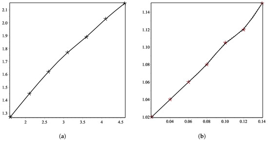
In this example we choose a positive data which is given in

Table 1. Positive data set of values.

$x_j^0$	1.6	2.1	2.6	3.1	3.6	4.1	4.6
$g_j^0$	1.27	1.45	1.62	1.77	1.89	2.03	2.15

, that fulfill the derived condition of positivity, i.e., it is easy to get that $Q^0=1.14$. We apply $FP$-scheme on this positive data five times. Graphical representation of this application is given in the Figure 1a. In this figure dotted line shows the initial positive data and the solid line represents the limit curve generated by $FP$-scheme. From the Figure 1a, it is clear that $FP$-scheme preserves positivity of initial data.

Example 2.

In this example we consider another positive data which is given in

Table 2. Positive data set of values.

$x_j^0$	0.02	0.04	0.06	0.08	0.10	0.12	0.14
$g_j^0$	1.02	1.04	1.06	1.08	1.105	1.12	1.15

, that fulfill the derived condition of positivity, i.e., it is easy to get that $Q^0=1.019$. We apply $FP$-scheme on this positive data five times. Graphical representation of this application is given in the Figure 1b. In this figure dotted line shows the initial positive data and the solid line represents the limit curve generated by $FP$-scheme. From the Figure 1b, it is clear that $FP$-scheme preserves positivity of initial data.

Example 3.

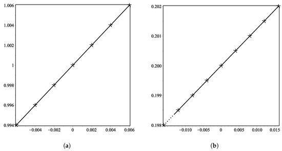
In this example we consider a monotonically increasing data which is given in

Table 3. Monotone data set of values.

$x_j^0$	−0.006	−0.004	−0.002	0	0.002	0.004	0.006
$g_j^0$	0.994	0.996	0.998	1	1.002	1.004	1.006

, that fulfill the derived condition of monotonicity, i.e., it is easy to get that $R^0=1$. We apply $FP$-scheme on this monotone data five times. Graphical representation of this application is given in the Figure 2a. In this figure dotted line shows the initial positive data and the solid line represents the limit curve generated by $FP$-scheme. From the Figure 2a, it is clear that the limit curve generated by the $FP$-scheme is also monotonically increasing.

Example 4.

In this example we consider another monotonically increasing data which is given in

Table 4. Monotone data set of values.

$x_j^0$	−0.006	−0.004	−0.002	0	0.002	0.004	0.006
$g_j^0$	0.1991	0.1994	0.1997	0.2000	0.2003	0.2006	0.2009

, that fulfill the derived condition of monotonicity, i.e., it is easy to get that $R^0=1$. We apply $FP$-scheme on this monotone data five times. Graphical representation of this application is given in the Figure 2b. In this figure dotted line shows the initial positive data and the solid line represents the limit curve generated by $FP$-scheme. From the Figure 2b, it is clear that the $FP$-scheme is capable of producing monotonically increasing limit curves.

Example 5.

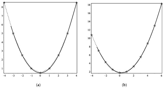
In this example we consider convex data from a convex function which is given in

Table 5. Convex data set of values.

$x_j^0$	−4	−3	−2	−1	0	1	2	3	4
$g_j^0$	8.5	5	2.5	1	0.5	1	2.5	5	8.5

, that fulfill the derived condition of convexity, i.e., it is easy to get that $S^0=1$. We apply $FP$-scheme on this convex data five times. Graphical representation of this application is given in the Figure 3a. In this figure dotted line shows the initial positive data and the solid line represents the limit curve generated by $FP$-scheme. From the Figure 3a, it is clear that the $FP$-scheme is capable of producing convex limit curves.

Example 6.

In this example we consider convex data from another convex function which is given in

Table 6. Convex data set of values.

$x_j^0$	−4	−3	−2	−1	0	1	2	3	4	5	6
$g_j^0$	10.75	7	4.25	2.5	1.75	2	3.25	5.5	8.75	13	18.25

, that fulfill the derived condition of convexity, i.e., it is easy to get that $S^0=1$. We apply $FP$-scheme on this convex data five times. Graphical representation of this application is given in the Figure 3b. In this figure dotted line shows the initial positive data and the solid line represents the limit curve generated by $FP$-scheme. From the Figure 3b, it is clear that the $FP$-scheme is capable of producing convex limit curves.

5.2. Conclusions

An approximating subdivision scheme with cubic precision and satisfying shape-preserving properties is a charming scheme for designers. We have presented analysis of some important shape-preserving properties of the $FP$-scheme, which make the scheme more efficient for application in geometric modeling. These properties assure that the shape preservation of the limit curve is an effective tool for modifying the $FP$-scheme for different requirements. We have shown that by taking initial control data positive, monotone and convex, the limit curves generated by the $FP$-scheme are also positive, monotone and convex. Also, we support our findings through several numerical examples. In future work, we are interested to analyze these shape-preserving properties in geometric notion. Extension of this work to case of surface is another future direction.

References

- Kuijt, F.; Damme, R.V. Shape preserving interpolatory subdivision schemes for nonuniform data. J. Approx. Theory 2002, 114, 1–32. [Google Scholar] [CrossRef]
- Cao, H.; Tan, J. A binary five-point relaxation subdivision scheme. J. Inf. Comp. Sci. 2013, 10, 5903–5910. [Google Scholar] [CrossRef]
- Tan, J.; Yao, Y.; Cao, H.; Zhang, L. Convexity preservation of five-point binary subdivision scheme with a parameter. Appl. Math. Comput. 2014, 245, 279–288. [Google Scholar] [CrossRef]
- Hassan, M.F.; Ivrissimitzis, I.; Dodgson, N.A.; Sabin, M.A. An interpolating 4-point C2 ternary stationary subdivision scheme. Comput. Aided Geom. Des. 2002, 19, 1–18. [Google Scholar] [CrossRef]
- Dyn, N.; Kuijt, F.; Levin, D.; van Damme, R. Convexity preservation of the four-point interpolatory subdivision scheme. Comput. Aided Geom. Des. 1999, 16, 789–792. [Google Scholar] [CrossRef]
- Dyn, N.; Levin, D.; Gregory, J.A. A 4-point interpolatory subdivision scheme for curve design. Comput. Aided Geom. Des. 1987, 4, 257–268. [Google Scholar] [CrossRef]
- Hao, Y.X.; Wang, R.H.; Li, C.J. Analsis of six point subdivision scheme. Appl. Math. Comput. 2011, 59, 2647–2657. [Google Scholar] [CrossRef]
- Kuijt, F.; van Damme, R. Monotonicity preserving interpolatory subdivision schemes. J. Comput. Appl. Math. 1999, 101, 203–229. [Google Scholar] [CrossRef]
- Kuijt, F.; van Damme, R. Convexity preserving interpolatory subdivision schemes. Constr. Approx. 1998, 14, 609–630. [Google Scholar] [CrossRef]
- Tan, J.; Zhuang, X.; Zhang, L. A new four-point shape-preserving C3 subdivision scheme. Comput. Aided Geom. Des. 2014, 31, 57–62. [Google Scholar] [CrossRef]
- Floater, M.; Beccari, C.; Cashman, T.; Romani, L. A smoothness criterion for monotonicity-preserving subdivision. Adv. Comput. Math. 2013, 39, 193–204. [Google Scholar] [CrossRef]
- Siddiqi, S.S.; Noreen, T. Convexity preservation of six point C2 interpolating subdivision scheme. Appl. Math. Comput. 2015, 265, 936–944. [Google Scholar] [CrossRef]
- Mustafa, G.; Ashraf, P. A new 6-point ternary interpolating subdivision scheme and its differentiability. J. Inf. Comput. Sci. 2010, 5, 199–210. [Google Scholar] [CrossRef]
- Albrecht, G.; Romani, L. Convexity preserving interpolatory subdivision with conic precision. Appl. Math. Comput. 2012, 219, 4049–4066. [Google Scholar] [CrossRef]
- Amat, S.; Donat, R.; Trillo, J.C. Proving convexity preserving properties of interpolatory subdivision schemes through reconstruction operators. Appl. Math. Comput. 2013, 219, 7413–7421. [Google Scholar] [CrossRef]
- Akram, G.; Bibi, K.; Rehan, K.; Siddiqi, S.S. Shape preservation of 4-point interpolating non-stationary subdivision scheme. J. Comput. Appl. Math. 2017, 319, 480–492. [Google Scholar] [CrossRef]
- Gabrielides, N.C.; Sapidis, N.S. C1 sign, monotonicity and convexity preserving hermite polynomial splines of variable degree. J. Comput. Appl. Math. 2018, 343, 662–707. [Google Scholar] [CrossRef]
- Mustafa, G.; Bashir, R. Univariate approximating schemes and their non-tensor product generalization. Open Math. 2018, 16, 1501–1518. [Google Scholar] [CrossRef]
- Ghaffar, A.; Ullah, Z.; Bari, M.; Nisar, K.S.; Al-Qurashi, M.M.; Baleanu, D. A new class of 2m-point binary non-stationary subdivision schemes. Adv. Differ. Equ. 2019, 325. [Google Scholar] [CrossRef]
- Asghar, M.; Mustafa, G. A Family of binary approximating subdivision schemes based on binomial distribution. Mehran Univ. Res. J. Eng. Technol. 2019, 38, 1087–1100. [Google Scholar] [CrossRef]
- Bibi, K.; Akram, G.; Rehan, K. Level set shape analysis of Binary 4-point non-stationary interpolating subdivision scheme. Int. J. Appl. Comput. Math. 2019, 5, 146. [Google Scholar] [CrossRef]
- Tan, J.; Wang, B.; Shi, J. A five-point subdivision scheme with two parameters and a four-point shape-preserving scheme. Math. Comput. Appl. 2017, 22, 22. [Google Scholar] [CrossRef]
- Dyn, N.; Iske, A.; Quak, E.; Floater, M.S. Tutorials on Multiresolution in Geometric Modelling. In Mathematics and Visualization; Summer School Lecture Notes Series; Springer Science & Business Media: Berlin, Germany, 2002. [Google Scholar]
- Mustafa, G.; Hashmi, M.S. Subdivision depth computation for n-ary subdivision curves/surfaces. Vis. Comput. 2010, 26, 841–851. [Google Scholar] [CrossRef]
- Shang, Y. Lack of Gromov-hyperbolicity in small-world networks. Cent. Eur. J. Math. 2011, 10, 1152–1158. [Google Scholar] [CrossRef]
- Mustafa, G.; Ghaffar, A.; Khan, F. The odd-point ternary approximating schemes. Am. J. Comput. Math. 2011, 1, 111–118. [Google Scholar] [CrossRef]
- Ghaffar, A.; Mustafa, G.; Qin, K. Unification and application of 3-point approximating subdivision schemes of varying arity. Open J. Appl. Sci. 2012, 2, 48–52. [Google Scholar] [CrossRef]
- Ghaffar, A.; Mustafa, G.; Qin, K. The 4-point 3-ary approximating subdivision scheme. Open J. Appl. Sci. 2013, 3, 106–111. [Google Scholar] [CrossRef]
- Mustafa, G.; Ghaffar, A.; Aslam, M. A subdivision-regularization framework for preventing over fitting of data by a model. AAM 2013, 8, 178–190. [Google Scholar]
- Siddiqi, S.S.; Younis, M. The Quaternary Interpolating Scheme for Geometric Design. Int. Sch. Res. Not. 2013, 2013, 434213. [Google Scholar] [CrossRef]
- Mustafa, G.; Ashraf, P.; Deng, J. Generalized and unified families of interpolating subdivision schemes. Numer. Math. Theory Methods Appl. 2014, 7, 193–213. [Google Scholar] [CrossRef]
- Rehan, K.; Siddiqi, S.S. A Family of Ternary Subdivision Schemes for Curves. Appl. Math. Comput. 2015, 270, 114–123. [Google Scholar] [CrossRef]
- Rehan, K.; Sabri, M.A. A combined ternary 4-point subdivision scheme. Appl. Math. Comput. 2016, 276, 278–283. [Google Scholar] [CrossRef]
- Peng, K.; Tan, J.; Li, Z.; Zhang, L. Fractal behavior of a ternary 4-point rational interpolation subdivision scheme. Math. Comput. Appl. 2018, 23, 65. [Google Scholar] [CrossRef]
- Zulkifli, N.A.B.; Karim, S.A.A.; Sarfraz, M.; Ghaffar, A.; Nisar, K.S. Image interpolation using a rational bi-cubic ball. Mathematics 2019, 7, 1045. [Google Scholar] [CrossRef]
- Ghaffar, A.; Ullah, Z.; Bari, M.; Nisar, K.S.; Baleanu, D. Family of odd point non-stationary subdivision schemes and their applications. Adv. Differ. Equ. 2019, 2019, 1–20. [Google Scholar] [CrossRef]
- Ghaffar, A.; Bari, M.; Ullah, Z.; Iqbal, M.; Nisar, K.S.; Baleanu, D. A New Class of 2q-Point Nonstationary Subdivision Schemes and Their Applications. Mathematics 2019, 7, 639. [Google Scholar] [CrossRef]
- Ghaffar, A.; Iqbal, M.; Bari, M.; Muhammad Hussain, S.; Manzoor, R.; Sooppy Nisar, K.; Baleanu, D. Construction and Application of Nine-Tic B-Spline Tensor Product SS. Mathematics 2019, 7, 675. [Google Scholar] [CrossRef]
- Zou, L.; Song, L.; Wang, X.; Chen, Y.; Zhang, C.; Tang, C. Bivariate thiele-like rational interpolation continued fractions with parameters based on virtual points. Mathematics 2020, 8, 71. [Google Scholar] [CrossRef]
- Shahzad, A.; Khan, F.; Ghaffar, A.; Mustafa, G.; Nisar, K.S.; Baleanu, D. A novel numerical algorithm to estimate the subdivision depth of binary subdivision schemes. Symmetry 2020, 12, 66. [Google Scholar] [CrossRef]
- Ashraf, P.; Sabir, M.; Ghaffar, A.; Nisar, K.S.; Khan, I. Shape-Preservation of Ternary Four-point Interpolating Non-stationary Subdivision Scheme. Front. Phys. 2019, 7, 241. [Google Scholar] [CrossRef]
- Ashraf, P.; Nawaz, B.; Baleanu, D.; Ghaffar, A.; Nisar, K.S.; Khan, A.A.; Akram, S. Analysis of geometric properties of ternary four-point rational interpolating subdivision scheme. Mathematics 2020, 8, 338. [Google Scholar] [CrossRef]
- Hussain, S.M.; Rehman, A.U.; Baleanu, D.; Ghaffar, A.; Nisar, K.S. Generalized 5-point approximating subdivision scheme of varying arity. Mathematics 2020, 8, 474. [Google Scholar] [CrossRef]
- Horman, K.; Sabin, M.A. A family of subdivision schemes with cubic percision. Comput. Aided Geom. Des. 2008, 25, 41–52. [Google Scholar] [CrossRef]
© 2020 by the authors. Licensee MDPI, Basel, Switzerland. This article is an open access article distributed under the terms and conditions of the Creative Commons Attribution (CC BY) license (http://creativecommons.org/licenses/by/4.0/).