Generalized 5-Point Approximating Subdivision Scheme of Varying Arity

Abstract

The Subdivision Schemes (SSs) have been the heart of Computer Aided Geometric Design (CAGD) almost from its origin, and various analyses of SSs have been conducted. SSs are commonly used in CAGD and several methods have been invented to design curves/surfaces produced by SSs to applied geometry. In this article, we consider an algorithm that generates the 5-point approximating subdivision scheme with varying arity. By applying the algorithm, we further discuss several properties: continuity, Hölder regularity, limit stencils, error bound, and shape of limit curves. The efficiency of the scheme is also depicted with assuming different values of shape parameter along with its application.

1. Introduction

Computer Aided Geometric Design (CAGD) deals with studies of curves and surfaces used in computer graphics, data structure, and computational algebra. In CAGD, geometric shapes are related to the mathematical representations that satisfy approximation and interpolation properties of curves and surfaces. Surface modeling is one of the important studies in the fields of CAGD and computer graphics. It links mathematical sciences with computer science and engineering such as the animation industry, automotive and industrial design, aerospace, mechanical engineering, and numerical computing. Subdivision is an interesting subject and one of the common tools in CAGD, which provides an elegant way for the description of curves and surfaces modeling. Initially, Rham [1] worked on subdivision schemes and made a scheme which generates a function with the first derivative. Similarly, Chaikin started work and used subdivision scheme to design a curve [2]. Subdivision schemes gained importance when scientists generalized the tensor product in an arbitrary topology. Doo and Catmull used the subdivision schemes to establish surface design and control meshes in an arbitrary topology [3,4]. Deslauriers and Dubuc formed a 4-point scheme [5]. Later, Dyn et al. [6] generalized the scheme of Dubuc and Deslauriers, known as the butterfly scheme, which is based on approximated schemes. Cai used a 4-point scheme with non-uniform control points to calculate convergence and error estimation. He illustrated that the curves and surfaces generated from 4-point schemes gave better results [7]. Hassan et al. [8,9] worked on arity and number of control points, whereas Mustafa and Xuefeng [10] worked on the scheme of Bajaj with new a parameter which controls the shape of models and gave more flexibility to design a model over the soft and rough mesh network. Similarly, Siddiqui and Ahmad [11] presented a 6-point subdivision scheme that gives better smoothness. Moreover, Hormann and Sabin [12] produced a family of subdivision schemes to calculate support size, Hölder regularity, precision set, and degree of polynomial curve. Khan and Mustafa [13] calculated an interpolating 6-point subdivision scheme for complex eigenvalues as well as worked on an approximating 4-point subdivision scheme. They showed that their scheme has higher smoothness and small support size as compared to other 4-point schemes [14]. Mustafa et al. [15] worked on the m-point approximating subdivision schemes and illustrated that their schemes have higher smoothness as compared to other subdivision schemes. Siddiqi and Rehan [16] worked on a 4-point binary scheme to generate the family of curves. They introduced a scheme for $C^1$ continuity to generate a curve called corner cutting. Mustafa et al. [17] further worked on odd-point ternary approximating subdivision schemes and developed a formula to generalize them. Later, Ghaffar et al. [18] considered 3-point approximating subdivision schemes and observed that the given approach is more universal and is applied to schemes of arbitrary arity. Ghaffar et al. [19] introduced a general formula for 4-point a-ary approximating subdivision scheme for curve designing for any arity $a\ge 2$.

In addition, Mustafa et al. [20] worked over odd point ternary families of approximating subdivision schemes and showed that their schemes have high smoothness. They also worked on subdivision regularization, in which they showed that unified frame work can work well for both curve fitting and noise removal. They generalized unified families of interpolating subdivision schemes of $2n$-point and $(2n-1)$-point p-ary which generate Lagrange’s polynomial for $n\ge 2$ and $p\ge 3$, presented in [21]. In 2013, Younus and Siddiqi [22] established an algorithm based on Quaternary-point for $(m>1)$ approximating subdivision scheme which has high smoothness and small support. Rehan et al. [23] discussed the continuity of a new class of 3-point ternary schemes and generated limiting curves using the proposed schemes. They also proposed a 4-point ternary scheme which creates $C^0$ interpolating and $C^1,C^2,C^3$ approximating limiting curves, described in [24]. For other recent work on this topic, we may refer to [25,26,27,28,29] and references therein.

The above-mentioned literature shows limited knowledge about the arity of the SSs. This motivated us to construct a unified 5-point approximating SS of varying arity with the shape controlling parameter. To show the performance of the schemes, we analyze the geometric properties such as continuity, Hölder regularity, and Limit stencils. Moreover, the limit curves with the specific value of shape control parameter w are depicted by the significant application of derived conditions on the initial data. The rest of the paper is organized as follows. The preliminaries regarding SSs are presented in Section 2. In Section 3, we analyze the geometric properties of the proposed schemes. The results and discussion are presented in Section 4. Some example are considered in this section to show the efficiency of the schemes. Finally, the concluding remarks are given in final section.

2. Preliminaries

In this section, we recall some well known concepts and basic results.

Definition 1.

A curve which is generated by applying a subdivision operator repeatedly to a given polygon is known as subdivision curve.

Definition 2.

If the mask of the scheme is similar for all points of the control polygon, the scheme is known as stationary.

Definition 3.

If the mask of the scheme is not similar for all points of the control polygon, the scheme is known as non-stationary.

Definition 4.

In an approximating scheme, every data point that belongs to a function generated at stage k does not belong at stage $k+1$.

Definition 5.

In an interpolating scheme, every data point belongs to a function at both stages/levels k and $k+1$.

Theorem 1.

[30] ${\mathit{S}}_a$ scheme converges iff the scheme ${\mathit{S}}_c$ is contractive. ${\mathit{S}}_c$ is contractive if $\parallel c_l\parallel <1$ for some $l>0$ with $\parallel c_l\parallel =max{\sum }_j|c_{k-2_j^l}^l|:0\le k<2^l$, where $c_j^l$ are the coefficients of the scheme $S_c^l$ with Laurent polynomial $c^l\left(x\right)=c\left(x\right)c\left(x^2\right)\dots c(x^{2^l-1})$.

Theorem 2.

[30] If ${\mathit{S}}_b$ converges, then the limit curves of the scheme ${\mathit{S}}_a$ with Laurent polynomial $a\left(x\right)={\left(\frac{1+x}{2}\right)}^{m}b\left(x\right)$ are $C^m$ continuous, where ${\mathit{S}}_b$ is the scheme for the mth divided differences.

Theorem 3.

[30] The scheme ${\mathit{S}}_a$ with Laurent polynomial $\alpha \left(x\right)={\left(\frac{1+x}{2}\right)}^{m}b\left(x\right)$ generates limit curves with Hölder regularity $r\ge m-{log}_2\frac{\parallel b^l\parallel }{l}$ for any l.

An a-ary scheme is said to be linear if it generates level $k+1$ from level k with linear combination of control points, that is for all ‘k’ and ‘j’, there exists sets of real numbers known as masks ${\mathbf{a}}^k=\left\{a^k\right\}$ such that

$${\lambda }_j^{k+1}=\sum _{i\in \mathbb{Z}}{a}_{j-ni}^k{\lambda }_i^k.$$

If the mask of the scheme is independent of k, then the scheme has finite support. Similarly, if the mask is independent of ‘j’, that is each refinement rule operates in the same way at all locations, then the scheme is known as uniform.

A general formula for the mask of the proposed scheme is defined as

$${\alpha }_5^a\left(x\right)=\frac{1}{2a^4}{\left(\frac{1-x^a}{1-x}\right)}^4\sum _{i=0}^4\left(\genfrac{}{}{0pt}{}{4}{i}\right){\omega }_i$$

(1)

and

$$\sum _{i=0}^4\frac{a}{8}\left(\genfrac{}{}{0pt}{}{4}{i}\right){\omega }_i=a;\hspace{1em}\mathrm{where} {\omega }_j={\omega }_{3-j} \mathrm{and} j=0,1,2,$$

(2)

where w is called the shape controlling parameter and it is used to control the shape of the control of the polygon.

3. The 5-Point Approximating Schemes

This section consists of different 5-point approximating schemes together with the properties: convergence criteria, continuity, Hölder regularity, and limit stencils.

3.1. 5-Point Binary Approximating Scheme

By substituting $a=2$ into Equations (1) and (2), we can get the scheme in the form

$$\begin{array}{ccc}\hfill {\lambda }_{2i}^{j+1}& =& \frac{1}{256}\left[(4+5\omega ){\lambda }_{i-2}^j+84{\lambda }_{i-1}^j+(140-14\omega ){\lambda }_i^j+(28+8\omega ){\lambda }_{i+1}^j+\omega {\lambda }_{i+2}^j\right],\hfill \\ \hfill {\lambda }_{2i+1}^{j+1}& =& \frac{1}{256}\left[\omega {\lambda }_{i-2}^j+(28+8\omega ){\lambda }_{i-1}^j+(140-14\omega ){\lambda }_i^j+84{\lambda }_{i+1}^j+(4+5\omega ){\lambda }_{i+2}^j\right],\hfill \end{array}$$

(3)

called 5-point binary approximating scheme.

3.1.1. Convergence Criteria

The mask of the binary scheme using Equation (3) may be written as

$$\begin{array}{ccc}\hfill a& =& \frac{1}{256}\left\{\omega ,(4+5\omega ),(28+8\omega ),84,(140-14\omega ),(140-14\omega ),84,(28+8\omega ),(4+5\omega ),\omega \right\}.\hfill \end{array}$$

(4)

The even and odd stencil of the above scheme may be written as $\frac{(\omega ,(28+8\omega ),(140-14\omega ),84,(4+5\omega \left)\right)}{256}$ and the sum of the coefficients may be written as

$$\begin{array}{c}\hfill \frac{\{\omega +(28+8\omega )+(140-14\omega )+84+(4+5\omega \left)\right\}}{256}=1,\end{array}$$

which shows the convergence condition of the scheme.

The Laurent polynomial $a\left(x\right)$ of Equation (3) takes the form

$$\begin{array}{ccc}\hfill a\left(x\right)& =& \frac{1}{256}\left\{\omega +(4+5\omega )x+(28+8\omega )x^2+84x^3+(140-14\omega )x^4+(140-14\omega )x^5\right.\hfill \\ \hfill & & \left.+84x^6+(28+8\omega )x^7+(4+5\omega )x^8+\omega x^9\right\}.\hfill \end{array}$$

(5)

After simplification, Equation (5) becomes

$$\begin{array}{ccc}\hfill a\left(x\right)& =& {\left(\frac{1+x}{2}\right)}^{7}b\left(x\right),\hfill \end{array}$$

(6)

where

$$\begin{array}{ccc}\hfill b\left(x\right)& =& \frac{\left(\omega x^2+\left(4-2\omega \right)x+\omega \right)}{2}.\hfill \end{array}$$

3.1.2. Continuity

To find continuity of the scheme, Equation (6) gives the Laurent polynomial of the form

$$\begin{array}{ccc}\hfill a\left(x\right)& =& \left(\frac{1+x}{2}\right)b_1\left(x\right),\hfill \end{array}$$

(7)

where

$$\begin{array}{ccc}\hfill b_1\left(x\right)& =& \left\{\frac{\omega x^8}{128}+\left(\frac{\omega }{32}+\frac{1}{32}\right)x^7+\left(\frac{\omega }{32}+\frac{3}{16}\right)x^6+\left(\frac{15}{32}-\frac{\omega }{32}\right)x^5\right.\hfill \\ \hfill & & \left.+\left(\frac{5}{8}-\frac{5\omega }{64}\right)x^4+\left(\frac{15}{32}-\frac{\omega }{32}\right)x^3+\left(\frac{\omega }{32}+\frac{3}{16}\right)x^2+\left(\frac{\omega }{32}+\frac{1}{32}\right)x+\frac{\omega }{128}\right\}.\hfill \end{array}$$

$C^0$ continuity of the scheme $S_a$ analogous to $a\left(x\right)$, $b_1\left(x\right)$ should be convergent, where $b_1\left(x\right)$ should satisfy Theorem 1 with the given condition ${∥\frac{1}{2}\left(S_{b_1}\right)∥}_{\infty }<1$. From Theorem 1, for $-9<\omega <72/5$, we extract

$$\begin{array}{ccc}\hfill {∥\frac{1}{2}\left(S_{b_1}\right)∥}_{\infty }& =& \frac{1}{2}\max \left\{\left|\frac{\omega }{32}+\frac{1}{32}\right|+2\left|\frac{\omega }{32}-\frac{15}{32}\right| \frac{\left|\omega \right|}{128}+\left|\frac{\omega }{64}+\frac{3}{32}\right|+\left|\frac{5\omega }{128}-\frac{5}{16}\right|\right\}<1.\hfill \end{array}$$

The given condition satisfies Theorem 1, thus it must satisfy Theorem 2. This shows that the 5-point scheme is $C^0$ continuous.

For $C^1$ continuity, Equation (6) takes the form

$$\begin{array}{c}\hfill b_2\left(x\right)=\left(\frac{2}{1+x}\right)b_1\left(x\right),\end{array}$$

or

$$\begin{array}{ccc}\hfill b_2\left(x\right)& =& \left\{\frac{\omega x^7}{64}+\left(\frac{3\omega }{64}+\frac{1}{16}\right)x^6+\left(\frac{\omega }{64}+\frac{5}{16}\right)x^5+\left(-\frac{5\omega }{64}+\frac{5}{8}\right)x^4\right.\hfill \\ \hfill & & \left.+\left(-\frac{5\omega }{64}+\frac{5}{8}\right)x^3+\left(\frac{\omega }{64}+\frac{5}{16}\right)x^2+\left(\frac{3\omega }{64}+\frac{1}{16}\right)x+\frac{\omega }{64}\right\},\hfill \end{array}$$

which satisfies Theorem 1 with the given condition ${∥\frac{1}{2}\left(S_{b_2}\right)∥}_{\infty }<1$. From Theorem 1, for $-9<\omega <72/5$, we extract

$$\begin{array}{ccc}\hfill {∥\frac{1}{2}\left(S_{b_2}\right)∥}_{\infty }& =& \frac{1}{2}\max \left\{\frac{\left|\omega \right|}{64}+\left|\frac{\omega }{64}+\frac{5}{16}\right|+\left|\frac{5\omega }{64}-\frac{5}{8}\right|+\left|\frac{3\omega }{64}+\frac{1}{16}\right|\right\}<1,\hfill \end{array}$$

which shows that the scheme is $C^1$ continuous.

For $C^2$ continuity, Equation (6) may be written as

$$\begin{array}{c}\hfill b_3\left(x\right)=\left(\frac{2}{1+x}\right)b_2\left(x\right),\end{array}$$

or

$$\begin{array}{ccc}\hfill b_3\left(x\right)& =& \left\{\frac{1}{32}\omega x^6+\left(\frac{\omega }{16}+\frac{1}{8}\right)x^5+\left(\frac{-\omega }{32}+\frac{1}{2}\right)x^4+\left(\frac{-\omega }{8}+\frac{3}{4}\right)x^3\right.\hfill \\ \hfill & & \left.+\left(\frac{-\omega }{32}+\frac{1}{2}\right)x^2+\left(\frac{\omega }{16}+\frac{1}{8}\right)x+\frac{\omega }{32}\right\},\hfill \end{array}$$

which satisfies Theorem 1 with the given condition ${∥\frac{1}{2}\left(S_{b_3}\right)∥}_{\infty }<1$. From Theorem 1, for $-6<\omega <10$, we can get

$$\begin{array}{ccc}\hfill {∥\frac{1}{2}\left(S_{b_3}\right)∥}_{\infty }& =& \frac{1}{2}\max \left\{\frac{1}{16}\left|\omega \right|+2\left|\frac{\omega }{32}-\frac{1}{2}\right|+2\left|\frac{\omega }{16}+\frac{1}{8}\right|+\left|\frac{\omega }{8}-\frac{3}{4}\right|\right\}<1.\hfill \end{array}$$

Hence, the scheme is $C^2$ continuous.

For $C^3$ continuity, Equation (6) takes the form

$$\begin{array}{c}\hfill b_4\left(x\right)=\left(\frac{2}{1+x}\right)b_3\left(x\right),\end{array}$$

or

$$\begin{array}{ccc}\hfill b_4\left(x\right)& =& \left\{\frac{1}{16}\omega x^5+\left(\frac{\omega }{16}+\frac{1}{4}\right)x^4+\left(\frac{-\omega }{8}+\frac{3}{4}\right)x^3+\left(\frac{-\omega }{8}+\frac{3}{4}\right)x^2+\left(\frac{\omega }{16}+\frac{1}{4}\right)x+\frac{\omega }{16}\right\},\hfill \end{array}$$

which satisfies Theorem 1 with the given condition ${∥\frac{1}{2}\left(S_{b_4}\right)∥}_{\infty }<1$. From Theorem 1, for $-6<\omega <10$, we extract

$$\begin{array}{ccc}\hfill {∥\frac{1}{2}\left(S_{b_4}\right)∥}_{\infty }& =& \frac{1}{2}\max \left\{\frac{1}{16}\left|\omega \right|+\left|\frac{\omega }{8}-\frac{3}{4}\right|+\left|\frac{\omega }{16}+\frac{1}{4}\right|\right\}<1,\hfill \end{array}$$

which shows that the scheme is $C^3$ continuous.

For $C^4$ continuity, Equation (6) may be written as

$$\begin{array}{c}\hfill b_5\left(x\right)=\left(\frac{2}{1+x}\right)b_4\left(x\right),\end{array}$$

or

$$\begin{array}{ccc}\hfill b_5\left(x\right)& =& \left\{\frac{1}{8}\omega x^4+\frac{1}{2}{x}^3+\left(-\frac{\omega }{4}+1\right)x^2+\frac{x}{2}+\frac{\omega }{8}\right\},\hfill \end{array}$$

with the given condition ${∥\frac{1}{2}\left(S_{b_5}\right)∥}_{\infty }<1$. Thus, from Theorem 1, for $-2<\omega <6$, we can get

$$\begin{array}{ccc}\hfill {∥\frac{1}{2}\left(S_{b_5}\right)∥}_{\infty }& =& \frac{1}{2}\max \left\{\frac{1}{4}\left|\omega \right|+\left|\frac{\omega }{4}-1\right|\right\}<1.\hfill \end{array}$$

This satisfies Theorem 1, thus it must satisfy Theorem 2. Thus, the scheme is $C^4$ continuous.

For $C^5$ continuity, Equation (6) may be written as

$$\begin{array}{c}\hfill b_6\left(x\right)=\left(\frac{2}{1+x}\right)b_5\left(x\right),\end{array}$$

or

$$\begin{array}{ccc}\hfill b_6\left(x\right)& =& \left\{\frac{1}{4}\omega x^3+\left(\frac{-\omega }{4}+1\right)x^2+\left(\frac{-\omega }{4}+1\right)x+\frac{\omega }{4}\right\},\hfill \end{array}$$

with the given condition ${∥\frac{1}{2}\left(S_{b_6}\right)∥}_{\infty }<1$. From Theorem 1, for $-2<\omega <6$, we extract

$$\begin{array}{ccc}\hfill {∥\frac{1}{2}\left(S_{b_6}\right)∥}_{\infty }& =& \frac{1}{2}\max \left\{\frac{1}{4}\left|\omega \right|+\left|\frac{\omega }{4}-1\right|\right\}<1,\hfill \end{array}$$

which shows that the scheme is $C^5$ continuous.

For $C^6$ continuity, Equation (6) may be written as

$$\begin{array}{c}\hfill b_7\left(x\right)=\left(\frac{2}{1+x}\right)b_6\left(x\right),\end{array}$$

or

$$\begin{array}{ccc}\hfill b_7\left(x\right)& =& \left\{\frac{1}{2}\omega x^2+\left(-\omega +2\right)x+\frac{\omega }{2}\right\},\hfill \end{array}$$

(8)

with the given condition ${∥\frac{1}{2}\left(S_{b_7}\right)∥}_{\infty }<1$. If we extract for $0<\omega <2$

$$\begin{array}{ccc}\hfill {∥\frac{1}{2}\left(S_{b_7}\right)∥}_{\infty }& =& \frac{1}{2}\max \left\{\left|\omega \right|\right\}<1,\hfill \end{array}$$

The given condition satisfies Theorem 1, thus it must satisfy Theorem 2, which shows $C^6$ continuity of the scheme.

Similarly, for $C^7$ continuity we substitute $\omega =1$ in Equation (6) and get

$$\begin{array}{ccc}\hfill b_7\left(x\right)& =& \left\{\frac{1}{2}(x+1)(x+1)\right\},\hfill \end{array}$$

this implies that

$$\begin{array}{ccc}\hfill b_8\left(x\right)& =& \left\{\left(\frac{2}{1+x}\right)\right\}{b}_7\left(x\right).\hfill \end{array}$$

or

$$\begin{array}{ccc}\hfill b_8\left(x\right)& =& \left\{(x+1)\right\}.\hfill \end{array}$$

From Theorem 2, we have

$$\begin{array}{ccc}\hfill {∥\frac{1}{2}\left(S_{b_8}\right)∥}_{\infty }& =& \frac{1}{2}\max \left\{1,1\right\}<1.\hfill \end{array}$$

Therefore, the scheme is $C^7$ continuous.

3.1.3. Hölder Regularity

We use Theorem 3 to find Hölder regularity of the scheme. The Laurent polynomial of the binary scheme using Equation (3) may be written as

$$\begin{array}{ccc}\hfill a\left(x\right)& =& \frac{1}{256}\left\{\omega +(4+5\omega )x+(28+8\omega )x^2+84x^3+(140-14\omega )x^4+(140-14\omega )x^5\right.\hfill \\ \hfill & & \left.+84x^6+(28+8\omega )x^7+(4+5\omega )x^8+\omega x^9\right\}.\hfill \end{array}$$

(9)

or

$$\begin{array}{ccc}\hfill a\left(x\right)& =& {\left(\frac{1+x}{2}\right)}^{7}b\left(x\right),\hfill \end{array}$$

(10)

where

$$\begin{array}{ccc}\hfill b\left(x\right)& =& \frac{\left(\omega x^2+\left(4-2\omega \right)x+\omega \right)}{2}.\hfill \end{array}$$

(11)

If $\omega =1$, we can get $b=2$. Using Theorem 3 with $m=7$ and $b=2$, we have $r\ge 7-{log}_2\left(2\right)$ = 6.

3.1.4. Limit Stencils

The matrix form of the scheme using Equation (3) for $w=1$ has the form

$$\begin{array}{c}\hfill \left[\begin{array}{c}{\lambda }_{-3}^j\\ {\lambda }_{-2}^j\\ {\lambda }_{-1}^j\\ {\lambda }_0^j\\ {\lambda }_1^j\\ {\lambda }_2^j\\ {\lambda }_3^j\\ {\lambda }_4^j\end{array}\right]=\left[\begin{array}{cccccccc}\frac{9}{256}& \frac{21}{64}& \frac{63}{128}& \frac{9}{64}& \frac{1}{256}& 0& 0& 0\\ \frac{1}{256}& \frac{9}{64}& \frac{63}{128}& \frac{21}{64}& \frac{9}{256}& 0& 0& 0\\ 0& \frac{9}{256}& \frac{21}{64}& \frac{63}{128}& \frac{9}{64}& \frac{1}{256}& 0& 0\\ 0& \frac{1}{256}& \frac{9}{64}& \frac{63}{128}& \frac{21}{64}& \frac{9}{256}& 0& 0\\ 0& 0& \frac{9}{256}& \frac{21}{64}& \frac{63}{128}& \frac{9}{64}& \frac{1}{256}& 0\\ 0& 0& \frac{1}{256}& \frac{9}{64}& \frac{63}{128}& \frac{21}{64}& \frac{9}{256}& 0\\ 0& 0& 0& \frac{9}{256}& \frac{21}{64}& \frac{63}{128}& \frac{9}{64}& \frac{1}{256}\\ 0& 0& 0& \frac{1}{256}& \frac{9}{64}& \frac{63}{128}& \frac{21}{64}& \frac{9}{256}\end{array}\right]\left[\begin{array}{c}{\lambda }_{-3}^{j-1}\\ {\lambda }_{-2}^{j-1}\\ {\lambda }_{-1}^{j-1}\\ {\lambda }_0^{j-1}\\ {\lambda }_1^{j-1}\\ {\lambda }_2^{j-1}\\ {\lambda }_3^{j-1}\\ {\lambda }_4^{j-1}\end{array}\right]\end{array}$$

and the local subdivision matrix

$$\begin{array}{c}\hfill X=\left[\begin{array}{cccccccc}\frac{9}{256}& \frac{21}{64}& \frac{63}{128}& \frac{9}{64}& \frac{1}{256}& 0& 0& 0\\ \frac{1}{256}& \frac{9}{64}& \frac{63}{128}& \frac{21}{64}& \frac{9}{256}& 0& 0& 0\\ 0& \frac{9}{256}& \frac{21}{64}& \frac{63}{128}& \frac{9}{64}& \frac{1}{256}& 0& 0\\ 0& \frac{1}{256}& \frac{9}{64}& \frac{63}{128}& \frac{21}{64}& \frac{9}{256}& 0& 0\\ 0& 0& \frac{9}{256}& \frac{21}{64}& \frac{63}{128}& \frac{9}{64}& \frac{1}{256}& 0\\ 0& 0& \frac{1}{256}& \frac{9}{64}& \frac{63}{128}& \frac{21}{64}& \frac{9}{256}& 0\\ 0& 0& 0& \frac{9}{256}& \frac{21}{64}& \frac{63}{128}& \frac{9}{64}& \frac{1}{256}\\ 0& 0& 0& \frac{1}{256}& \frac{9}{64}& \frac{63}{128}& \frac{21}{64}& \frac{9}{256}\end{array}\right],\end{array}$$

which shows that the size of the invariant neighborhood is 8. After simplification, matrix X has eigenvalues $\lambda =1,\frac{1}{2},\frac{1}{4},\frac{1}{8},\frac{1}{16},\frac{1}{32},\frac{1}{64},\frac{1}{128}$ and eigenvectors

$$\begin{array}{c}\hfill \left[\begin{array}{c}1\\ \frac{1}{2}\\ \frac{1}{4}\\ \frac{1}{8}\\ \frac{1}{16}\\ \frac{1}{32}\\ \frac{1}{64}\\ \frac{1}{128}\end{array}\right]\left[\begin{array}{cccccccc}1& 1& -1& 1& -1& -1& -1& 1\\ \frac{127}{967}& \frac{11}{23}& \frac{1}{7}& -\frac{29}{363}& -\frac{2}{7}& -\frac{5}{469}& -\frac{5}{7}& 1\\ -\frac{33}{967}& \frac{3}{23}& -\frac{1}{21}& \frac{47}{3267}& 0& \frac{9}{469}& -\frac{3}{7}& 1\\ \frac{7}{967}& -\frac{1}{23}& \frac{1}{35}& -\frac{1}{363}& \frac{1}{35}& -\frac{1}{67}& -\frac{1}{7}& 1\\ \frac{7}{967}& -\frac{1}{23}& -\frac{1}{35}& -\frac{1}{363}& -\frac{1}{35}& \frac{1}{67}& \frac{1}{7}& 1\\ -\frac{33}{967}& \frac{3}{23}& \frac{1}{21}& \frac{47}{3267}& 0& -\frac{9}{469}& \frac{3}{7}& 1\\ \frac{127}{967}& \frac{11}{23}& -\frac{1}{7}& -\frac{29}{363}& \frac{2}{7}& \frac{5}{469}& \frac{5}{7}& 1\\ 1& 1& 1& 1& 1& 1& 1& 1\end{array}\right].\end{array}$$

Let

$$\begin{array}{c}\hfill Y=\left[\begin{array}{cccccccc}1& 1& -1& 1& -1& -1& -1& 1\\ \frac{127}{967}& \frac{11}{23}& \frac{1}{7}& -\frac{29}{363}& -\frac{2}{7}& -\frac{5}{469}& -\frac{5}{7}& 1\\ -\frac{33}{967}& \frac{3}{23}& -\frac{1}{21}& \frac{47}{3267}& 0& \frac{9}{469}& -\frac{3}{7}& 1\\ \frac{7}{967}& -\frac{1}{23}& \frac{1}{35}& -\frac{1}{363}& \frac{1}{35}& -\frac{1}{67}& -\frac{1}{7}& 1\\ \frac{7}{967}& -\frac{1}{23}& -\frac{1}{35}& -\frac{1}{363}& -\frac{1}{35}& \frac{1}{67}& \frac{1}{7}& 1\\ -\frac{33}{967}& \frac{3}{23}& \frac{1}{21}& \frac{47}{3267}& 0& -\frac{9}{469}& \frac{3}{7}& 1\\ \frac{127}{967}& \frac{11}{23}& -\frac{1}{7}& -\frac{29}{363}& \frac{2}{7}& \frac{5}{469}& \frac{5}{7}& 1\\ 1& 1& 1& 1& 1& 1& 1& 1\end{array}\right].\end{array}$$

Thus, the decomposition of the local subdivision matrix X has the form $X=Y\wedge Y^{-1}$.

$$\begin{array}{c}\hfill \left[\begin{array}{cccccccc}\frac{9}{256}& \frac{21}{64}& \frac{63}{128}& \frac{9}{64}& \frac{1}{256}& 0& 0& 0\\ \frac{1}{256}& \frac{9}{64}& \frac{63}{128}& \frac{21}{64}& \frac{9}{256}& 0& 0& 0\\ 0& \frac{9}{256}& \frac{21}{64}& \frac{63}{128}& \frac{9}{64}& \frac{1}{256}& 0& 0\\ 0& \frac{1}{256}& \frac{9}{64}& \frac{63}{128}& \frac{21}{64}& \frac{9}{256}& 0& 0\\ 0& 0& \frac{9}{256}& \frac{21}{64}& \frac{63}{128}& \frac{9}{64}& \frac{1}{256}& 0\\ 0& 0& \frac{1}{256}& \frac{9}{64}& \frac{63}{128}& \frac{21}{64}& \frac{9}{256}& 0\\ 0& 0& 0& \frac{9}{256}& \frac{21}{64}& \frac{63}{128}& \frac{9}{64}& \frac{1}{256}\\ 0& 0& 0& \frac{1}{256}& \frac{9}{64}& \frac{63}{128}& \frac{21}{64}& \frac{9}{256}\end{array}\right]=\left[\begin{array}{cccccccc}1& 1& -1& 1& -1& -1& -1& 1\\ \frac{127}{967}& \frac{11}{23}& \frac{1}{7}& -\frac{29}{363}& -\frac{2}{7}& -\frac{5}{469}& -\frac{5}{7}& 1\\ -\frac{33}{967}& \frac{3}{23}& -\frac{1}{21}& \frac{47}{3267}& 0& \frac{9}{469}& -\frac{3}{7}& 1\\ \frac{7}{967}& -\frac{1}{23}& \frac{1}{35}& -\frac{1}{363}& \frac{1}{35}& -\frac{1}{67}& -\frac{1}{7}& 1\\ \frac{7}{967}& -\frac{1}{23}& -\frac{1}{35}& -\frac{1}{363}& -\frac{1}{35}& \frac{1}{67}& \frac{1}{7}& 1\\ -\frac{33}{967}& \frac{3}{23}& \frac{1}{21}& \frac{47}{3267}& 0& -\frac{9}{469}& \frac{3}{7}& 1\\ \frac{127}{967}& \frac{11}{23}& -\frac{1}{7}& -\frac{29}{363}& \frac{2}{7}& \frac{5}{469}& \frac{5}{7}& 1\\ 1& 1& 1& 1& 1& 1& 1& 1\end{array}\right]\end{array}$$

$$\begin{array}{c}\hfill \left[\begin{array}{cccccccc}1& 0& 0& 0& 0& 0& 0& 0\\ 0& \frac{1}{2}& 0& 0& 0& 0& 0& 0\\ 0& 0& \frac{1}{4}& 0& 0& 0& 0& 0\\ 0& 0& 0& \frac{1}{8}& 0& 0& 0& 0\\ 0& 0& 0& 0& \frac{1}{16}& 0& 0& 0\\ 0& 0& 0& 0& 0& \frac{1}{32}& 0& 0\\ 0& 0& 0& 0& 0& 0& \frac{1}{64}& 0\\ 0& 0& 0& 0& 0& 0& 0& \frac{1}{128}\end{array}\right]\left[\begin{array}{cccccccc}\frac{967}{5760}& \frac{6769}{5760}& -\frac{2901}{640}& \frac{18,373}{5760}& \frac{18,373}{5760}& -\frac{2901}{640}& \frac{6769}{5760}& \frac{967}{5760}\\ \frac{23}{2880}& \frac{253}{576}& \frac{483}{320}& -\frac{1127}{576}& -\frac{1127}{576}& \frac{483}{320}& \frac{253}{576}& \frac{23}{2880}\\ -\frac{1}{8}& \frac{7}{8}& -\frac{21}{8}& \frac{35}{8}& -\frac{35}{8}& \frac{21}{8}& -\frac{7}{8}& \frac{1}{8}\\ \frac{363}{1120}& -\frac{363}{224}& \frac{3267}{1120}& -\frac{363}{224}& -\frac{363}{224}& \frac{3267}{1120}& -\frac{363}{224}& \frac{363}{1120}\\ -\frac{7}{144}& -\frac{161}{144}& \frac{7}{16}& \frac{665}{144}& -\frac{665}{144}& -\frac{7}{16}& \frac{161}{144}& \frac{7}{144}\\ -\frac{469}{1440}& \frac{469}{1440}& \frac{469}{160}& -\frac{2345}{288}& \frac{2345}{288}& -\frac{469}{160}& -\frac{469}{1440}& \frac{469}{1440}\\ -\frac{1}{1440}& -\frac{119}{1440}& -\frac{119}{160}& -\frac{245}{288}& \frac{245}{288}& \frac{119}{160}& \frac{119}{1440}& \frac{1}{1440}\\ \frac{1}{40,320}& \frac{247}{40,320}& \frac{477}{4480}& \frac{15,619}{40,320}& \frac{15,619}{40,320}& \frac{477}{4480}& \frac{247}{40,320}& \frac{1}{40,320}\end{array}\right].\end{array}$$

Using diagonalization $\wedge =X^{-1}AX$, where as ∧ represents diagonal matrix and $A=X\wedge X^{-1}$. In addition, $X=Y\wedge Y^{-1}$ implies that $X^j=Y{\wedge }^j{Y}^{-1}$ and $\wedge =X^{-1}AX$ implies that $A^j=X{\wedge }^j{X}^{-1}$.

Since the ∧ is diagonal matrix and also the power of a diagonal matrix is equal to the power of each diagonal element. Therefore,

$$\begin{array}{c}\hfill {\wedge }^j=\left[\begin{array}{cccccccc}{\left(1\right)}^j& 0& 0& 0& 0& 0& 0& 0\\ 0& {\left(\frac{1}{2}\right)}^j& 0& 0& 0& 0& 0& 0\\ 0& 0& {\left(\frac{1}{4}\right)}^j& 0& 0& 0& 0& 0\\ 0& 0& 0& {\left(\frac{1}{8}\right)}^j& 0& 0& 0& 0\\ 0& 0& 0& 0& {\left(\frac{1}{16}\right)}^j& 0& 0& 0\\ 0& 0& 0& 0& 0& {\left(\frac{1}{32}\right)}^j& 0& 0\\ 0& 0& 0& 0& 0& 0& {\left(\frac{1}{64}\right)}^j& 0\\ 0& 0& 0& 0& 0& 0& 0& {\left(\frac{1}{128}\right)}^j\end{array}\right]\end{array}$$

Since $X^j=Y{\wedge }^j{Y}^{-1}$, by substituting the eigen decomposition of X, we get ${\lambda }^j=X{\lambda }^{j-1}=X\left(X{\lambda }^{j-2}\right)=X^2{\lambda }^{j-2}$ … up to ${\lambda }^j=X^j{\lambda }^0$, or ${\lambda }^j=\left(Y{\wedge }^j{Y}^{-1}\right){\lambda }^0$. Taking ${lim}_{j\to \infty }$${\lambda }^{\infty }={lim}_{j\to \infty }{X}^j{\lambda }^0=X^{\infty }{\lambda }^0$ or ${\lambda }^{\infty }=Y{\wedge }^{\infty }{Y}^{-1}{\lambda }^0$.

$$\begin{array}{c}\hfill \left[\begin{array}{c}{\lambda }_{-3}^{j-1}\\ {\lambda }_{-2}^j\\ {\lambda }_{-1}^j\\ {\lambda }_0^j\\ {\lambda }_1^j\\ {\lambda }_2^j\\ {\lambda }_3^j\\ {\lambda }_4^{j-1}\end{array}\right]=\left[\begin{array}{cccccccc}\frac{9}{256}& \frac{21}{64}& \frac{63}{128}& \frac{9}{64}& \frac{1}{256}& 0& 0& 0\\ \frac{1}{256}& \frac{9}{64}& \frac{63}{128}& \frac{21}{64}& \frac{9}{256}& 0& 0& 0\\ 0& \frac{9}{256}& \frac{21}{64}& \frac{63}{128}& \frac{9}{64}& \frac{1}{256}& 0& 0\\ 0& \frac{1}{256}& \frac{9}{64}& \frac{63}{128}& \frac{21}{64}& \frac{9}{256}& 0& 0\\ 0& 0& \frac{9}{256}& \frac{21}{64}& \frac{63}{128}& \frac{9}{64}& \frac{1}{256}& 0\\ 0& 0& \frac{1}{256}& \frac{9}{64}& \frac{63}{128}& \frac{21}{64}& \frac{9}{256}& 0\\ 0& 0& 0& \frac{9}{256}& \frac{21}{64}& \frac{63}{128}& \frac{9}{64}& \frac{1}{256}\\ 0& 0& 0& \frac{1}{256}& \frac{9}{64}& \frac{63}{128}& \frac{21}{64}& \frac{9}{256}\end{array}\right]\left[\begin{array}{cccccccc}{\left(1\right)}^j& 0& 0& 0& 0& 0& 0& 0\\ 0& {\left(\frac{1}{2}\right)}^j& 0& 0& 0& 0& 0& 0\\ 0& 0& {\left(\frac{1}{4}\right)}^j& 0& 0& 0& 0& 0\\ 0& 0& 0& {\left(\frac{1}{8}\right)}^j& 0& 0& 0& 0\\ 0& 0& 0& 0& {\left(\frac{1}{16}\right)}^j& 0& 0& 0\\ 0& 0& 0& 0& 0& {\left(\frac{1}{32}\right)}^j& 0& 0\\ 0& 0& 0& 0& 0& 0& {\left(\frac{1}{64}\right)}^j& 0\\ 0& 0& 0& 0& 0& 0& 0& {\left(\frac{1}{128}\right)}^j\end{array}\right]\end{array}$$

$$\begin{array}{c}\hfill \left[\begin{array}{cccccccc}\frac{967}{5760}& \frac{6769}{5760}& -\frac{2901}{640}& \frac{18,373}{5760}& \frac{18,373}{5760}& -\frac{2901}{640}& \frac{6769}{5760}& \frac{967}{5760}\\ \frac{23}{2880}& \frac{253}{576}& \frac{483}{320}& -\frac{1127}{576}& -\frac{1127}{576}& \frac{483}{320}& \frac{253}{576}& \frac{23}{2880}\\ -\frac{1}{8}& \frac{7}{8}& -\frac{21}{8}& \frac{35}{8}& -\frac{35}{8}& \frac{21}{8}& -\frac{7}{8}& \frac{1}{8}\\ \frac{363}{1120}& -\frac{363}{224}& \frac{3267}{1120}& -\frac{363}{224}& -\frac{363}{224}& \frac{3267}{1120}& -\frac{363}{224}& \frac{363}{1120}\\ -\frac{7}{144}& -\frac{161}{144}& \frac{7}{16}& \frac{665}{144}& -\frac{665}{144}& -\frac{7}{16}& \frac{161}{144}& \frac{7}{144}\\ -\frac{469}{1440}& \frac{469}{1440}& \frac{469}{160}& -\frac{2345}{288}& \frac{2345}{288}& -\frac{469}{160}& -\frac{469}{1440}& \frac{469}{1440}\\ -\frac{1}{1440}& -\frac{119}{1440}& -\frac{119}{160}& -\frac{245}{288}& \frac{245}{288}& \frac{119}{160}& \frac{119}{1440}& \frac{1}{1440}\\ \frac{1}{40,320}& \frac{247}{40,320}& \frac{477}{4480}& \frac{15,619}{40,320}& \frac{15,619}{40,320}& \frac{477}{4480}& \frac{247}{40,320}& \frac{1}{40,320}\end{array}\right]\left[\begin{array}{c}{\lambda }_{-3}^{j-1}\\ {\lambda }_{-2}^{j-1}\\ {\lambda }_{-1}^{j-1}\\ {\lambda }_0^{j-1}\\ {\lambda }_1^{j-1}\\ {\lambda }_2^{j-1}\\ {\lambda }_3^{j-1}\\ {\lambda }_4^{j-1}\end{array}\right].\end{array}$$

After simplification, we can get

$$\begin{array}{c}\hfill \left[\begin{array}{c}{\lambda }_{-3}^{j-1}\\ {\lambda }_{-2}^j\\ {\lambda }_{-1}^j\\ {\lambda }_0^j\\ {\lambda }_1^j\\ {\lambda }_2^j\\ {\lambda }_3^j\\ {\lambda }_4^{j-1}\end{array}\right]=\left[\begin{array}{cccccccc}1& \frac{127}{967}& -\frac{33}{967}& \frac{7}{967}& \frac{7}{967}& -\frac{33}{967}& \frac{127}{967}& 1\\ 1& \frac{127}{967}& -\frac{33}{967}& \frac{7}{967}& \frac{7}{967}& -\frac{33}{967}& \frac{127}{967}& 1\\ -1& -\frac{127}{967}& \frac{33}{967}& -\frac{7}{967}& -\frac{7}{967}& \frac{33}{967}& -\frac{127}{967}& -1\\ 1& \frac{127}{967}& -\frac{33}{967}& \frac{7}{967}& \frac{7}{967}& -\frac{33}{967}& \frac{127}{967}& 1\\ -1& -\frac{127}{967}& \frac{33}{967}& -\frac{7}{967}& -\frac{7}{967}& \frac{33}{967}& -\frac{127}{967}& -1\\ -1& -\frac{127}{967}& \frac{33}{967}& -\frac{7}{967}& -\frac{7}{967}& \frac{33}{967}& -\frac{127}{967}& -1\\ -1& -\frac{127}{967}& \frac{33}{967}& -\frac{7}{967}& -\frac{7}{967}& \frac{33}{967}& -\frac{127}{967}& -1\\ 1& \frac{127}{967}& -\frac{33}{967}& \frac{7}{967}& \frac{7}{967}& -\frac{33}{967}& \frac{127}{967}& 1\end{array}\right]\left[\begin{array}{c}{\lambda }_{-3}^{j-1}\\ {\lambda }_{-2}^{j-1}\\ {\lambda }_{-1}^{j-1}\\ {\lambda }_0^{j-1}\\ {\lambda }_1^{j-1}\\ {\lambda }_2^{j-1}\\ {\lambda }_3^{j-1}\\ {\lambda }_4^{j-1}\end{array}\right],\end{array}$$

which shows that the limit stencils are stable/constant.

3.2. The 5-Point Ternary Approximating Scheme

Substituting $a=3$ into Equations (1) and (2), the 5-point ternary approximating scheme may be written as

$$\begin{array}{ccc}\hfill {\lambda }_{3i}^{j+1}& =& \frac{1}{1296}\left[(28+13\omega ){\lambda }_{i-2}^j+(480-4\omega ){\lambda }_{i-1}^j+(684-30\omega ){\lambda }_i^j+(104+20\omega ){\lambda }_{i+1}^j+\omega {\lambda }_{i+2}^j\right],\hfill \\ \hfill {\lambda }_{3i+1}^{j+1}& =& \frac{1}{1296}\left[(4+5\omega ){\lambda }_{i-2}^j+(260+16\omega ){\lambda }_{i-1}^j+(768-42\omega ){\lambda }_i^j+(260+16\omega ){\lambda }_{i+1}^j+(4+5\omega ){\lambda }_{i+2}^j\right],\hfill \\ \hfill {\lambda }_{3i+2}^{j+1}& =& \frac{1}{1296}\left[\omega {\lambda }_{i-2}^j+(104+20\omega ){\lambda }_{i-1}^j+(684-30\omega ){\lambda }_i^j+(480-4\omega ){\lambda }_{i+1}^j+(28+13\omega ){\lambda }_{i+2}^j\right],\hfill \end{array}$$

(12)

$$\begin{array}{ccc}\hfill \beta & =& \frac{1}{1296}\left\{\omega ,(4+5\omega ),(28+13\omega ),(104+20\omega ),(260+16\omega ),(480-4\omega ),(684-30\omega ),\right.\hfill \\ \hfill & & \left.(768-42\omega ),(684-30\omega ),(480-4\omega ),(260+16\omega ),(104+20\omega ),(28+13\omega ),(4+5\omega ),\omega \right\}\hfill \end{array}$$

(13)

and the Laurent polynomial $\beta \left(x\right)$ of Equation (12) is

$$\begin{array}{ccc}\hfill \beta \left(x\right)& =& \frac{1}{1296}\left\{\omega +\left(4+5\omega \right)x+\left(28+13\omega \right)x^2+\left(104+20\omega \right)x^3+\left(260+16\omega \right)x^4+\left(480-4\omega \right)x^5\right.\hfill \\ \hfill & & +\left(684-30\omega \right)x^6+\left(768-42\omega \right)x^7+\left(684-30\omega \right)x^8+\left(480-4\omega \right)x^9+\left(260+16\omega \right)x^{10}\hfill \\ \hfill & & \left.+\left(104+20\omega \right)x^{11}+\left(28+13\omega \right)x^{12}+\left(4+5\omega \right)x^{13}+x^{14}\omega \right\}\hfill \end{array}$$

(14)

or

$$\begin{array}{ccc}\hfill \beta \left(x\right)& =& \frac{1}{1296}{\left(1+x+x^2\right)}^5{(1+x)}^2\left(\omega x^2-2\omega x+\omega +4x\right).\hfill \end{array}$$

(15)

3.2.1. Continuity

To find continuity of the scheme, further simplification of Equation (15) gives the Laurent polynomial in the form

$$\begin{array}{ccc}\hfill \beta \left(x\right)& =& \left(\frac{1+x+x^2}{3}\right)c_1\left(x\right),\hfill \end{array}$$

where

$$\begin{array}{ccc}\hfill c_1\left(x\right)& =& \left\{\frac{\omega x^{12}}{432}+\left(\frac{\omega }{108}+\frac{1}{108}\right)x^{11}+\left(\frac{\omega }{54}+\frac{1}{18}\right)x^{10}+\left(\frac{\omega }{54}+\frac{19}{108}\right)x^9\right.\hfill \\ \hfill & & +\frac{10x^8}{27}+\left(\frac{-\omega }{36}+\frac{61}{108}\right)x^7+\left(\frac{-\omega }{24}+\frac{35}{54}\right)x^6+\left(\frac{-\omega }{36}+\frac{61}{108}\right)x^5\hfill \\ \hfill & & \left.+\frac{10x^4}{27}+\left(\frac{\omega }{54}+\frac{19}{108}\right)x^3+\left(\frac{\omega }{54}+\frac{1}{18}\right)x^2+\left(\frac{\omega }{108}+\frac{1}{108}\right)x+\frac{\omega }{432}\right\}.\hfill \end{array}$$

To check $C^0$ continuity of the scheme $S_{\beta }$ analogous to $\beta \left(x\right)$, $c_1\left(x\right)$ should be convergent, where $c_1\left(x\right)$ should satisfy Theorem 1 with the given condition ${∥\frac{1}{3}\left(S_{c_1}\right)∥}_{\infty }<1$. From Theorem 1, for $\frac{-292}{9}<\omega <\frac{356}{9}$, we extract

$$\begin{array}{ccc}\hfill {∥\frac{1}{3}\left(S_{c_1}\right)∥}_{\infty }& =& \frac{1}{3}\max \left\{\frac{\left|\omega \right|}{216}+2\left|\frac{\omega }{54}+\frac{19}{108}\right|+\left|\frac{\omega }{24}-\frac{35}{54}\right|, \left|\frac{\omega }{108}+\frac{1}{108}\right|+\frac{10}{27}+\left|\frac{\omega }{54}+\frac{1}{18}\right|\right.\hfill \\ \hfill & & \left.+\left|\frac{\omega }{36}-\frac{61}{108}\right| \left|\frac{\omega }{108}+\frac{1}{108}\right|+\frac{10}{27}+\left|\frac{\omega }{54}+\frac{1}{18}\right|+\left|\frac{\omega }{36}-\frac{61}{108}\right|\right\}<1,\hfill \end{array}$$

which satisfies Theorem 1. Since the given condition satisfies Theorem 1, it must satisfy Theorem 2. This shows that the 5-point scheme is $C^0$ continuous.

Now, for $C^1$ continuity, Equation (15) may be written as

$$\begin{array}{ccc}\hfill c_2\left(x\right)& =& \left(\frac{3}{1+x+x^2}\right)c_1\left(x\right),\hfill \end{array}$$

or

$$\begin{array}{ccc}\hfill c_2\left(x\right)& =& \left\{\frac{\omega x^{10}}{144}+\left(\frac{\omega }{48}+\frac{1}{36}\right)x^9+\left(\frac{\omega }{36}+\frac{5}{36}\right)x^8+\left(\frac{\omega }{144}+\frac{13}{36}\right)x^7+\left(-\frac{5\omega }{144}+\frac{11}{18}\right)x^6\right.\hfill \\ \hfill & & +\left(\frac{-\omega }{18}+\frac{13}{18}\right)x^5+\left(-\frac{5\omega }{144}+\frac{11}{18}\right)x^4+\left(\frac{\omega }{144}+\frac{13}{36}\right)x^3+\left(\frac{\omega }{36}+\frac{5}{36}\right)x^2+\left(\frac{\omega }{48}+\frac{1}{36}\right)x\hfill \\ \hfill & & \left.+\frac{\omega }{144}\right\}.\hfill \end{array}$$

To check $C^1$ continuity, the scheme $S_{\beta }$ analogous to $\beta \left(x\right)$, $c_2\left(x\right)$ should be convergent, where $c_2\left(x\right)$ should satisfy Theorem 1 with the given condition ${∥\frac{1}{3}\left(S_{c_2}\right)∥}_{\infty }<1$. From Theorem 1, for $-23<\omega <31$, we extract

$$\begin{array}{ccc}\hfill {∥\frac{1}{3}\left(S_{c_2}\right)∥}_{\infty }& =& \frac{1}{3}\max \left\{\frac{\left|\omega \right|}{144}+\left|\frac{\omega }{144}+\frac{13}{36}\right|+\left|\frac{5\omega }{144}-\frac{11}{18}\right|+\left|\frac{\omega }{48}+\frac{1}{36}\right|,2\left|\frac{\omega }{36}+\frac{5}{36}\right|+\left|\frac{\omega }{18}-\frac{13}{18}\right|\right\}<1,\hfill \end{array}$$

which satisfies Theorem 1. This shows that the 5-point scheme is $C^1$ continuous.

For $C^2$ continuity, Equation (15) may be written as

$$\begin{array}{ccc}\hfill c_3\left(x\right)& =& \left(\frac{3}{1+x+x^2}\right)c_2\left(x\right),\hfill \end{array}$$

or

$$\begin{array}{ccc}\hfill c_3\left(x\right)& =& \left\{\frac{1}{48}\omega x^8+\left(\frac{\omega }{24}+\frac{1}{12}\right)x^7+\left(\frac{\omega }{48}+\frac{1}{3}\right)x^6+\left(\frac{-\omega }{24}+\frac{2}{3}\right)x^5\right.\hfill \\ \hfill & & \left.+\left(\frac{-\omega }{12}+\frac{5}{6}\right)x^4+\left(\frac{-\omega }{24}+\frac{2}{3}\right)x^3+\left(\frac{\omega }{48}+\frac{1}{3}\right)x^2+\left(\frac{\omega }{24}+\frac{1}{12}\right)x+\frac{\omega }{48}\right\}.\hfill \end{array}$$

To check $C^2$ continuity, the scheme $S_{\beta }$ analogous to $\beta \left(x\right)$, $c_3\left(x\right)$ should be convergent, where $c_3\left(x\right)$ should satisfy Theorem 1 with the given condition ${∥\frac{1}{3}\left(S_{c_3}\right)∥}_{\infty }<1$. From Theorem 1, for $-14<\omega <22$, we extract

$$\begin{array}{ccc}\hfill {∥\frac{1}{3}\left(S_{c_3}\right)∥}_{\infty }& =& \frac{1}{3}\max \left\{\frac{1}{48}\left|\omega \right|+\left|\frac{\omega }{24}-\frac{2}{3}\right|+\left|\frac{\omega }{48}+\frac{1}{3}\right|,2\left|\frac{\omega }{24}+\frac{1}{12}\right|+\left|\frac{\omega }{12}-\frac{5}{6}\right|\right\}<1.\hfill \end{array}$$

Since the given condition satisfies Theorem 1, it must satisfy Theorem 2. This means that the scheme is $C^2$ continuous.

For $C^3$ continuity, Equation (15) may be written as

$$\begin{array}{ccc}\hfill c_4\left(x\right)& =& \left(\frac{3}{1+x+x^2}\right)c_3\left(x\right),\hfill \end{array}$$

or

$$\begin{array}{ccc}\hfill c_4\left(x\right)& =& \left\{\frac{1}{16}\omega x^6+\left(\frac{\omega }{16}+\frac{1}{4}\right)x^5+\left(\frac{-\omega }{16}+\frac{3}{4}\right)x^4+\left(\frac{-\omega }{8}+1\right)x^3+\left(\frac{-\omega }{16}+\frac{3}{4}\right)x^2\right.\hfill \\ \hfill & & \left.+\left(\frac{\omega }{16}+\frac{1}{4}\right)x+\frac{\omega }{16}\right\}.\hfill \end{array}$$

To check $C^3$ continuity, the scheme $S_{\beta }$ analogous to $\beta \left(x\right)$, $c_4\left(x\right)$ should be convergent, where $c_4\left(x\right)$ should satisfy Theorem 1 with the given condition ${∥\frac{1}{3}\left(S_{c_4}\right)∥}_{\infty }<1$. From Theorem 1, for $-8<\omega <16$, we extract

$$\begin{array}{ccc}\hfill {∥\frac{1}{3}\left(S_{c_4}\right)∥}_{\infty }& =& \frac{1}{3}\max \left\{\frac{1}{8}\left|\omega \right|+\left|\frac{\omega }{8}-1\right|,\left|\frac{\omega }{16}+\frac{1}{4}\right|+\left|\frac{\omega }{16}-\frac{3}{4}\right|\right\}<1.\hfill \end{array}$$

This shows that the scheme is $C^3$ continuous.

For $C^4$ continuity, Equation (15) may be written as

$$\begin{array}{ccc}\hfill c_5\left(x\right)& =& \left(\frac{3}{1+x+x^2}\right)c_4\left(x\right),\hfill \end{array}$$

or

$$\begin{array}{ccc}\hfill c_5\left(x\right)& =& \left\{\frac{3}{16}\omega x^4+\frac{3}{4}{x}^3+\left(\frac{-3}{8}\omega +\frac{3}{2}\right)x^2+\frac{3}{4}x+\frac{3}{16}\omega \right\}.\hfill \end{array}$$

To check $C^4$ continuity, the scheme $S_{\beta }$ analogous to $\beta \left(x\right)$, $c_5\left(x\right)$ should be convergent, where $c_5\left(x\right)$ should satisfy Theorem 1 with the given condition ${∥\frac{1}{3}\left(S_{c_5}\right)∥}_{\infty }<1$. From Theorem 1, for $-4<\omega <12$, we extract

$$\begin{array}{ccc}\hfill {∥\frac{1}{3}\left(S_{c_5}\right)∥}_{\infty }& =& \frac{1}{3}\max \left\{\frac{1}{16}\left|\omega \right|<\frac{3}{4},\left|\frac{3}{8}+\omega \frac{-3}{2}\right|,\frac{1}{3}\right\}<1,\hfill \end{array}$$

which satisfies Theorem 1. Thus, the scheme is $C^4$ continuous.

To check $C^5$ continuity we substitute $\omega =\frac{4}{3}$ in Equation (15) and get

$$\begin{array}{ccc}\hfill c_5\left(x\right)& =& \left\{\frac{1}{4}{x}^4+\frac{3}{4}{x}^3+x^2+\frac{3}{4}x+\frac{1}{4}\right\},\hfill \end{array}$$

which implies that

$$\begin{array}{ccc}\hfill c_6\left(x\right)& =& \left(\frac{3}{1+x+x^2}\right)c_5\left(x\right).\hfill \end{array}$$

or

$$\begin{array}{ccc}\hfill c_6\left(x\right)& =& \left\{\frac{3}{4}(1+2x+x^2)\right\}.\hfill \end{array}$$

Since from Theorem 2, we have

$$\begin{array}{ccc}\hfill {∥\frac{1}{3}\left(S_{b_8}\right)∥}_{\infty }& =& \frac{1}{3}\max \left\{\frac{1}{4},\frac{2}{4}\right\}<1.\hfill \end{array}$$

Therefore, the scheme is $C^5$ continuous.

3.2.2. Hölder’s Regularity

To find Hölder regularity, we use Theorem 3. The Laurent polynomial of the ternary scheme using Equation (12) may be written as

$$\begin{array}{ccc}\hfill \beta \left(x\right)& =& \frac{1}{1296}\left\{\omega +\left(4+5\omega \right)x+\left(28+13\omega \right)x^2+\left(104+20\omega \right)x^3+\left(260+16\omega \right)x^4+\left(480-4\omega \right)x^5\right.\hfill \\ \hfill & & +\left(684-30\omega \right)x^6+\left(768-42\omega \right)x^7+\left(684-30\omega \right)x^8+\left(480-4\omega \right)x^9+\left(260+16\omega \right)x^{10}\hfill \\ \hfill & & \left.+\left(104+20\omega \right)x^{11}+\left(28+13\omega \right)x^{12}+\left(4+5\omega \right)x^{13}+x^{14}\omega \right\},\hfill \end{array}$$

$$\begin{array}{ccc}\hfill \beta \left(x\right)& =& \frac{1}{1296}{\left(1+x+x^2\right)}^{5}c\left(x\right),\hfill \end{array}$$

(16)

where

$$\begin{array}{c}\hfill c\left(x\right)={(1+x)}^2\left(\omega x^2-2\omega x+\omega +4x\right).\end{array}$$

(17)

If $\omega =\frac{4}{3}$, we can get $b=8$. Using Theorem 3 with $m=5$ and $b=8$, we have $r\ge 5-{log}_2\left(8\right)$ = 4.09691.

3.2.3. Limit Stencils

The matrix form of the scheme using Equation (12) has the form

$$\begin{array}{c}\hfill \left[\begin{array}{c}{\lambda }_{-2}^j\\ {\lambda }_{-1}^j\\ {\lambda }_0^j\\ {\lambda }_1^j\\ {\lambda }_2^j\\ {\lambda }_3^j\end{array}\right]=\left[\begin{array}{cccccc}\frac{17}{486}& \frac{89}{243}& \frac{161}{324}& \frac{49}{486}& \frac{1}{972}& 0\\ \frac{2}{243}& \frac{211}{972}& \frac{89}{162}& \frac{211}{972}& \frac{2}{243}& 0\\ \frac{1}{972}& \frac{49}{486}& \frac{161}{324}& \frac{89}{243}& \frac{17}{486}& 0\\ 0& \frac{17}{486}& \frac{89}{243}& \frac{161}{324}& \frac{49}{486}& \frac{1}{972}\\ 0& \frac{2}{243}& \frac{211}{972}& \frac{89}{162}& \frac{211}{972}& \frac{2}{243}\\ 0& \frac{1}{972}& \frac{49}{486}& \frac{161}{324}& \frac{89}{243}& \frac{17}{486}\end{array}\right]\left[\begin{array}{c}{\lambda }_{-2}^{j-1}\\ {\lambda }_{-1}^{j-1}\\ {\lambda }_0^{j-1}\\ {\lambda }_1^{j-1}\\ {\lambda }_2^{j-1}\\ {\lambda }_3^{j-1}\end{array}\right]\end{array}$$

and the local subdivision matrix

$$\begin{array}{c}\hfill X=\left[\begin{array}{cccccc}\frac{17}{486}& \frac{89}{243}& \frac{161}{324}& \frac{49}{486}& \frac{1}{972}& 0\\ \frac{2}{243}& \frac{211}{972}& \frac{89}{162}& \frac{211}{972}& \frac{2}{243}& 0\\ \frac{1}{972}& \frac{49}{486}& \frac{161}{324}& \frac{89}{243}& \frac{17}{486}& 0\\ 0& \frac{17}{486}& \frac{89}{243}& \frac{161}{324}& \frac{49}{486}& \frac{1}{972}\\ 0& \frac{2}{243}& \frac{211}{972}& \frac{89}{162}& \frac{211}{972}& \frac{2}{243}\\ 0& \frac{1}{972}& \frac{49}{486}& \frac{161}{324}& \frac{89}{243}& \frac{17}{486}\end{array}\right],\end{array}$$

which shows the size of the invariant neighborhood is 6. After simplification, matrix X has eigenvalues $\lambda =1,\frac{1}{3},\frac{1}{9},\frac{1}{27},\frac{1}{81},\frac{1}{243},$ and eigenvectors.

$$\begin{array}{c}\hfill \left[\begin{array}{c}1\\ \frac{1}{3}\\ \frac{1}{9}\\ \frac{1}{27}\\ \frac{1}{81}\\ \frac{1}{243}\end{array}\right]\left[\begin{array}{cccccc}1& -1& -1& 1& 1& -1\\ \frac{27}{91}& -\frac{27}{365}& \frac{661}{3805}& -\frac{1957}{24,283}& 1& -\frac{3}{5}\\ -\frac{5}{91}& \frac{23}{365}& -\frac{313}{3805}& \frac{283}{24,283}& 1& -\frac{1}{5}\\ -\frac{5}{91}& -\frac{23}{365}& \frac{313}{3805}& \frac{283}{24,283}& 1& \frac{1}{5}\\ \frac{27}{91}& \frac{27}{365}& -\frac{661}{3805}& -\frac{1957}{24,283}& 1& \frac{3}{5}\\ 1& 1& 1& 1& 1& 1\end{array}\right].\end{array}$$

After simplification on the same manner as presented in Section 3.1.4, we can get

$$\begin{array}{c}\hfill \left[\begin{array}{c}{\lambda }_{-2}^j\\ {\lambda }_{-1}^j\\ {\lambda }_0^j\\ {\lambda }_1^j\\ {\lambda }_2^j\\ {\lambda }_3^j\end{array}\right]=\left[\begin{array}{cccccc}1& \frac{27}{91}& -\frac{5}{91}& -\frac{5}{91}& \frac{27}{91}& 1\\ -1& -\frac{27}{91}& \frac{5}{91}& \frac{5}{91}& -\frac{27}{91}& -1\\ -1& -\frac{27}{91}& \frac{5}{91}& \frac{5}{91}& -\frac{27}{91}& -1\\ 1& \frac{27}{91}& -\frac{5}{91}& -\frac{5}{91}& \frac{27}{91}& 1\\ 1& \frac{27}{91}& -\frac{5}{91}& -\frac{5}{91}& \frac{27}{91}& 1\\ -1& -\frac{27}{91}& \frac{5}{91}& \frac{5}{91}& -\frac{27}{91}& -1\end{array}\right]\left[\begin{array}{c}{\lambda }_{-2}^{j-1}\\ {\lambda }_{-1}^{j-1}\\ {\lambda }_0^{j-1}\\ {\lambda }_1^{j-1}\\ {\lambda }_2^{j-1}\\ {\lambda }_3^{j-1}\end{array}\right],\end{array}$$

which shows that the limit stencils are stable/constant.

3.3. The 5-Point Quaternary Approximating Scheme

By substituting $a=4$ into Equations (1) and (2), we can get the scheme in the form

$$\begin{array}{ccc}\hfill {\lambda }_{3i}^{j+1}& =& \frac{1}{4096}\left[(104+25\omega ){\lambda }_{i-2}^j+(1608-12\omega ){\lambda }_{i-1}^j+(2104-50\omega ){\lambda }_i^j+(280+36\omega ){\lambda }_{i+1}^j\right.\hfill \\ \hfill & & \left.+\omega {\lambda }_{i+2}^j\right],\hfill \\ \hfill {\lambda }_{3i+1}^{j+1}& =& \frac{1}{4096}\left[(28+13\omega ){\lambda }_{i-2}^j+(1064+20\omega ){\lambda }_{i-1}^j+(2400-74\omega ){\lambda }_i^j+(600+36\omega ){\lambda }_{i+1}^j\right.\hfill \\ \hfill & & \left.+(4+5\omega ){\lambda }_{i+2}^j\right],\hfill \\ \hfill {\lambda }_{3i+2}^{j+1}& =& \frac{1}{4096}\left[(4+5\omega ){\lambda }_{i-2}^j+(600+36\omega ){\lambda }_{i-1}^j+(2400-74\omega ){\lambda }_i^j+(1064+20\omega ){\lambda }_{i+1}^j\right.\hfill \\ \hfill & & \left.+(28+13\omega ){\lambda }_{i+2}^j\right],\hfill \\ \hfill {\lambda }_{3i+3}^{j+1}& =& \frac{1}{4096}\left[\omega {\lambda }_{i-2}^j+(280+36\omega ){\lambda }_{i-1}^j+(2104-50\omega ){\lambda }_i^j+(1608-12\omega ){\lambda }_{i+1}^j\right.\hfill \\ \hfill & & \left.+(104+25\omega ){\lambda }_{i+2}^j\right].\hfill \end{array}$$

(18)

The mask of the quaternary scheme using Equation (18) takes the form

$$\begin{array}{ccc}\hfill \gamma & =& \frac{1}{1296}\left\{\omega ,(4+5\omega ),(28+13\omega ),(104+13\omega ),(104+25\omega ),(280+36\omega ),(600+36\omega ),\right.\hfill \\ \hfill & & (1064+20\omega ),(1608-12\omega ),(2104-50\omega ),(2400-74\omega ),(2400-74\omega ),(2104-50\omega ),\hfill \\ \hfill & & (1608-12\omega ),(1064+20\omega ),(600+36\omega ),(280+36\omega ),(104+25\omega ),(28+13\omega ),\hfill \\ \hfill & & \left.(4+5\omega ),\omega \right\}.\hfill \end{array}$$

(19)

$$\begin{array}{ccc}\hfill \gamma \left(x\right)& =& \frac{1}{4096}\left\{\omega +\left(4+5\omega \right)x+\left(28+13\omega \right)x^2+\left(104+25\omega \right)x^3+\left(280+36\omega \right)x^4\right.\hfill \\ \hfill & & +\left(600+36\omega \right)x^5+\left(1064+20\omega \right)x^6+\left(1608-12\omega \right)x^7+\left(2104-50\omega \right)x^8\hfill \\ \hfill & & +\left(2400-74\omega \right)x^9+\left(2400-74\omega \right)x^{10}+\left(2104-50\omega \right)x^{11}+\left(1608-12\omega \right)x^{12}\hfill \\ \hfill & & +\left(1064+20\omega \right)x^{13}+\left(600+36\omega \right)x^{14}+\left(280+36\omega \right)x^{15}+\left(104+25\omega \right)x^{16}\hfill \\ \hfill & & \left.+\left(28+13\omega \right)x^{17}+\left(4+5\omega \right)x^{18}+\omega x^{19}\right\},\hfill \end{array}$$

(20)

or

$$\begin{array}{ccc}\hfill \gamma \left(x\right)& =& \frac{1}{4096}{\left(x^2+1\right)}^5{(1+x)}^7\left(\omega x^2-2\omega x+\omega +4x\right).\hfill \end{array}$$

Hence,

$$\begin{array}{ccc}\hfill \gamma \left(x\right)& =& \frac{1}{4096}{\left(1+x+x^2+x^3\right)}^5{(1+x)}^2\left(\omega x^2-2\omega x+\omega +4x\right).\hfill \end{array}$$

(21)

3.3.1. Continuity

To find continuity of the scheme, further simplification of Equation (21) gives the Laurent polynomial in the form

$$\begin{array}{ccc}\hfill \gamma \left(x\right)& =& \left(\frac{1+x+x^2+x^3}{4}\right)e_1\left(x\right),\hfill \end{array}$$

where

$$\begin{array}{ccc}\hfill e_1\left(x\right)& =& \left\{\frac{\omega x^{16}}{1024}+\left(\frac{1}{256}+\frac{\omega }{256}\right)x^{15}+\left(\frac{\omega }{128}+\frac{3}{128}\right)x^{14}+\left(\frac{19}{256}+\frac{3\omega }{256}\right)x^{13}+\left(\frac{11}{64}+\frac{3\omega }{256}\right)x^{12}\right.\hfill \\ \hfill & & +\left(\frac{81}{256}+\frac{\omega }{256}\right)x^{11}+\left(\frac{61}{128}-\frac{\omega }{128}\right)x^{10}+\left(\frac{155}{256}-\frac{5\omega }{256}\right)x^9+\left(\frac{21}{32}-\frac{13\omega }{512}\right)x^8\hfill \\ \hfill & & +\left(\frac{155}{256}-\frac{5\omega }{256}\right)x^7+\left(\frac{61}{128}-\frac{\omega }{128}\right)x^6+\left(\frac{81}{256}+\frac{\omega }{256}\right)x^5+\left(\frac{11}{64}+\frac{3\omega }{256}\right)x^4\hfill \\ \hfill & & \left.+\left(\frac{19}{256}+\frac{3\omega }{256}\right)x^3+\left(\frac{\omega }{128}+\frac{3}{128}\right)x^2+\left(\frac{1}{256}+\frac{\omega }{256}\right)x+\frac{\omega }{1024}\right\}.\hfill \end{array}$$

To check $C^0$ continuity, the scheme $S_{\gamma }$ analogous to $\gamma \left(x\right)$, $e_1\left(x\right)$ should be convergent, where $e_1\left(x\right)$ should satisfy Theorem 1 with the given condition ${∥\frac{1}{4}\left(S_{e_1}\right)∥}_{\infty }<1$. From Theorem 1, for $-\frac{3775}{51}<\omega <\frac{4415}{51}$, we extract

$$\begin{array}{ccc}\hfill {∥\frac{1}{4}\left(S_{e_1}\right)∥}_{\infty }& =& \frac{1}{4}\max \left\{\frac{\left|\omega \right|}{1024}+2\left|\frac{3\omega }{256}+\frac{11}{64}\right|+\left|\frac{13\omega }{512}-\frac{21}{32}\right|,\left|\frac{1}{256}+\frac{\omega }{256}\right|+\left|\frac{\omega }{256}+\frac{81}{256}\right|\right.\hfill \\ \hfill & & \left.+\left|\frac{5\omega }{256}-\frac{155}{256}\right|+\left|\frac{19}{256}+\frac{3\omega }{256}\right|,2\left|\frac{3}{128}+\frac{\omega }{128}\right|+2\left|\frac{\omega }{128}-\frac{61}{128}\right|\right\}<1,\hfill \end{array}$$

which satisfies Theorem 1. Since the given condition satisfies Theorem 1, it must satisfy Theorem 2. This shows that 5-point scheme is $C^0$ continuous.

Now, for $C^1$ continuity, Equation (21) may be written as

$$\begin{array}{ccc}\hfill e_2\left(x\right))& =& \left(\frac{1+x+x^2+x^3}{4}\right)e_1\left(x\right),\hfill \end{array}$$

or

$$\begin{array}{ccc}\hfill e_2\left(x\right)& =& \left\{\frac{\omega x^{13}}{256}+\left(\frac{1}{64}+\frac{3\omega }{256}\right)x^{12}+\left(\frac{5}{64}+\frac{\omega }{64}\right)x^{11}+\left(\frac{\omega }{64}+\frac{13}{64}\right)x^{10}+\left(\frac{25}{64}+\frac{\omega }{256}\right)x^9\right.\hfill \\ \hfill & & +\left(\frac{19}{32}-\frac{5\omega }{256}\right)x^8+\left(\frac{23}{32}-\frac{\omega }{32}\right)x^7+\left(\frac{23}{32}-\frac{\omega }{32}\right)x^6+\left(\frac{19}{32}-\frac{5\omega }{256}\right)x^5\hfill \\ \hfill & & \left.+\left(\frac{25}{64}+\frac{\omega }{256}\right)x^4+\left(\frac{\omega }{64}+\frac{13}{64}\right)x^3+\left(\frac{5}{64}+\frac{\omega }{64}\right)x^2+\left(\frac{1}{64}+\frac{3\omega }{256}\right)x+\frac{\omega }{256}\right\}.\hfill \end{array}$$

To check $C^1$ continuity, the scheme $S_{\gamma }$ analogous to $\gamma \left(x\right)$, $e_2\left(x\right)$ should be convergent, where $e_2\left(x\right)$ should satisfy Theorem 1 with the given condition ${∥\frac{1}{4}\left(S_{e_2}\right)∥}_{\infty }<1$. From Theorem 1, for $-57<\omega <71$, we extract

$$\begin{array}{ccc}\hfill {∥\frac{1}{4}\left(S_{e_1}\right)∥}_{\infty }& =& \frac{1}{4}\max \left\{\left|\frac{1}{64}+\frac{3\omega }{256}\right|+\left|-\frac{19}{32}+\frac{5\omega }{256}\right|+\left|\frac{25}{64}+\frac{\omega }{256}\right|+\frac{\left|\omega \right|}{256},\left|\frac{5}{64}+\frac{\omega }{64}\right|\right.\hfill \\ \hfill & & \left.+\left|-\frac{23}{32}+\frac{\omega }{32}\right|+\left|\frac{\omega }{64}+\frac{13}{64}\right|\right\}<1.\hfill \end{array}$$

Since the given condition satisfies Theorem 1, it must satisfy Theorem 2. This means that the scheme is $C^1$ continuous.

For $C^2$ continuity, Equation (21) may be written as

$$\begin{array}{ccc}\hfill e_3\left(x\right)& =& \left(\frac{1+x+x^2+x^3}{4}\right)e_2\left(x\right),\hfill \end{array}$$

or

$$\begin{array}{ccc}\hfill e_3\left(x\right)& =& \left\{\frac{\omega x^{10}}{64}+\left(\frac{\omega }{32}+\frac{1}{16}\right)x^9+\left(\frac{\omega }{64}+\frac{1}{4}\right)x^8+\frac{1}{2}{x}^7+\left(-\frac{\omega }{32}+\frac{3}{4}\right)x^6+\left(-\frac{\omega }{16}+\frac{7}{8}\right)x^5\right.\hfill \\ \hfill & & \left.+\left(-\frac{\omega }{32}+\frac{3}{4}\right)x^4+\frac{1}{2}{x}^3+\left(\frac{\omega }{64}+\frac{1}{4}\right)x^2+\left(\frac{\omega }{32}+\frac{1}{16}\right)x+\frac{\omega }{64}\right\}.\hfill \end{array}$$

To check $C^2$ continuity, the scheme $S_{\gamma }$ analogous to $\gamma \left(x\right)$, $e_3\left(x\right)$ should be convergent, where $e_3\left(x\right)$ should satisfies Theorem 1 with the given condition ${∥\frac{1}{4}\left(S_{e_3}\right)∥}_{\infty }<1$. From Theorem 1, for $-26<\omega <38$, we extract

$$\begin{array}{ccc}\hfill {∥\frac{1}{4}\left(S_{e_3}\right)∥}_{\infty }& =& \frac{1}{4}\max \left\{\frac{\left|\omega \right|}{64}+\left|\frac{\omega }{32}-\frac{3}{4}\right|+\left|\frac{\omega }{64}+\frac{1}{4}\right|,2\left|\frac{\omega }{32}+\frac{1}{16}\right|+\left|\frac{\omega }{16}-\frac{7}{8}\right|\right\}<1,\hfill \end{array}$$

which satisfies Theorem 1. This shows that the scheme is $C^2$ continuous.

For $C^3$ continuity, Equation (21) may be written as

$$\begin{array}{ccc}\hfill e_4\left(x\right)& =& \left(\frac{1+x+x^2+x^3}{4}\right)e_3\left(x\right),\hfill \end{array}$$

or

$$\begin{array}{ccc}\hfill e_4\left(x\right)& =& \left\{\frac{1}{16}\omega x^7+\left(\frac{\omega }{16}+\frac{1}{4}\right)x^6+\left(-\frac{\omega }{16}+\frac{3}{4}\right)x^5+\left(-\frac{\omega }{16}+1\right)x^4+\left(-\frac{\omega }{16}+1\right)x^3\right.\hfill \\ \hfill & & \left.+\left(-\frac{\omega }{16}+\frac{3}{4}\right)x^2+\left(\frac{\omega }{16}+\frac{1}{4}\right)x+\frac{\omega }{16}\right\}.\hfill \end{array}$$

To check $C^3$ continuity, the scheme $S_{\gamma }$ analogous to $\gamma \left(x\right)$, $e_4\left(x\right)$ should be convergent, where $e_4\left(x\right)$ should satisfy Theorem 1 with the given condition ${∥\frac{1}{4}\left(S_{e_4}\right)∥}_{\infty }<1$. From Theorem 1, for $-24<\omega <36$, we extract

$$\begin{array}{ccc}\hfill {∥\frac{1}{4}\left(S_{e_4}\right)∥}_{\infty }& =& \frac{1}{4}\max \left\{\frac{1}{16}\left|\omega \right|+\left|\frac{\omega }{16}-1\right|,\left|\frac{\omega }{16}+\frac{1}{4}\right|+\left|\frac{\omega }{16}-\frac{3}{4}\right|\right\}<1.\hfill \end{array}$$

Since the given condition satisfies Theorem 1, it must satisfy Theorem 2. Thus, the scheme is $C^3$ continuous.

For $C^4$ continuity, Equation (21) may be written as

$$\begin{array}{ccc}\hfill e_5\left(x\right)& =& \left(\frac{1+x+x^2+x^3}{4}\right)e_4\left(x\right),\hfill \end{array}$$

(22)

or

$$\begin{array}{ccc}\hfill e_5\left(x\right)& =& \left\{\frac{1}{4}\omega x^4+x^3+\left(-\frac{\omega }{2}+2\right)x^2+x+\frac{\omega }{4}\right\}.\hfill \end{array}$$

To check $C^4$ continuity, the scheme $S_{\gamma }$ analogous to $\gamma \left(x\right)$, $e_5\left(x\right)$ should be convergent, where $e_5\left(x\right)$ should satisfy Theorem 1 with the given condition ${∥\frac{1}{4}\left(S_{e_5}\right)∥}_{\infty }<1$. From Theorem 1, for $-4<\omega <8$, we extract

$$\begin{array}{ccc}\hfill {∥\frac{1}{4}\left(S_{e_5}\right)∥}_{\infty }& =& \frac{1}{4}\max \left\{\frac{1}{2}\left|\omega \right|,\left|\frac{\omega }{2}-2\right|\right\}<1,\hfill \end{array}$$

which satisfies Theorem 1. Since the given condition satisfies Theorem 1, it must satisfy Theorem 2. Hence, the given scheme is $C^4$ continuous.

Now, for $C^5$ continuity, Equation (21) may be written as

$$\begin{array}{ccc}\hfill e_6\left(x\right)& =& \left(\frac{1+x+x^2+x^3}{4}\right)e_5\left(x\right).\hfill \end{array}$$

Hence,

$$\begin{array}{ccc}\hfill e_6\left(x\right)& =& \left\{\frac{1}{2}(1+x)\right\}.\hfill \end{array}$$

Since, from Theorem 2, we have

$$\begin{array}{ccc}\hfill {∥\frac{1}{4}\left(S_{e_6}\right)∥}_{\infty }& =& \frac{1}{4}\max \left\{\frac{1}{2},\frac{1}{2}\right\}<1,\hfill \end{array}$$

the scheme is $C^5$ continuous.

3.3.2. Hölder’s Regularity

To find Hölder regularity, we use Theorem 3. The Laurent polynomial of the quinary scheme using Equation (18) may be written as

$$\begin{array}{ccc}\hfill \gamma \left(x\right)& =& \frac{1}{4096}\left\{\omega +\left(4+5\omega \right)x+\left(28+13\omega \right)x^2+\left(104+25\omega \right)x^3+\left(280+36\omega \right)x^4\right.\hfill \\ \hfill & & +\left(600+36\omega \right)x^5+\left(1064+20\omega \right)x^6+\left(1608-12\omega \right)x^7+\left(2104-50\omega \right)x^8\hfill \\ \hfill & & +\left(2400-74\omega \right)x^9+\left(2400-74\omega \right)x^{10}+\left(2104-50\omega \right)x^{11}+\left(1608-12\omega \right)x^{12}\hfill \\ \hfill & & +\left(1064+20\omega \right)x^{13}+\left(600+36\omega \right)x^{14}+\left(280+36\omega \right)x^{15}+\left(104+25\omega \right)x^{16}\hfill \\ \hfill & & \left.+\left(28+13\omega \right)x^{17}+\left(4+5\omega \right)x^{18}+\omega x^{19}\right\},\hfill \end{array}$$

$$\begin{array}{ccc}\hfill \gamma \left(x\right)& =& \frac{1}{4096}{\left(1+x+x^2+x^3\right)}^{5}e\left(x\right),\hfill \end{array}$$

where

$$\begin{array}{ccc}\hfill e\left(x\right)& =& {(1+x)}^2\left(\omega x^2-2\omega x+\omega +4x\right).\hfill \end{array}$$

If $\omega =2$, we can get $b=8$. Using Theorem 3 with $m=5$ and $b=8$, we have $r\ge 5-{log}_2\left(8\right)$ = 4.09691.

3.3.3. Limit Stencil

The matrix form of the scheme using Equation (18) has the form

$$\begin{array}{c}\hfill \left[\begin{array}{c}{\lambda }_{-2}^j\\ {\lambda }_{-1}^j\\ {\lambda }_0^j\\ {\lambda }_1^j\\ {\lambda }_2^j\\ {\lambda }_3^j\end{array}\right]=\left[\begin{array}{cccccc}\frac{77}{2048}& \frac{99}{256}& \frac{501}{1024}& \frac{11}{128}& \frac{1}{2048}& 0\\ \frac{27}{2048}& \frac{69}{256}& \frac{563}{1024}& \frac{21}{128}& \frac{7}{2048}& 0\\ \frac{7}{2048}& \frac{21}{128}& \frac{563}{1024}& \frac{69}{256}& \frac{27}{2048}& 0\\ \frac{1}{2048}& \frac{11}{128}& \frac{501}{1024}& \frac{99}{256}& \frac{77}{2048}& 0\\ 0& \frac{77}{2048}& \frac{99}{256}& \frac{501}{1024}& \frac{11}{128}& \frac{1}{2048}\\ 0& \frac{27}{2048}& \frac{69}{256}& \frac{563}{1024}& \frac{21}{128}& \frac{7}{2048}\end{array}\right]\left[\begin{array}{c}{\lambda }_{-2}^{j-1}\\ {\lambda }_{-1}^{j-1}\\ {\lambda }_0^{j-1}\\ {\lambda }_1^{j-1}\\ {\lambda }_2^{j-1}\\ {\lambda }_3^{j-1}\end{array}\right]\end{array}$$

and the local subdivision matrix

$$\begin{array}{c}\hfill X=\left[\begin{array}{cccccc}\frac{77}{2048}& \frac{99}{256}& \frac{501}{1024}& \frac{11}{128}& \frac{1}{2048}& 0\\ \frac{27}{2048}& \frac{69}{256}& \frac{563}{1024}& \frac{21}{128}& \frac{7}{2048}& 0\\ \frac{7}{2048}& \frac{21}{128}& \frac{563}{1024}& \frac{69}{256}& \frac{27}{2048}& 0\\ \frac{1}{2048}& \frac{11}{128}& \frac{501}{1024}& \frac{99}{256}& \frac{77}{2048}& 0\\ 0& \frac{77}{2048}& \frac{99}{256}& \frac{501}{1024}& \frac{11}{128}& \frac{1}{2048}\\ 0& \frac{27}{2048}& \frac{69}{256}& \frac{563}{1024}& \frac{21}{128}& \frac{7}{2048}\end{array}\right],\end{array}$$

which shows the size of the invariant neighborhood is 6. After simplification, matrix X has eigenvalues $\lambda =1,\frac{1}{4},\frac{1}{16},\frac{1}{64},\frac{1}{256},\frac{1}{1024}$ and eigenvectors

$$\begin{array}{c}\hfill \left[\begin{array}{c}1\\ \frac{1}{4}\\ \frac{1}{16}\\ \frac{1}{64}\\ \frac{1}{256}\\ \frac{1}{1024}\end{array}\right]\left[\begin{array}{cccccc}1& -\frac{45,643}{796,637}& -\frac{13}{17}& -\frac{3679}{9911}& \frac{286,979}{1,391,129}& \frac{94}{169}\\ 1& \frac{11,123}{796,637}& -\frac{7}{17}& \frac{7}{583}& -\frac{52,171}{1,391,129}& \frac{19}{169}\\ 1& -\frac{7081}{796,637}& -\frac{1}{17}& \frac{137}{9911}& \frac{26,369}{1,391,129}& -\frac{11}{169}\\ 1& \frac{9905}{796,637}& \frac{5}{17}& -\frac{35}{901}& -\frac{28,201}{1,391,129}& \frac{4}{169}\\ 1& -\frac{34,309}{796,637}& \frac{11}{17}& \frac{163}{901}& \frac{59,519}{1,391,129}& \frac{64}{169}\\ 1& 1& 1& 1& 1& 1\end{array}\right].\end{array}$$

After simplification on the same manner as presented in Section 3.1.4, we can get

$$\begin{array}{c}\hfill \left[\begin{array}{c}{\lambda }_{-2}^j\\ {\lambda }_{-1}^j\\ {\lambda }_0^j\\ {\lambda }_1^j\\ {\lambda }_2^j\\ {\lambda }_3^j\end{array}\right]=\left[\begin{array}{cccccc}1& 1& 1& 1& 1& 1\\ -\frac{45,643}{796,637}& -\frac{45,643}{796,637}& -\frac{45,643}{796,637}& -\frac{45,643}{796,637}& -\frac{45,643}{796,637}& -\frac{45,643}{796,637}\\ -\frac{13}{17}& -\frac{13}{17}& -\frac{13}{17}& -\frac{13}{17}& -\frac{13}{17}& -\frac{13}{17}\\ -\frac{3679}{9911}& -\frac{3679}{9911}& -\frac{3679}{9911}& -\frac{3679}{9911}& -\frac{3679}{9911}& -\frac{3679}{9911}\\ \frac{286,979}{1,391,129}& \frac{286,979}{1,391,129}& \frac{286,979}{1,391,129}& \frac{286,979}{1,391,129}& \frac{286,979}{1,391,129}& \frac{286,979}{1,391,129}\\ \frac{94}{169}& \frac{94}{169}& \frac{94}{169}& \frac{94}{169}& \frac{94}{169}& \frac{94}{169}\end{array}\right]\left[\begin{array}{c}{\lambda }_{-2}^{j-1}\\ {\lambda }_{-1}^{j-1}\\ {\lambda }_0^{j-1}\\ {\lambda }_1^{j-1}\\ {\lambda }_2^{j-1}\\ {\lambda }_3^{j-1}\end{array}\right],\end{array}$$

which shows that the limit stencils are stable/constant.

4. Results and Discussion

This section consists of three major parametric effects of the schemes presented by Equations (3), (12), and (18).

4.1. Error Bound

This section presents the error between control polygon and limit curve after kth subdivision level of 5-point binary, ternary, and quaternary subdivision schemes using different values mentioned in Table 1, Table 2 and Table 3 by applying the approach of Hashmi [31]. The error is minimum over the interval $\omega \in [0,8]$, $\omega \in [0,15]$, and $\omega \in [0,25]$ for binary, ternary, and quaternary, respectively, and increases on both sides of the intervals. In Table 1, Table 2 and Table 3, it is observed that increases in the arity of the schemes decrease the error of the proposed schemes. Figure 1, Figure 2 and Figure 3 illustrate graphical representation of error. Moreover, the proposed computational cost decreases by increasing the arity of subdivision schemes. Therefore, our experiments show that higher arity scheme are better than the lower arity schemes in the sense of computational cost and error bounds.

Table 1. Binary scheme error bounds.

k	1	2	3	4	5	6
$\omega \in [0,8]$	0.175000	0.087500	0.043750	0.021875	0.010938	0.005469
$\omega =9$	0.239815	0.138643	0.080153	0.046338	0.026789	0.015488
$\omega =-1$	0.186290	0.096056	0.049529	0.025538	0.013168	0.006790
$\omega =-2$	0.225000	0.1125000	0.056250	0.0281500	0.0140750	0.00703850

Table 2. Ternary scheme error bounds.

k	1	2	3	4	5	6
$\omega \in [0,15]$	0.083333	0.027778	0.009259	0.003086	0.001029	0.000343
$\omega =16$	0.088050	0.030437	0.010521	0.003637	0.001257	0.000435
$\omega =-1$	0.084496	0.028426	0.009563	0.003217	0.001082	0.000364
$\omega =-2$	0.085670	0.029085	0.009875	0.003353	0.001138	0.000386

Table 3. Quaternary scheme error bounds.

k	1	2	3	4	5	6
$\omega \in [0,25]$	0.054167	0.013542	0.003385	0.000846	0.000212	0.000053
$\omega =-8$	0.088050	0.030437	0.010521	0.003637	0.001257	0.000435
$\omega =-1$	0.054449	0.013665	0.003430	0.000861	0.000216	0.000054
$\omega =-2$	0.054732	0.013790	0.003474	0.000875	0.000221	0.000056

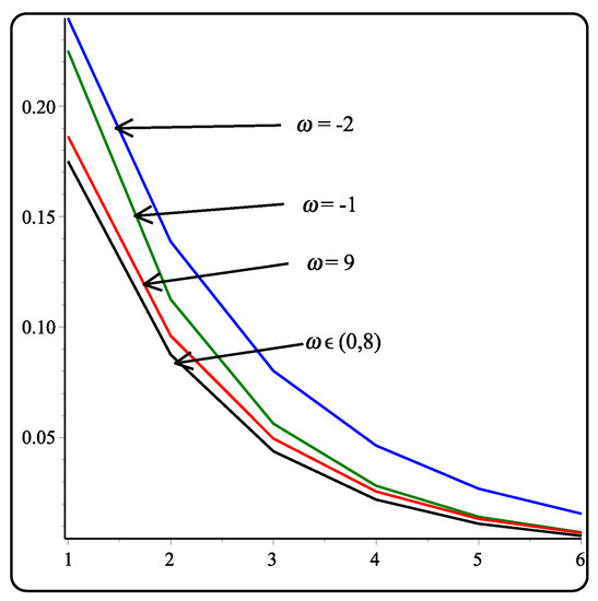
Figure 1. Error bounds of binary scheme (Equation (3)).

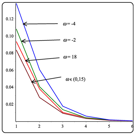
Figure 2. Error bounds of ternary scheme (Equation (12)).

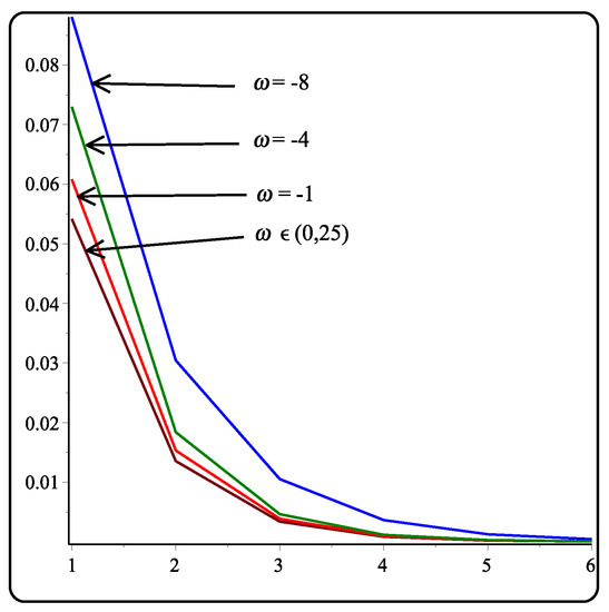
Figure 3. Error bounds of Quaternary scheme (Equation (18)).

4.2. Continuity

This section describes the effects of parameters for the schemes in Equations (3), (12), and (18). The order of continuity and effects of parameters $\omega$ of the schemes are shown in Table 4, Table 5 and Table 6, respectively. This can easily be found over the parametric intervals using the approach of Hassan [8].

Table 4. Continuity order of binary scheme (Equation (3)).

Scheme	Parameter	Continuity	Scheme	Parameter	Continuity
Binary	$-9<\omega <\frac{72}{5}$	$C^0$	Binary	$-2<\omega <6$	$C^4$
Binary	$-9<\omega <\frac{72}{5}$	$C^1$	Binary	$-2<\omega <6$	$C^5$
Binary	$-6<\omega <10$	$C^2$	Binary	$0<\omega <2$	$C^6$
Binary	$-6<\omega <10$	$C^3$	Binary	$\omega =1$	$C^7$

Table 5. Continuity order of ternary scheme (Equation (12)).

Scheme	Parameter	Continuity
Ternary	$\frac{-2929}{9}<\omega <\frac{356}{9}$	$C^0$
Ternary	$-23<\omega <31$	$C^1$
Ternary	$-14<\omega <22$	$C^2$
Ternary	$-8<\omega <16$	$C^3$
Ternary	$-4<\omega <12$	$C^4$
Ternary	$\omega =\frac{4}{3}$	$C^5$

Table 6. Continuity order of Quaternary scheme (Equation (18)).

Scheme	Parameter	Continuity
Quaternary	$\frac{-3775}{51}<\omega <\frac{4415}{51}$	$C^0$
Quaternary	$-57<\omega <71$	$C^1$
Quaternary	$-26<\omega <38$	$C^2$
Quaternary	$-24<\omega <36$	$C^3$
Quaternary	$-4<\omega <8$	$C^4$
Quaternary	$\omega =2$	$C^5$

4.3. Shapes of Limit Curves

The parametric effect and continuity of the limit curve of the schemes are shown in Figure 4, Figure 5 and Figure 6, respectively. These figures illustrate the role of free parameters when 5-point binary, ternary, and quaternary approximating schemes are applied on discrete data point. One can see the looseness/tightness of the limit curves in Figure 4, Figure 5 and Figure 6 when the parameter values change.

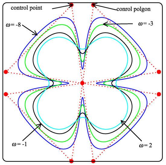
Figure 4. Parameter effects on the limit curves with initial polygon of binary scheme.

Figure 5. Parameter effects on the limit curves with initial polygon of ternary scheme.

Figure 6. Parameter effect on the limit curves with initial polygon of quaternary scheme.

5. Conclusions

In this work, we introduce the family of 5-point schemes which depict the representation of a wide variety of shapes with high smoothness (continuity) and less computational cost (processing time). These properties are useful in computer aided geometric design and geometric modeling. We apply Laurent polynomial to analyze our schemes. The shape parameter $\omega$ makes it able to provide different results along with its applications.

References

- De Rham, G. Un peu de mathématiques à propos d’une courbe plane. Elem. Math. 1947, 2, 73–76. [Google Scholar]
- Chaikin, G.M. An algorithm for high-speed curve generation. Comput. Gr. Imag. Process. 1974, 3, 346–349. [Google Scholar] [CrossRef]
- Doo, D.; Sabin, M. Behaviour of recursive division surfaces near extraordinary points. Comput. Aided Des. 1978, 10, 356–360. [Google Scholar] [CrossRef]
- Catmull, E.; Clark, J. Recursively generated B-spline surfaces on arbitrary topological meshes. Comput. Aided Des. 1978, 10, 350–355. [Google Scholar] [CrossRef]
- Deslauriers, G.; Dubuc, S. Symmetric iterative interpolation processes. In Constructive Approximation; DeVore, R.A., Saff, E.B., Eds.; Springer: Boston, MA, USA, 1989; pp. 49–68. [Google Scholar]
- Dyn, N.; Levine, D.; Gregory, J.A. A butterfly subdivision scheme for surface interpolation with tension control. ACM Trans. Gr. 1990, 9, 160–169. [Google Scholar] [CrossRef]
- Cai, Z. Convergence, error estimation and some properties of four-point interpolation subdivision scheme. Comput. Aided Geom. Des. 1995, 12, 459–468. [Google Scholar]
- Hassan, M.F.; Ivrissimitzis, I.P.; Dodgson, N.A.; Sabin, M.A. An interpolating 4-point C2 ternary stationary subdivision scheme. Comput. Aided Geom. Des. 2002, 19, 1–18. [Google Scholar] [CrossRef]
- Hassan, M.; Dodgson, N.A. Ternary and Three-point Univariate Subdivision Schemes; No. UCAM-CL-TR-520; Cambridge Computer Laboratory: Cambridge, UK, September 2001. [Google Scholar]
- Mustafa, G.; Liu, X. A subdivision scheme for volumetric models. Appl. Math. J. Chin. Univ. 2005, 20, 213–224. [Google Scholar] [CrossRef]
- Siddiqi, S.S.; Ahmad, N. A C6 approximating subdivision scheme. Appl. Math. Lett. 2008, 21, 722–728. [Google Scholar] [CrossRef]
- Hormann, K.; Sabin, M.A. A family of subdivision schemes with cubic precision. Comput. Aided Geom. Des. 2008, 25, 41–52. [Google Scholar] [CrossRef]
- Faheem, K.; Mustafa, G. Ternary six-point interpolating subdivision scheme. Lobachevskii J. Math. 2008, 29, 153–163. [Google Scholar] [CrossRef]
- Mustafa, G.; Khan, F. A new 4-point quaternary approximating subdivision scheme. Abstr. Appl. Anal. 2009, 2009. [Google Scholar] [CrossRef]
- Mustafa, G.; Khan, F.; Ghaffar, A. The m-point approximating subdivision scheme. Lobachevskii J. Math. 2009, 30, 138–145. [Google Scholar] [CrossRef]
- Siddiqi, S.S.; Rehan, K. Modified form of binary and ternary 3-point subdivision schemes. Appl. Math. Comput. 2010, 216, 970–982. [Google Scholar] [CrossRef]
- Mustafa, G.; Ghaffar, A.; Khan, F. The odd-point ternary approximating schemes. Am. J. Comput. Math. 2011, 1, 111–118. [Google Scholar] [CrossRef]
- Ghaffar, A.; Mustafa, G.; Qin, K. Unification and application of 3-point approximating subdivision schemes of varying arity. Open J. Appl. Sci. 2012, 2, 48–52. [Google Scholar] [CrossRef]
- Ghaffar, A.; Mustafa, G.; Qin, K. The 4-point 3-ary approximating subdivision scheme. Open J. Appl. Sci. 2013, 3, 106–111. [Google Scholar] [CrossRef]
- Mustafa, G.; Ghaffar, A.; Aslam, M. A subdivision-regularization framework for preventing over fitting of data by a model. AAM 2013, 8, 178–190. [Google Scholar]
- Mustafa, G.; Ashraf, P.; Deng, J. Generalized and unified families of interpolating subdivision schemes. Numer. Math. Theory Method. Appl. 2014, 7, 193–213. [Google Scholar] [CrossRef]
- Siddiqi, S.S.; Younis, M. The Quaternary Interpolating Scheme for Geometric Design. Int. Sch. Res. Not. 2013, 2013. [Google Scholar] [CrossRef]
- Rehan, K.; Siddiqi, S.S. A Family of Ternary Subdivision Schemes for Curves. Appl. Math. Comput. 2015, 270, 114–123. [Google Scholar] [CrossRef]
- Rehan, K.; Sabri, M.A. A combined ternary 4-point subdivision scheme. Appl. Math. Comput. 2016, 276, 278–283. [Google Scholar] [CrossRef]
- Ashraf, P.; Sabir, M.; Ghaffar, A.; Nisar, K.S.; Khan, I. Shape-Preservation of Ternary Four-point Interpolating Non-stationary Subdivision Scheme. Front. Phys. 2020, 7. [Google Scholar] [CrossRef]
- Ghaffar, A.; Ullah, Z.; Bari, M.; Nisar, K.S.; Al-Qurashi, M.M.; Baleanu, D. A new class of 2m-point binary non-stationary subdivision schemes. Adv. Differ. Equ. 2019, 2019, 325. [Google Scholar] [CrossRef]
- Ghaffar, A.; Ullah, Z.; Bari, M.; Nisar, K.S.; Baleanu, D. Family of odd point non-stationary subdivision schemes and their applications. Adv. Differ. Equ. 2019, 2019, 1–20. [Google Scholar] [CrossRef]
- Ghaffar, A.; Bari, M.; Ullah, Z.; Iqbal, M.; Nisar, K.S.; Baleanu, D. A New Class of 2q-Point Nonstationary Subdivision Schemes and Their Applications. Mathematics 2019, 7, 639. [Google Scholar] [CrossRef]
- Ghaffar, A.; Iqbal, M.; Bari, M.; Muhammad Hussain, S.; Manzoor, R.; Sooppy Nisar, K.; Baleanu, D. Construction and Application of Nine-Tic B-Spline Tensor Product SS. Mathematics 2019, 7, 675. [Google Scholar] [CrossRef]
- Dyn, N.; Iske, A.; Quak, E.; Floater, M.S. Tutorials on Multiresolution in Geometric Modelling, Summer School Lecture Notes Series: Mathematics and Visualization; Springer Science & Business Media: Berlin, Germany, 2002. [Google Scholar]
- Mustafa, G.; Hashmi, M.S. Subdivision depth computation for n-ary subdivision curves/surfaces. Vis. Comput. 2010, 26, 841–851. [Google Scholar] [CrossRef]
© 2020 by the authors. Licensee MDPI, Basel, Switzerland. This article is an open access article distributed under the terms and conditions of the Creative Commons Attribution (CC BY) license (http://creativecommons.org/licenses/by/4.0/).