Abstract
Shape preservation has been the heart of subdivision schemes (SSs) almost from its origin, and several analyses of SSs have been established. Shape preservation properties are commonly used in SSs and various ways have been discovered to connect smooth curves/surfaces generated by SSs to applied geometry. With an eye on connecting the link between SSs and applied geometry, this paper analyzes the geometric properties of a ternary four-point rational interpolating subdivision scheme. These geometric properties include monotonicity-preservation, convexity-preservation, and curvature of the limit curve. Necessary conditions are derived on parameter and initial control points to ensure monotonicity and convexity preservation of the limit curve of the scheme. Furthermore, we analyze the curvature of the limit curve of the scheme for various choices of the parameter. To support our findings, we also present some examples and their graphical representation.
Keywords:
Monotonicity-preservation; convexity-preservation; curvature; rational interpolating; subdivision schemes MSC:
65D17; 65D05; 65U07
1. Introduction
Shape preservation has great practical importance in the designing of curves/surfaces tailored to industrial design (e.g., related to car, aeroplane or ship modelling where convexity is imposed by technical and physical conditions as well as by aesthetic requirements). These properties are used in the design of curves or surfaces to predict or control their ‘shape’ by the shape of the control points, that is, the vertices of a given polygonal arc or polyhedral surface. Efficient methods to construct shape-preserving approximations starting from an initial data sequence are shape-preserving subdivision schemes, that is, schemes that preserve the shape for instance, the monotonicity or the convexity of the control points. In the past years, the shape preservation of limit curves has been a reliable topic in research. The main desirable properties for the implementation of smooth curves are monotonicity and convexity preservation.
Yadshalom [1] proposed a class of subdivision scheme having finite support of curve designing which preserved monotonicity. Carnicer and Dahmen [2] examined a characterization of strict convexity preserving subdivision schemes (SS). Dyn et al. [3] introduced interpolatory 4-point SS for curve designing, which preserved convexity. Kuijt and Damme [4] examined interpolating SS on shape preservation for non-uniform data. They also presented sufficient conditions for convexity preservation. Cai [5] introduced four-point ternary interpolating SS which preserved convexity and having a limit curve. A convexity preserving binary six-point linear approximating SS was presented by Hao et al. [6]. Mustafa et al. [7] introduced n-ary interpolating SS in which convexity preservation of the scheme was also examined. Floater et al. [8] offered monotonicity preservation of input data having conditions that assure differentiability to the limit function of the SS.
The shape-preserving property of ternary SS with the bell-shaped mask was examined by Pitolli [9]. A six-point interpolating ternary SS was presented by Mustafa and Ashraf [10], in which smoothness and differentiability of limit curves were discussed. Further, Siddiqi and Noreen [11] analyzed convexity preservation of six-point ternary interpolating SS. Akram et al. [12] proposed binary 4-point interpolating non-stationary scheme which preserved positivity, monotonicity, and convexity. Wang and Li [13] offered a five-point binary scheme that preserved convexity.
Mustafa and Bashir [14] dealt with the univariate scheme and its non-tensor product generalization of bivariate SS. The proposed schemes preserved the monotonicity of initial data. Novara and Romani [15] gave the conditions that the free parameter of the interpolating 5-point ternary SS and the vertices of a strictly convex initial polygon needs to ensure the convexity preservation of the limit curve. Asghar et al. [16] examined SS on probability distribution which has high continuity. The family of SS preserved convexity. A class of non-stationary -point binary scheme was presented by Ghaffar et al. [17]. They analyzed curvature and torsion of the limit curves of the proposed schemes. Zulkifli et al. [18] discussed the application of new rational bi-cubic Ball function with six parameters in image interpolation, especially for the gray scale image. For more recent work on SS one may refer to References [19,20,21,22,23].
A SS is said to be rational when the coefficients of the scheme are rational numbers. A ternary four-point rational scheme (-scheme) was presented by Peng [24].
The -scheme plots a polygon to define polygon by connecting the resultant subdivision rule and having set of control points at level .
such that
where the set of non-zero coefficients is called the mask of the scheme and u is shape parameter. The necessary condition for the convergence of SS is
Using Equation (3), it is evident that (4) is convergent. Peng et al. [24] proved that the -scheme generates limit curves when . They also analyzed the fractal behaviour of the scheme.
This motivated us to present the analysis of the geometric properties of the -continuous ternary scheme which is capable of producing fractal curves. In order to show the performance of the ternary scheme, we analyze the geometric properties such as monotonicity-preservation, convexity-preservation and curvature of the limit curve. Moreover, the limit curves with specific value of shape control parameter u are depicted by significant application of derived conditions on the initial data. The rest of the paper is organized as follows: In Section 2, we present geometric properties of the -scheme. Numerical examples and conclusions are discussed in Section 3.
2. Geometric Properties of the -Scheme
In this section, we present the geometric properties of the limit curves generated by the -scheme. These geometric properties consist of monotonicity-preservation, convexity preservation and curvature of the limit curves of the geometric properties.
2.1. Monotonicity Preservation
Here we discuss the monotonicity preserving property of the -scheme. For monotonicity preservation, we consider monotone control polygon since the limiting curve generated by the -scheme preserves the monotonicity of initial data. The monotonicity preservation of the -scheme can be obtained by applying the first order divided difference (DD) as . Thus the first order DD-scheme of (4) can be written as
For convenience, we introduce a new parameter in terms of u. For this let , so the value of u in terms of , can be written as:
Theorem 1.
Given a set of initial control points which are monotonically increasing, such that . Let
Furthermore, the parameter ω satisfies . If , is defined by the -scheme (4), then
Thus, the -scheme preserves monotonicity for initial monotone data.
Proof.
To prove (8), we use mathematical induction.
By assumption it is clear that (8) holds for . Suppose that (8) holds for , next we verify that it also holds for .
In order to show that (8) is true for , we first prove that .
As
For convenience put , we get
Thus
Now consider
Since , so and , then we have
Thus
Now consider
Therefore
Since
Now consider
By Equation (9), the denominator of the above equation is greater and equal to zero, and the numerator A satisfies
Therefore, .
Further we have
Now consider
By Equation (10), the denominator of the above equation is greater and equal to zero, and the numerator B satisfies
Thus
Similarly
So
By Equation (11), the denominator of the above equation is greater and equal to zero, and the numerator C satisfies
Therefore .
By following same steps, we can also prove , and . Therefore, and by induction, we have , , .
This completes the proof. □
2.2. Convexity Preservation
Now we discuss the convexity preservation of the -scheme. For convexity preservation, we consider convex control polygon so the limiting curve generated by the -scheme preserves convexity of initial data. The convexity preservation of the -scheme can be obtained by applying second order DD as .
For convenience, we introduce a new parameter instead of u. For this let and , so the value of u in terms of can be expressed as
Theorem 2.
Given a set of initial control points which are convex, such that , denote , . Furthermore, the parameter σ satisfies . If , is defined by the -scheme (4), then
Thus, the -scheme preserves convexity for initial convex data.
Proof.
To prove (15), we use mathematical induction.
By assumption it is clear that (15) holds for . Assume that (15) also holds for , next we verify that it also holds for .
In order to show that (15) is true for , we first show that .
As
For convenience put , we get
Thus
Now consider
Thus
Now consider
Therefore
Consider
Further, we have
By Equation (16), the denominator of the above equation is greater and equal to zero, and the numerator D satisfies
Therefore, .
Similarly
Since
By Equation (17), the denominator of the above equation is greater than and equal to zero, and the numerator E satisfies
Thus, .
Also
it follows
By Equation (18), the denominator of the above equation is greater than and equal to zero, and the numerator F satisfies
Therefore, .
By following same steps we can also prove , and . Therefore, , and by induction, we have , .
This completes the proof. □
2.3. Curvature
In mathematics, curvature is any of several strongly related concepts in geometry. Intuitively, the curvature is the amount by which a curve deviates from being a straight line, or a surface deviates from being a plane. Curvature is very important property not only in continuous geometry but also in network applications; see Reference [25].
The quality of SS can be measured quantitatively by finding curvature, as functions of cumulative chord length. We use the method described in Reference [17] to determine the curvature and numerical simulations are provided to illustrate the effects of various choices of shape parameter on curvature. Since the -scheme is parametric, it is obvious to see the results for various choices of the parameter u. Here we measure the curvature of limit curves of the -scheme for various choices of u. In Figure 1 and Figure 2, we consider a control polygon of a circle. The shape of the circle is obtained by applying an -scheme five times on this initial control polygon for various choices of parameter u. These limit curves are shown in Figure 1a,b and Figure 2a,b, while their corresponding curvatures are shown in Figure 1c,d and Figure 2c,d. In Figure 3 and Figure 4, we consider a star-shaped closed control polygon. The limit curves after applying the -scheme five times on this initial control polygon for various choices of parameter u is shown in Figure 3a,b and Figure 4a,b, while their corresponding curvatures are shown in Figure 1c,d and Figure 2c,d. In Figure 5 and Figure 6, we consider an open control polygon that presents the basic limit function of the scheme. The limit curves after applying the -scheme five times on this initial control polygon for various choices of parameter u is shown in Figure 5a,b and Figure 6a,b, while their corresponding curvatures are shown in Figure 5c,d and Figure 6c,d.
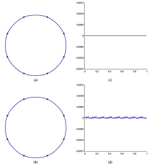
Figure 1.
Results for various choices of the parameter u are shown on the left together with their corresponding curvature on the right. From top to bottom: u = 0 and 0.0074. (a) Limit curve at ; (b) Limit curve at ; (c) Curvature plot of (a); (d) Curvature plot of (b).
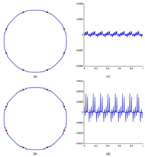
Figure 2.
Results for various choices of the parameter u are shown on the left together with their corresponding curvature on the right. From top to bottom: u = 0.0076 and 0.0077. (a) Limit curve at ; (b) Limit curve at ; (c) Curvature plot of (a); (d) Curvature plot of (b).
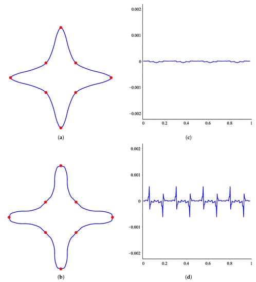
Figure 3.
Results for various choices of the parameter u are shown on the left together with their corresponding curvature on the right. From top to bottom: u = 0 and 0.0074. (a) Limit curve at ; (b) Limit curve at ; (c) Curvature plot of (a); (d) Curvature plot of (b).
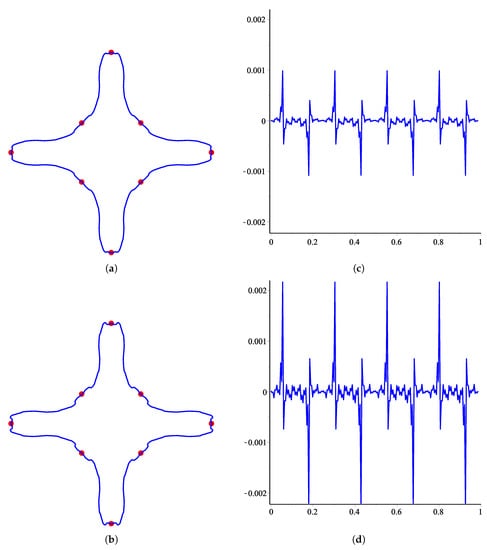
Figure 4.
Results for various choices of the parameter u are shown on the left together with their corresponding curvature on the right. From top to bottom: u = 0.0076 and 0.0077. (a) Limit curve at ; (b) Limit curve at ; (c) Curvature plot of (a); (d) Curvature plot of (b).
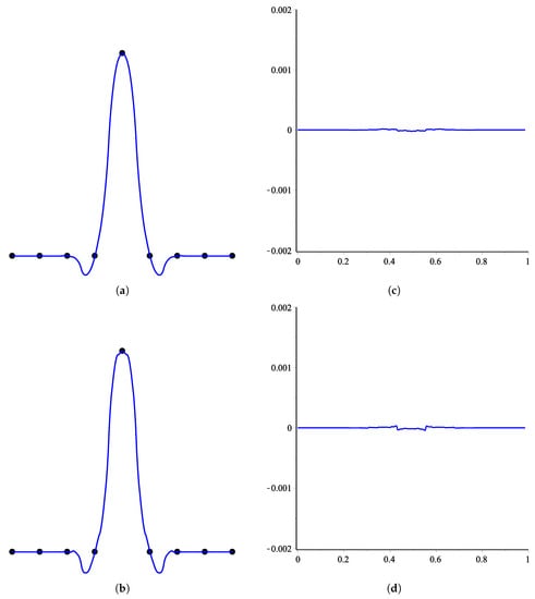
Figure 5.
Results for various choices of the parameter u are shown on the left together with their corresponding curvature on the right. From top to bottom: u = 0 and 0.0074. (a) Limit curve at ; (b) Limit curve at ; (c) Curvature plot of (a); (d) Curvature plot of (b).
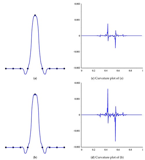
Figure 6.
Results for various choices of the parameter u are shown on the left together with their corresponding curvature on the right. From top to bottom: u = 0.0076 and 0.0077. (a) Limit curve at ; (b) Limit curve at ; (c) Curvature plot of (a); (d) Curvature plot of (b).
3. Numerical Examples and Conclusions
In this section, we present some numerical examples to show monotonicity and convexity preserving behaviour of the -scheme. At the end of the section, we discuss the conclusion of the work done so far.
3.1. Numerical Examples
We consider monotone data in Table 1 and Table 2. Figure 7 explains monotonicity preserving property of the -scheme. Figure 7a is generated by using monotone data as given in Table 1. In this figure, dotted lines show the initial set of values and the solid line represents the limit curve generated by the -scheme which is clearly monotonically increasing curve. Figure 7b is generated by using monotone data as given in Table 2. In this figure, dotted lines show the initial set of values and the solid line represents the limit curve generated by the -scheme, which is clearly monotonically increasing curve.

Table 1.
Monotone set of values.
Table 2.
Monotone set of values.
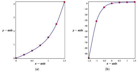
Figure 7.
The monotone curves generated by the -scheme (4). (a) Monotone curve at and (b) Monotone curve at .
We consider convex data in Table 3 and Table 4. Figure 8 explains convexity preserving property of the -scheme. Figure 8a is generated by using monotone data as given in Table 3. In this figure, dotted lines show the initial set of values and the solid line represents the limit curve generated by the -scheme which is clearly monotonically increasing curve. Figure 8b is generated by using monotone data as given in Table 4. In this figure, dotted lines show the initial set of values and the solid line represents the limit curve generated by the -scheme which is clearly monotonically increasing curve.
Table 3.
Convex set of values.
Table 4.
Convex set of values.
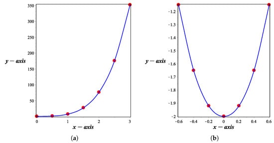
Figure 8.
The convex curves generated by the -scheme (4). (a) Convex curve at and (b) Convex curve at .
3.2. Conclusions
In this paper, we have presented geometrical properties of the -scheme, which improves on the scheme in various ways that meet different requirements. These geometric properties demonstrate that the shape-preservation of the limit curve is a useful mechanism for modifying the -scheme. We have shown that by taking initial control data monotone and convex, the limit curves generated by the -scheme are also monotone and convex. As observed, the -scheme for various choice of shape control parameter can be considered more universal. Several examples are given which support our findings. Finally, the same idea could be applied to bivariate surfaces. A useful extension of this work is to analyze shape preserving behaviour of SSs when scattered data is considered.
Author Contributions
Conceptualization, P.A. and A.G.; formal analysis, D.B., K.S.N. and S.A.; methodology, D.B., K.S.N. and S.A.; software, P.A., B.N., A.G. and M.A.A.K.; supervision, D.B.; Writing—original draft, P.A., B.N. and A.G.; Writing—review & editing, K.S.N., D.B. and S.A. All authors have read and agreed to the published version of the manuscript.
Funding
This research received no external funding.
Conflicts of Interest
The authors declare no conflict of interest.
References
- Yadshalom, I. Monotonicity preserving subdivision schemes. J. Approx. Theory 1993, 74, 41–58. [Google Scholar] [CrossRef]
- Carnicer, J.M.; Dahmen, W. Characterization of local strict convexity preserving interpolation methods by C1 functions. J. Approx. Theory 1994, 77, 2–30. [Google Scholar] [CrossRef][Green Version]
- Dyn, N.; Kuijt, F.; Levin, D.; Van Damme, R. Convexity preservation of the four-point interpolatory subdivision scheme. Comput. Aided Geom. Des. 1999, 16, 789–792. [Google Scholar] [CrossRef]
- Kuijt, F.; Van Damme, R. Shape preserving interpolatory subdivision schemes for non-uniform data. J. Approx. Theory 2002, 114, 1–32. [Google Scholar] [CrossRef]
- Cai, Z. Convexity preservation of the interpolating four-point C2 ternary stationary subdivision scheme. Comput. Aided Geom. Des. 2009, 26, 560–565. [Google Scholar] [CrossRef]
- Hao, Y.X.; Wang, R.H.; Li, C.J. Analysis of a 6-point binary subdivision scheme. Appl. Math. Comput. 2011, 218, 3209–3216. [Google Scholar] [CrossRef]
- Mustafa, G.; Deng, J.; Ashraf, P.; Rehman, N.A. The mask of odd points n-ary interpolating subdivision scheme. J. Appl. Math. 2012, 2012, 205863. [Google Scholar] [CrossRef]
- Floater, M.; Beccari, C.; Cashman, T.; Romani, L. A smoothness criterion for monotonicity preserving subdivision. Adv. Comput. Math. 2013, 39, 193–204. [Google Scholar] [CrossRef]
- Pitolli, F. Ternary shape-preserving subdivision schemes. Math. Comput. Simul. 2014, 106, 185–194. [Google Scholar] [CrossRef]
- Mustafa, G.; Ashraf, P. A new 6-point ternary interpolating subdivision scheme and its differentiability. J. Inf. Comput. Sci. 2010, 5, 199–210. [Google Scholar] [CrossRef]
- Siddiqi, S.S.; Noreen, T. Convexity preservation of six point C2 interpolating subdivision scheme. Appl. Math. Comput. 2015, 265, 936–944. [Google Scholar] [CrossRef]
- Akram, G.; Bibi, K.; Rehan, K.; Siddiqi, S.S. Shape preservation of 4-point interpolating non-stationary subdivision scheme. J. Comput. Appl. Math. 2017, 319, 480–492. [Google Scholar] [CrossRef]
- Wang, Y.; Li, Z. A family of convexity-preserving subdivision schemes. J. Math. Res. Appl. 2017, 37, 489–495. [Google Scholar]
- Mustafa, G.; Bashir, R. Univariate approximating schemes and their non-tensor product generalization. Open Math. 2018, 16, 1501–1518. [Google Scholar] [CrossRef]
- Novara, P.; Romani, L. On the interpolating 5-point ternary subdivision scheme: A revised proof of convexity-preservation and an application-oriented extension. Math. Comput. Simul. 2018, 147, 194–209. [Google Scholar] [CrossRef]
- Asghar, M.; Iqbal, M.J.; Mustafa, G. A family of high continuity subdivision schemes based on probability distribution. Mehran Univ. Res. J. Eng. Technol. 2019, 38, 389. [Google Scholar] [CrossRef]
- Ghaffar, A.; Ullah, Z.; Bari, M.; Nisar, K.S.; Al-Qurashi, M.M.; Baleanu, D. A new class of 2m-point binary non-stationary subdivision schemes. Adv. Differ. Equ. 2019, 2019, 325. [Google Scholar] [CrossRef]
- Zulkifli, N.A.B.; Karim, S.A.A.; Sarfraz, M.; Ghaffar, A.; Nisar, K.S. Image interpolation using a rational bi-cubic ball. Mathematics 2011, 7, 1045. [Google Scholar] [CrossRef]
- Ashraf, P.; Sabir, M.; Ghaffar, A.; Nisar, K.S.; Khan, I. Shape-preservation of ternary four-point interpolating non-stationary subdivision scheme. Front. Phys. 2020, 7, 241. [Google Scholar] [CrossRef]
- Ghaffar, A.; Ullah, Z.; Bari, M.; Nisar, K.S.; Baleanu, D. Family of odd point non-stationary subdivision schemes and their applications. Adv. Differ. Equ. 2019, 171, 1–20. [Google Scholar] [CrossRef]
- Ghaffar, A.; Bari, M.; Ullah, Z.; Iqbal, M.; Nisar, K.S.; Baleanu, D. A new class of 2q-point non-stationary subdivision schemes and their applications. Mathematics 2017, 7, 639. [Google Scholar] [CrossRef]
- Shahzad, A.; Khan, F.; Ghaffar, A.; Mustafa, G.; Nisar, K.S.; Baleanu, D. A novel numerical algorithm to estimate the subdivision depth of binary subdivision schemes. Symmetry 2020, 12, 66. [Google Scholar] [CrossRef]
- Zou, L.; Song, L.; Wang, X.; Chen, Y.; Zhang, C.; Tang, C. Bivariate thiele-like rational interpolation continued fractions with parameters based on virtual points. Mathematics 2020, 8, 71. [Google Scholar] [CrossRef]
- Peng, K.; Tan, J.; Li, Z.; Zhang, L. Fractal behavior of a ternary 4-point rational interpolation subdivision scheme. Math. Comput. Appl. 2018, 23, 65. [Google Scholar] [CrossRef]
- Shang, Y. Lack of Gromov-hyperbolicity in small-world networks. Cent. Eur. J. Math. 2011, 10, 1152–1158. [Google Scholar] [CrossRef]
© 2020 by the authors. Licensee MDPI, Basel, Switzerland. This article is an open access article distributed under the terms and conditions of the Creative Commons Attribution (CC BY) license (http://creativecommons.org/licenses/by/4.0/).