Abstract
Ecoacoustics is a recent ecological discipline focusing on the ecological role of sounds. Sounds from the geophysical, biological, and anthropic environment represent important cues used by animals to navigate, communicate, and transform unknown environments in well-known habitats. Sounds are utilized to evaluate relevant ecological parameters adopted as proxies for biodiversity, environmental health, and human wellbeing assessment due to the availability of autonomous audio recorders and of quantitative metrics. Ecoacoustics is an important ecological tool to establish an innovative biosemiotic narrative to ensure a strategic connection between nature and humanity, to help in-situ field and remote-sensing surveys, and to develop long-term monitoring programs. Acoustic entropy, acoustic richness, acoustic dissimilarity index, acoustic complexity indices (ACItf and ACIft and their evenness), normalized difference soundscape index, ecoacoustic event detection and identification routine, and their fractal structure are some of the most popular indices successfully applied in ecoacoustics. Ecoacoustics offers great opportunities to investigate ecological complexity across a full range of operational scales (from individual species to landscapes), but requires an implementation of its foundations and of quantitative metrics to ameliorate its competency on physical, biological, and anthropic sonic contexts.
1. Introduction
A tremendous acceleration of biodiversity decline has been recently denounced by several governmental and non-governmental organizations on scientific and popular media in a continuative ‘war bulletin.’ A growing scientific debate on priorities and remediation strategies to preserve ecosystem services and human wellbeing is still open and in progress [1]. The growing intrusion of humans in the environment has produced forest fragmentation [2], cropland expansion, food insecurity [3,4], biomass stock reduction [5], water and air pollution [6], impervious surface increase [7], and global land and climate change [8,9], and associated with the reduction of ecosystem services [10] to list some of the common widespread effects.
Today, the use of satellites to monitor terrestrial and aquatic systems at the planetary scale is becoming a routine practice [11], and this extensive use of remote sensing associated with big data analysis has increased the amount of environmental knowledge available to civil society, stakeholders, and policymakers. However, civil society must control numerous threats at multiple scales and continuously provide new scientific approaches to convert the flux of environmental data into useful suggestions for more efficient management of natural resources [12]. For instance, more accurate detection and protection of the hot spots of biodiversity [13,14], or trading biodiversity, which results in an important strategy to reduce the effect of pests on food production and security [15], which are some of the new strategies to drive human development toward a more sustainable future.
Despite the massive diffusion of satellites to remotely survey environments, several aspects of ecological dynamics remain unexplored. For instance, although odors and sounds are two components of the environment relatively known at the level of individual species’ sensory and behavior, up to now, they have been insufficiently used to monitor ecological dynamics at a large scale. In particular, sounds have the potentiality to play a primary role to describe the composition, diversity, and dynamics of (acoustic) communities [16], and to assess the distance of ecosystems from healthy conditions [17,18].
The study of environmental sound captures a greater number of details when compared to visual information alone [19] and offers several advantages. In particular, acoustic surveys using autonomous audio recording devices have a negligible effect on the environment, provide continuous observations, and reduce any bias introduced by human presence when using traditional invasive surveys (e.g., netting, trapping, and marking). Furthermore, with the application of new powerful metrics, a great amount of acoustic data can be processed, and the patterns and dynamics of the acoustic environment can be described in detail.
This paper aims to present environmental sound as a subject of investigation according to an ecological perspective. In particular, the fundaments of environmental acoustics; relevance of quantitative analysis of sound to environmental monitoring schemes, to nature conservation, and to human wellbeing improvement; and the most popular and efficient metrics used in the quantitative approach to sound investigation are described.
2. Environmental Sound, General Characters, and Importance
Nature is not silent. Physical surficial attrition and soniferous species create a great number of sounds belonging to different frequencies, intensities, and duration that can be interpreted differently by animals according to specific functions that are activated at the moment [20]. Sounds propagate in the air at 331 m/s at 0°, and propagate five times faster (1484 m/s) in water with high variability. This variability in sound transmission depends on the physical characters of the medium (density, temperature, salinity, shape of the surfaces, etc.) and on the position of emitters and receivers.
Sounds can be classified according to the geophysical, biological, and anthropic source. Waterfalls, marine waves, winds, thunderstorm, lightning, and volcanoes are examples of geophysical sounds (geophonies). The biological sounds (biophonies) are the result of active vocalizations of soniferous species obtained by different organs (e.g., vocal chords in mammals, syrinx in birds, vocal sacs in frogs, tymbals in cicadas, etc.). The anthropogenic sounds (technophonies) are the result of synthetic technologies/activities like machineries and vehicles, music, explosions, urban areas, and industries.
In both terrestrial and aquatic systems, sounds contain important information that is extensively used by a great number of animals in intra- and inter-species communication creating a complex network of emitters and receivers [21]. Sensitivity to sound extends to the plant kingdom [22], and sound-mediated relationships exist between kingdoms. For example, Schöner et al. [23] demonstrated the acoustically mediated co-evolution of some species of plants and bats.
Sounds are actively used in animal navigation [24] and to transform an unknown environment into a friendly collection of reference points [25]. For instance, the sound of sea waves crashing against a reef is used by pelagic larvae of reef fishes and decapod crustaceans to orient their migration toward reef refuges [26,27]. Sounds at high frequency emitted by whales, dolphins, and bats are used as sonar to locate food and obstacles [28,29]. Sound is a primary vehicle used by soniferous species to provide information on individual fitness and can be considered an honest signal [30,31]. Biological sounds have plastic characters that can be modified by learning or culturally transmitted adaptive processes [32,33,34].
From a human perspective, sound has further characteristics; it is considered a source of pleasure, contributes to creating a sense of place, and maintains and reinforces cultural heritage and wellbeing [35,36]. Sound, when too intense and/or continuous, like urban technophonies, is considered a source of noise and may cause masking effects on other (biological) sounds, producing an interruption of the communication networks with consequences on the physiology of sensitive species [37,38]. In terrestrial habitats, noise produced by the transit of snowmobiles has been documented to modify the physiology of the elk population in Yellowstone National Park [39]. In marine systems, the coral reef fish communities are negatively affected by the passage of boats [40]. In marine habitats, the noise level may be considered a real source of diffuse pollution with severe consequences on life [41], and in the next decades, it is expected to increase from commercial ships [42].
Noise can produce change in the habits of animal communities. For example, birds living around airports have been observed to anticipate the dawn chorus before the beginning of the morning take-off and airplane landing [43,44]. The adaptation to urban noise may reduce the individual fitness, as observed in white-crowed sparrows (Zonotrichia leucophrys) in the San Francisco area [45]. Noise may also be a cause of environmental avoidance for noise-sensitive species, like nest predators among birds [46]. Consequences of urban noise on animals are not well understood and remain a fertile ground for future research and acoustic monitoring, both urgently requested at the local and global scales [47]. In addition, the World Health Organization has considered noise as a major threat to human wellbeing [48]. For instance, a persistent urban noise exposition in human populations may be a relevant cause of cardiovascular diseases [49].
3. Ecoacoustics as a New Scientific Discipline
The interest in the influence of the physical and biological structure of the environment on sound diffusion [50,51,52,53] and the acoustic character of the environment [54,55,56,57] has a long history, with research dating back at least 50–60 years. However, the recent seminal papers of Pijanowski et al. [58,59], who focused on the role of the soundscape in the acoustic environment in which soniferous and non-soniferous species are embedded, facilitated the emergence of ecoacoustics as a novel independent discipline founded in Paris just a few years later (2014) during a scientific meeting on environmental acoustics [60,61,62].
Two facts contributed to the development of ecoacoustics: The availability of autonomous audio recorders and the use of powerful metrics to analyze acoustic data quantitatively. The possibility to deploy several recorders that are programmable according a flexible time table allows collecting contemporary acoustic information in different locations at different temporal resolutions [63]. This technology makes long-term acoustic exploration possible for hostile or remote environments, such as some tropical forests or deep seas, where other sensing tools like visual surveys are impossible or ineffective.
An interesting epistemological lexicon has been created since ecoacoustics was established as an independent scientific discipline. The sound can be interpreted by distinguishing between at least three functional scales: Soniferous species, acoustic communities, and soundscape. At the soniferous species level, the functions activated by sounds have influence on the following:
- species distribution across the habitat,
- daily and seasonal changes of individual acoustic activity,
- intra- and inter-specific interactions,
- acoustic variation of individual species and populations across different landscape/waterscape configurations,
- acoustic biogeography (dialects) of species and populations, and
- seasonal fluctuations and density of populations.
The acoustic community is an important model recently developed inside the ecoacoustic epistemology. An acoustic community is the ensemble of biophonies that result from the temporary combination of individual inter-specific sounds [64,65,66] and is characterized by a temporal variation in species composition according to hourly, daily, and seasonal species turnover. Human intrusion and climate change may produce significant changes in acoustic composition and dynamics in acoustic communities.
The soundscape is the character of the entire set of sounds of geophysical, biological, and technological origin that emerge from the environment. Geographical and ecological gradients may affect the acoustic signatures of a soundscape [67]. Sense of place and other human-related psychological feelings are associated with the quality and unity of soundscapes. Human intrusion, management strategies, and climate change are important factors that can influence soundscapes and their acoustic signature. Preserving a soundscape means to protect biodiversity and human cultural heritage, and it passes through a complex integration of knowledge and managing rules [68].
4. Quantitative Methods in Ecoacoustics
4.1. Hardware
The quantitative methods proposed by ecoacoustics have been strongly influenced by the recent availability of digital autonomous audio recorders characterized by a long charge and flexible programmability. Wildlife acoustics (USA; https://www.wildlifeacoustics.com), Lunilettronik (ITL; http://www.lunilettronik.it), and Frontier Labs (AU; http://www.frontierlabs.com.au) are the main producers of professional terrestrial and aquatic recorders for bioacoustic and ecoacoustic investigations. The use of low-cost recorders has been recently proposed [69] and new devices (e.g., Audio Moth (https://www.openacpisticdevices.info/)) tested [70] as a further solution to deploy recorders in unsafe places where human vandalism or animal damage discourage the use of more expensive devices.
4.2. Ecoacoustic Metrics
A second relevant point that favors the diffusion of the ecoacoustic approach is represented by the possibility to analyze acoustic files and convert them from a temporal domain to a frequency domain (e.g., after Fourier transforms). Several indices working on a matrix of frequency band intensity have been provided in recent years (for a review, see Sueur et al. [71]) with successful attempts to use such indices to estimate avian species diversity and assess biodiversity in general [16,72]. These indices can be distinguished in the following:
- intensity indices that measure sound amplitude,
- complexity indices that measure the level of complexity (time, frequency, and/or amplitude), and
- soundscape indices that investigate the importance of geophonies, biophonies, and technophonies.
Ecoacoustic metrics can be used as proxies for ecosystem functioning across spatial and temporal scales, but are generally not adapted to carry out direct species identification.
4.2.1. Intensity Indices
The intensity indices are based on the measurement of sound level (i.e., LCpeak, LAeq) and require expensive instruments to measure the amount of sonic energy. These indices are rarely utilized in ecoacoustic investigations.
4.2.2. Complexity Indices
Complexity indices assume that acoustic complexity increases with the number of singing individuals and species, representing a good proxy of animal phenology and diversity. The most popular indices are described below. A comparison between ecoacoustic metrics can be found in the works by Xie et al. (2017) [73], Turner et al. (2018) [74], and Rice et al. (2017) [75].
Acoustic entropy [16] is composed of two sub-indices: temporal entropy Ht and spectral entropy Hf.
These two indices are calculated by applying the Shannon equation:
where n is the length of the signal in the number of digitized points, A(t) is the probability mass function of the amplitude envelope, and S(f) is the probability mass function of the mean spectrum, applying a short-time Fourier transform (STFT).
Acoustic richness (AR) [76] results from the following equation:
where M is the median (A(t))*2(1−depth), where 0 ≤ M ≤ 1, and A(t) is the amplitude envelope, where the depth is the signal digitization depth.
The acoustic dissimilarity index [16] (D = Dt*Df) estimates the ß diversity between two acoustic communities. This index is composed by two sub-indices: temporal dissimilarity Dt and spectral dissimilarity Df, where 0 ≤ D ≤ 1:
where A1(t) and A2(t) are the probability mass functions of the amplitude envelope of the two acoustic files under comparison, and S1(f) and S2(f) are the probability mass functions of the mean spectrum.
The acoustic complexity index (ACI) was proposed in 2008 by Farina and Morri [77] and represents one of the most utilized ecoacoustic metrics since the first edition in 2011 [78]. The ACI measures the amount of (syntactic) information of a matrix of sound amplitude obtained after the application of a fast Fourier transform (FFT) on an acoustic file. The ACI is based on a simple algorithm that calculates the absolute difference between two adjacent values of acoustic amplitude [79]. This difference is considered acoustic (syntactic) information. As more differences occur and more information is contained within the spectrogram, the acoustic environment should be more complex and variable. Generally, a high number of soniferous species are associated with a high value of acoustic information. This index was successively distinguished in two sub-indices ACItf and ACIft [80], where ACItf is applied along the same frequency band and ACIft is calculated across all frequency bands at each temporal step selected for the analysis (e.g., one minute). The ACItf equation is as follows:
where ai,j is the amplitude of each pulse, t is the number of temporal steps in which a file is subdivided after FFT, f is the frequency bin, c is the number of clumps in the recording, and t/c is the number of elements composing a clumping. The clumping option allows the application of this equation to a selected number of aggregated temporal steps. The clumping option is not mandatory for ACItf. To compare two ACItf indices calculated on a different time interval, an average value must be used. The ACIft equation is as follows:
where ai,j is the amplitude of each pulse, t is the number of temporal intervals, and f is the frequency bins. Both Equations (6) and (7) are applied only in the presence of non-zero values of ai,j in each difference to reduce the edge effects.
From these two indices, an evenness measure has recently been obtained [80]. The evenness of ACI is an important metric because it measures how the acoustic information is distributed along frequency bands and time. In addition, ACItf evenness measures how the frequency classes are distributed at a specific time lag. Moreover, ACIft evenness measures how the spectral intensity is distributed along a specific time interval. Both the metrics are calculated according to equations by Levins [81] and Hurlbert [82]:
where pi is the importance of ACI in each frequency bin (ACItf) or in each temporal step t (ACIft) and the standardized measure is as follows:
This measure ranges from 0 to 1. For instance, if the window size for FFT is set at 512 frequency bins, the maximum evenness of ACItf evenness is 1/512, which means that all frequencies are distributed in the same way. A low value of ACItf evenness means that the information is concentrated in a few frequency bands. In addition, ACIft evenness is equal to 1 when the same amount of information exists at every temporal step. A low ACIft evenness indicates that the acoustic activity along a specific temporal step is concentrated only in one portion of the temporal window considered. Recently, ACItf evenness and ACIft evenness have been utilized to encode the ecoacoustic events using the ecoacoustic event detection and identification (EEDI) procedure [49,80].
Characteristics of ACItf and ACIft
The ACItf measure has been extensively validated at different temporal resolutions [83] in terrestrial [74,84] and aquatic systems [75,85,86,87,88]. Moreover, ACItf has been used to investigate animal phenology [89,90] and to estimate the effect of anthropogenic noise [91]. This index has also been demonstrated to be a good proxy of richness and diversity of the communities in forest areas [74,92] and marine and freshwater systems [93,94,95]. The graphic representation of ACItf depicts the acoustic signature. In a long-term temporal context, ACItf accurately describes changes in frequencies as a consequence of species turnover (Figure 1). A more recent index, ACIft has found a primary role in the development of the procedure to detect and identify ecoacoustic event metrics [96].
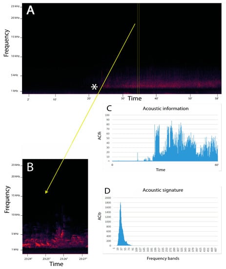
Figure 1.
Example of an application of the ACI metrics to an acoustic file in .wav format. In this case, the file has been recorded at Madonna dei Colli (Tuscany region, Italy) (44°12′29.84″ N, 10°03′33.08″ E; 228 m a.s.l.; slope exposition: East; mixed woodland) at 04:01 9 May 2018. The start of the dawn chorus (*) is indicated in the spectrogram (A) for one hour. (B) A magnification of a few seconds from 37′24″ to 37′27″ is represented in which the acoustic signature of the song of a blackbird (Turdus merula) is visible. (C) The distribution of the acoustic information (ACIft) along one hour (in y axis ACIft values, in x axis the time in minutes) (D) The acoustic signature (ACItf) along 487 frequency bins (where each bin is 46.87 Hz) (in y axis ACItf values, in x axis frequency bins). The first 15 bins have been excluded from the representation to eliminate instrumental noise.
4.2.3. Soundscape Indices
The soundscape indices consider the three components of the soundscape (geophonies, biophonies, and technophonies) and evaluate their importance and patterns created by their acoustic interactions. These indices are particularly relevant to evaluate the role of human intrusion in the environment and the sonic quality of a landscape in general.
Normalized Difference Soundscape Index
At the soundscape level, it is possible to investigate the proportion of technophonies and biophonies. An index called the Normalized Difference Soundscape Index (NDSI) was formulated by Kasten et al. [97]:
where α is the power spectral density (PSD) of sound in the range 1–2 kHz (technophonies) and β is the PSD of sound in the range 2–11 kHz (biophonies). This index ranges from −1 (all technophonies) to +1 (all biophonies). We must consider that some biophonies also include frequencies below 2 kHz. Geophonies often have broad spectral characteristics to be used in this typology of frequency index. To reduce the risk of biases, this index should be used on days without rain or wind.
Ecoacoustic Event Detection and Identification Routine (EEDI)
Every distinguished peculiarity in a spectrogram may be caused by natural or human induced causes (individual vocalizations (biophonies), geophysical or technophonic signals, or their combination). This peculiarity is defined according to a biosemiotic perspective of an ecoacoustic event [80]. Its extraction from a numerical matrix created by an FFT can be done automatically using the Ecoacoustic Event Detection and Identification routine (EEDI) [80]. This routine calculates the ACI metrics (ACIft, ACIft evenness, and ACItf evenness) and builds a code for every ecoacoustic event. These metrics, when combined, disclose emerging patterns inside an acoustic sequence that is a carrier of meaningful information for species to accomplish the needs required by every organism to stay alive with the best standard [80,96]. In detail, EEDI assigns a three-digit code to each ecoacoustic event, where the first number (from the left) is the value of ACIft, rescaled according 10 intervals (attributing zero to the first interval and nine to the last interval). The second (central) number is the value of ACIft evenness, and the third number is the value of ACItf evenness, both converted in 10 intervals as ACIft. The combination of these three numbers generates a maximum of 1000 codes (from 000 to 999).
According to a biosemiotic perspective, the temporal succession of ecoacoustic events can be considered “acoustic text” that can be detected and interpreted by individual species, assuming distinct species-specific meanings according the activated functions [80]. The ecoacoustic event model is based on the eco-field theory [98,99] that states that every function finalized to track a specific resource requires a distinct spatial configuration as a carrier of meaning. In this case, the acoustic eco-field is the result of the temporal and spatial arrangement of acoustic signals produced in the environment by geophonies, biophonies, and technophonies and perceived in a specific way by individual species. The number of ecoacoustic events detected along a temporal window is an indicator of the complexity of the acoustic community (when only biophonies are considered) or of soundscapes (when all sound sources are considered). The detection procedure is followed by an identification process that requires a training set of identified ecoacoustic events.
The EEDI procedure is a further step to improve the ecoacoustic methods moving out from the bioacoustic approach based on individual species identification to an ecoacoustic approach based on the identification of ecoacoustic events, disclosing properties of ecological functioning of habitats, ecosystems, or landscapes. Recently, how ecoacoustic events are strongly influenced by the temporal resolution at which the EEDI procedure is applied [100] has been demonstrated. To solve the uncertainty introduced by a subjective choice of a temporal resolution, a multiscale approach was proposed, and a fractal dimension calculated across this scale as an unbiased proxy of the acoustic complexity of a soundscape [100]. The fractal dimension is an independent measure of complexity and emerges as an important indicator of environmental conditions, where degraded environments should have a low fractal dimension and a healthy environment that is rich in soniferous species should have a high fractal dimension.
Finally, the multiscale approach of EEDI results is important from a biosemiotic point of view because it is possible to classify and assign specific meaning at each ecoacoustic event, transforming a frequency domain into a sequence of codes attributed to a species-specific functional role.
4.3. Passive Acoustic Monitoring for Environmental Assessment and Long-Term Passive Ecoacoustic Monitoring
Passive acoustic monitoring (PAM) is an ecosystem-based approach to assess long-term changes in community abundance, richness, and diversity primarily based on the aural identification of species [18,101,102]. This methodology is very popular in bioacoustic studies to monitor the abundance, distribution, and reproductive cycles of focus species (e.g., dolphins [103], koalas [104], whales [105], raptors [106], and snapping shrimp [107], or invasive species [108,109]) and landscape [110], to name some examples from numerous papers published in the last ten years.
When extended to an ecoacoustic approach (using appropriate metrics), PAM changes to passive ecoacoustic monitoring (PEM), which can also detect physical parameters from the environment, such as the rain regime [111], ocean weather [112], or temperature [113]. Empirical evidence of the efficiency of PEM has been accumulated on Mediterranean maqui [84], on temperate freshwater [85,114,115], and in the marine environment [116,117,118,119]. In particular, long-term monitoring of the soundscape is important to implement management and mitigation strategies [120]. Often, a combination of the aural species identification and the ecoacoustic metric offers a better description of acoustic communities and soundscapes.
5. Discussion and Conclusions
Ecoacoustics represents a new and promising ecological discipline from a theoretical and applied perspective, which can guarantee an efficient and updated environmental assessment and long-term monitoring. The quantitative approach of ecoacoustics provides important information about the ecological functioning of the environment across a broad range of spatial and temporal scales, integrating other ecological and biogeographic procedures. Sounds are indicators of many relevant ecological processes, such as biodiversity turnover, animal population, and community dynamics. For example, the sonic quality of a landscape may be utilized to select and preserve cultural heritage areas and to assess the human wellbeing level and availability of natural resources.
Sound is characterized by structured energy associated with a great amount of information. Sounds are energetic substrates on which is possible to test theories like the complexity theory and the cognitive theory of resources. The availability of several metrics to manipulate field data offers new possibilities of quantitative investigation of the environmental complexity.
The recording of sounds from different environments and geographic areas offers the possibility to make relevant comparisons between habitats and between different land-use policies, enlarging the investigation perspectives. For their inaccessibility, climatic hostility, and ecological complexity, some environments, such as deep oceans or tropical forests, represent a true challenge posed to traditional research. The placement of autonomous fully programmable acoustic recordings allows the collection of important information, especially over long periods, reducing the effect caused by other methodologies of field survey.
It is not a surprise that many issues in ecoacoustics remain underdeveloped. For example, the choice of the most effective index to capture typologies of biophonic sources remains unsatisfactory, as it is difficult to discriminate geophonies from technophonies and biophonies, limiting the acoustic patterns of an environment to favorable weather conditions [71]. Moreover, the choice of the most efficient temporal sampling schemes [18,84] requires further testing and empirical evidence before the adoption of a fully accepted standardization.
Some indices that are based on information theory and measure the acoustic entropy fail to reflect species richness and the abundance of individuals within each species and generally have a reduced capacity to describe the composition of the acoustic communities [89,121,122]. This requires other analytical methods that could be provided after more careful research for new mathematical tools [73,123]. However, the recent availability of software to calculate ecoacoustic indices using friendly languages like R appears relevant [124,125].
The ecoacoustic approach offers new possibilities to explore the biogeography ([126] and phenology of species [90,127]) that could be coupled with the effects of climatic change [18,87] and habitat degradation [128]. There are very few investigations on the relationship between soundscape and landscape [110], and this topic should be developed, coupling remote-sensing methodologies, and GIS with field recordings that are opportunely scaled.
In marine systems, ecoacoustics can be utilized to identify relatively pristine seas, to predict the effect of ocean industrialization before it occurs, and to suggest mitigation actions on the most vulnerable animal populations [41]. In urbanized areas, an ecoacoustic approach is considered to have an enormous potential to monitor urban biodiversity and ecosystem functioning [129]. The ecoacoustic approach allows the collection of a great amount of data for long periods of time, but this poses problems in terms of the effort to process such data, representing a challenging matter in ecoacoustic research. For example, urban areas (smart cities) are sources of acoustic big data due to the proliferation of mobile phone platforms. This poses problems for data reduction and analysis [130,131]. This fact forces us to concentrate on adapting methodologies to reduce the dimension of such big data and to improve their visualization [132].
Finally, ecoacoustics can reinforce the biosemiotic approach, translating acoustic cues into distinct signs that can be interpreted using a biosemiotic narrative. This narrative allows conjugating ecological issues with environmental humanities, concurring to reduce the dichotomy present, especially in Western cultures, between people and nature. Assigning a meaningful label to ecoacoustic events means to create a robust text that can describe the perceived reality of humans and animals and can help to adopt the best management choices. Robust encoding procedures are required for this, and due to operational multi-scaling, fractal mathematics could play a pre-eminent role in ecoacoustics in the immediate future.
Funding
This research received no external funding.
Conflicts of Interest
The author declares no conflict of interest.
References
- Masood, E. Battle over biodiversity. Nature 2018, 560, 423–425. [Google Scholar] [CrossRef]
- Ibisch, P.; Hoffmann, M.T.; Kreft, S.; Pe’er, G.; Kati, V.; Biber-Freudenberger, L.; DellaSala, D.A.; Vale, M.M.; Hobson, P.R.; Selva, N. A global map of roadless areas and their conservation status. Science 2016, 354, 1423–1427. [Google Scholar] [CrossRef]
- Brown, L.R. The world food prospect. Science 1975, 190, 1053–1059. [Google Scholar] [CrossRef]
- Brown, L.R. World population growth, soil erosion, and food security. Science 1981, 214, 995–1002. [Google Scholar] [CrossRef]
- Erb, K.-H.; Fetzel, T.; Plutzar, C.; Kastner, T.; Lauk, C.; Mayer, A.; Niedertscheider, M.; Körner, C.; Haberl, H. Biomass turnover time in terrestrial ecosystems halved by land use. Nat. Geosci. 2016, 9, 674–678. [Google Scholar] [CrossRef]
- Galloway, J.N.; Townsend, A.R.; Erisman, J.W.; Bekunda, M.; Cai, Z.; Freney, J.R.; Martinelli, L.A.; Seitzinger, S.P.; Sutton, M.A. Transformation of the nitrogen cycle: Recent trends, questions, and potential solutions. Science 2008, 320, 889–892. [Google Scholar] [CrossRef]
- Yan, Y.; Kuang, W.; Zhang, C.; Chen, C. Impacts of impervious surface expansion on soil organic carbon—A spatially explicit study. Sci. Rep. 2015, 5, 17905. [Google Scholar] [CrossRef]
- Song, X.-P.; Hansen, M.C.; Stehman, S.V.; Potapov, P.V.; Tyukavina, A.; Vermote, E.F.; Townshend, J.R. Global land change from 1982 to 2016. Nature 2018, 560, 639–643. [Google Scholar] [CrossRef]
- IPCC. AR5 Climate Change 2014: Impacts, Adaptation, and Vulnerability. 2014. Available online: https://ipcc-wg2.gov/AR5/report/ (accessed on 24 December 2018).
- Costanza, R.; d’Arge, R.; De Groot, R.; Farber, S.; Grasso, M.; Hannon, B.; Limburg, K.; Naeem, S.; O’neill, R.V.; Paruelo, J.; et al. The value of the world’s ecosystem services and natural capital. Nature 1997, 387, 253–260. [Google Scholar] [CrossRef]
- Rocchini, D.; Boyd, D.S.; Féret, J.B.; Foody, G.M.; He, K.S.; Lausch, A.; Nagendra, H.; Wegmann, M.; Pettorelli, N. Satellite remote sensing to monitor species diversity: Potential and pitfalls. Remote Sens. Ecol. Conserv. 2015, 2, 25–36. [Google Scholar] [CrossRef]
- Mayer-Schönberger, V.; Cukier, K. Big Data: A Revolution That Will Transform How We Live, Work, and Think; Houghton Mifflin Harcourt: New York, NY, USA, 2015. [Google Scholar] [CrossRef]
- Myers, N.; Mittermeier, R.A.; Mittermeier, C.G.; Da Fonseca, G.A.; Kent, J. Biodiversity hotspots for conservation priorities. Nature 2000, 403, 853–858. [Google Scholar] [CrossRef] [PubMed]
- Ramirez, F.; Afàn, I.; Davis, L.S.; Chiaradia, A. Climate impacts on global hot spots of marine biodiversity. Science 2017, 3, e1601198. [Google Scholar] [CrossRef] [PubMed]
- Lundgren, J.G.; Fausti, S.W. Trading biodiversity for pest problems. Science 2015, 1, e1500558. [Google Scholar] [CrossRef] [PubMed]
- Sueur, J.; Pavoine, S.; Hamerlynck, O.; Duvail, S. Rapid acoustic survey for biodiversity appraisal. PLoS ONE 2008, 3, e4065. [Google Scholar] [CrossRef] [PubMed]
- Carson, R. Silent Spring; Anniversary Edition; Houghton Mifflin Company: Boston, MA, USA, 2002. [Google Scholar]
- Krause, B.; Farina, A. Using ecoacoustic methods to survey the impacts of climate change on biodiversity. Biol. Conserv. 2016, 195, 245–254. [Google Scholar] [CrossRef]
- Chu, S.; Narayanan, S.; Kuo, C.-C.J. Content Analysis for Acoustic Environment Classification in Mobile Robots; AAAI: Menlo Park, CA, USA, 2006. [Google Scholar]
- Farina, A.; Lattanzi, E.; Malavasi, R.; Pieretti, N.; Piccioli, L. Avian soundscapes and cognitive landscapes: Theory, application and ecological perspectives. Landsc. Ecol. 2011, 26, 1257–1267. [Google Scholar] [CrossRef]
- McGregor, P.K.; Dabelsteen, T. Communication network. In Ecology and Evolution of Acoustic Communication in Birds; Kroodsma, D.E., Miller, E.H., Eds.; Cornell University Press: Ithaca, NY, USA, 1997; pp. 409–425. [Google Scholar]
- Gagliano, M.; Mancuso, S.; Robert, D. Toward understanding plant bioacoustics. Trends Plant Sci. 2012, 17, 323–325. [Google Scholar] [CrossRef]
- Schöner, M.G.; Simon, R.; Schöner, C.R. Acoustic communication in plant-animal interactions. Curr. Opin. Plant Boil. 2016, 32, 88–95. [Google Scholar] [CrossRef]
- Griffin, D.R.; Hopkins, C.D. Sound audible to migrating birds. Anim. Behav. 1974, 22, 672–678. [Google Scholar] [CrossRef]
- Mullet, T.C.; Farina, A.; Gage, S.H. The acoustic habitat hypothesis: An ecoacoustics perspective on species habitat selection. Biosemiotics 2017, 10, 319–336. [Google Scholar] [CrossRef]
- Parmentier, E.; Berten, L.; Rigo, P.; Aubrun, F.; Nedelec, S.L.; Simpson, S.D.; Lecchini, D. The influence of various reef sounds on coral fish larvae behavior. J. Fish Biol. 2015, 86, 1507–1518. [Google Scholar] [CrossRef] [PubMed]
- Radford, C.A.; Stanley, J.A.; Jeffs, A.G. Adjacent coral reef habitats produce different underwater sound signatures. Mar. Ecol. Prog. Ser. 2014, 505, 19–28. [Google Scholar] [CrossRef]
- Au, W.W.L. The Sonar of Dolphins; Springer: New York, NY, USA, 1993; Volume Xii, p. 278. [Google Scholar]
- Griffin, D.R. Listening in the Dark; Yale University Press: New Haven, CT, USA, 1959. [Google Scholar]
- Buchanan, K.L.; Catchpole, C.K.; Lewis, J.W.; Lodge, A. Song as indicator of parasitism in the sedge warbler. Anim. Behav. 1999, 57, 307–314. [Google Scholar] [CrossRef] [PubMed]
- Buchanan, K.L.; Spencer, K.A.; Goldsmith, A.R.; Catchpole, C.K. Song as an honest signal of past developmental stress in the European starling (Sturnus vulgaris). Proc. R. Soc. Lond. Ser. B Biol. Sci. 2002, 270, 1149–1156. [Google Scholar] [CrossRef] [PubMed]
- Kroodsma, D.E. The diversity and plasticity of birdsong. In Nature’s Music; Marler, P., Slabbekoorn, H., Eds.; Elsevier Academic Press: Cambridge, MA, USA, 2004; pp. 108–131. [Google Scholar]
- Derryberry, E.P.; Danner, R.M.; Danner, J.E.; Derryberry, G.E.; Philips, J.N.; Lipshutz, S.E.; Gentry, K.; Luther, D.A. Patterns of song across natural and anthropogenic soundscapes suggest that white- crowned sparrows minimize acoustic masking and maximize signal content. PLoS ONE 2016, 11, e0154456. [Google Scholar] [CrossRef] [PubMed]
- Sebastian-Gonzalez, E.; Hart, P.J. Birdsong meme diversity in a fragmented habitat depends on landscape and species characteristics. Oikos 2017, 126, 1511–1521. [Google Scholar] [CrossRef]
- Cain, R.; Jennings, P.; Poxon, J. The development and application of the emotional dimensions of a soundscape. Appl. Acoust. 2013, 74, 232–239. [Google Scholar] [CrossRef]
- Moscoso, P.; Peck, M.; Wibberley, S.; Eldridge, A. A systematic cross-disciplinary literature review on the association between soundscape and ecological/human wellbeing. PeerJ 2018, 6, e6570v2. [Google Scholar]
- Barber, J.R.; Crooks, K.R.; Fristrup, K.M. The costs of chronic noise exposure for terrestrial organisms. Trend Ecol. Evol. 2009, 25, 180–189. [Google Scholar] [CrossRef]
- Curry, C.M.; Des Brisay, P.G.; Rosa, P.; Koper, N. Noise source and individual physiology mediate effectiveness of bird songs adjusted to anthropogenic noise. Sci. Rep. 2018, 8, 3942. [Google Scholar] [CrossRef]
- Creel, S.; Fox, J.E.; Hardy, A.; Sands, J.; Garrott, B.; Peterson, R.O. Snowmobile activity and glucocorticoid stress responses in wolves and elk. Conserv. Biol. 2002, 16, 809–814. [Google Scholar] [CrossRef]
- McCormick, M.I.; Allan, B.J.; Harding, H.; Simpson, S.D. Boat noise impacts risk assessment in a coral reef fish but effects depend on engine type. Sci. Rep. 2018, 8, 3847. [Google Scholar] [CrossRef] [PubMed]
- Williams, R.; Wright, A.J.; Ashe, E.; Blight, L.K.; Bruintjes, R.; Canessa, R.; Clark, C.W.; Cullis-Suzuki, S.; Dakin, D.T.; Erbe, C.; et al. Impacts of anthropogenic noise on marine life: Publication patterns, new discoveries, and future directions in research and management. Ocean Coast. Manag. 2015, 115, 17–24. [Google Scholar] [CrossRef]
- Kaplan, M.B.; Solomon, S. A coming boom in commercial shipping? The potential for rapid growth of noise from commercial ships by 2030. Mar. Policy 2016, 73, 119–121. [Google Scholar] [CrossRef]
- Gil, D.; Honarmand, M.; Pascual, J.; Perez-Mena, E.; Macias Garcia, C. Birds living near airports advance their dawn chorus and reduce overlap with aircraft noise. Behav. Ecol. 2014, 26, 435–443. [Google Scholar] [CrossRef]
- Dominoni, D.M.; Greif, S.; Nemeth, E.; Brumm, H. Airport noise predicts song timing of European birds. Ecol. Evol. 2016, 6, 6151–6159. [Google Scholar] [CrossRef] [PubMed]
- Phillips, J.; Derryberry, E.P. Urban sparrows respond to a sexually selected trait with increased aggression in noise. Sci. Rep. 2018, 8, 7505. [Google Scholar] [CrossRef]
- Francis, C.D.; Ortega, C.P.; Cruz, A. Noise pollution changes avian communities and species interactions. Curr. Biol. 2009, 19, 1415–1419. [Google Scholar] [CrossRef]
- Merchant, N.D.; Brookes, K.L.; Faulkner, R.C.; Bicknell, A.W.; Godley, B.J.; Witt, M.J. Underwater noise levels in UK waters. Sci. Rep. 2016, 6, 36942. [Google Scholar] [CrossRef]
- World Health Organization. Global Report on Urban Health: Equitable, Healthier Cities for Sustainable Development; World Health Organization: Geneva, Switzerland, 2016. [Google Scholar]
- Babisch, W.; Beule, B.; Schust, M.; Kersten, N.; Ising, H. Traffic noise and risk of miocardial infarction. Epidemiology 2005, 16, 33–40. [Google Scholar] [CrossRef]
- Armstrong, E.A. A Study of Bird Song; Oxford University Press: London, UK, 1993; p. 335. [Google Scholar]
- Davis, L.I. Biological acoustics and the use of the sound spectrograph. Southwest. Nat. 1964, 9, 118–145. [Google Scholar] [CrossRef]
- Morton, E. Ecological sources of selection on avian sounds. Am. Nat. 1975, 109, 17–34. [Google Scholar] [CrossRef]
- Chappuis, C. Un exemple de L’influence du milieu sur les Emissions vocales des oiseaux: L’evolution de chants en foret equatoriale. Terre Et Vie 1971, 25, 183–202. [Google Scholar]
- Eyring, C.F. Jungle acoustics. J. Acoust. Soc. Am. 1946, 18, 257–270. [Google Scholar] [CrossRef]
- Ingard, U. A review of the influence of meteorological conditions on sound propagation. J. Acoust. Soc. Am. 1953, 108, 2412–2418. [Google Scholar] [CrossRef]
- Embleton, T.F.W. Sound propagation in homogeneous deciduous and evergreen woods. J. Acoust. Soc. Am. 1963, 35, 1119–1125. [Google Scholar] [CrossRef]
- Aylor, D. Noise reduction by vegetation and ground. J. Acoust. Soc. Am. 1972, 51, 197–205. [Google Scholar] [CrossRef]
- Pijanowski, B.C.; Villanueva-Riveira, L.J.; Dumyahn, S.L.; Farina, A.; Krause, B.L.; Napoletano, B.M.; Gage, S.H.; Pieretti, N. Soundscape Ecology: The science of sound in the landscape. BioScience 2011, 61, 203–216. [Google Scholar] [CrossRef]
- Pijanowski, B.C.; Farina, A.; Gage, S.H.; Dumyahn, S.L.; Krause, B.L. What is soundscape ecology? An introduction and overview of an emerging new science. Landsc. Ecol. 2011, 26, 1213–1232. [Google Scholar] [CrossRef]
- Sueur, J.; Farina, A. Ecoacoustics: The ecological investigation and interpretation of environmental sounds. Biosemiotics 2015, 8, 493–502. [Google Scholar] [CrossRef]
- Farina, A.; Gage, S.H. Ecoacoustics: A new science. In Ecoacoustics; Farina, A., Gage, S.H., Eds.; Wiley: Hoboken, NJ, USA, 2017; pp. 1–11. [Google Scholar]
- Farina, A. Perspectives in ecoacoustics: A contribution to defining a discipline. J. Ecoacoust. 2018, 2, TRZD51. [Google Scholar] [CrossRef]
- Blumstein, D.T.; Mennill, D.J.; Clemins, P.; Girod, L.; Yao, K.; Patricelli, G.; Deppe, J.L.; Krakauer, A.H.; Clark, C.; Cortopassi, K.A.; et al. Acoustic monitoring in terrestrial environments using microphone arrays: Applications, technological considerations and prospectus. J. Appl. Ecol. 2011, 48, 758–767. [Google Scholar] [CrossRef]
- Farina, A.; James, P. Acoustic community structure and dynamics: A fundamental component of ecoacoustics. Biosystems 2016, 147, 11–20. [Google Scholar] [CrossRef] [PubMed]
- Gasc, A.; Sueur, J.; Pavoine, S.; Pellens, R.; Grandcolas, P. Biodiversity sampling using a global acoustic approach: Contrasting sites with microendemics in New Caledonia. PLoS ONE 2013, 8, e65311. [Google Scholar] [CrossRef] [PubMed]
- Lellouch, L.; Pavoine, S.; Jiguet, F.; Glotin, H.; Sueur, J. Monitoring temporal change of bird communities with dissimilarity acoustic indices. Methods Ecol. Evol. 2014, 5, 495–505. [Google Scholar]
- Farina, A. Soundscape Ecology; Springer: Dordrecht, The Netherlands, 2014; p. 315. [Google Scholar]
- Pavan, G. Fundamental of soundscape conservation. In Ecoacoustics; Farina, A., Gage, S., Eds.; Wiley: Hoboken, NJ, USA, 2017; pp. 235–258. [Google Scholar]
- Farina, A.; Gage, S.H. The duality of sounds: Ambient and communication. In Ecoacoustics; Farina, A., Gage, S.H., Eds.; Wiley: Hoboken, NJ, USA, 2017; pp. 13–29. [Google Scholar]
- Hill, A.P.; Prince, P.; Covarrubias, E.P.; Doncaster, C.P.; Snaddon, J.L.; Rogers, A. AudioMoth: Evaluation of a smart open acoustic device for monitoring biodiversity and the environment. Methods Ecol. Evol. 2018, 9, 1199–1211. [Google Scholar] [CrossRef]
- Sueur, J.; Farina, A.; Gasc, A.; Pieretti, N.; Pavoine, S. Acoustic indices for biodiversity assessment and landscape investigation. Acta Acust. United Acust. 2014, 100, 772–781. [Google Scholar] [CrossRef]
- Towsey, M.; Wimmer, J.; Williamson, I.; Roe, P. The use of acoustic indices to determine avian species richness in audio-recordings of the environment. Ecol. Inform. 2014, 21, 110–119. [Google Scholar]
- Xie, J.; Towsey, M.; Zhu, M.; Zhang, J.; Roe, P. An intelligent system for estimating frog community calling activity and species richness. Ecol. Indic. 2017, 82, 13–22. [Google Scholar] [CrossRef]
- Turner, A.; Fischer, M.; Tzanopoulos, J. Sound-mapping a conifeorus forest—Perspectives for biodiversity monitoring and noise mitigation. PLoS ONE 2018, 13, e0189843. [Google Scholar] [CrossRef]
- Rice, A.N.; Soldevilla, M.S.; Quinlan, J.A. Nocturnal patterns in fish chorusing off the coasts of Georgia and eastern Florida. Bull. Mar. Sci. 2017, 93, 455–474. [Google Scholar] [CrossRef]
- Depraetere, M.; Pavoine, S.; Jiguet, F.; Gasc, A.; Duvail, S.; Sueur, J. Monitoring animal diversity using acoustic indices: Implementation in a temperate woodland. Ecol. Indic. 2012, 13, 46–54. [Google Scholar] [CrossRef]
- Farina, A.; Morri, D. Source-sink e eco-field: Ipotesi ed evidenze sperimentali. In Proceedings of the X National Meeting of SIEP-IALE. Ecology and Landscape Governance: Experiences and Perspective, Bari, Italy, 2008; pp. 365–372. [Google Scholar]
- Lindseth, A.V.; Lobel, P.S. Underwater soundscape monitoring and fish bioacoustics: A review. Fishes 2018, 3, 36. [Google Scholar] [CrossRef]
- Pieretti, N.; Farina, A.; Morri, D. A new methodology to infer the singing activity of an avian community: The acoustic complexity index (ACI). Ecol. Indic. 2011, 11, 868–873. [Google Scholar] [CrossRef]
- Farina, A.; Pieretti, N.; Salutari, P.; Tognari, E.; Lombardi, A. The application of the acoustic complexity indices (ACI) to ecoacoustic event detection and identification (EEDI) model. Biosemiotics 2016, 9, 227–246. [Google Scholar] [CrossRef]
- Levins, R. Evolution in Changing Environments: Some Theoretical Explorations; Princeton University Press: Princeton, NJ, USA, 1968. [Google Scholar]
- Hurlbert, S.H. The measurement of niche overlap and some relatives. Ecology 1978, 59, 66–77. [Google Scholar] [CrossRef]
- Pieretti, N.; Duarte, M.H.L.; Sousa-Lima, R.S.; Rodrigues, M.; Young, R.J.; Farina, A. Determining temporal sampling schemes for passive acoustic studies in different tropical ecosystems. Trop. Conserv. Sci. 2015, 8, 215–2345. [Google Scholar] [CrossRef]
- Farina, A.; Pieretti, N. Sonic environment and vegetation structure: A methodological approach for a soundscape analysis of a Mediterranean maqui. Ecol. Inform. 2014, 21, 120–132. [Google Scholar] [CrossRef]
- Desjonquères, C.; Rybak, F.; Depraetere, M.; Gasc, A.; Le Viol, I.; Pavoine, S.; Sueur, J. First description of underwater acoustic diversity in three temperate ponds. PeerJ 2015, 3, e1393. [Google Scholar] [CrossRef]
- Bertucci, F.; Parmentier, E.; Lecellier, G.; Hawkins, A.D.; Lecchini, D. Acoustic indices provide information on the status of coral reefs: An example from Morea Island in the South Pacific. Sci. Rep. 2016, 6, 33326. [Google Scholar] [CrossRef]
- Bolgan, M.; O’Brien, J.; Chorazyczewska, E.; Winfield, I.J.; McCullough, P.; Gammell, M. The soundscape of arctic charr spawning grounds in lotic and lentic environments: Can passive acoustic monitoring be used to detect spawning activities? Bioacoustics 2018, 27, 57–85. [Google Scholar] [CrossRef]
- Bolgan, M.; Amorim, M.C.; Fonseca, P.J.; Di Iorio, L.; Parmentier, E. Acoustic complexity of vocal fish communities: A field and controlled validation. Sci. Rep. 2018, 8, 10559. [Google Scholar] [CrossRef] [PubMed]
- Buxton, R.T.; Brown, E.; Sharman, L.; Gabriele, C.M.; McKenna, M.F. Using bioacoustics to examine shifts in songbird phenology. Ecol. Evol. 2016, 6, 4697–4710. [Google Scholar] [CrossRef] [PubMed]
- Raynor, E.J.; Whalen, C.E.; Brown, M.B.; Powell, L.A. Grassland bird community and acoustic complexity appear unaffected by proximity to a wind energy facility in the Nebraska Sandhills. Condor 2017, 119, 484–496. [Google Scholar] [CrossRef]
- Duarte, M.H.L.; Sousa-Lima, R.S.; Young, R.J.; Farina, A.; Vacsoncelos, M.; Rodrigues, M.; Pieretti, N. The impact of noise open-vast mining on Atlantic forest biophony. Biol. Conserv. 2015, 191, 623–631. [Google Scholar] [CrossRef]
- Hilje, B.; Stack, S.; Sànchez-Azofeifa, A. Lianas abundance is positively related with the avian acoustic community in tropical forests. Forests 2017, 8, 311. [Google Scholar] [CrossRef]
- McWilliam, J.N.; Hawkins, A.D. A comparison of inshore marine soundscapes. J. Exp. Mar. Biol. Ecol. 2013, 446, 166–176. [Google Scholar] [CrossRef]
- Pieretti, N.; Lo Martire, M.; Farina, A.; Danovaro, R. Marine soundscape as an additional biodiversity monitoring tool: A case study from the Adriatic Sea (Mediterranean Sea). Ecol. Indic. 2017, 83, 13–20. [Google Scholar] [CrossRef]
- Ceraulo, M.; Papale, E.; Caruso, F.; Filiciotto, F.; Grammauta, R.; Parisi, I.; Mazzola, S.; Farina, A.; Buscaino, G. Acoustic comparison of a patchy Mediterranean shallow water seascape: Posidonia oceanica meadow and sandy bottom habitats. Ecol. Indic. 2018, 85, 1030–1043. [Google Scholar] [CrossRef]
- Farina, A.; Gage, S.H.; Salutari, P. Testing the Ecoacoustics Event Detection and Identification (EEDI) Model on Mediterranean Soundscapes. Ecol. Indic. 2108, 85, 698–715. [Google Scholar] [CrossRef]
- Kasten, E.P.; Gage, S.H.; Fox, J.; Joo, W. The remote environmental assessment laboratory’s acoustic library: An archive for studying soundscape ecology. Ecol. Inform. 2012, 12, 50–67. [Google Scholar] [CrossRef]
- Farina, A.; Belgrano, A. Eco-field: A new paradigm for landscape ecology. Ecol. Res. 2004, 19, 107–110. [Google Scholar] [CrossRef]
- Farina, A.; Belgrano, A. The eco-field hypothesis: Toward a cognitive landscape. Landscape Ecology 2006, 21, 5–17. [Google Scholar] [CrossRef]
- Farina, A.; Monacchi, D. A multiscaled approach to investigate the biosemiotics complexity of acoustic communities in two paleotropical and neotropical primary forests. Biosemiotics 2019. in preprint. [Google Scholar]
- Farina, A.; Pieretti, N.; Piccioli, L. The soundscape methodology for long-term bird monitoring: A Mediterranean Europe case-study. Ecol. Inform. 2011, 6, 354–363. [Google Scholar] [CrossRef]
- Banner, K.M.; Irvine, K.M.; Rodhouse, T.J.; Wright, W.J.; Rodriguez, R.M.; Litt, A.R. Improving geographically extensive acoustic survey designs for modeling species occurrence with imperfect detection and misidentification. Ecol. Evol. 2018. [Google Scholar] [CrossRef] [PubMed]
- Pine, M.K.; Wang, D.; Porter, L.; Wang, K. Investigating the spatiotemporal variation of fish choruses to help identify important foraging habitat for Indo-Pacific humpback dolphins, Sousa chinensis. ICES J. Mar. Sci. 2017, 75, 510–518. [Google Scholar] [CrossRef]
- Hagens, S.V.; Rendall, A.R.; Whisson, D.A. Passive acoustic surveys for predicting species’s distributions: Optimising detection probability. PLoS ONE 2018, 13, e0199396. [Google Scholar] [CrossRef]
- Muirhead, C.A.; Warde, A.M.; Biedron, I.S.; Mihnovest, N.; Clark, C.W.; Rice, A.N. Seasonal acoustics occurrence of blue, fin, and North Atlantic right whales in the New York Bight. Aquat. Conserv. Mar. Frewhw. Ecosyst. 2018, 28, 744–753. [Google Scholar] [CrossRef]
- Shonfield, J.; Heemskerk, S.; Bayne, E.M. Utility of Automated Species Recognition for Acoustic Monitoring of Owls. J. Raptor Res. 2018, 52, 42–55. [Google Scholar] [CrossRef]
- Lillis, A.; Mooney, T.A. Snapping shrimp sound production patterns on Caribbean coral reefs: Relationships with celestial cycles and environmental variable. Coral Reefs 2018, 37, 597–607. [Google Scholar] [CrossRef]
- Juanes, F. Visual and acoustic sensors for early detection of biological invasions: Current uses and future potential. J. Nat. Conserv. 2018, 42, 7–11. [Google Scholar] [CrossRef]
- Farina, A.; Pieretti, N.; Morganti, N. Acoustic patterns of an invasive species: The red-billed Leiothrix (Leiothrix lutea Scopoli 1786) in a Mediterranean shrubland. Bioacoustics 2013, 22, 175–194. [Google Scholar] [CrossRef]
- Fuller, S.; Axel, A.C.; Tucker, D.; Gage, S.H. Connecting soundscape to landscape: Which acoustic index best describes landscape configuration? Ecol. Indic. 2015, 58, 207–215. [Google Scholar] [CrossRef]
- Bedoya, C.; Isaza, C.; Daza, J.M.; Lopez, J.D. Automatic identification of rainfall in acoustic recordings. Ecol. Indic. 2017, 75, 95–100. [Google Scholar] [CrossRef]
- Erbe, C.; Verma, A.; McCauley, R.; Gavrilov, A.; Parnum, I. The marine soundscape of the Perth Canyon. Prog. Oceanogr. 2015, 137, 38–51. [Google Scholar] [CrossRef]
- Woolfe, K.F.; Lani, S.; Sabra, K.G.; Kuperman, W.A. Monitoring deep-ocean temperatures using acoustic ambient noise. Geophys. Res. Lett. 2015, 42, 2878–2884. [Google Scholar] [CrossRef]
- Monczak, A.; Berry, A.; Kehrer, C.; Montie, E.W. Long-term acoustic monitoring of fish calling provides baseline estimates of reproductive timelines in the May River estuary, southeastern USA. Mar. Ecol. Prog. Ser. 2017, 581, 1–19. [Google Scholar] [CrossRef]
- Linke, S.; Gifford, T.; Desjonquères, C.; Tonolla, D.; Aubin, T.; Barclay, L.; Karaconstantis, C.; Kennard, M.; Rybak, F.; Sueur, J. Freshwater ecoacoustics as a tool for continuous ecosystem monitoring. Front. Ecol. Environ. 2018, 16, 231–238. [Google Scholar] [CrossRef]
- Harris, S.A.; Shears, N.T.; Radford, C.A. Ecoacoustic indices as proxies for biodiversity on temperate reefs. Methods Ecol. Evol. 2015, 7, 713–724. [Google Scholar] [CrossRef]
- Locascio, J.; Mann, D.; Wilcox, K.; Luther, M. Incorporation of acoustic sensors on a coastal ocean monitoring platform for measurements of biological activity. Mar. Technol. Soc. J. 2018, 52, 64–70. [Google Scholar]
- Putland, R.L.; Mackiewicz, A.G.; Mensinger, A.F. Localizing individual soniferous fish using passive acoustic monitoring. Ecol. Inform. 2018, 48, 60–68. [Google Scholar] [CrossRef]
- McWilliam, J.N.; McCauley, R.D.; Erbe, C.; Parson, M.J.G. Soundscape diversity in the Great Barrier Reef: Lizard island, a case study. Bioacoustics 2018, 3, 295–311. [Google Scholar] [CrossRef]
- Haver, S.M.; Gedamke, J.; Hatch, L.T.; Dziak, R.P.; Van Parijs, S.; McKenna, M.F.; Barlow, J.; Berchok, C.; DiDonato, E.; Hanson, B.; et al. Monitoring long-term soundscape trends in U.S. waters: The NOAA/NPS ocean noise reference station network. Mar. Policy 2018, 90, 6–13. [Google Scholar] [CrossRef]
- Sandoval, L.; Barrantes, G.; Wilson, D.R. Conceptual and statistical problems with the use of the Shannon-Weiner entropy index in bioacoustics analyses. Bioacoustics 2018, 1–15. [Google Scholar] [CrossRef]
- Jorge, F.C.; Machado, C.G.; da Cunha Nogueira, S.S.; Nogueira-Filho, S.L.G. The effectiveness of acoustic indices for forest monitoring in Atlantic rainforest fragments. Ecol. Indic. 2018, 91, 71–76. [Google Scholar] [CrossRef]
- Lin, T.-H.; Fang, S.-H.; Tsao, Y. Improving biodiversity assessment via unsupervised separation of biological sounds from long-duration recordings. Sci. Rep. 2017, 7, 4547. [Google Scholar] [CrossRef] [PubMed]
- Sueur, J.; Aubin, T.; Simonis, C. Seewave, a free modular tool for sound analysis and synthesis. Bioacoustics 2008, 18, 213–226. [Google Scholar] [CrossRef]
- Sueur, J. Sound Analysis and Synthesis with R; Springer: New York, NY, USA, 2018. [Google Scholar]
- Lomolino, M.V.; Pijanowski, B.C.; Gasc, A. The silence of biogeography. J. Biogeogr. 2015, 42, 1187–1196. [Google Scholar] [CrossRef]
- Oliver, R.Y.; Ellis, D.P.; Chmura, H.E.; Krause, J.S.; Pérez, J.H.; Sweet, S.K.; Gough, L.; Wingfield, J.C.; Boelman, N.T. Eavesdropping on the Arctic: Automated bioacoustics reveal dynamics in singbird breeding phenology. Sci. Adv. 2018, 4, eeaq1084. [Google Scholar] [CrossRef]
- Gordon, T.A.C.; Harding, H.R.; Wong, K.E.; Merchant, N.D.; Meekan, M.G.; McCormick, M.I.; Radford, A.N.; Simpson, S.D. Habitat degradation negatively affects auditory settlement behavior of coral reef fishes. Proc. Natl. Acad. Sci. USA 2018, 115, 5193–5198. [Google Scholar] [CrossRef] [PubMed]
- Fairbrass, A.J.; Rennert, P.; Williams, C.; Titheridge, H.; Jones, K.E. Biases of acoustic indices measuring biodiversity in urban areas. Ecol. Indic. 2017, 83, 169–177. [Google Scholar] [CrossRef]
- Mugagga, P.; Basajjabaka, K.; Winberg, S. Sound source localisation on Android smartphones: A first step to using smartphones as auditory sensors for training AI systems with Big Data. In Proceedings of the AFRICON, Addis Ababa, Ethiopia, 14–17 September 2015; pp. 1–5. [Google Scholar]
- Phillips, Y.F.; Towsey, M.; Roe, P. Revealing the ecological content of long-duration audio-recordings of the environmental though clustering and visualization. PLoS ONE 2018, 13, e0193345. [Google Scholar] [CrossRef] [PubMed]
- Zhang, J.; Huang, K.; Cottman Fields, M.; Truskinger, A.; Roe, P.; Duan, S.; Dong, X.; Towsey, M.; Wimme, J. Managing and analysing big audio data for environmental monitoring. In Proceedings of the IEEE 16th International Conference on Computational Science and Engineering (CSE), Sydney, Australia, 3–5 December 2013; pp. 997–1004. [Google Scholar]

© 2018 by the author. Licensee MDPI, Basel, Switzerland. This article is an open access article distributed under the terms and conditions of the Creative Commons Attribution (CC BY) license (http://creativecommons.org/licenses/by/4.0/).