Article

Aggregating a Plankton Food Web: Mathematical versus Biological Approaches

1
Danube Research Institute, MTA Centre for Ecological Research, 1113 Budapest, Hungary
2
Evolutionary Systems Research Group, MTA Centre for Ecological Research, 8237 Tihany, Hungary
3
Stazione Zoologica Anton Dohrn, Department of Integrative Marine Ecology, 80121 Naples, Italy
4
Academia Sinica, Taipei 11529, Taiwan
*
Author to whom correspondence should be addressed.
Mathematics 2018, 6(12), 336; https://doi.org/10.3390/math6120336
Submission received: 29 October 2018 / Revised: 13 December 2018 / Accepted: 14 December 2018 / Published: 19 December 2018
(This article belongs to the Special Issue New Paradigms and Trends in Quantitative Ecology)

Abstract

:
Species are embedded in a web of intricate trophic interactions. Understanding the functional role of species in food webs is of fundamental interests. This is related to food web position, so positional similarity may provide information about functional overlap. Defining and quantifying similar trophic functioning can be addressed in different ways. We consider two approaches. One is of mathematical nature involving network analysis where unique species can be defined as those whose topological position is very different to others in the same food web. A species is unique if it has very different connection pattern compared to others. The second approach is of biological nature, based on trait-based aggregations. Unique species are not easy to aggregate with others because their traits are not in common with the ones of most others. Our goal here is to illustrate how mathematics can provide an alternative perspective on species aggregation, and how this is related to its biological counterpart. We illustrate these approaches using a toy food web and a real food web and demonstrate the sensitive relationships between those approaches. The trait-based aggregation focusing on the trait values of size (sv) can be best predicted by the mathematical aggregation algorithms.

1. Introduction

Community ecology, a major research area of ecology, focuses on the coexistence of multiple species. A rich network of several interaction types glues together complex, multispecies ecosystems [1,2]. These interaction types include, for example, competition, predator-prey interactions, mutualism, facilitation, and others. In this kind of community network, the ecological functioning and evolutionary success of the species also depend on how the others perform, e.g., extinctions can cascade through the system and trigger secondary extinctions. The disappearance of some species results in significant community-level changes, while the consequences of many others’ dysfunction are hard to realize. The concept of keystone species emerged out of this observation: Disturbing these species will generate a disproportionately large community response, mediated by several possible mechanisms [3].
Since it is recognized, there is a great interest to quantify the importance of species and to identify keystones, which can lead us closer to understand better the roles and functions species play in the ecosystem and, ultimately, the level of redundancy in the system [4]. Network analysis can be an appropriate approach to estimate the impact of keystone species on the community which they belong to, since inter-specific interactions can be comfortably modelled by graphs. While many ecologists agree that predator-prey effects dominate in ecological dynamics, in many cases, food webs (i.e., the network of who eats whom) can be used as a representation of the ecosystem’s interaction structure. Related to the trophic dimensions of the ecological niche concept [5], food webs are a good start to quantify the trophic roles of species in ecosystems [6,7].
An issue strongly related to how to quantify roles and positions in food webs is aggregation. Raw data are always aggregated (to some extent) into functional groups. The resolution of these are typically lower than the species-level (multi-species groups, e.g., benthic invertebrates), but sometimes can even be higher (separating different developmental stages of the same species, e.g., adult/juvenile herring). One of the key questions is how the structural and dynamical properties of the food web change by aggregation. For instance, some functional groups contain dozens of species: Ideally, although these are taxonomically different, they can be considered ecologically quasi-equivalent. If the number of species is large in a functional group, then each of its species can be considered quite redundant (e.g., all of them are detritivores).
Research on aggregation had already been focused on its effects on network properties from an empirical perspective [1,8,9] and from a modelling perspective [10,11,12,13,14]. According to the result of these studies, aggregation can have a huge impact on food web properties, thus it would be of great value to standardize methodology. A key question is how to set the standards to aggregation algorithms: Should the latter be biological considerations or mathematical rules? Trait-based approaches suggest that large databases of biological properties can effectively help categorize all species into coherent functional groups [15]. Conversely, more precise and objective—but blind to expertise—indicate the opportunity to adopt mathematical criteria in pursuing aggregation operations.
Since many research results show the importance of some key traits in ecology (e.g., body size, [16]), ecologists always used traits or trait combinations for aggregation while constructing food webs: E.g., a functional group like “large benthic invertebrates” is a combination of three traits (size, habitat, taxonomy). The most pressing question is now how to minimize the number of traits which still efficiently categorizes organisms into functionally meaningful ecological units (and which traits should be used).
A simple, but elegant, definition of keystone species is that they are single-species functional groups [17]. This means that they are really unique, being responsible for a particular combination of ecological processes and there is no one like them. They are not easily replaceable, so if they go extinct, an ecological function disappears with them. To some extent, such a definition is coded in the interaction network, so that topological analyses may help reveal keystones and indicate how to quantify their roles and importance. It is noted here that the latest trend is to search for a small number of species in a keystone species complex [18], functioning as the “core” of the ecosystem [19].
In this paper, we discuss how mathematics can help us define similar groups (for aggregation). We (1) present some methods for quantifying the positional similarity of nodes in networks, (2) we illustrate these methods on a simple toy network and then (3) we perform the same analyses on a real food web. Finally, (4) we discuss the limits and challenges of this approach.

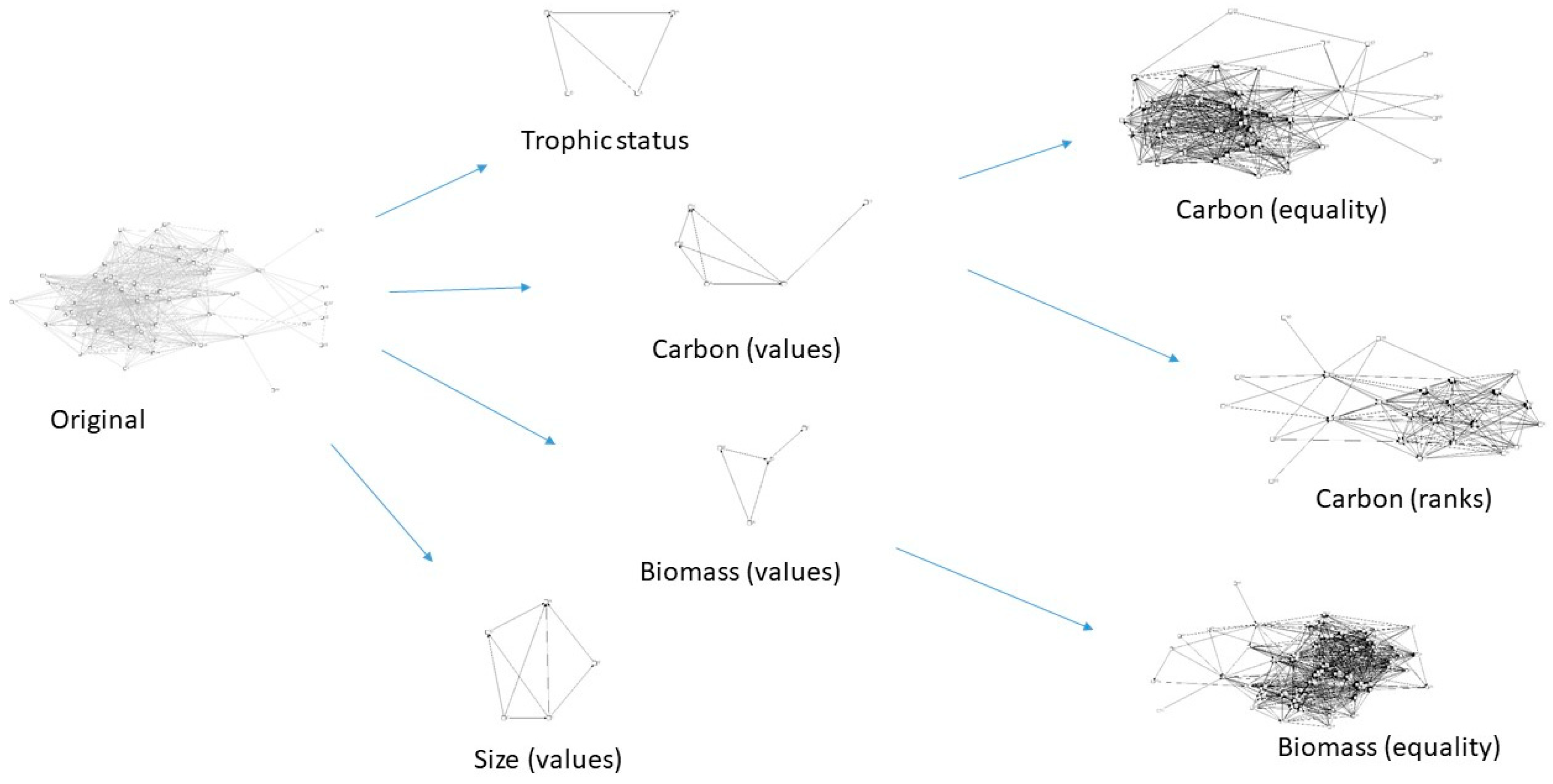
2. Materials and Methods
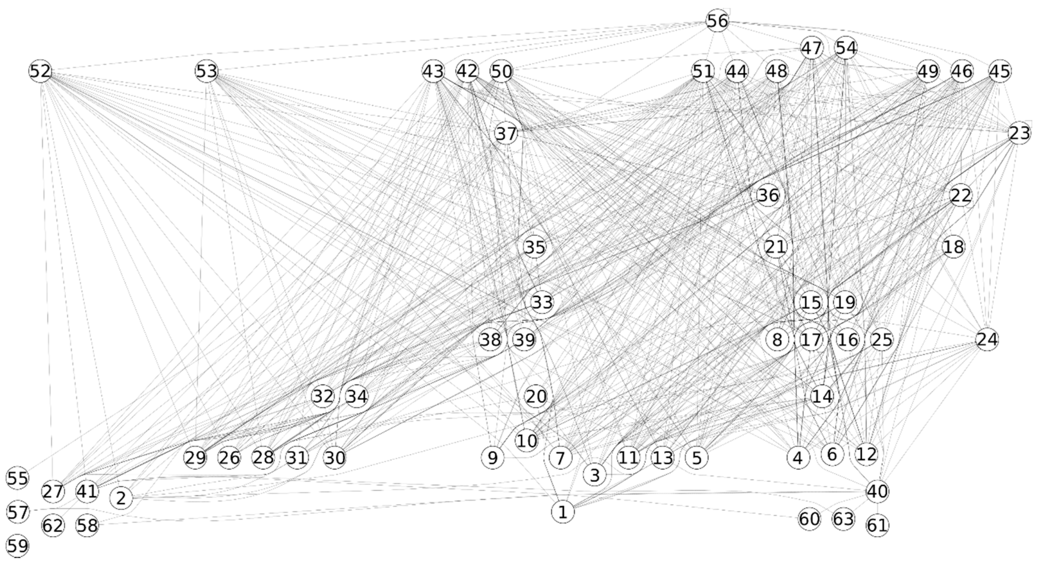
2.1. Data

For illustration, we use a toy network (Figure 1) and a real food web (Figure 2). The real food web describes the oligotrophic state of Gulf of Naples, as sampled at the Long-Term Ecological Research station MareChiara (LTER-MC, [20]). This network describes the planktonic food web composed of phytoplankton (autotrophic unicellular organisms), micro-zooplankton (phago-trophic unicellular organisms), and meso-zooplankton (small invertebrates) [21,22]. The level of trophic resolution in the network is much higher than the average since a large amount of biological information is available for all planktonic organisms in the ecosystem.
The main property of the plankton food web investigated therein is the low specialization of organisms resulting in a marked, though partial, trophic redundancy in most functional nodes. The effort made in producing a network-model for the Gulf of Naples plankton [21] was directed toward integrating trophic diversity and community functioning: Therefore, taxonomic aggregation was limited to the aggregation of abundances of sibling species (i.e., belonging to the same biological genus) that formed a unique functional node in the resulting network. By taking the latter option, functional nodes included organisms having the same trophic properties.

2.2. Methods

In both networks, we analyzed the similarity of network nodes based on the overlap in direct and indirect interactions (TO, STO) and regular equivalence (REGE). While TO and STO consider undirected networks, the REGE approach is based on directed predator-prey interactions. The former method expresses the number of shared preys and predators and quantifies unique vs. redundant food web positions in this sense. The latter method quantifies feeding types and guild identity. These approaches are described below.

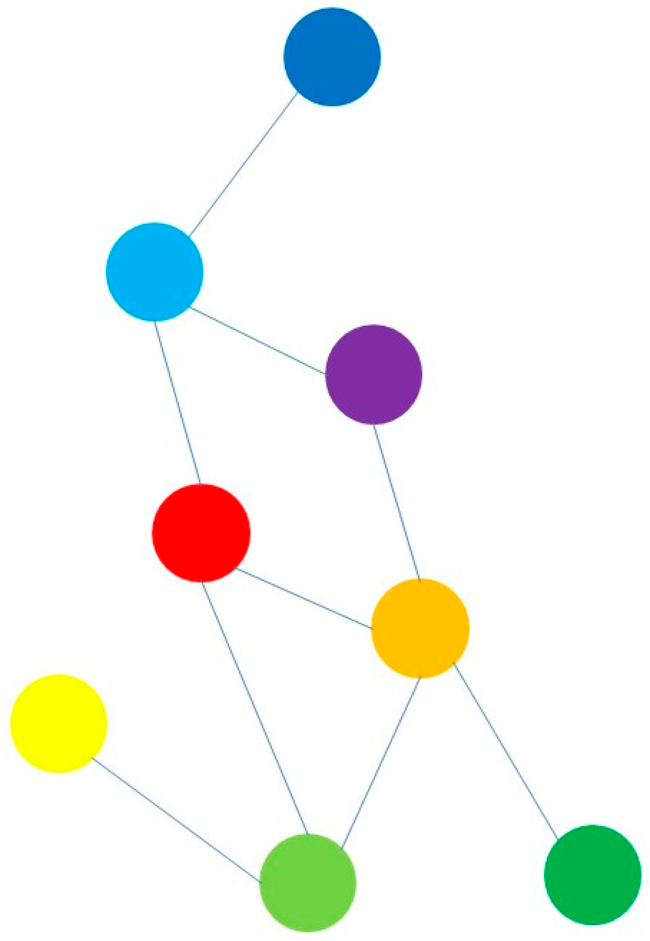
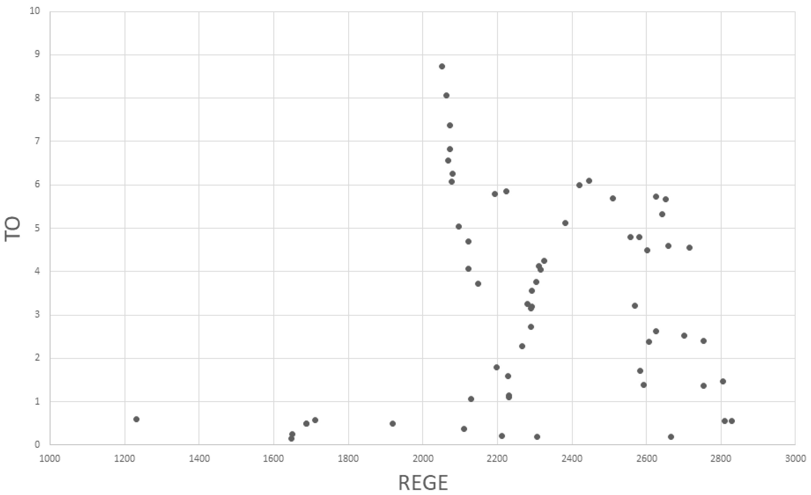
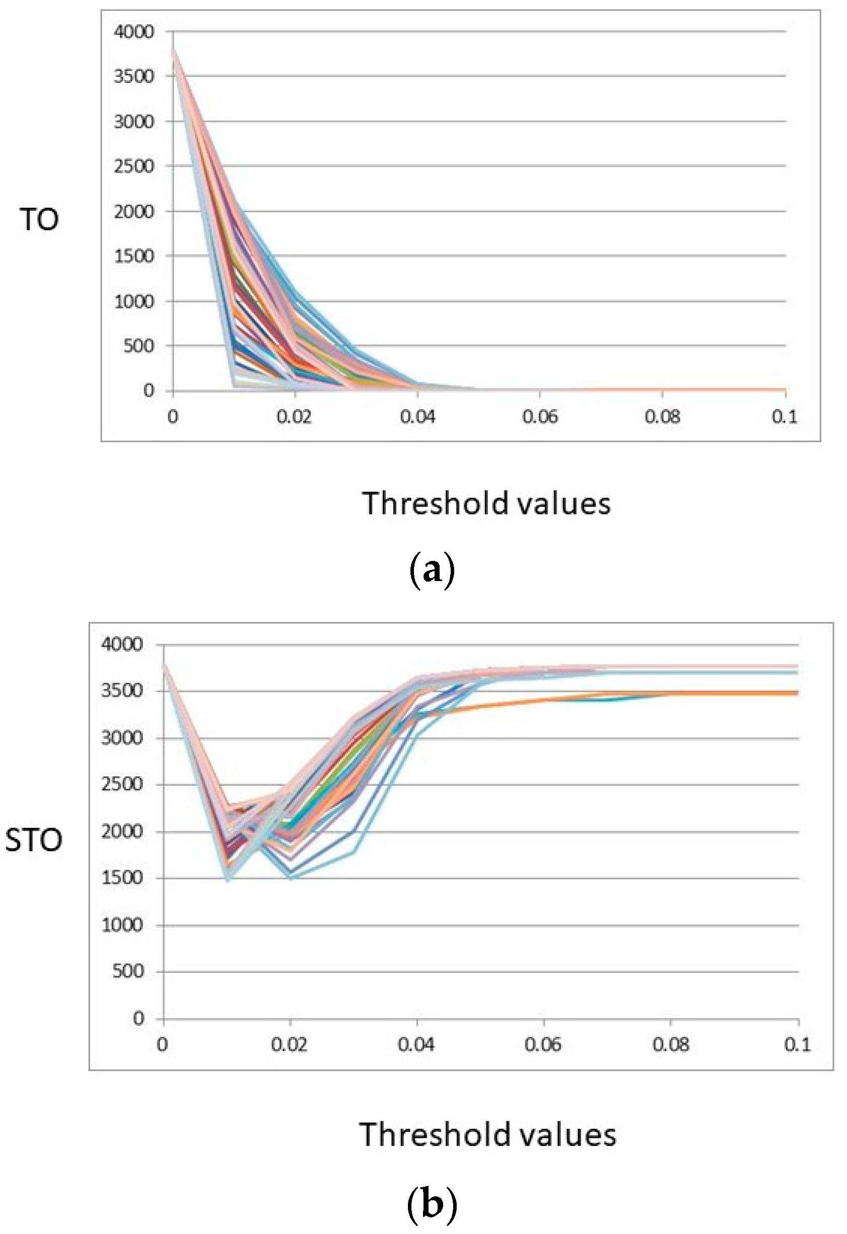
2.2.1. Topological Overlap (TO, STO)

Müller et al. [23] developed a methodology for quantifying the interaction strength between species in a host-parasitoid community and Jordán et al. [24] later then generalized such an approach for food webs. The principle here is that one species can affect the other via direct interaction and via indirect pathways.
Let us consider a food web of N species, and if two species i and j are connected then the direct effect of i on j (or the one-step effect) is:
a i j = 1 D j ,
where Dj is the number of nodes directly connected to j (i.e., its degree). Here, i strongly affects j if i is j’s only neighbor; whereas i can only affect j weakly if j has many neighbors. We then construct a square matrix A(1) where the ijth element, A(1)ij, is the one step effect of i on j. Two-step effects between species can be quantified by using matrix multiplication:
A ( 1 ) × A ( 1 ) = A ( 1 ) 2 = A ( 2 ) ,
where the ijth element of matrix A(2), namely A(2)ij, is the 2-step effect of i on j. Three-step effects can be obtained by calculating A(1)3 (i.e., resulting in matrix A(3)), and in general we only need to calculate A(1)n for n-step effects (i.e., resulting in matrix A(n)).
The matrix A(n) contains some interesting information. It can be partitioned into two matrices:
A ( n ) = Q ( n ) + R ( n ) .
In Equation (3), Q(n) is a diagonal matrix where its iith element, Q(n)ii, represents the n-step long self effect of species i on itself. Q(n)ii is non-zero if there exists at least one loop of length n linking species i to itself. R(n) is a hollow matrix where its ijth element, R(n)ij, is the n-step long effect of species i on species j. R(n)ij is non-zero if there exists at least one pathway of length n linking species i and j. Both Q(n)ii and R(n)ij can be partitioned into effects associated with individual pathways. For instance, consider a simple food web with 4 species where species i consumes species k and h, and both species k and h in turn consume species j. For n = 2, the 2-step long self-effect of species i on itself is:
Q ( 2 ) i i = a i k a k i + a i h a h i .
In Equation (4), aikaki is the effect associated with the pathway “node i–node k–node i”, which is the product of two direct effects (i.e., the direct effect of i on k and the direct effect of k on i); and aihahi is the effect associated with the pathway “node i–node h–node i”, which is also the product of two direct effects (i.e., the direct effect of i on h and the direct effect of h on i). Similarly, the 2-step long effect of species i on species j is:
R ( 2 ) i j = a i k a k j + a i h a h j ,
where aikakj is the effect associated with the pathway “node i–node k–node j” and aihahj is the effect associated with the pathway “node i–node h–node j”.
Since there may be several paths of various lengths between two given species i and j in a food web, we can quantify the average effects of species i on j up to path length n:
E ( n ) i j = 1 n ( A ( 1 ) i j + A ( 2 ) i j + A ( 3 ) i j + A ( n ) i j )
We then construct an interaction matrix E(n), where the ijth element is E(n)ij. Given the way how E(n)ij is defined, its value therefore falls within the interval [0, 1]. Taking the advantage of the interaction matrix E(n), we can quantify the positional uniqueness of individual species as follows [25]. First, for a threshold effect size T, we construct an interactor matrix MT. The ijth element of this matrix, MTij, takes the label S if MTij > T (i.e., j is i’s strong interactor); if not then MTij takes the label W (i.e., j is i’s weak interactor). The ith row of matrix MT can be considered as the interactor profile of species i, which indicates what type of interactor (strong or weak) another species is to species i. Second, for a species pair ij, we compare the ith row with the jth row of the matrix MT; and the number of “S” matches, namely TOTij, is a measure of trophic overlap between species i and j. A large TOTij value indicates species i and j share many strong interactors, whereas a small value says that they share few strong interactors. After all TOT values have been computed for all species pairs, we then put them in a square matrix TOT where the ijth element is TOTij. Finally, the extent of trophic overlap between species i and all other species in the same food web, namely TOTi, can be quantified by summing up the ith row of the TOT matrix. A given species i is truly unique if it has a small TOTi value, because it shares fewer strong interactors with all other species in the same food web (e.g., an aggregated trophic guild); whereas a large TOTi indicates the redundancy of species i’s role in the interaction structure of the food web (e.g., many generalist species).
This method can be improved by taking into account all information in species’ interactor profiles. Here, TOTij is now the number of “S” matches plus the number of “W” matches between the ith and the jth rows of the matrix MT. In other words, we now define the extent of trophic overlap between species i and j by counting the number of strong and weak interactors they have in common. As before, the sum of the ith row (TOTi) of matrix TOT is the unique value of species i for threshold effect size T. A different T value results in a different TOT matrix and therefore gives a different uniqueness value for species i (i.e., TOTi). Thus, a better uniqueness measure should take into consideration information derived from different T values. Since the minimum and the maximum values of an element of the interaction matrix E(n) are 0 and 1 respectively, we only need to explore T within the interval [0, 1] by using a suitable increment value. A suitable increment value of T is chosen such that any smaller increment values don’t change the outcome of our analysis. Here, we systematically vary T from 0 to 1 in increments of, for example, 0.001. When T = 0, all species will have the same strong interactors (as they have no weak interactors) and they will have the same species uniqueness values (i.e., TOTi). As we move T away from 0, TOTi values will start to diverge. Those TOTi values will be most heterogeneous when T reaches a certain value, and beyond which TOTi values will then converge. When T = 1, all species will have the same species uniqueness values as they all have the same weak interactors (and they have no strong interactors). This extreme situation would mean that each species in an ecological community is largely independent of the others (or only very weakly influenced by them).
For each species i, a unique TO profile can be obtained when TOTi is plotted against different values of T; and the sum of all TOTi values across the entire range of T values is now the new measure for species i’s uniqueness (STOi). A unique species tend to have a small STOi value as it has few strong and weak interactors in common with all other species across the entire range of T values [26]. This describes a situation when, for example, a herbivore feeds on rare plants and do not consume abundant, dominant plants consumed by many others.

2.2.2. Regular Equivalence (REGE)

The positional similarity of network nodes can be calculated by using the regular equivalence measure (REGE, [6,27,28]). This measure quantifies the similarity between the positions of network nodes i and j based on their network neighborhood. Briefly, two nodes are said to be regular equivalent if they are connected with the same types of nodes. In ecology terms, two species are more regularly equivalent if they have similar (but not necessarily the same) predators and preys: For example, two canopy insects feeding on leaves of different trees and consumed by different bird species. A REGE matrix S is the output of such an analysis, where the ijth element, Sij, expresses the extent of similarity between nodes i and j. An iterative algorithm is used to determine S [6]. First, we define a N × N matrix R(t) whose ijth element, R(t)ij, is the extent of regular equivalence between i and j at iteration t. Second, we carry out the following procedures:
  • At iteration 0, all node pairs are perfectly equivalent (i.e., R(0)ij = 1).
  • At iteration t + 1, the extent of regular equivalence between i and j, R(t + 1)ij, is determined as follows.
    (a)
    For outgoing links only, for each neighbor k of i (i.e., species i and its predator k), we determine which neighbor m of j (i.e., species j and its predator m) that is most equivalent to k according to R(t) (i.e., the largest R(t)km); and then we define a quantity Xi,k,j which takes the value of R(t)km. Likewise, from the perspective of j, we determine the value of Xj,m,i.
    (b)
    For incoming links only, for each neighbor h of i (i.e., species i and its prey h), we determine which neighbor n of j is most equivalent to h according to R(t) (i.e., the largest R(t)hn); and we then define a quantity Yi,h,j which takes the value of R(t)hn. Similarly, from the perspective of j, one determines the value of Yj,n,i.
    (c)
    The extent of regular equivalence between i and j at iteration t + 1 is defined as:
    R ( t + 1 ) i j = k X i , k , j + m X j , m , i + h Y i , h , j + n Y j , n , i M A X ( k X i , k , j + m X j , m , i + h Y i , h , j + n Y j , n , i ) ,
    where the denominator is the maximum possible value of the numerator if i and j are perfectly equivalent. R(t + 1)ij is bounded between 0 and 1, with 1 indicating i and j are perfectly equivalent.
  • We repeat procedure 2 after a predefined number of iterations and let matrix S be the final R(t + 1) matrix.
The sum of the ith row of matrix S provides a measure of redundancy. Beyond numerical results, we illustrate the similarities for all nodes by using a dendrogram. This dendrogram can be cut at any threshold level in order to define and create aggregated functional groups. An analysis was carried out by using the UCINET software [29]. Similar approaches have already been suggested in ecology (cf. tropho-species [7,30]).

2.2.3. Trait-Based Similarity Measures
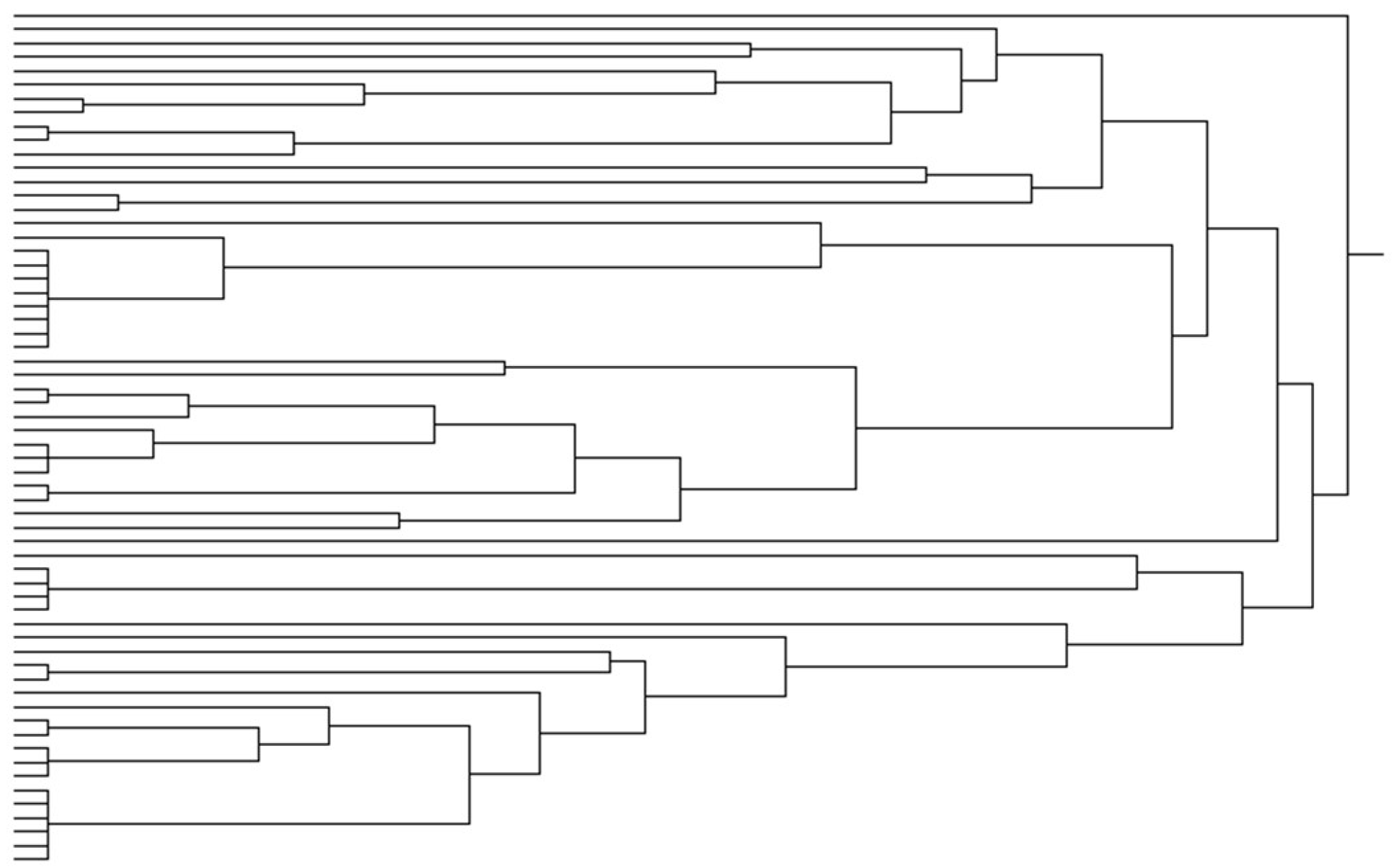
For real networks, biological information is also available for characterizing graph nodes. These are (recently) called “traits”; large trait databases are meant to create the chance for the future “big data ecology”. We used 3 traits (b for biomass, s for size and c for carbon content) and used each of them for aggregation in 3 ways. Carbon content and biomass are generally correlated, yet we used both traits as carbon content is an individual-level property (i.e., quantifying the body mass of a single individual belonging to a functional node), while biomass is a population-level property (i.e., quantifying the overall mass of a functional node). We (1) aggregated species with equal trait values (e for equal), (2) aggregated species belonging to 30 evenly defined range of traits values (v for value) and (3) aggregated species based on their trait value ranks in groups of 3 (r for rank). Out of the 9 possible combinations only 6 seemed to be relevant for further analysis (sv, ce, cr, cv, be, bv): Three other possibilities were not considered, because of measurement problems (se and sr) and providing irrelevant information (br). In each case, aggregated groups were named by letters (while numbers refer to the original trophic groups in References [21,22]). Finally, we aggregated the species also by their trophic status (ts, with categories like autotrophs (coded as A), mixotrophs (M), heterotrophs (H) and detritivores (D). Altogether, the above-mentioned procedures provided 7 ways of aggregation and 7 low-resolution, aggregated food webs.

3. Results

In the toy network (Figure 1), the computation of the REGE half-matrix (Table 1B) is based on the adjacency matrix (Table 1A) and the calculations of the TO2;0.15 half-matrix (n = 2, T = 0.15; Table 1D) is based on the TI2-matrix (Table 1C). For both REGE and TO, a ranking of graph nodes can be given (Table 1B,D, on the left). Nodes r (red) and o (orange) are in the most redundant positions according to both approaches. The rank of node p (purple) shows the largest difference: REGE suggests that its topological position is more redundant, while TO suggest it to be more unique. Based on REGE (Figure 3), its position is quite similar to that of node r (red), but TO considers the difference larger, because of the link between r (red) and lg (light green).
For the food web of Gulf of Naples (Figure 2), the computation of the REGE half-matrix (Table S1b) is based on the adjacency matrix (Table S1a), and the calculation of the TO2;0.02 half-matrix (Table S1d) is based on the TI2-matrix (Table S1c). For both REGE and TO, a ranking of graph nodes can be given (Table S1b,d, on the left). Nodes #31 #16 and #13 are in the most redundant positions according to REGE (see also Figure 4), and nodes #51, #42 and #46 are the most redundant ones according to TO. Interestingly, while the two approaches show quite a coincidence for the small toy network, the ranks are very different for this much larger web (see Figure 5). Yet, for the end of the ranks (the less redundant, more unique topological positions), the coincidence is much stronger (#56, #61 and #60 for REGE and #61, #55 and #20 for TO, see Table S1b,d, from the bottom up).
For this latter network, we studied two additional features of the aggregation process. One potential reason for the difference is the inappropriate use of the threshold value for calculating TOn (for both networks, so far, the average of all TI-values was used, rounded up to second decimal). TO-values for different thresholds are shown in Table S2 and visualized in Figure 6a. Another potential reason is that STO may provide different results. Table S3 shows the nodal STO-values visualized in Figure 6b. Table S4 shows the biological organisms represented by the graph nodes of the Gulf of Naples food web.
Following the mathematical analysis of node similarity, we take a trait-based view and use biological knowledge for defining similar nodes and aggregate the network accordingly. In Figure 7, we show all aggregated versions of the original food web, shown in Figure 2. Aggregating according to trophic status (ts), the results are quite trivial: Heterotrophs and mixotrophs consume detritus and autotrophs. According to aggregation based on carbon values (cv), we get 5 nodes like A: #49 (juvenile Calanoids), B: #54 (Oithona spp), C: #56 (carnivores), D: #52 (salps) and E: everything else. According to biomass values (bv), we have A: #62 (generic particulate detritus), B: #41 (heterotrophic bacteria), C: #29 (coccolithophorids) and #56 (carnivores) and D: everything else. According to size values (sv), we have A: #56 (carnivora), B: #52 (salps), C: #50 (Appendicularia) and #57 (Appendicularia houses), D: #45 (Acartia clausii) and #46 (Temora stylifera) and #47 (Centropages typicus) and #48 (other calanoids) and #51 (doliolids), E: Everything else. According to carbon equality (ce), carbon ranks (cr) and biomass equality (be), most groups remain un-aggregated. The most unique nodes can be seen in Table 2.
When comparing the most unique network positions based on REGE (e.g., #56), TO (e.g., #60), STO (e.g., #51) and trait-based aggregations (e.g., #56), we derived the following conclusions: (i) The relationship between TO and STO was quite sensitive to the threshold used—i.e., when the latter is set between 0.01 and 0.02, this relationship changes sign and it becomes continuously weaker (Figure S5); (ii) REGE correlates a little better with TO (Figure S6) than with STO (Figure S7); and (iii) in both cases, changing the threshold results in quantitative effects, but not in qualitative ones.
The organisms that were unaffected by the bv type of trait-based aggregations could be characterized by any specific combination of TO and REGE (Figure S8). Separation on the TO/REGE plain was better for cv (Figure S9) and especially sv (Figure S10). Similar results hold for the STO/REGE plain for bv (Figure S11), cv (Figure S12) and sv (Figure S13).

4. Discussion

Aggregating taxa to manage ecological complexity and, at the same time, reduce computational complexity is a key issue of ecology studies on plankton food-webs, like the one investigated herein. This need stems from the huge diversity of microscopic organisms present in aquatic environments, even in small water volumes [31]. Based on our results, aggregating planktonic organisms by size values appears as the best option among the available ones, since it allows partially matching the need to produce a reliable food-web including ecologically relevant planktonic consumers. Yet, a sufficient coverage for trophic behavior is not fully accomplished by aggregating by trophic status or biomass, while carbon-aggregation can be useful to some extent.
Most plankton models published so far tended to compress plankton diversity within few trophic groups, owing to a longstanding tradition based on a very simple representation of a plankton trophic chain including inorganic nutrients as an input for a single phytoplankton group and the latter being food for a single zooplankton group (i.e., the so-called NPZ modelling scheme, [32]). Conceptual advancements indicate the importance of expanding the biological resolution in plankton models by separating between micro- (size < 200 µm) and meso- (200 µm < size < 2 cm, approximately) -plankton and also by distinguishing between a number of meso-zooplankton sub-groups characterized by distinct trophic behaviors [33].
Our mathematical study suggests that size-aggregation can give rise to functional nodes representing, although partially, all the major trophic levels in the plankton food web of the Gulf of Naples, with an opportune expansion in the meso-zooplankton assemblage that results aggregated in 4 nodes, as follows: (A) Carnivores (#56); (B) salps (#52); (C) Appendicularia and Appendicularia houses (#50,57), (D) Acartia clausii, Temora stylifera, Centropages typicus, other calanoids, doliolids (#45–48,51) (Figure 7). A partial reliability of size aggregation in the plankton food-web stems from the comparison between the results of the present mathematical effort and the ecological properties of the plankton food-web analyzed, which are synthesized in previous works [21,22]. Such a comparison is summarized below.
Firstly, carnivores in the Gulf of Naples food-web (A) are represented mainly by arrow-worms (Chaetognata), which set at the highest trophic level and have a considerably different trophic behavior from all the other nodes represented in the aggregated web. Salps and Appendicularia (B,C) mainly feed on microbes and they set at a lower trophic rank in respect to carnivores; they both are filter-feeders of small plankton particles, but, by being of different sizes, they fall into different nodes and this discrimination captures correctly their slightly different affinities for microbes of different sizes [34]. Appendicularia houses (#57) are opportunely considered in the (C) node, since they constitute a particular detritus-form derived from living Appendicularia individuals. Calanoid copepods (Crustacea, D) set well all together since they are reciprocally closely related, show very plastic diets, in comparison with animals in B and C, which are more focused on small particles. Nonetheless, doliolids, which are more closely related with salps and Appendicularia, are aggregated together with copepods and this can represent a limit to size aggregation.
For the reasons shown above, the analytical approaches presented herein can set an opportune threshold for the aggregation of meso-zooplanktonic animals. When coupled with food-web topology, size-based aggregation is an apparently effective criterion for isolating some of the main meso-zooplankton nodes. In addition to size, carbon-based aggregation can also help identify some other important groups with particular trophic characteristics, like Oithona spp. (#54), which have a relatively small carbon value, but a relatively high trophic position—i.e., they eat on other meso-zooplankton. Herein, we evaluated various ways of aggregation focusing on single particular traits—but combining different traits seems to be a further opportune direction.
One might by the way notice in the analyses shown herein the general aggregation of microbial plankton, from phyto- to micro-zooplankton, in one and a single functional node: This is an important limit of all the aggregation criteria followed herein. Previous researches remark the fundamental role of heterotrophic and mixotrophic (i.e., contemporarily photosynthetic and phagotrophic) micro-zooplankton in driving plankton food-webs [35]. Therefore, it may be helpful to repeat the aggregation exercise herein presented but limiting the analyses to the sole functional node E, i.e., the one aggregating everything but some meso-zooplankton nodes according to the size-criterion. Furthermore, one should investigate further the opportunity to aggregate cladocerans (Crustacea #42,43) all in the E group: At first glance, this option may be justified by the relatively small size and carbon content of these animals in comparison with the other meso-zooplankton and they also have a diet similar to micro-zooplankton. In future studies, more detailed demographic information of each species should be considered in the aggregation process. These include physiological characteristics, such as growth rate, reproductive strategy and generation time. Aggregation based on these criteria is important in studying the behavior of dynamic models as different aggregation strategies surely result in different functional groups being modelled and consequently resulting in different model dynamics. Finally, future analyses may be considering weighted networks produced based on trophic flows, which can provide more realistic results.
Our systemic view provides a quantitatively holistic view on the structure of ecosystems. Earlier studies have shown that REGE can result in taxonomically both homogeneous and heterogeneous groups [14]: Heterogeneous groups can reveal ecological functional similarity not reflected in taxonomic closeness. We are suggesting that comparing biological and mathematical definitions of similarity and the consequent aggregation methods can provide standards and, at the same time, consider biological knowledge for better understanding of ecological functionality. Based on a single case study, we prefer not to make major statements. It is still a long way to go if we really want to understand (1) how are mathematical and trait-based aggregations related to each other and (2) how to use mathematics in order to replace (predict) biological aggregation if big databases are lacking.

Supplementary Materials

The following are available online at https://www.mdpi.com/2227-7390/6/12/336/s1. Table S1: The adjacency matrix (A), the REGE half matrix (B), the TI matrix (C) and the TO half matrix for the Gulf of Naples network. For REGE and TO we also present the ranking of the nodes. Table S2: The ranking of nodes based on their TO-values for different thresholds (T = 0.01, 0.02, 0.03, 0.04, 0.05, 0.06). Table S3: The ranking of nodes based on their STO-values for different thresholds (T = 0.01, 0.02, 0.03, 0.04, 0.05, 0.06). Table S4: The identity of graph nodes in the Gulf of Napoli food web. Figure S1: Correlations between TO and STO for several threshold values. Figure S2: Correlations between TO and REGE for several threshold values. Figure S3: Correlations between STO and REGE for several threshold values. Figure S4: The position of the not aggregated (A: #62; B: #41) or only weakly aggregated (C: #29 and #56) trophic groups in the TO/REGE plain. All organisms aggregated into E (everything else) are shown. Based on the “bv” aggregation (see Table 2). The plots are shown for 6 threshold values. Figure S5: The position of the not aggregated (A: #49; B: #54; C: #56; D: #52) trophic groups in the TO/REGE plain. All organisms aggregated into E (everything else) are shown. Based on the “cv” aggregation (see Table 2). The plots are shown for 6 threshold values. Figure S6: The position of the not aggregated (A: #56; B: #52) or only weakly aggregated (C: #50 and #57; D: #45, #46, #47, #48 and #51) trophic groups in the TO/REGE plain. All organisms aggregated into E (everything else) are shown. Based on the “sv” aggregation (see Table 2). The plots are shown for 6 threshold values. Figure S7: The position of the not aggregated (A: #62; B: #41) or only weakly aggregated (C: #29 and #56) trophic groups in the STO/REGE plain. All organisms aggregated into E (everything else) are shown. Based on the “bv” aggregation (see Table 2). The plots are shown for 6 threshold values. Figure S8: The position of the not aggregated (A: #49; B: #54; C: #56; D: #52) trophic groups in the STO/REGE plain. All organisms aggregated into E (everything else) are shown. Based on the “cv” aggregation (see Table 2). The plots are shown for 6 threshold values. Figure S9: The position of the not aggregated (A: #56; B: #52) or only weakly aggregated (C: #50 and #57; D: #45, #46, #47, #48 and #51) trophic groups in the STO/REGE plain. All organisms aggregated into E (everything else) are shown. Based on the “sv” aggregation (see Table 2). The plots are shown for 6 threshold values.

Author Contributions

Conceptualization, F.J.; Data curation, D.D.A.; Investigation, A.E.; Methodology, F.J. and W.-c.L.; Software, W.-c.L.; Supervision, F.J.; Visualization, D.D.A.; Writing—original draft, F.J.; Writing—review and editing, F.J., A.E., W.-c.L. and D.D.A.

Funding

The work of A.E. and F.J. was funded by National Research, Development and Innovation Office—NKFIH, grant number OTKA K 116071. The work of F.J. was funded by the grant GINOP-2.3.2-15-2016-00057. The work of D.D.A. was funded by the Flagship Project RITMARE—The Italian Research for the Sea—funded by the Italian Ministry of Education, University, and Research within the National Research Program 2011–2013.

Acknowledgments

We are grateful to the participants of the DynaTrait conference in Hannover (October 2017) for some initial discussions. Three anonymous reviewers are acknowledged for helpful and constructive comments.

Conflicts of Interest

The authors declare no conflict of interest.

References

  1. Martinez, N.D. Artifacts or attributes? Effects of resolution on the Little Rock Lake food web. Ecol. Monogr. 1991, 61, 367–392. [Google Scholar] [CrossRef]
  2. Thompson, R.M.; Brose, U.; Dunne, J.A.; Hall, R.O.; Hladyz, S.; Kitching, R.L.; Martinez, N.D.; Rantala, H.; Romanuk, T.N.; Stouffer, D.B.; et al. Food webs: Reconciling the structure and function of biodiversity. Trends Ecol. Evol. 2012, 27, 689–697. [Google Scholar] [CrossRef] [PubMed]
  3. Power, M.E.; Tilman, D.; Estes, J.A.; Menge, B.A.; Bond, W.J.; Mills, L.S.; Daily, G.; Castilla, J.C.; Lubchenco, J.; Paine, R.T. Challenges in the quest for keystones. BioScience 1996, 46, 609–620. [Google Scholar] [CrossRef]
  4. Lawton, J.H.; Brown, V.K. Redundancy in ecosystems. In Biodiversity and Ecosystem Function; Schulze, E.D., Mooney, H.A., Eds.; Springer: Berlin, Germany, 1994; pp. 255–270. [Google Scholar]
  5. Cohen, J.E. Food Webs and Niche Space; Princeton University Press: Princeton, NJ, USA, 1978. [Google Scholar]
  6. Luczkovich, J.J.; Borgatti, S.P.; Johnson, J.C.; Everett, M.G. Defining and measuring trophic role similarity in food webs using regular equivalence. J. Theor. Biol. 2003, 220, 303–321. [Google Scholar] [CrossRef] [PubMed]
  7. Cirtwill, A.R.; Dalla Riva, G.V.; Gaiarsa, M.P.; Bimler, M.D.; Cagua, E.F.; Coux, C.; Dehling, D.M. A review of species role concepts in food webs. Food Webs 2018. [Google Scholar] [CrossRef]
  8. Hall, S.J.; Raffaelli, D. Food-web patterns: Lessons from a species-rich web. J. Anim. Ecol. 1991, 60, 823–841. [Google Scholar] [CrossRef]
  9. Goldwasser, L.; Roughgarden, J. Construction and analysis of a large caribbean food web. Ecology 1993, 74, 1216–1233. [Google Scholar] [CrossRef]
  10. Hirata, H.; Ulanowicz, R.E. Information theoretical analysis of the aggregation and hierarchical structure of ecological networks. J. Theor. Biol. 1985, 116, 321–341. [Google Scholar] [CrossRef]
  11. Pahl-Wostl, C. The possible effects of aggregation on the quantitative interpretation of flow patterns in ecological networks. Math. Biosci. 1992, 112, 177–183. [Google Scholar] [CrossRef]
  12. Solow, A.R.; Beet, A.R. On lumping species in food webs. Ecology 1998, 79, 2013–2018. [Google Scholar] [CrossRef]
  13. Jordán, F.; Osváth, G. The sensitivity of food web topology to temporal data aggregation. Ecol. Model. 2009, 220, 3141–3146. [Google Scholar] [CrossRef]
  14. Patonai, K.; Jordán, F. Aggregation of incomplete food web data may help to suggest sampling strategies. Ecol. Model. 2017, 352, 77–89. [Google Scholar] [CrossRef]
  15. Scotti, M.; Hartvig, M.; Winemiller, K.O.; Li, Y.; Jauker, F.; Jordán, F.; Dormann, C.F. Trait-based and process-oriented modeling in ecological network dynamics. In Adaptive Food Webs; Moore, J.C., de Ruiter, P.C., McCann, K.S., Wolters, V., Eds.; Cambridge University Press: Cambridge, UK, 2017; pp. 228–256. [Google Scholar]
  16. Sommer, U.; Charalampous, E.; Scotti, M.; Moustaka-Gouni, M. Big fish eat small fish: Implications for food chain length? Comm. Ecol. 2018, 19, 107–115. [Google Scholar] [CrossRef]
  17. Bond, W.J. Keystone species. In Biodiversity and Ecosystem Function; Schulze, E.D., Mooney, H.A., Eds.; Springer: Berlin, Germany, 1994. [Google Scholar]
  18. Daily, G.C.; Ehrlich, P.R.; Haddad, N.M. Double keystone bird in a keystone species complex. Proc. Natl. Acad. Sci. USA 1993, 90, 592–594. [Google Scholar] [CrossRef] [PubMed]
  19. Ortiz, M.; Hermosillo-Nuñez, B.; González, J.; Rodríguez-Zaragoza, F.; Gómez, I.; Jordán, F. Quantifying keystone species complexes: Ecosystem-based conservation management in the King George Island (Antarctic Peninsula). Ecol. Indic. 2017, 81, 453–460. [Google Scholar] [CrossRef]
  20. d’Alcalà, M.R.; Conversano, F.; Corato, F.; Licandro, P.; Mangoni, O.; Marino, D.; Mazzocchi, M.G.; Modigh, M.; Montresor, M.; Nardella, M.; et al. Seasonal patterns in plankton communities in a pluriannual time series at a coastal Mediterranean site (Gulf of Naples): An attempt to discern recurrences and trends. Sci. Mar. 2004, 68, 65–83. [Google Scholar]
  21. D’Alelio, D.; Libralato, S.; Wyatt, T.; Ribera d’Alcalà, M. Ecological-network models link diversity, structure and function in the plankton food-web. Sci. Rep. 2016, 6, 21806. [Google Scholar] [CrossRef] [Green Version]
  22. D’Alelio, D.; Montresor, M.; Mazzocchi, M.G.; Margiotta, F.; Sarno, D.; Ribeira d’Alcalà, M. Plankton food-webs: To what extent can they be simplified? Adv. Oceanogr. Limnol. 2016, 7. [Google Scholar] [CrossRef]
  23. Müller, C.B.; Adriaanse, I.C.T.; Belshaw, R.; Godfray, H.C.J. The structure of an aphid–parasitoid community. J. Anim. Ecol. 1999, 68, 346–370. [Google Scholar] [CrossRef]
  24. Jordán, F.; Liu, W.-C.; van Veen, F.J.F. Quantifying the importance of species and their interactions in a host-parasitoid community. Commun. Ecol. 2003, 4, 79–88. [Google Scholar] [CrossRef]
  25. Jordán, F.; Liu, W.-C.; Mike, Á. Trophic field overlap: A new approach to quantify keystone species. Ecol. Model. 2009, 220, 2899–2907. [Google Scholar] [CrossRef]
  26. Lai, S.M.; Liu, W.C.; Jordán, F. A trophic overlap-based measure for species uniqueness in ecological networks. Ecol. Model. 2015, 299, 95–101. [Google Scholar] [CrossRef]
  27. Lorrain, F.; White, H.C. Structural equivalence of individuals in social networks. J. Math. Sociol. 1971, 1, 49–80. [Google Scholar] [CrossRef]
  28. Everett, M.G.; Borgatti, S. Role colouring a graph. Math. Soc. Sci. 1991, 21, 183–188. [Google Scholar] [CrossRef]
  29. Borgatti, S.P.; Everett, M.G.; Freeman, L.C. Ucinet for Windows: Software for Social Network Analysis; Analytic Technologies: Harvard, MA, USA, 2002. [Google Scholar]
  30. Yodzis, P.; Winemiller, K.O. In search of operational trophospecies in a tropical aquatic food web. Oikos 1999, 87, 327–340. [Google Scholar] [CrossRef]
  31. Carradec, Q.; Coordinators, T.O.; Pelletier, E.; Da Silva, C.; Alberti, A.; Seeleuthner, Y.; Blanc-Mathieu, R.; Lima-Mendez, G.; Rocha, F.; Tirichine, L.; et al. A global ocean atlas of eukaryotic genes. Nat. Commun. 2018, 9, 373. [Google Scholar] [CrossRef] [PubMed] [Green Version]
  32. Franks, P.J.S. NPZ models of plankton dynamics: Their construction, coupling to physics, and application. J. Oceanogr. 2002, 58, 379–387. [Google Scholar] [CrossRef]
  33. Mitra, A.; Castellani, C.; Gentleman, W.C.; Jonasdottir, S.H.; Flynn, K.J.; Bode, A.; Halsband, C.; Kuhn, P.; Licandro, P.; Agersted, M.D.; et al. Bridging the gap between marine biogeochemical and fisheries sciences; configuring the zooplankton link. Progr. Oceanogr. 2014, 129, 176–199. [Google Scholar] [CrossRef]
  34. Conley, K.R.; Lombard, F.; Sutherland, K.S. Mammoth grazers on the ocean’s minuteness: A review of selective feeding using mucous meshes. Proc. Biol. Soc. 2018, 285, 20180056. [Google Scholar] [CrossRef]
  35. Flynn, K.J.; Stoecker, D.K.; Mitra, A.; Raven, J.A.; Glibert, P.M.; Hansen, P.J.; Granéli, E.; Burkholder, J.M. Misuse of the phytoplankton–zooplankton dichotomy: The need to assign organisms as mixotrophs within plankton functional types. J. Plankton Res. 2012, 35, 3–11. [Google Scholar] [CrossRef]
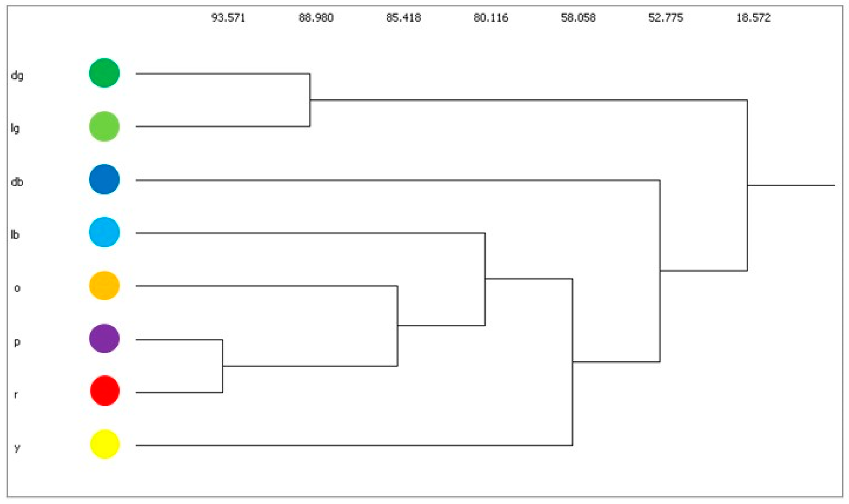
Figure 1. A toy food web for illustration. The dark blue and the yellow nodes are top-predators and the light green and dark green nodes are the producers. The direction of carbon flows is not shown (from the bottom upwards) for simplicity.
Mathematics 06 00336 g001
Figure 2. The food web of the Gulf of Naples at LTER-MC.
Mathematics 06 00336 g002
Figure 3. The REGE-based similarity dendrogram for the toy network, shown in Figure 1. The x-axis shows the similarity of network positions: The path is shorter between similar nodes. Nodes are marked by both colors and abbreviations (dg, dark green; lg, light green; db, dark blue; lb, light blue; o, orange; p, purple; r, red; y, yellow).
Mathematics 06 00336 g003
Figure 4. The REGE-based similarity dendrogram for the Gulf on Naples food web, shown in Figure 2. The sum of horizontal distances shows similarity of network positions: The path is shorter between similar nodes. Node identity is not shown (for technical reasons).
Mathematics 06 00336 g004
Figure 5. The relationship between the REGE and TO values for each node in the Gulf of Naples food web (Figure 2).
Mathematics 06 00336 g005
Figure 6. The TO (a) and STO (b) profile of nodes in the Gulf of Naples food web for different thresholds (T = 0.01, 0.02, 0.03, 0.04, 0.05, 0.06, 0.07, 0.08, 0.09, 0.1). Every node is represented by a colorful curve. Note that for T = 0 we see the maximal value of the indices.
Mathematics 06 00336 g006
Figure 7. On the left, the original food web, shown in Figure 2. In the middle and on the right, its aggregated versions corresponding to 7 different ways of aggregation.
Mathematics 06 00336 g007
Table 1. The adjacency matrix (A), the regular equivalence (REGE) half matrix (B), the TI matrix (C) and the TO half matrix for the toy network. For REGE and TO we also present the ranking of the nodes. Their color code is explained in Figure 3.
A B
dbdglblgoprydbdglblgopry sum rank
db00000000 067028495056db250r420
dg00001000 18895549360dg247o412
lb10000000 3968858353lb346p411
lg00001011 6561510lg305lb346
o00000110 778958o412lg305
p00100000 9445p411db250
r00100000 67r420dg247
y00000000 y223y223
C D
dbdglblgoprydbdglblgopry sum rank
db0.1700.17000.080.060 0200220db6r20
dg00.1300.040.130.060.040 000000dg0o14
lb0.500.640.060,10.250.170 12340lb12lb12
lg00.130.060.260.170.060.210.5 4042lg11lg11
o00.50.140.220.270.250.220.17 152o14p9
p0.170.130.170.040.130.150.10 30p9db6
r0.170.130.170.210.170.150.150.17 2r20y6
y0000.170.0400.060.17 y6dg0
Table 2. The identity of nodes in the not aggregated or only weakly aggregated trophic groups (A, B, C, D) according to 3 different trait-based aggregation procedures (cv, bv, sv; see explanation in the text).
Scenarioscvbvsv
A496256
B544152
C5629, 5650, 57
D52 45, 46, 47, 48, 51
Eothersothersothers

