Research on Spare Part Activation Strategy and Reliability Index Calculation of Cold Standby Voting Systems Under Weibull Distribution

Abstract

This study investigates the impact of standby activation strategies on system reliability. The results show that a delayed activation strategy effectively improves system reliability. Additionally, to tackle the difficulty of deriving analytical solutions for reliability metrics under the Weibull distribution, a non-homogeneous Markov model based on the delayed activation strategy is introduced. The system’s residual life is modeled computationally using the state transition method. The numerical results suggest that the proposed method aligns closely with Monte Carlo simulations. It significantly improves computational efficiency while maintaining high accuracy, thus confirming its effectiveness.

1. Introduction

Cold standby voting systems are fault-tolerant architectures featuring high reliability, flexibility, and scalability. They are widely employed in aerospace systems, nuclear power plant control, and engineering equipment [1,2,3]. The efficient calculation of reliability indices for these systems remains a key area of research. The cold standby voting system $k/n:m(G)$ comprises $n$ operational and $m$ cold standby units, where normal operation is maintained when at least $k$ units are functioning properly. When the number of normally working units decreases from $n$ to $k$ due to component failures, cold standby units can be activated and replace the failed ones, ensuring continued system reliability. $G$ allows for the lifetime distribution of the units to follow any distribution, not limited to exponential distribution, enhancing its relevance to real-world engineering applications.

Extensive studies have been conducted on the reliability of cold standby voting systems. Yang Lechang [4] developed a survival signature-based reliability approach for a multi-state system with both dependence and imprecision developed. The survival function was derived through structural reliability treatments and calculated by two numerical simulation algorithms. Zong Xiaofei [5] analyzed the mean time to failure of such systems using order statistics with a single cold standby, obtaining the system’s mean life under the Weibull distribution via numerical integration. Hu Xinchun [6] derived an analytical formula for the reliability of heterogeneous cold standby voting systems with a single spare part, where the working components follow any distribution. Gu Ruoxing [7] examined typical series, parallel, and voting systems, applying order statistics theory to directly establish a system reliability model that accounts for failure correlations in common load failures. Eryilmaz [8] introduced a weighted reliability calculation method for cold standby voting systems, incorporating components with mixed lifetimes, including two types of active components and one cold standby unit. Zhu Qiyue [9] explored the activation sequence of cold standby parts in the $k/n:m(G)$ cold standby voting system, concluding that in the homogeneous $3/5:2(G)$ cold standby voting system, the delayed activation of cold standby parts improves overall system reliability, though no formal proof was provided. Achintya Roy [10] analyzed the reliability of k-out-of-n systems with two cold standby components, building upon the work of Eryilmaz [11]. Anna [12] developed a Monte Carlo simulation algorithm using stochastic process theory to calculate the mean life of weighted $k/n:m(G)$ voting systems and continuous weighted $k/n:m(G)$ voting systems. Ioannis [13] derived exact formulas for the reliability indices of combined systems consisting of $m$ consecutive $k/n:m(G)$ voting systems and consecutive $k_c/n:m(G)$ voting systems and analyzed the impact of design parameters $m$, $k$, $k_c$ and $n$ on system performance through extensive numerical experiments. Eryilmaz [14] also derived expressions for the survival function and mean time to failure of coherent systems with cold standby components, considering both exponential and non-exponential distributions (e.g., Pareto distribution). Regarding spare part activation strategies, Zhang Bowei [15] proposed a maintenance decision-making method that optimizes spare part ordering and component replacement by predicting the remaining life to trigger spare part deployment, based on intelligent predictions using the C-MAPSS dataset.

Previous studies have provided important insights into reliability modeling and evaluation for cold standby voting systems. However, analytical solutions remain difficult to obtain when lifetimes follow the Weibull distribution, as obtaining analytical expressions for system reliability indices proves difficult. This limitation restricts the practical applicability of the Weibull distribution in such systems. Therefore, this study focuses on determining the optimal spare part activation strategy and calculating reliability indices under the assumption that both component and spare part lifetimes follow the Weibull distribution, aiming to offer valuable theoretical insights and methodological references for the design and application of high-reliability systems.

2. Research on Spare Part Activation Strategy of Cold Standby Systems

2.1. Description of Cold Spare Systems

The cold standby voting system $k/n:m(G)$ comprises $n$ operational and $m$ cold standby units, where normal operation is maintained when at least $k$ units are functioning properly. Let $d=n-k+1$ represent the critical number of failures for spare activation and $N=n+m$, and use $X_1,X_2,\cdots ,X_N$ (i.i.d.) to denote the independent and identically distributed inherent lifetimes of units; for the same sample path, a fixed set of realizations $x=\left(x_1,x_2,\cdots ,x_N\right)$ is used.

Define two spare part activation strategies:

Early Activation Strategy (denoted as $E$): The system starts at time $t=0$, all $N$ units operate simultaneously, and aging timing begins.

The failure time of unit $i$ is as follows:

$$t_i^E=x_i$$

(1)

The moment of system failure, that is, the time of the $d^{\prime }=N-k+1$th failed unit, is as follows:

$$T_E\left(x\right)=x_{\left(d^{\prime }\right)}(x_{\left(d^{\prime }\right)}\mathrm{indicates} \mathrm{sorting} \mathrm{by} x_1\le x_2\le \cdots \le x_n, d^{\prime }\mathrm{th})$$

(2)

Late Activation Strategy (denoted as $L$): Initially, only $k$ units operate, and the remaining cold spares are not timed; when the number of original component failures is within the first $d-1$ times, only replacement is performed without activating spares; when the cumulative failures reach the critical value $d$, the first cold spare is activated immediately, and timing starts from this moment; thereafter, each subsequent unit failure triggers the immediate activation of the next cold spare, which replaces the failed unit one by one.

The operating time of working units remains unchanged, and the failure time of the standby unit is equal to the activation time plus its own lifetime.

$$t_i^L\ge x_i=t_i^E$$

(3)

Therefore,

$$t_i^L\left(x\right)\ge t_i^E\left(x\right),\forall i,\forall x$$

(4)

2.2. A Point-by-Point Comparison of Failure Times for the Same Sample Path

For any fixed sample path $x=\left(x_1,x_2,\cdots ,x_N\right)$, for any unit $i$, we obtain the following.

Early activation: Starting from the moment $t=0$, the failure time is

$$t_i^E=x_i$$

(5)

Late activation: If the unit had been part of the working group initially, the failure time is

$$t_i^L=x_i=t_i^E$$

(6)

If we consider a cold standby unit activated later, and activation time is ${\tau }_i\ge 0$, then

$$t_i^L={\tau }_i+x_i\ge x_i=t_i^E$$

(7)

Therefore, the following holds unit by unit and path by path:

$$t_i^L\left(x\right)\ge t_i^E\left(x\right),\forall i,\forall x$$

(8)

2.3. Pointwise Dominance of System Lifetime

The system failure logic is identical for both strategies: the system fails when the number of failed units reaches $d^{\prime }=N-k+1$, i.e., the system lifetime is equal to the time of the $d^{\prime }$th failure.

It is known that

$$t_i^L\left(x\right)\ge t_i^E\left(x\right),\forall i,\forall x$$

(9)

All failure times are then sorted:

$$\begin{array}{l}{t}_{\left(1\right)}^L\left(x\right)\le t_{\left(2\right)}^L\left(x\right)\le \cdots \le t_{\left(d^{\prime }\right)}^L\left(x\right)\le \cdots \\ t_{\left(1\right)}^E\left(x\right)\le t_{\left(2\right)}^E\left(x\right)\le \cdots \le t_{\left(d^{\prime }\right)}^E\left(x\right)\le \cdots \end{array}$$

(10)

By the order statistic inequality preservation property, the following is obtained:

$$\forall r,t_{\left(r\right)}^L\ge t_{\left(r\right)}^E$$

(11)

Take $r=d^{\prime }=N-k+1$; thus

$$T_L\left(x\right)=t_{\left(d^{\prime }\right)}^L\left(x\right)\ge t_{\left(d^{\prime }\right)}^E\left(x\right)=T_E\left(x\right)$$

(12)

This holds for every sample path; thus pointwise dominance is achieved:

$$T_L\ge T_E$$

(13)

2.4. Conclusion on Optimal Activation Strategy

Under the conditions of ideal cold standby (failure rate is 0 during standby), instantaneous and reliable switching, and i.i.d. unit lifetimes, for any sample path, the following hold.

(1) Under the late activation strategy, the failure time of each unit is pointwise no less than that under the early activation strategy.

(2) The system lifetime is the $d^{\prime }=N-k+1$th-order statistic.

(3) Therefore, the system lifetime satisfies pointwise dominance:

$$T_L\left(x\right)\ge T_E\left(x\right)$$

(14)

Further, first-order stochastic dominance holds, and reliability always satisfies the following:

$$R_L\left(t\right)\ge R_E\left(t\right),\forall t\ge 0$$

(15)

The mean time to failure (MTTF) satisfies the following:

$$MTT{F}_L={\displaystyle {\int }_0^{\infty }{R}_L\left(t\right)}dt\ge {\displaystyle {\int }_0^{\infty }{R}_E\left(t\right)}dt=MTT{F}_E$$

(16)

For cold standby voting systems under any lifetime distribution, under ideal conditions without considering switching delay and activation failure, the later the activation timing, the better the reliability and mean lifetime performance of the cold standby voting system. Thus, the late activation strategy is superior to the early activation strategy, and this conclusion is independent of the unit lifetime distribution form.

2.5. Hazard Behavior Plot Based on Failure Rate Curve

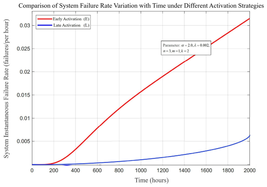
To intuitively demonstrate the suppression effect of the late activation strategy on the system failure rate, Figure 1 presents the curves of the system instantaneous failure rate h(t) over time under different activation strategies with the same Weibull distribution parameters ($\alpha =2.0, \lambda =0.002, n=3, m=1, k=2$).

It can be seen that under the early activation strategy, all spares age synchronously with the main components, leading to a rapid rise in the system failure rate at an early stage; under the late activation strategy, spares are activated with delay, only original components operate initially with a low failure rate, and as original components fail gradually and spares are put into use sequentially, the failure rate rises much more slowly than that under the early activation strategy. This plot verifies the theoretical conclusion in Section 2.4 from the perspective of the failure rate: the late activation strategy yields a lower system failure rate over the entire time domain, thereby achieving higher reliability and a longer mean lifetime.

3. Calculation of Reliability Indices of Cold Standby Systems Under Weibull Distribution

3.1. Analysis of Reliability Index Calculation

Assume that the system has $n$ operating stages, and the lifetime of each stage state is denoted by $T_i(i=1,\cdots ,n)$. The total system lifetime can be expressed as $T_S=T_n+T_{n-1}+\cdots +T_1$. The probability of the system lifetime $T_S$, i.e., system reliability, can be expressed as follows:

$$R_S(t)= P\left(T_S>t\right)=P\left(T_n+T_{n-1}+\cdots T_1>t\right)$$

(17)

For the Weibull distribution, conditional probabilities between various states are required. Equation (17) can be further expanded and analyzed as follows:

$$P\left(T_S>t\right)={\displaystyle {\int }_0^t{f}_{T_1}(t_1)}P\left(T_n+T_{n-1}+\cdots T_2>t-t_1|T_1=t_1\right)\mathrm{d}{t}_1,$$

(18)

where $f_{T_1}(t_1)$ is the probability density function (PDF) of $T_1$, and $P\left(T_n+T_{n-1}+\cdots T_2>t-t_1|T_1=t_1\right)$ is the probability that the sum of the remaining lifetimes is greater than $t-x$, given that $t-x$. According to this method, $P\left(T_S>t\right)$ can be further expressed as follows:

$$P\left(T_S>t\right)={\displaystyle {\int }_0^t{f}_{T_1}(t_1)}\cdot \left[{\displaystyle {\int }_0^{t-t_1}{f}_{T_2|T_1}(t_2|t_1)\cdot }P(T_n+T_{n-1}+\cdots T_3>t-t_1-t_2|T_1=t_1,T_2=t_2)\mathrm{d}{t}_2\right]\mathrm{d}{t}_1$$

(19)

where $f_{T_2|T_1}(t_2|t_1)$ is the PDF of $T_2$ under the condition that $T_1=t_1$ has been fulfilled.

Continuing this recursive process, the system lifetime distribution can be expressed as follows:

$$P\left(T_S>t\right)={\displaystyle {\int }_0^t{\displaystyle {\int }_0^{t-t_1}\cdots }}{\displaystyle {\int }_0^{t-t_1-\cdot \cdot \cdot -t_n}{f}_{T_1}(t_1)}\cdot f_{T_2|T_1}(t_2|t_1)\cdots f_{T_n|T_1,T_2,\cdots ,T_{n-1}}(t_n|t_1,t_2,\cdots t_{n-1})\mathrm{d}{t}_n\cdots \mathrm{d}{t}_2\mathrm{d}{t}_1$$

(20)

This expression clearly demonstrates that the probability of the system lifetime $T_S$ is determined by the PDFs of each state and their conditional probability relationships. However, due to the multi-stage structure, obtaining an analytical expression becomes complex. Therefore, in practical applications, a Markov model is often employed to solve these problems.

3.2. Establishment and Solution of Non-Homogeneous Markov Model

A non-homogeneous Markov model is used to describe time-dependent state transitions. Unlike the standard Markov model, the non-homogeneous Markov model allows the state transition probability to change with time, making it suitable for systems where state transition rules vary over time. For equipment whose lifetime follows the Weibull distribution, the failure rate changes with time, and the non-homogeneous Markov model effectively captures reliability behavior under time-dependent failure rates.

3.2.1. Non-Homogeneous Markov Model

Assume that the system has $n$ possible states and the state space can be expressed as follows:

$$S=\left\{S_1,S_2,\cdots ,S_n\right\}$$

(21)

Each state $S_i$ represents the state of the system at a specific moment.

In the non-homogeneous Markov model, the state transition matrix $P(t,\Delta t)$ is defined as follows:

$$P(t,\Delta t)=\left(\begin{array}{cccc}{p}_{11}(t,\Delta t)& p_{12}(t,\Delta t)& \cdots & p_{1n}(t,\Delta t)\\ p_{21}(t,\Delta t)& p_{22}(t,\Delta t)& \cdots & p_{2n}(t,\Delta t)\\ ⋮& ⋮& \ddots & ⋮\\ p_{n1}(t,\Delta t)& p_{n2}(t,\Delta t)& \cdots & p_{nn}(t,\Delta t)\end{array}\right)$$

(22)

where $p_{ij}(t,\Delta t)$ represents the probability of transitioning from state $S_i$ to state $S_j$ at time $t$ over a time interval $\Delta t$. For any states $S_i$ and $S_j$, $p_{ij}(t,\Delta t)\ge 0$. For each time $t$, ${\displaystyle \sum _{j=1}^n{p}_{ij}(t,\Delta t)}=1$.

Given the initial state $S_i$ and initial time $t_0$, the state probability vector $P_S(t)$ at time $t$ can be obtained recursively using the state transition matrix. If there are a total of $n$ transitions from the initial time $t_0$ to time $t$ with a step size $\Delta t$, then

$$P_S(t)=P\left(t_0+n\Delta t,\Delta t\right)\cdots P(t_0+\Delta t,\Delta t)\cdot P(t_0,\Delta t)\cdot P_S\left(t_0\right)$$

(23)

where $P_S(t)$ is the state probability vector at time $t$ with dimension $n\times 1$. $P(t,\Delta t)$ is the state transition matrix at time $t$ with dimension $n\times n$. $P_S\left(t_0\right)$ is the state probability vector at the initial time $t_0$ with dimension $n\times 1$.

3.2.2. State Analysis of $k/n:m(G)$ Cold Standby Voting System

The $k/n:m(G)$ cold standby voting system consists of $(n-k)+m+2$ states, including $(n-k)+m+1$ states corresponding to normal operation. These states are defined as follows:

$S_0$: All components of the main system are operational, and the cold standby parts are not activated.

$S_i$: $i$ components have failed, but the cold standby parts are not yet activated $1\le i\le n-k$.

$S_i$: $i$ components have failed, and the cold standby parts $i-(n-k)$ are activated, $n-k+1\le i\le n+m-k$.

$S_{n-k+m+1}$: The system has failed.

The probability of the system operating in each state of the cold standby voting system is denoted as $p_{S_i}(t)$, $i=0,1,\cdots ,n-k+m+1$. Therefore, the probability that the system is operating normally at time $t$, i.e., reliability, is as follows:

$$R(t)={\displaystyle \sum _{i=0}^{n-k+m}{p}_{S_i}(t)}$$

(24)

3.2.3. Confirmation of Single Component Transition Probability

The initial state $S_0$ of the cold standby voting system is one where all components of the main system are operational. The transition probability in this state is analyzed as follows:

$$R(t)={\mathrm{e}}^{-{\displaystyle {\int }_0^t\lambda (t)\mathrm{d}t}}$$

(25)

Using the definition of integration, this formula is decomposed further. Assuming that each state transition occurs in steps of size $\Delta t$, the number of steps required to transition from time 0 to $t$ is $t=n\cdot \Delta t$. Then,

$$\begin{array}{ll}R(t)& ={\mathrm{e}}^{-{\displaystyle {\int }_0^t\lambda (t)\mathrm{d}t}}\\ & ={\mathrm{e}}^{-{\displaystyle \sum _{i=0}^n\lambda (i\cdot \Delta t)\cdot \Delta t}}\\ & ={\mathrm{e}}^{-\lambda (0)\cdot \Delta t}\cdot {\mathrm{e}}^{-\lambda (\Delta t)\cdot \Delta t}\cdot {\mathrm{e}}^{-\lambda (2\cdot \Delta t)\cdot \Delta t_1}\cdots {\mathrm{e}}^{-\lambda (n\cdot \Delta t)\cdot \Delta t}\end{array}$$

(26)

Therefore, the probability of a single component in the system transitioning from normal to normal in each step is ${\mathrm{e}}^{-\lambda (i\cdot \Delta t)\cdot \Delta t}$, while the probability of transitioning from normal to failure is $1-{\mathrm{e}}^{-\lambda (i\cdot \Delta t)\cdot \Delta t}$, where $\lambda (t)$ represents the failure rate of the component at time $t$.

Assume that $T=n_1\cdot \Delta t$ and that the probability of the system being in state $S_0$ at time $t$ is $p_{S_1}(n_1\cdot \Delta t)$; then there are $k$ normal components in state $S_0$. The transition probability of components from normal to normal is ${\mathrm{e}}^{-\lambda (n_1\cdot \Delta t)\cdot \Delta t}$. The probability of being in state $S_0$ at time $(n_1+1)\cdot \Delta t$ is $p_{S_1}(n_1\cdot \Delta t)\cdot {({\mathrm{e}}^{-\lambda (n_1\cdot \Delta t)\cdot \Delta t})}^k$.

Since cold standby parts do not degrade before activation, it is necessary to account for the state of the cold standby parts at each step to update their reliability. Consider the following example:

Assume there is only one cold standby part. Initially, when the cold standby part is not activated, its reliability is 1.

After one state transition: Suppose the transition takes time $\Delta t$. The probability of activating the cold standby part at this time is $p$. If activated, the current degradation time of the cold standby part is set to 0, and its reliability remains at 1.

After another state transition: After another time $\Delta t$, the probability of activating the cold standby part is $p$. Compared to the previous state, the reliability of the cold standby part becomes $p\cdot {\mathrm{e}}^{-\lambda (\Delta t)\Delta t}$. If the cold standby part is activated, its reliability is reset to 1. The reliability values at these two moments are recorded as $[p\cdot {\mathrm{e}}^{-\lambda (\Delta t)\Delta t},p]$.

For each additional state transition, the reliability of the cold standby part is recorded as $[p\cdot {\mathrm{e}}^{-\lambda (\Delta t)\Delta t}\cdot {\mathrm{e}}^{-\lambda (2\cdot \Delta t)\Delta t},p\cdot {\mathrm{e}}^{-\lambda (\Delta t)\Delta t},p]$.

Thus, the probability of activating the cold standby part after each transition can be obtained.

3.3. Monte Carlo Simulation

Monte Carlo simulation is a powerful tool for system reliability evaluation. Reference [16] applied this method to analyze cold standby voting systems with exponentially distributed component lifetimes. However, it did not consider the Weibull distribution, which is more relevant in practical engineering applications. To address this limitation, this section extends the approach in Reference [16] to accommodate Weibull-distributed lifetimes.

3.3.1. Sample Setting

Sample size determination is a key step in Monte Carlo simulation. An appropriate sample size improves result accuracy while maintaining computational efficiency. It depends on several factors, including the complexity of the problem, the desired level of accuracy, computational resource constraints, and the distribution characteristics of random variables. To ensure the accurate estimation of the population mean with a specified confidence level, this study determines the minimum required sample size based on the classical formula for sample size calculation, as described in Reference [17]. The formula, derived from the confidence interval of the population mean, is given by the following:

$$N={({\displaystyle \frac{Z_{a/2}\cdot \sigma }{E}})}^2$$

(27)

where $N$ is the required sample size, $Z_{a/2}$ is the value corresponding to the required confidence level (for example, $Z_{a/2}$ = 1.96 for a 95% confidence level), $\sigma$ is the sample standard deviation, and $E$ is the absolute error. The standard deviation can be calculated using the following:

$$\sigma =\sqrt{{\displaystyle \frac{{\displaystyle \sum _{i=1}^n{(x_i-\overline{x})}^2}}{n-1}}}$$

(28)

In actual simulation, based on a 95% confidence level ($Z_{a/2}$ = 1.96), through preliminary experiments, the standard deviations $\sigma$ and absolute error $E$ of the system lifetime under each operating mechanism are estimated. Then the minimum sample size $N$ required for the simulation can be calculated according to Equation (27). In general engineering applications, the required sample size for Monte Carlo simulation is $N\ge {10}^5$.

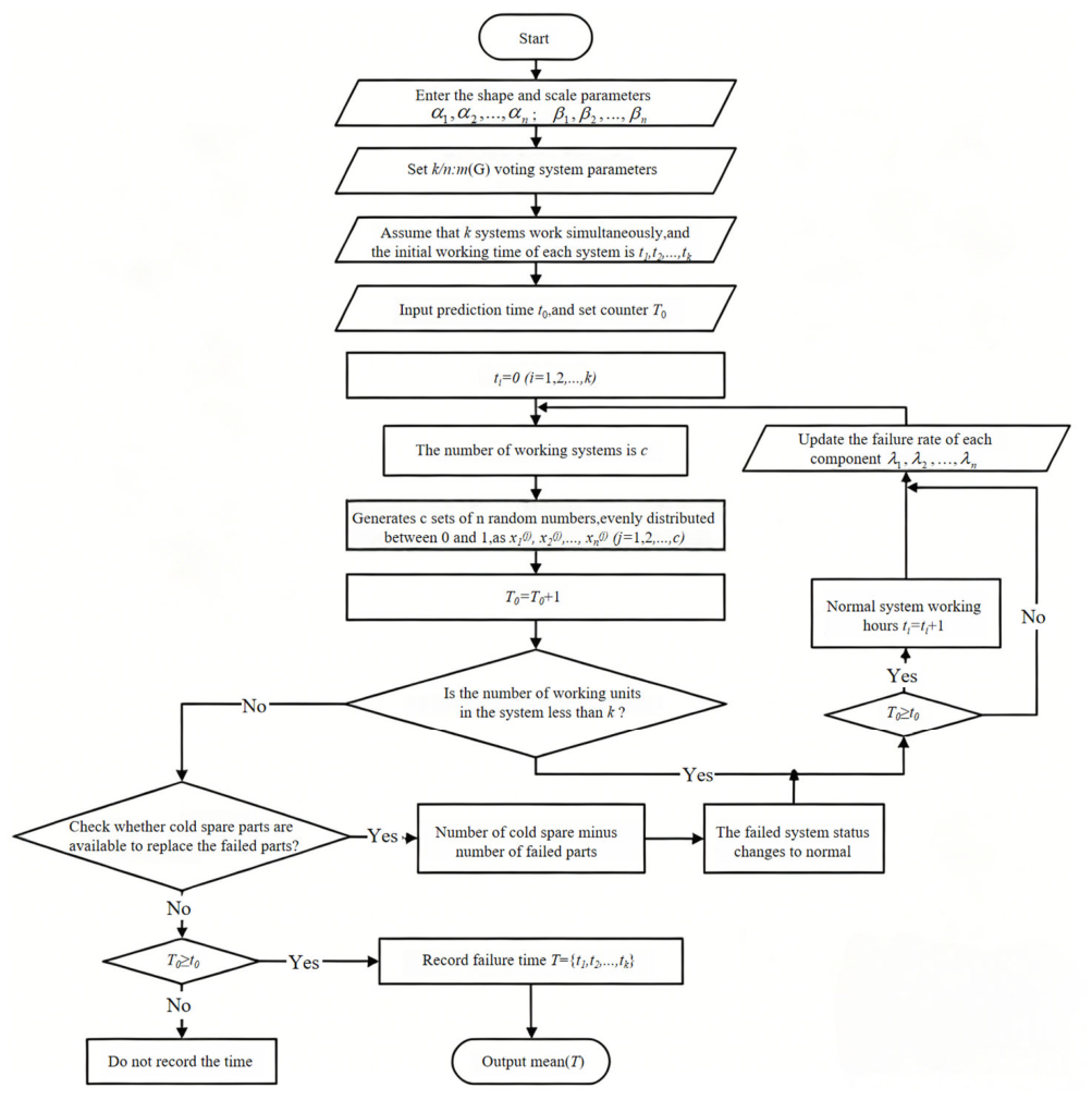
3.3.2. Design of Monte Carlo Simulation Process

This section establishes a remaining useful life prediction model based on Monte Carlo simulation. With the failure rates ${\lambda }_1,{\lambda }_2,\cdots ,{\lambda }_n$ of individual components within the system as inputs, the model simulates the system lifetime process via random sampling and computes reliability indices by statistically analyzing the distribution of system failure times.

Detailed Procedure:

Step 1: Input Parameters

Input the shape parameter ${\alpha }_1,{\alpha }_2,\cdots ,{\alpha }_n$ and scale parameter ${\beta }_1,{\beta }_2,\cdots ,{\beta }_n$.

Set the number of operating components of the $k/n:m(G)$ voting system to $n$, voting threshold $k$, and the number of cold standby components $m$.

Assume that $k$ systems operate simultaneously with an initial operating time $t_1,t_2,\cdots ,t_k$ of 0.

Input the prediction time $t_0$, and initialize the counter $T_0=0$.

Step 2: Simulation Loop

(1) Determine the number of operating components: Obtain the current count $c$ of normally functioning components in the system.

(2) Generate $n$ uniform random numbers $x_1^{(j)},x_2^{(j)},\cdots ,x_n^{(j)}$ over $\left[0,1\right]$ for each normal system to determine component failures.

(3) Increment the time step, $T_0=T_0+1$.

(4) Judge whether each system is functioning normally (i.e., the number of operating units is less than $k$):

System failure: Initiate the failure recording routine. Check whether cold spare parts are available to replace the failed components.

If no spare parts are available, the system ultimately fails due to insufficient spare support.

If spare parts are available, activate the cold standby component, reset its service life to 0 upon deployment, maintain normal system status, and proceed to the next iteration.

System normal: Continue inspecting spare status, update component failure rates ${\lambda }_1,{\lambda }_2,\cdots ,{\lambda }_n$, and accumulate the operating time $t_i=t_i+1$ of normal systems.

(5) For failed systems that are repaired, set their status to normal.

Step 3: Output Results

Record the set of failure times $T=\left\{t_1,t_2,\cdots ,t_k\right\}$ for all systems, and output the mean value $mean\left(T\right)$ of $T$.

The algorithm flow is shown in Figure 2.

4. Example Simulation

In railway signal systems, the stable operation of signal control equipment is critical to train safety and efficiency. To adapt to complex operating conditions and potential failures, such systems typically adopt a multi-device collaborative working mode. This involves series, parallel, and $k/n(G)$ voting configurations, along with backup equipment to facilitate rapid fault replacement. This design enables continuous and stable system operation.

Assume that the main system consists of three signal control devices, denoted as $S_1$, $S_2$, and $S_3$ with one standby signal control device $S_b$ available. The failure time $T_{S_i}~W(\alpha ,\beta )$ of each signal control device follows a Weibull distribution.

Based on varying reliability requirements, the system is designed with three core operating mechanisms, described as follows. (1) G1: 3/3:1(G)—The system operates normally only if all three main control devices are functional, following a series-type logic with high reliability demands. (2) G2: 1/3:1(G)—The system remains operational if at least one of the three main control devices is functioning, following a parallel-type logic that emphasizes continuity. (3) G3: 2/3:1(G)—The system operates normally if at least two of the three main control devices are functioning, embodying a voting-type logic that balances reliability and fault tolerance. The standby equipment is deployed to replace any failed device in the main system immediately.

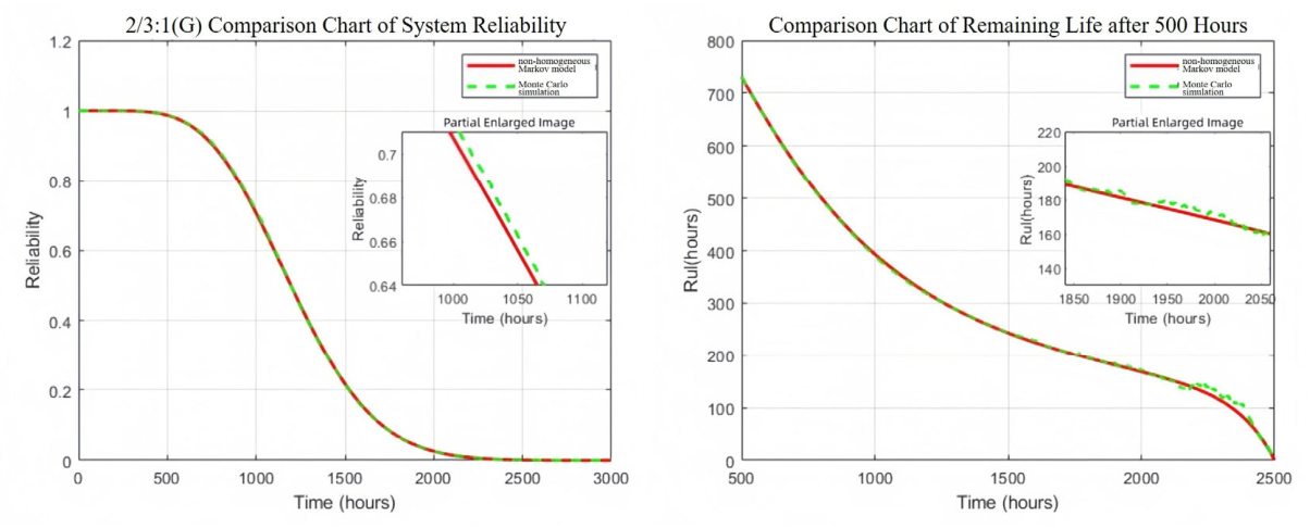
Given the parameters $T_{S_i}~W(\alpha ,\beta )$, $\alpha =2$, and $\beta =1000$, in this simulation, the preliminary experiment yielded a sample standard deviation of $\sigma \approx 254 \mathrm{h}$ and an absolute error of $E\approx 1.28 \mathrm{h}$. Calculated according to Equation (27) and rounded off, the result is $N=\mathrm{155,551}$, which satisfies the requirement of $N\ge {10}^5$, so it is applicable. The simulation step size is taken as $\Delta t=0.1 \mathrm{h}$. The operational performance of the system under these different working mechanisms is accurately evaluated using both the non-homogeneous Markov model and the Monte Carlo simulation model. These models are employed to predict and analyze the system’s average life, remaining life after 500 h of operation, and overall reliability. The prediction results of both models are compared and presented through data comparison and graphical visualization.

The comparison of prediction values and prediction rates for different remaining life prediction models, based on the non-homogeneous Markov and Monte Carlo simulation models, is summarized in

Table 1. Comparison table of remaining life prediction (hour) with 95% confidence interval (CI) and standard deviation (Std).

System Work Program	G1: 3/3:1(G)	G2: 1/3:1(G)	G3: 2/3:1(G)
Non-homogeneous Markov model (Mean, 95%CI, Std)	401.28, [392.15, 410.41], 12.36	1532.42, [1518.12, 1546.72], 20.41	732.41, [723.58, 741.24], 9.87
Monte Carlo simulation model (Mean, 95%CI, Std)	391.11, [382.34, 399.88], 11.87	1552.33, [1537.24, 1567.42], 21.05	726.51, [717.93, 735.09], 9.62
Deviation (%)	2.53	1.30	0.81

and

Table 2. Comparison table of prediction rates of different remaining life prediction (second).

System Work Program	G1:3/3:1(G)	G2:1/3:1(G)	G3:2/3:1(G)
Non-homogeneous Markov model	0.1211	0.1145	0.1101
Monte Carlo simulation model	60.7956	90.8532	105.1369
Time increment ratio (%)	99.80	99.87	99.90

.

Table 1 demonstrates that the predictions of both models are highly consistent, with deviation rates remaining low (≤2.54%). This suggests that the non-homogeneous Markov model offers prediction accuracy comparable to the traditional Monte Carlo simulation model. Notably, the deviation rate under the G3 (2/3:1(G)) mechanism is the lowest (0.8052%), highlighting that the non-homogeneous Markov model delivers the highest prediction accuracy under this operational configuration.

Table 2 demonstrates that the running time of the non-homogeneous Markov model is extremely short, consistently staying below 0.13 s. In contrast, the Monte Carlo model requires significantly more time, ranging from 60 to 105 s, highlighting a substantial disparity between the two. The time cost increase rate for the Monte Carlo model relative to the non-homogeneous Markov model exceeds 99.8%, meaning that the Monte Carlo model demands hundreds of times more time for the same prediction task.

Further analysis reveals that the Monte Carlo model becomes increasingly time-consuming as the system’s working mechanism places greater demands on device collaboration. In contrast, the running time of the non-homogeneous Markov model remains relatively stable or even slightly decreases. This suggests that the non-homogeneous Markov model exhibits superior adaptability under more complex operational configurations and offers a clear efficiency advantage. Meanwhile, the computational complexity of the Monte Carlo model grows substantially with increasing system complexity, leading to a significant rise in running time.

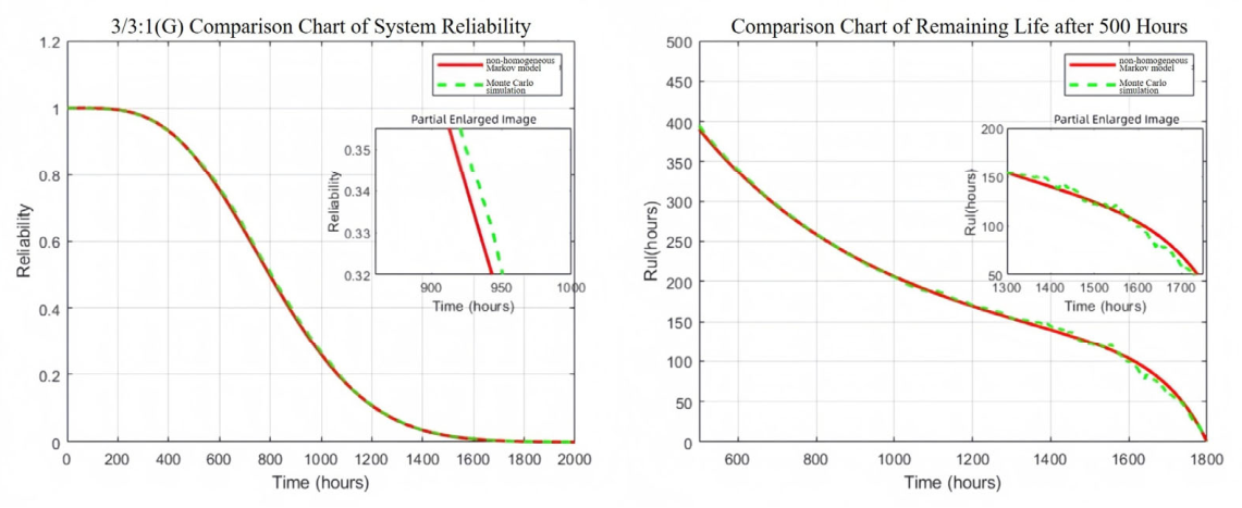
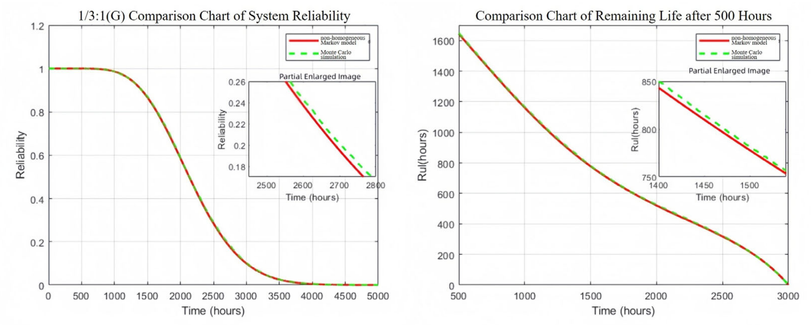
The reliability and remaining life prediction results obtained from both the non-homogeneous Markov model and the Monte Carlo simulation under the three mechanisms, G1, G2, and G3, are presented in Figure 3, Figure 4 and Figure 5, respectively.

For the G1 (3/3:1(G)) mechanism, reliability declines the most rapidly, with a sharp decrease in the early stage (0–1000 h) and stabilization at a low level thereafter. This behavior is attributed to the series configuration, where all units must remain operational; the failure of any single unit leads to a significant reduction in reliability. The remaining life after 500 h is relatively short, ranging from approximately 300 to 400 h. It also exhibits a rapid decay rate. These results indicate a substantially increased failure risk after prolonged operation under the series configuration.

For the G2 (1/3:1(G)) mechanism, reliability decreases at the slowest rate, remaining at a relatively high level throughout the 5000 h observation period. This behavior reflects the strong fault tolerance of the parallel configuration, where system operation can be sustained even if multiple main devices fail. The remaining life after 500 h is the longest, exceeding 1400 h, and exhibits a gradual decay over time. These results indicate that the parallel mechanism maintains stable performance even after prolonged operation.

For the G3 (2/3:1(G)) mechanism, the reliability decline rate lies between those of the G1 and G2 mechanisms. It remains relatively stable in the early stage and gradually decreases in the later stage. This behavior is consistent with the design principle of the 2/3 voting mechanism, which avoids the high failure risk of the G1 configuration while reducing excessive dependence on a single device, thereby achieving a balance between reliability and fault tolerance. The remaining life after 500 h is approximately 700–800 h and exhibits a moderate decay rate, reflecting the typical lifetime characteristics of voting systems.

Under all three operating mechanisms, the reliability trends predicted by the non-homogeneous Markov model (state transition method) and the Monte Carlo method show a high degree of agreement. The predicted curves of remaining life after 500 h are also closely aligned. This consistency confirms the accuracy of the non-homogeneous Markov model. As shown in Figure 3, Figure 4 and Figure 5, the results of both methods remain highly consistent during key intervals where reliability changes either rapidly or gradually, with no significant deviations observed. These results demonstrate that the non-homogeneous Markov model accurately captures reliability variations and maintains strong predictive stability.

Overall, when component and spare part lifetimes follow the Weibull distribution, the parallel mechanism provides the highest fault tolerance and longest lifetime, whereas the series mechanism imposes the strictest reliability requirements and yields the shortest lifetime. The voting mechanism offers a balanced compromise between these two, allowing for the selection of an appropriate configuration based on practical engineering needs. The non-homogeneous Markov model effectively supports the high-accuracy prediction of residual life and system reliability in cold standby voting systems. Compared with Monte Carlo simulation, it significantly reduces computational cost, with its efficiency advantage becoming more pronounced under complex configurations (e.g., G3), making it suitable for fast engineering prediction.

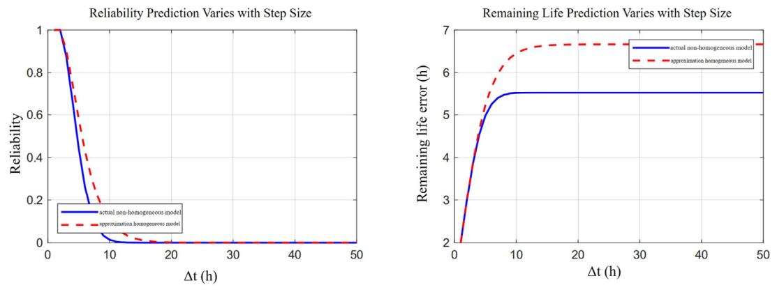
Considering the reliability time scales of typical engineering systems (such as electromechanical and aerospace electronic systems), when the abscissa time (hours) spans from hundreds to thousands of hours, the commonly used step size ranges from 0.1 to 1 h. Therefore, a step size of 0.1 h is adopted in this simulation.

However, in practical scenarios, the prediction accuracy of the non-homogeneous Markov model is related to the prediction step size. Sensitivity comparison charts for different step sizes are shown in Figure 6. In future research, the stability and practicability of the model can be further improved by optimizing the step size adaptive algorithm.

5. Conclusions

This study proves that delayed activation maximizes the system mean lifetime. To address the difficulty of obtaining analytical solutions for reliability indices under the Weibull distribution, a non-homogeneous Markov model is developed, as well as corresponding reliability evaluation procedures. This approach enables the efficient computation of both mean lifetime and residual life. The results show strong agreement with classical Monte Carlo simulations, achieving high accuracy while significantly reducing computational cost.

The proposed model and computational method have strong engineering applicability and can be extended to practical voting systems, such as those used in power equipment and aerospace engineering. The parameters of the Weibull distribution can be estimated from historical data, enabling the accurate prediction of residual life and failure risk and supporting condition-based maintenance decisions.

Future work will focus on extending the proposed approach to network systems. In particular, cold standby redundancy will be incorporated into network reliability optimization, and a reliability evaluation framework for cold standby network systems will be developed. This is expected to provide efficient and practical solutions for network reliability assessment.

References

1. Liu, L.; Ai, X.; Zheng, X. Research on fault localization methods of shipboard power networks. In Proceedings of the Eighth International Conference on Energy System, Electricity, and Power (ESEP 2023), Wuhan, China, 24–26 November 2023; Volume 13159, pp. 1931–1936. [Google Scholar]
2. Wang, H.; Liu, H.; Shao, S. Improved bootstrap method based on RBF neural network for reliability assessment. Appl. Sci. 2024, 14, 2901. [Google Scholar] [CrossRef] [Scilit]
3. Wang, H.; Liu, H.; Shao, S.; Zhang, Z. Methodology of shipboard spare parts requirements based on whole part repair strategy. Mathematics 2024, 12, 3053. [Google Scholar] [CrossRef] [Scilit]
4. Yang, L.; Zhang, X.; Lu, Z.; Fu, Y.; Moens, D.; Beer, M. Reliability evaluation of a multi-state system with dependent components and imprecise parameters: A structural reliability treatment. Reliab. Eng. Syst. Saf. 2024, 250, 110240. [Google Scholar] [CrossRef] [Scilit]
5. Zong, X.; Liu, Z.; Li, C. Reliability analysis of single cold standby k/n voting system. In Proceedings of the Aerospace Reliability Academic Exchange Conference, Beijing, China, 31 August 2013; pp. 620–625. [Google Scholar]
6. Hu, T.; Sun, Y.; Li, X. Reliability solution of cold standby voting systems with arbitrary distributions. Syst. Eng. Electron. 2022, 44, 2357–2363. [Google Scholar]
7. Gu, R. Research on Reliability Analysis and Evaluation Methods of Common Load Failure Systems. Master’s Thesis, Beihang University, Beijing, China, 2013. (In Chinese) [Google Scholar]
8. Franko, C.; Tutuncu, G.Y.; Eryilmaz, S. Reliability of weighted k-out-of-n: G systems consisting of two types of components and a cold standby component. Commun. Stat. Simul. Comput. 2017, 46, 4067–4081. [Google Scholar] [CrossRef] [Scilit]
9. Zhu, Q. Reliability analysis of voting systems with cold standby units. Electron. Prod. Reliab. Environ. Test. 2006, 3, 32–35. [Google Scholar]
10. Roy, A.; Gupta, N. Reliability function of k-out-of-n system equipped with two cold standby components. Commun. Stat. Theory Methods 2021, 50, 5759–5778. [Google Scholar] [CrossRef] [Scilit]
11. Eryilmaz, S. On the mean residual life of a k-out-of-n: G system with a single cold standby component. Eur. J. Oper. Res. 2012, 222, 273–277. [Google Scholar] [CrossRef] [Scilit]
12. Dembińska, A.; Nikolov, N.; Stoimenova, E. Reliability properties of k-out-of-n systems with one cold standby unit. J. Comput. Appl. Math. 2021, 388, 113289. [Google Scholar] [CrossRef] [Scilit]
13. Ioannis, S. Combined m-Consecutive-k-out-of-n: F and Consecutive kc-out-of-n: F Structures with cold standby redundancy. Mathematics 2023, 11, 2597. [Google Scholar]
14. Eryilmaz, S. A study on reliability of coherent systems equipped with a cold standby component. Metrika 2014, 77, 349–359. [Google Scholar] [CrossRef] [Scilit]
15. Zhang, B.; Hu, C.; Zheng, J.; Pei, H. Maintenance decision-making using intelligent prognostics within a single spare parts support system. Sensors 2025, 25, 837. [Google Scholar] [CrossRef] [Scilit] [PubMed]
16. Liu, L.; Ai, X.; Wu, J. Reliability and residual life of cold standby systems. Mathematics 2024, 12, 1540. [Google Scholar] [CrossRef] [Scilit]
17. Cochran, W.G. Sampling Techniques, 3rd ed.; John Wiley & Sons: New York, NY, USA, 1977. [Google Scholar]
Figure 1. Comparison of system failure rate over time between late activation and early activation strategies.
Mathematics 14 01533 g001
Figure 2. Residual life prediction model under Weibull distribution (Monte Carlo simulation).
Mathematics 14 01533 g002
Figure 3. A 3/3:1 (G) comparison chart of system reliability and remaining life prediction.
Mathematics 14 01533 g003
Figure 4. A 1/3:1 (G) comparison chart of system reliability and remaining life prediction.
Mathematics 14 01533 g004
Figure 5. A 2/3:1 (G) comparison chart of system reliability and remaining life prediction.
Mathematics 14 01533 g005
Figure 6. Influence of step size on prediction accuracy of non-homogeneous Markov models (2/3:1(G)).
Mathematics 14 01533 g006