Article

Efficient Calibration for Option Pricing via a Physics-Informed Chebyshev Kolmogorov–Arnold Network


1
School of Science, Xi’an University of Posts and Telecommunications, Xi’an 710121, China
2
School of Computer Science and Technology, Xi’an University of Posts and Telecommunications, Xi’an 710121, China
3
School of Information Communication Engineering, Beijing Information Science and Technology University, Beijing 102206, China
*
Authors to whom correspondence should be addressed.
Mathematics 2026, 14(9), 1529; https://doi.org/10.3390/math14091529
Submission received: 6 March 2026 / Revised: 5 April 2026 / Accepted: 7 April 2026 / Published: 30 April 2026
(This article belongs to the Section E5: Financial Mathematics)

Abstract

Efficient calibration is essential for the practical application of option pricing models. The Fractional Stochastic Volatility Jump Diffusion (FVSJ) model can reproduce several stylized features observed in option markets, including the volatility smile, volatility clustering, and long-memory effects. However, its multiple stochastic components make conventional calibration computationally expensive. This paper proposes a two-step calibration framework that combines a neural network with a differential evolution (DE) algorithm. In the first step, we construct a Physics-Informed Kolmogorov–Arnold Network (PCKAN) to approximate the FVSJ pricing map. Specifically, we replace the B-spline basis in KAN with second-kind Chebyshev polynomials and incorporate a Black–Scholes PDE residual as an additional penalty term in the training objective, aiming to improve global approximation and enhance numerical stability and interpretability. In the second step, the trained PCKAN is used as a fast surrogate pricer within the DE algorithm to accelerate parameter estimation. Empirical results show that the proposed method achieves calibration accuracy comparable to direct pricing while substantially reducing computational time.

1. Introduction

Model calibration aligns option pricing models with observed market data by minimizing discrepancies between theoretical assumptions and empirical behavior. It is therefore essential for practical derivative valuation as well as for providing quantitative inputs to risk measurement and hedging. Although the Black–Scholes (BS) model [1] remains widely used due to its analytical tractability, it does not adequately reproduce key stylized market features, including volatility smiles, volatility clustering, jumps, and long-memory effects [2,3,4,5,6,7,8]. To address these limitations, Zhang, Yong, and Xiao [9] proposed the Fractional Stochastic Volatility Jump Diffusion (FVSJ) model, which combines Heston-type stochastic volatility with fractional volatility dynamics and a mixed exponential jump diffusion component [10,11,12,13,14,15,16,17,18,19,20,21]. Notably, Zhang and Sun [22] had previously conducted foundational research on option pricing with double stochastic volatility, stochastic interest rates, and double jumps, providing valuable theoretical support for the development of the FVSJ model. However, the increased model complexity and high-dimensional parameterization make calibration in practice computationally intensive and may reduce numerical stability.
Traditional model calibration methods are generally classified into two categories: statistical inference and error minimization. In the statistical inference framework, Lin et al. [23] used maximum likelihood estimation to optimize the free parameters of latent Gaussian models. Mulenga et al. [24] adopted a Bayesian approach to infer the posterior distribution of time-varying calibrated parameters by combining priors on BS model parameters with observed underlying asset and option data. In practice, inference-based methods often rely on an analytically tractable likelihood or distributional representation of the model, which can be difficult to obtain for complex settings. In the error-minimization paradigm, Hilliard et al. [25] employed weighted nonlinear least squares to estimate parameters of jump diffusion models; Bukh et al. [26] proposed an error-minimization algorithm with an adaptive adjustment rate for parameter fitting; and Gao et al. [27] applied a Gauss–Chebyshev approximation for parameter estimation. These approaches are typically formulated as nonconvex optimization problems and may therefore be sensitive to initialization, increasing the risk of convergence to local minima.
Modern deep-learning-based calibration methods are commonly categorized into one-step and two-step approaches. One-step methods seek to learn the mapping from implied volatility surfaces or market prices to model parameters directly; for example, Joseph et al. [28] calibrated local volatility and stochastic short-rate models using stock call option and interest rate cap prices, and Shi et al. [29] used SPX option prices as calibration targets. Two-step methods first train a neural network surrogate for forward mapping from parameters to prices or implied volatilities and then recover parameters via classical optimization or inference; Büchel et al. [30] approximated Trolle–Schwartz prices with a multilayer perceptron(MLP) and global optimization, while Dadah [31], Horvath et al. [32], and Gazzani et al. [33] learned mappings from parameters and yield curves to implied volatilities and performed inverse calibration. Compared with one-step methods, two-step methods often provide more stable calibration and retain a clearer structural interpretation of parameters. However, their performance still depends on the surrogate’s approximation quality and architecture, and many implementations do not explicitly enforce no-arbitrage conditions, which can lead to economically inconsistent outputs and motivates further methodological refinement.
The Kolmogorov–Arnold Network (KAN) [34] provides an alternative to the multilayer perceptrons commonly used in deep-learning-based calibration and is well suited to function approximation. To further improve its global approximation accuracy, we replace the original B-spline basis functions with second-kind Chebyshev polynomials. To address the lack of explicit financial constraints in many surrogate models, we embed the BS PDE as a regularization term into the loss function, thereby improving the interpretability of the neural network. Building on the two-step calibration paradigm, we integrate the Chebyshev-based KAN with physical information and propose a Physics-informed Chebyshev KAN (PCKAN). In implementation, PCKAN is first trained as a surrogate for the FVSJ pricing function, and model parameters are then calibrated via the differential evolution algorithm.
The main contributions of this paper are twofold. Firstly, this paper proposes a new physics-informed neural network. Secondly, this paper proposes a new two-step calibration algorithm based on the new physics-informed neural network. The rest of the paper is organized as follows. Section 2 presents the model and calibration problem. Section 3 details the calibration algorithm. Section 4 presents some empirical experiments. Section 5 concludes the study.

2. Model Calibration

2.1. FVSJ Model

Let Ω , F , F t 0 t T , denote a complete probability space, where the filtration F t 0 t T satisfies the right-continuity property, and denotes the risk-neutral measure. Within the framework of the Fractional Stochastic Volatility Jump Diffusion model [9], the evolutionary dynamics of the asset price process P t are characterized by the following system of Equation (1):
d P t P t = ( r λ δ ) d t + v 1 t d B 1 t P + v 2 t d B 2 t P + d k = 1 N t ( ζ k 1 ) , d v 1 t = k 1 θ 1 v 1 t d t + σ 1 v 1 t d F 1 t H 1 , d v 2 t = k 2 θ 2 v 2 t d t + σ 2 v 2 t d F 2 t H 2 .
where B 1 t P and B 2 t P are standard Brownian motions, F 1 t H 1 and F 2 t H 1 are fractional Brownian motions with Hurst parameters H 1 and H 2 , respectively, and N t is a Poisson process with intensity λ . Let { Z i } be a sequence of independent and identically distributed non-negative random variables such that Y = ln ς follows a mixed exponential distribution with probability density function:
f Z ( z ) = α k = 1 m α k μ k e μ k z I z 0 + β j = 1 n β j θ ^ j e θ ^ j z I z < 0 ,
where μ k > 1 , θ ^ j > 0 , α 0 , β = 1 α 0 , α k , β j ( , ) , k = 1 m α k = 1 , j = 1 n β j = 1 . To ensure f Z ( z ) is a probability density function, a simple sufficient condition is k = 1 M α k β k 0   ( M = 1 , , m ) , j = 1 L β j θ ^ j 0   ( L = 1 , , n ) , and the necessary conditions are α 1 > 0 , β 1 > 0 , k = 1 m α k η k 0 , j = 1 n β j θ ^ j 0 .
According to Zhang [9] and Thao [35], model (1) can be approximated by the following classical stochastic partial integro-differential equation system:
d S t ε 1 , ε 2 S t ε 1 , ε 2 = ( r λ δ ) d t + v 1 t d W 1 t S + v 2 t d W 2 t S + d k = 1 N t ( ζ k 1 ) , d v 1 t ε 1 = ( H 1 1 / 2 ) ψ 1 t σ 1 v 1 t ε 1 + k 1 θ 1 v 1 t ε 1 d t + ε 1 H 1 1 / 2 σ 1 v 1 t ε 1 d W 1 t v , d v 2 t ε 2 = ( H 2 1 / 2 ) ψ 2 t σ 2 v 2 t ε 2 + k 2 θ 2 v 2 t ε 2 d t + ε 2 H 2 1 / 2 σ 2 v 2 t ε 2 d W 2 t v .
Equation (3) is hereafter denoted as the Fractional Stochastic Volatility Jump Diffusion model (the FVSJ model).
Remark: When λ = 0 , k 2 = 0 , θ 2 = 0 , σ 2 = 0 , H 1 = 1 2 and H 2 = 1 2 , model (1) reduces to the Heston model.
According to [10], the price of a European put option is approximated as follows:
V T 2 n m e r T K k = 0 N 1 ϕ k π n m e i k π m n m U k ,
where
U k = 1 1 + k π ( n m ) 2 k π n m sin m k π n m cos m k π n m + e m + m n k π sin m k π n m ,   k 0 e m m 1 , k = 0 , ϕ ( u ) = exp A ( u ) + B ( u ) + C ( u ) + D ( u ) , A ( u ) = i u ln S 0 K + i u r T ,
B ( u ) = j = 1 2 κ j γ j κ j θ j T Δ j 2 i u ρ j κ j θ j T Δ j + 2 κ j θ j Δ j 2 ln 2 γ j 2 γ j + κ j γ j i u ρ j Δ j 1 e γ j T , C ( u ) = j = 1 2 i u ( i u 1 ) 1 e γ j T 2 γ j + κ j γ j i u ρ j Δ j 1 e γ j T V j ε j ,
D ( u ) = λ T p u i = 1 m p i η i 1 η i i u + q d j = 1 n q j θ ^ j 1 θ ^ j + i u 1 i u δ ,
γ j = κ j i u ρ j Δ j 2 + i u ( 1 i u ) Δ j 2 , Δ j = ε j H j 1 / 2 σ j , δ = p u i = 1 m p i η i 1 η i 1 + q d j = 1 n q j θ ^ j 1 θ ^ j + 1 1 .
K denotes the strike price, T denotes the time to maturity, and r denotes the risk-free interest rate.
According to [36], the integration interval [ c 1 , c 2 ] is defined as follows:
[ m , n ] = c 1 L c 2 , c 1 + L c 2 ,
where L is a truncation coefficient,
c 1 = ln S 0 K 0 + j = 1 2 α j U j 2 k j 1 e m j τ + τ r α 1 + α 2 2 + μ a u i = 1 m a i ξ i b d j = 1 n b j α ^ j a u i = 1 m a i ξ i 1 ξ i 1 + b d j = 1 n b j α ^ j 1 α ^ j + 1 1 , c 2 = μ τ a u i = 1 m 2 a i ξ i 2 + b d j = 1 n 2 b j α ^ j 2 + j = 1 2 Ω 0 j + Ω 1 j e m j τ + Ω 2 j e 2 m j τ ,
Π 0 j = α j τ + 1 m j ( α j + U j α j Δ j ρ j τ ) + 1 m j 2 Δ j ρ j ( 2 α j U j ) + 1 4 α j Δ j 2 τ Δ j 2 8 m j 3 ( 5 α j 2 U j ) , Π 1 j = Δ j ρ j m j 2 ( U j 2 α j ) + 1 m j ( 1 Δ j ρ j τ ) ( α j U j ) + α j Δ j 2 2 m j 3 + τ Δ j 2 ( α j U j ) 2 m j 2 , Π 2 j = Δ j 2 8 m j 3 ( α j 2 U j ) , Δ j = ε j G j 1 / 2 σ j .

2.2. Model Calibration Problem

From an error-minimization perspective, calibration is formulated as an optimization problem. Using observed market prices of European put options together with observable inputs (e.g., strike, risk-free rate, time to maturity, and the underlying price), we calibrate the FVSJ model by estimating its parameter vector. Given a set of model parameters β and option data O , the calibrated parameters are obtained by solving
arg   min   P F V S J ( O , β ) ,
where F V S J ( O , β ) is the theoretical option price computed from Equation (4) and P denotes the market price. The objective minimizes the pricing error between them across the available option quotes.
In practice, solving optimization (6) can be computationally expensive because the iterative search requires repeated evaluations of the FVSJ pricing function. To reduce this burden and improve numerical stability, we employ a neural network as a surrogate pricing function and reformulate (6) as an optimization problem based on the network-predicted option price:
arg   min   P N N ( O , β ) ,
where N N ( O , β ) denotes the predicted price produced by the neural network. Through pre-training, the neural network is trained to approximate the theoretical price calculated by Equation (4). It can then rapidly process parameter inputs during subsequent calibration, thereby enhancing calibration efficiency.

3. Calibration Algorithm

3.1. PCKAN Neural Network

KAN is a neural network architecture based on the Kolmogorov–Arnold representation theorem. According to [34], most multivariate continuous functions f x 1 , x 2 x n can be expressed as a combination of a finite number of univariate continuous functions as follows
f ( x ) = f ( x 1 , , x n ) = q = 0 2 n Φ q p = 1 n φ q , p ( x p ) ,
where Φ q and φ q , p are univariate functions. KAN operationalizes this idea by placing learnable univariate functions on network edges: before being aggregated in the next layer, each input channel is transformed by individual univariate mapping. By contrast, an MLP applies a shared, fixed activation function to its neurons. Accordingly, the layer mappings of KAN and MLP can be written in the simplified forms
M L P ( x ) = ( W L σ W L 1 σ W 1 σ W 0 σ ) ,
K A N ( x ) = ( Φ L Φ L 1 Φ 1 Φ 0 ) ,
where σ denotes the activation function and Φ i denotes a learnable univariate function. In practice, each univariate function Φ i is parameterized by a basis expansion, for example,
Φ ( x ) = i c i B i ( x ) ,
where c i represents learnable coefficients and B i ( x ) denotes B-spline basis functions defined on a grid.
In option pricing and calibration, inputs are often high-dimensional and large-scale, making the B-spline parameterization in KAN computationally expensive and potentially prone to overfitting. Its local support may also limit the capture of global structure. To address these issues, we replace B-splines with second-kind Chebyshev polynomials, which provide a globally defined orthogonal basis with efficient recurrence relations, stable evaluation, and straightforward tensor-product extensions to higher dimensions. With this modification, we obtain the Chebyshev Kolmogorov–Arnold Network (CKAN). The recurrence relation of the second-kind Chebyshev polynomials is given in Equation (12):
U 0 ( x ) = 1 , U 1 ( x ) = 2 x , U n + 1 ( x ) = 2 x U n ( x ) U n 1 ( x ) ( n 1 ) .
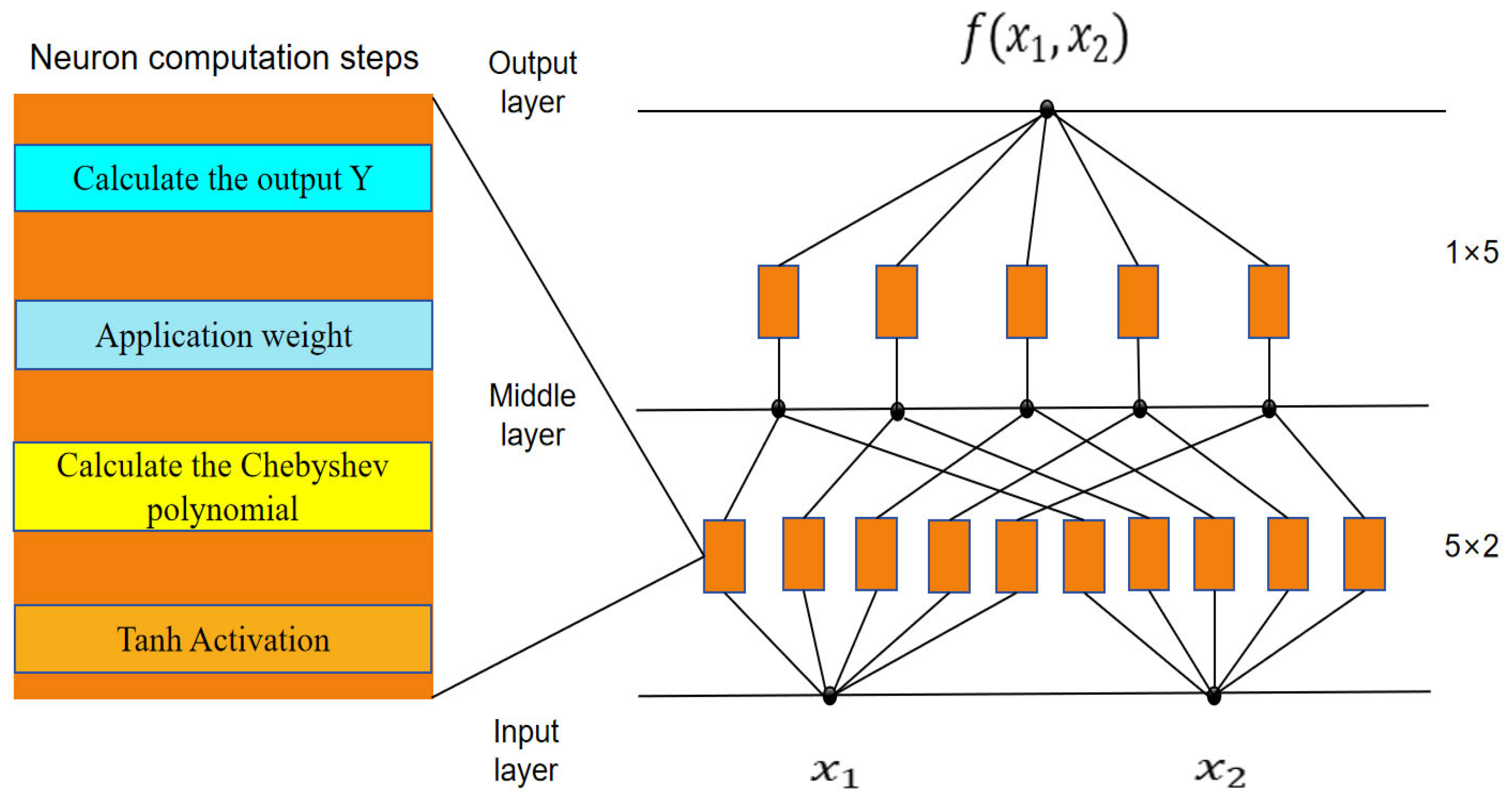
CKAN retains the same overall architecture as KAN, but replaces the basis representation used within each univariate edge function. A two-layer CKAN is illustrated in Figure 1.
As illustrated in Figure 1, CKAN applies Tanh ( · ) normalization to map inputs to [−1, 1], expands them using second-kind Chebyshev polynomials, and then aggregates the resulting features through learnable weights. Specifically, the computation follows Equations (13)–(17):
X tanh = Tanh ( X ) ,
U 0 = 1 , U 1 = 2 X Tanh , U n + 1 = 2 X Tanh U n U n 1 ( n 1 ) ,
C = s t a c k [ U 0 , U 1 , U n ] ,
S = n = 0 D l C n W n ,
Y = S W .
These steps can be compactly written as follows:
Y = p = 1 n 1 W q , p n = 0 D l W q , p , n U n ( X p ) .
Equation (18) shows that CKAN employs two sets of parameters: W q , p for linear feature mixing, W q , p for weighting the polynomial expansion and D l for the highest expansion order of Chebyshev polynomials. This decoupling provides separate control over linear and nonlinear components, improving modeling flexibility.
Although CKAN improves the basis representation in KAN, it remains data-driven and does not explicitly enforce option-pricing structure (e.g., no-arbitrage and pricing dynamics), which limits financial interpretability. We therefore incorporate the BS PDE [2] as a physics-informed constraint. The BS PDE characterizes the price dynamics with respect to the underlying asset price and time to maturity and provides a standard theoretical foundation for option pricing. Specifically, we embed the BS PDE into the CKAN loss function to obtain the proposed PCKAN model. The BS PDE is given in Equation (19).
P t + r S P S + 1 2 σ 2 S 2 2 P S 2 r P = 0 ,
where P denotes the option price, t denotes the time to maturity, r is the risk-free interest rate, S denotes the underlying asset price, and σ denotes the volatility of the underlying asset price.
The loss function L p h y s of PCKAN is defined in Equation (20):
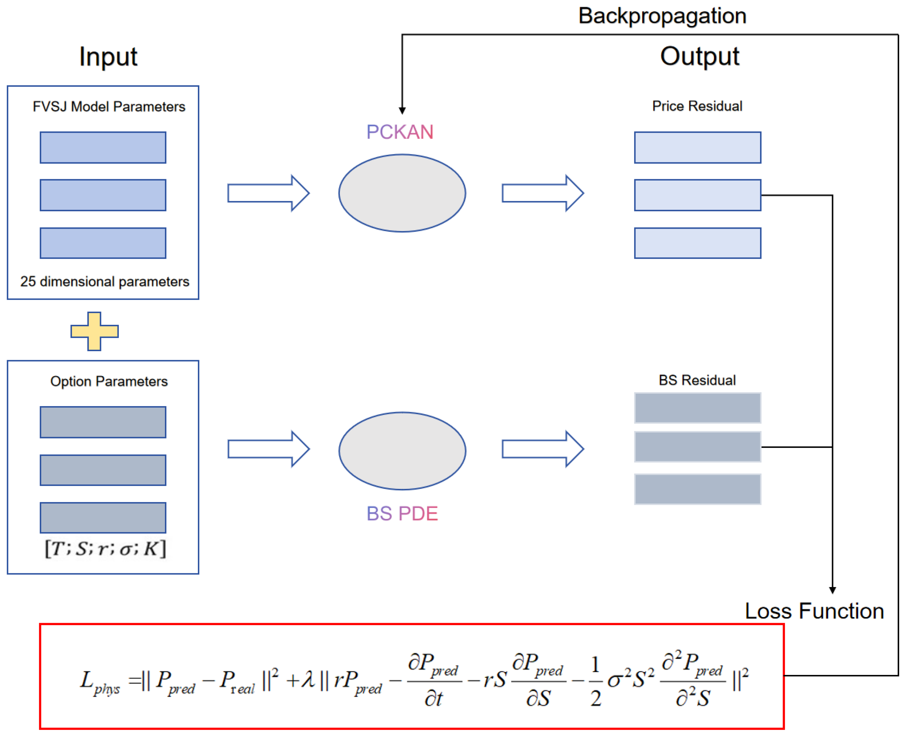
L p h y s = P p r e d P r e a l 2 + λ r P p r e d P p r e d t r S P p r e d S 1 2 σ 2 S 2 2 P p r e d 2 S 2 .
The PCKAN loss is defined in (20) as the sum of a data-misfit term and a physics-informed term. The first term measures the discrepancy between the predicted option price P p r e d and the observed price P r e a l , while the second penalizes the BS PDE residual, where a fixed weighted hyperparameter λ = 0.1 is used to balance the relative contributions of the two loss components. This weighting setting follows the widely accepted paradigm in the application of Physical Informed Neural Networks (PINN) for option pricing [37], which validates that moderate PDE penalty weights can effectively standardize model training without distorting the pricing features of the underlying stochastic model. The data flow of PCKAN is shown in Figure 2.
During training, the loss combines a data-misfit term (between the network-predicted and observed option prices) with a physics term that penalizes the BS PDE residual. The PDE residual is computed via automatic differentiation and evaluated alongside the forward pass, enabling parallel execution and reducing the additional overhead introduced by the physics constraint.

3.2. A Two-Step Calibration Algorithm

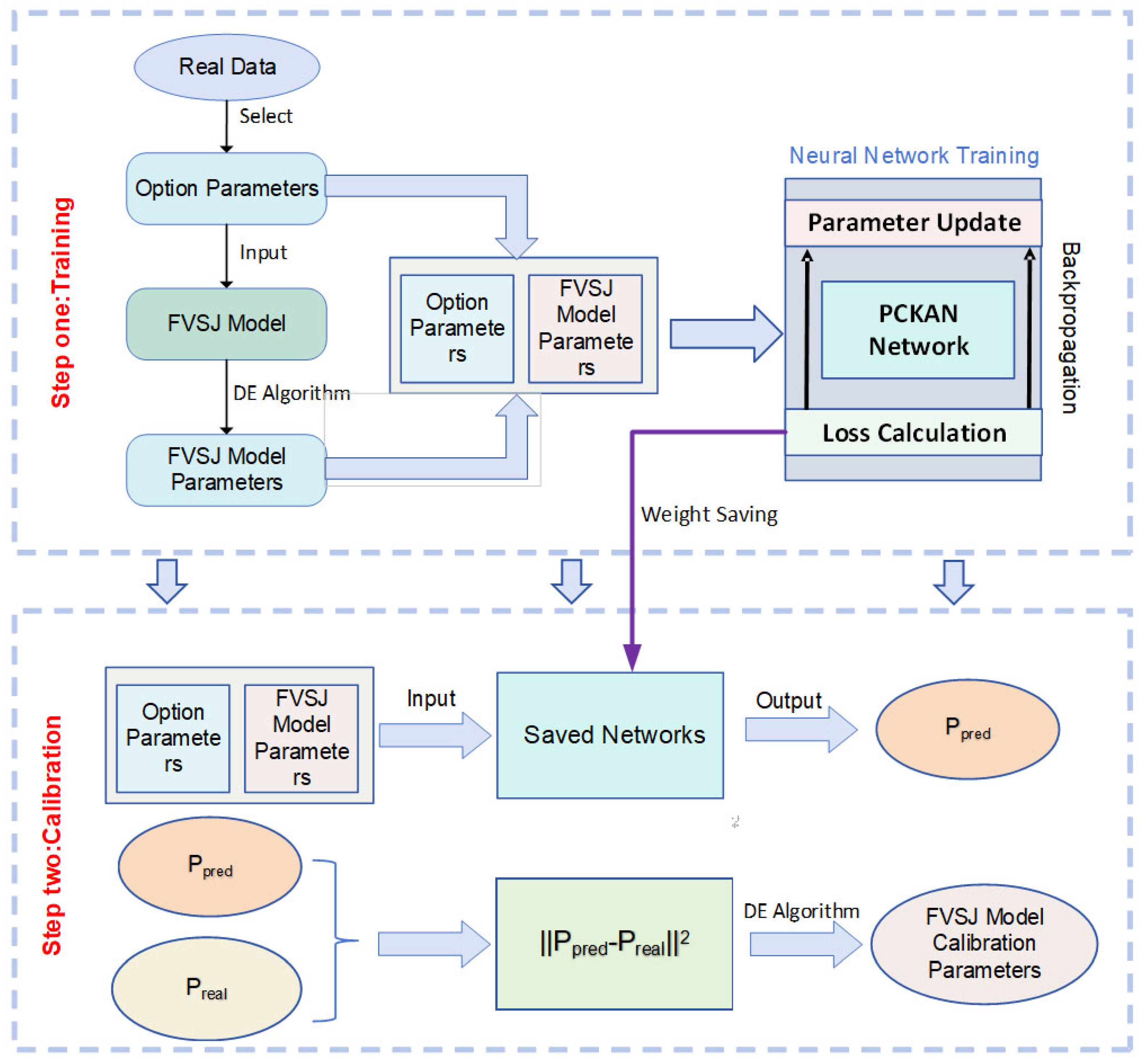
We propose a two-step calibration procedure that integrates PCKAN with the DE algorithm. In step one, PCKAN is trained to approximate the mapping from model parameters and option inputs to option prices. In step two, the trained network serves as a fast surrogate pricer within DE to identify parameter values that best match market quotes. The overall workflow is summarized in Figure 3.
Because real market data do not provide ground-truth parameters, calibration is performed by minimizing pricing errors: an initial parameter estimate is obtained via DE and subsequently refined through further optimization. Algorithm 1 details the proposed two-step procedure for the real-data setting.
Algorithm 1. Two-step calibration via PCKAN and DE.
Input :   Observed   option   quotes   O i r , P i r i = 1 N ;   stochastic   pricing   model   M ( · ) ;   discrepancy   loss   L , ;   physics-informed   loss   L p h y s , ; DE setting.
Output :   Trained   surrogate   f W ;   calibrated   model   parameters   Ω c for new quotes.
Step 1Offline label generation and PCKAN training
Observed   option   quotes   O i r , P i r i = 1 N ;   stochastic   pricing   model   M ( · ) ;   discrepancy   loss   L , ;   physics-informed   loss   L p h y s , .
Extract   option   inputs   O i r   and   corresponding   market   prices   P i r   ( i = 1 , , N )
For   i = 1 , , N   do
Estimate a parameter label by solving
Ω i r = arg   min Ω   L M ( O i r , Ω ) , P i r
where the minimization is performed using DE.
Compute the model-based target price P i m = M ( O i r , Ω )
End For
Form the training set D = ( O i r , Ω i r ) , P i m i = 1 N
Train the PCKAN surrogate f W by minimizing the physics-informed objective
Step 2Online calibration using the trained surrogate
For a new option input data O j r , with its market price P j r calibrate parameters by solving
Ω j c = arg   min Ω   L p h y s f W * O j r , Ω , P j r
where the minimization is performed using DE.
Return Ω j c .

4. Empirical Analysis

4.1. Data and Preprocessing

To evaluate the applicability and robustness of PCKAN in practice, we conduct an empirical study using China 50ETF option data from Yahoo Finance. To ensure data quality and consistency with the model inputs, we apply the following screening rules:
  • Remove option contracts that violate basic no-arbitrage principles, ensuring Equation (21) is satisfied:
    C max ( 0 , S K , S D K e r τ ) ,
    where C denotes the call price and D is the present value of dividends during the option’s life.
  • Remove options with less than 1 day to expiry to avoid interference from accelerated time value decay near expiration and also remove options with more than 255 days to expiry as they are less liquid and have higher premiums.
  • Remove option quotes priced below 0.01, as these quotes are usually within the bid-ask spread and have larger price fluctuations.
  • Remove all option data from half-day trading sessions to ensure complete matching with the underlying asset index’s trading hours.
After screening, the sample contains 38,610 observations, including variables such as option ID, time, contract type, day to expire, spot price, and settle price. For preprocessing, settle Price is standardized using z-score normalization. The data are randomly split into a training set (70%) and a test set (30%). Descriptive statistics are reported in Table 1.

4.2. Evaluation Metrics and Experimental Design

To evaluate PCKAN for model calibration, we implement three surrogate models in PyTorch2.2.2—PCKAN as the proposed method, alongside an MLP and KAN as baseline models—and conduct comparative calibration experiments. For comparability, all three networks adopt almost the same architecture: the input dimension of the Heston model is 10, while that of the FVSJ model is 30 (all including five common features of contractType, dayToExpire, stripPrice, spotPrice, and RFR, with five Heston specific parameters and twenty-five FVSJ parameters added, respectively). The scalar output represents option prices, an input layer, five hidden layers, and an output layer; MLP adopts Softplus activation function. All models were trained using the Adam optimizer, with the Heston model trained for 300 iterations and the FVSJ model trained for 500 iterations, using a gradually decaying learning rate scheduling strategy during the training process. PCKAN is trained using the physical information loss in Equation (20), while MLP, KAN, and CKAN are trained using the mean squared error (MSE) loss shown in Equation (22)
MSE T = 1 n i = 1 n ( y i y ^ i ) 2 ,
where y i and y ^ i denote the true and predicted values for the i -th sample, and n is the number of samples.
The calibration error is measured using three losses, as shown in Equations (23)–(25):
M S E C = 1 N i = 1 N P i T r u e F V S J i ( O , β ) 2
S M A P E = 100 % N i = 1 N P i T r u e F V S J i ( O , β ) P i T r u e + F V S J i ( O , β ) / 2
L o g R M S E = 1 N i = 1 N log P i T r u e log F V S J i ( O , β ) 2
where P i T r u e is the market price, F V S J i ( O , β ) is the output of the network to the FVSJ model, and β denotes the calibrated parameter vector. All experiments are run on a laptop with an Intel Core i7-14650HX CPU (2.20 GHz) and an NVIDIA GeForce RTX 4060 GPU with 8 GB VRAM.

4.3. Experimental Results and Analysis

Table 2 reports the training MSE of MLP, KAN, CKAN, and PCKAN on the empirical Heston and FVSJ datasets.
Table 2 shows that PCKAN achieved the lowest training MSE on both the Heston (1.6 × 10⁻⁴) and FVSJ (3.2 × 10⁻⁴) datasets. CKAN has a slight improvement in accuracy compared to original KAN, but the error is still 2–3 orders of magnitude higher than MLP and PCKAN; PCKAN performs better than the classic MLP benchmark, reducing relative errors by 27.3% and 44.8% on two datasets, respectively, and demonstrating better fitting performance than other models.
Subsequently, calibration experiments were conducted on the trained PCKAN, CKAN, KAN, and MLP neural networks in the Heston dataset and FSVJ dataset validation sets. The calibration error is shown in Table 3.
Table 3 compares the calibration errors of four models on the Heston and FVSJ datasets. The results indicate that the PCKAN proposed in this paper achieved the best performance in terms of MSE, MAPE, and LogRMSE metrics on two datasets. Specifically, compared to the MLP benchmark, the calibration MSE of PCKAN on the Heston and FVSJ datasets decreased by 24.3% and 51.4%, respectively. Compared with CKAN and the original KAN, MSE was reduced by 2–3 orders of magnitude, and the calibration accuracy was better than that of other models.
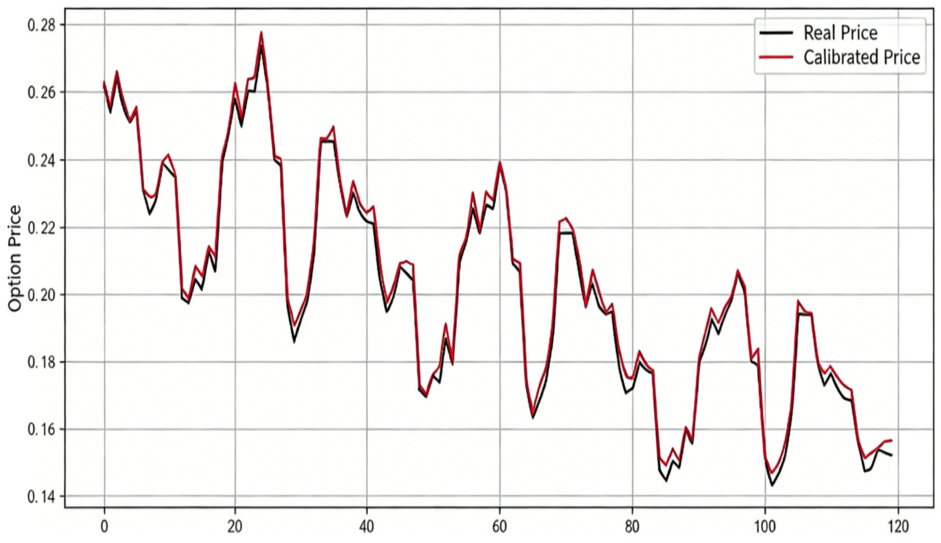
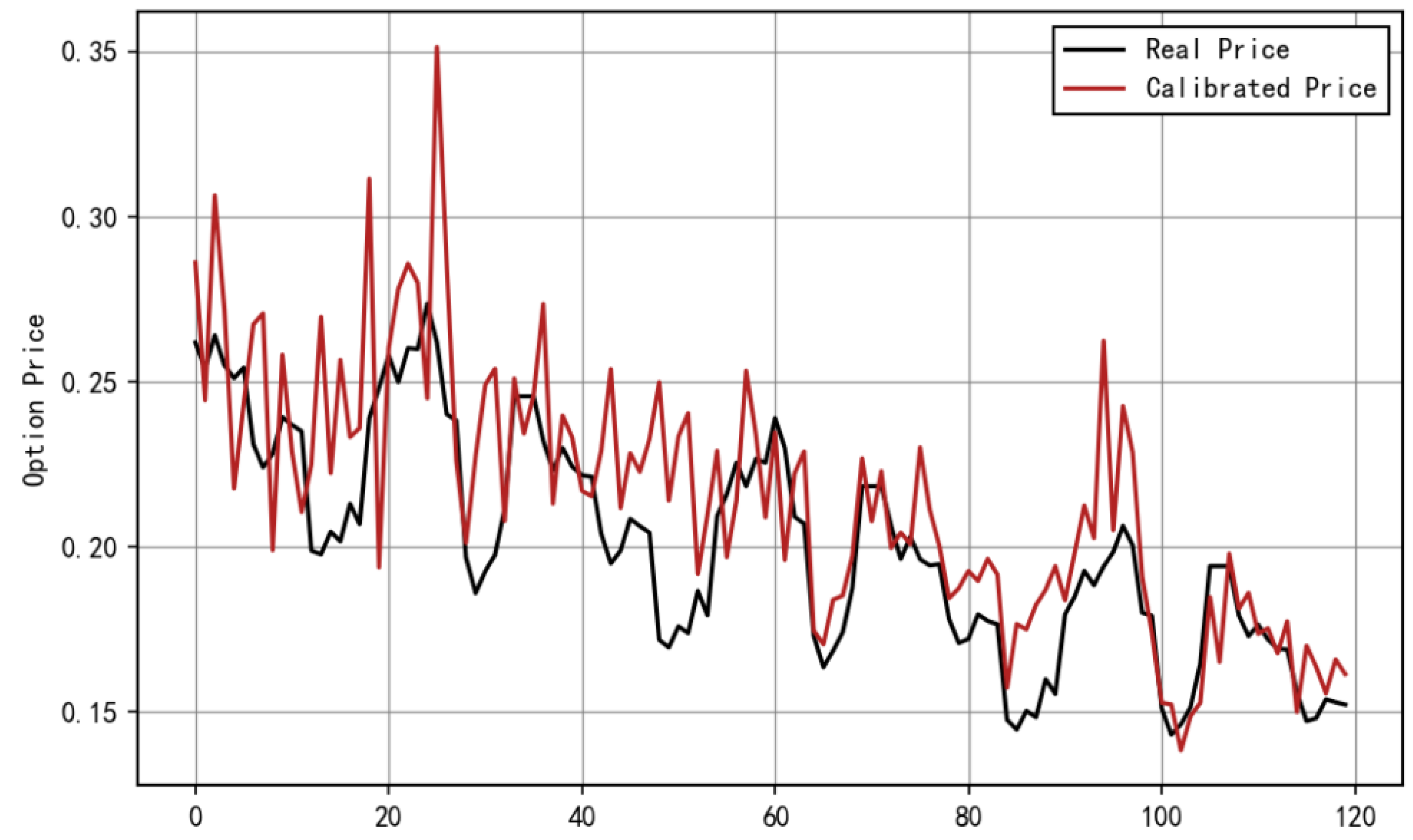
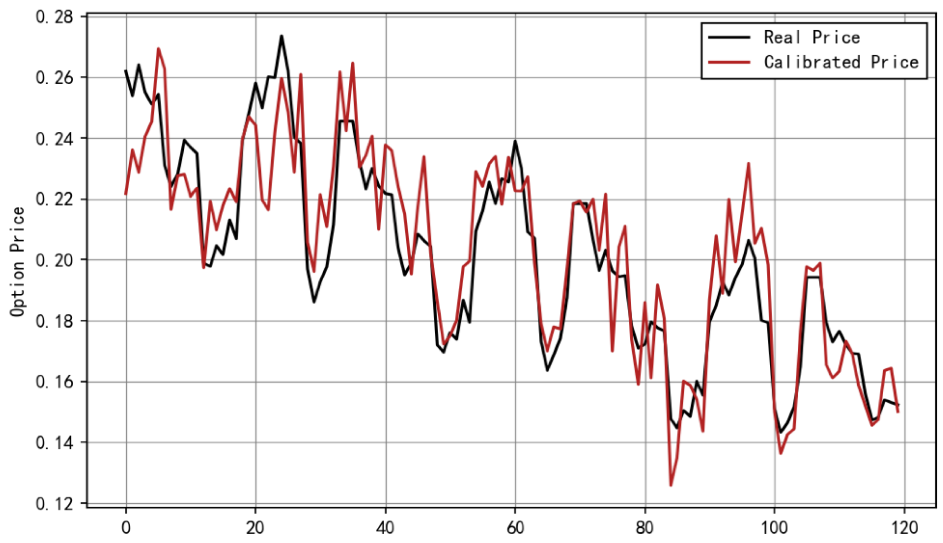
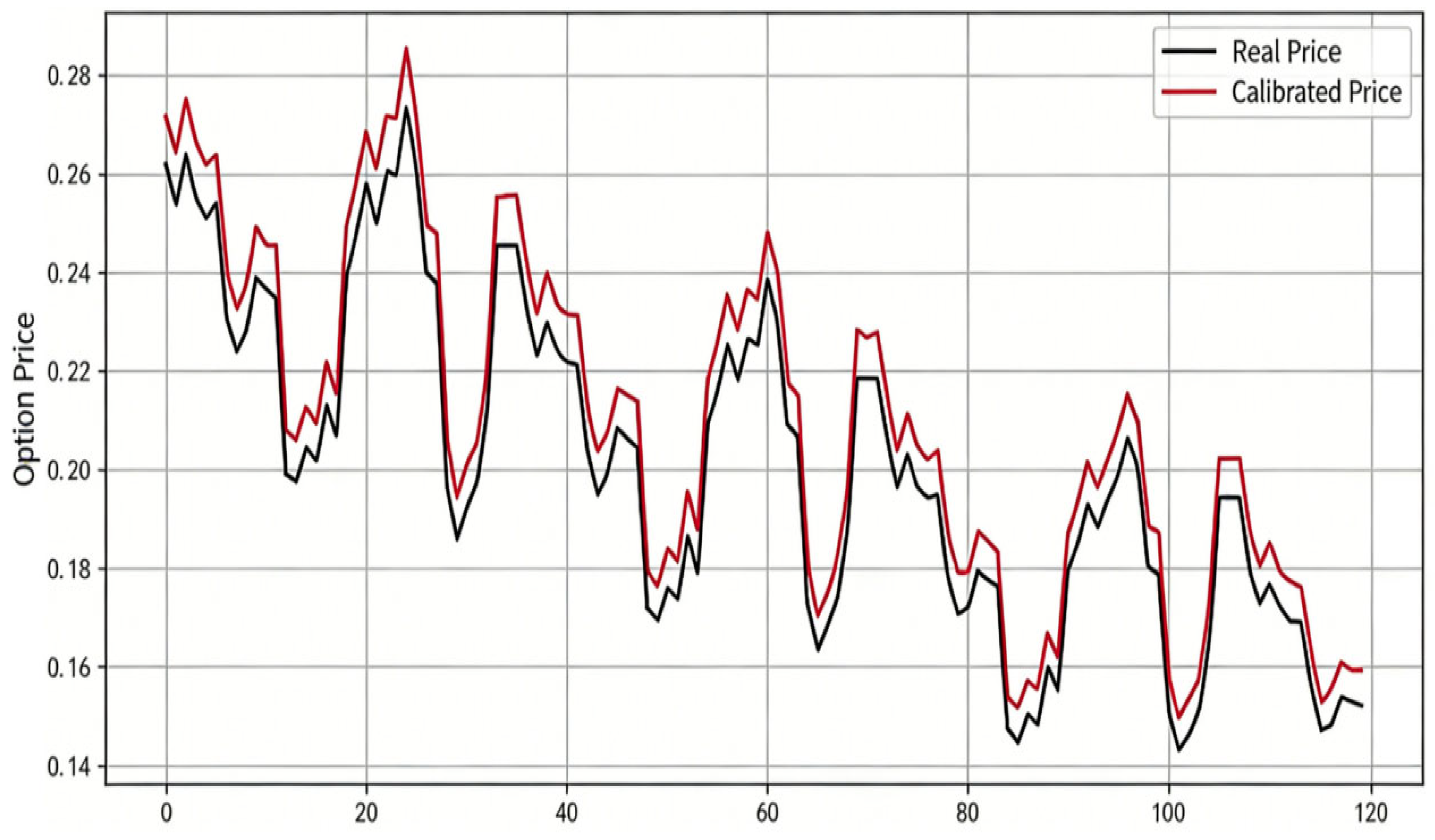
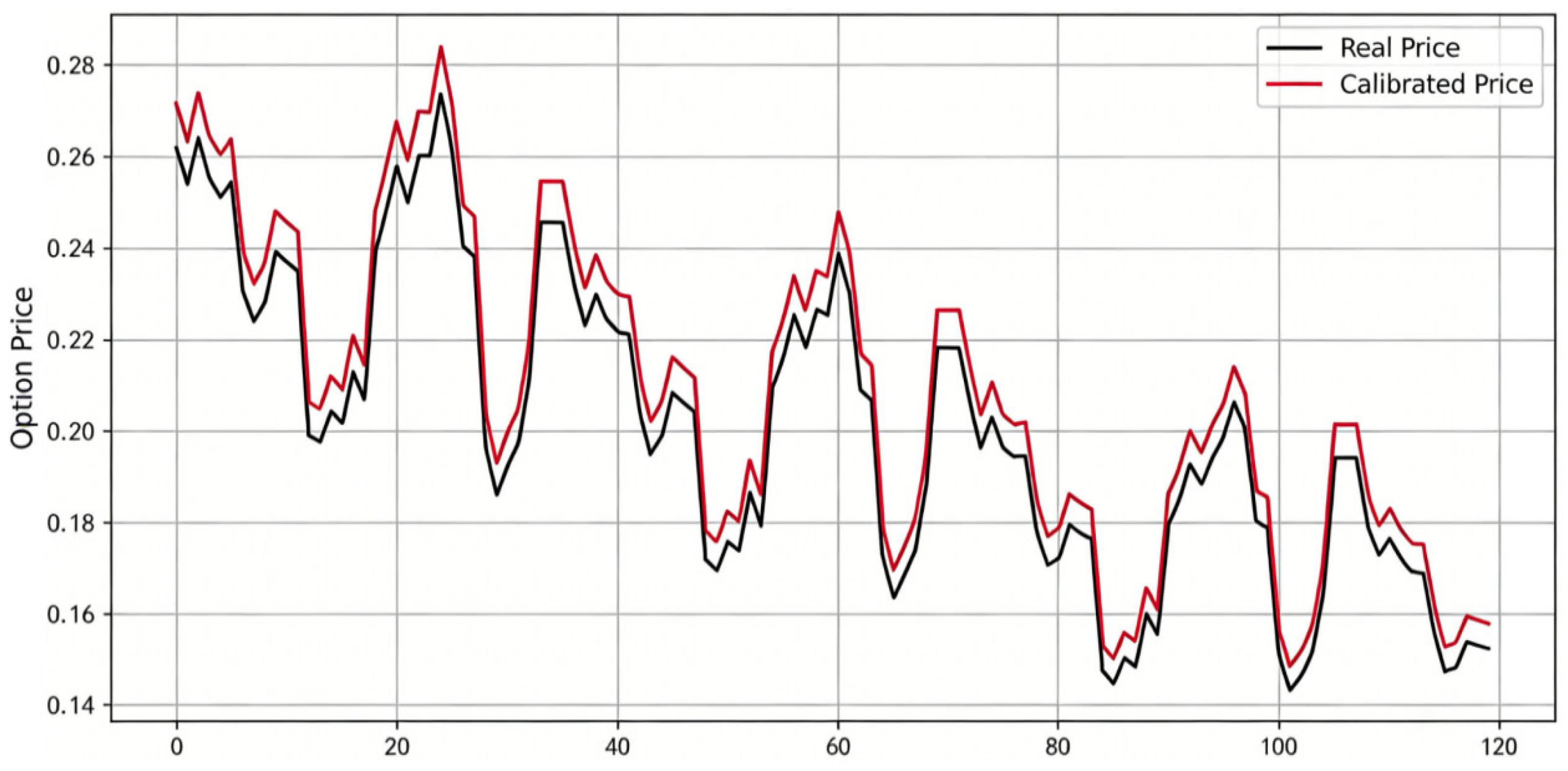
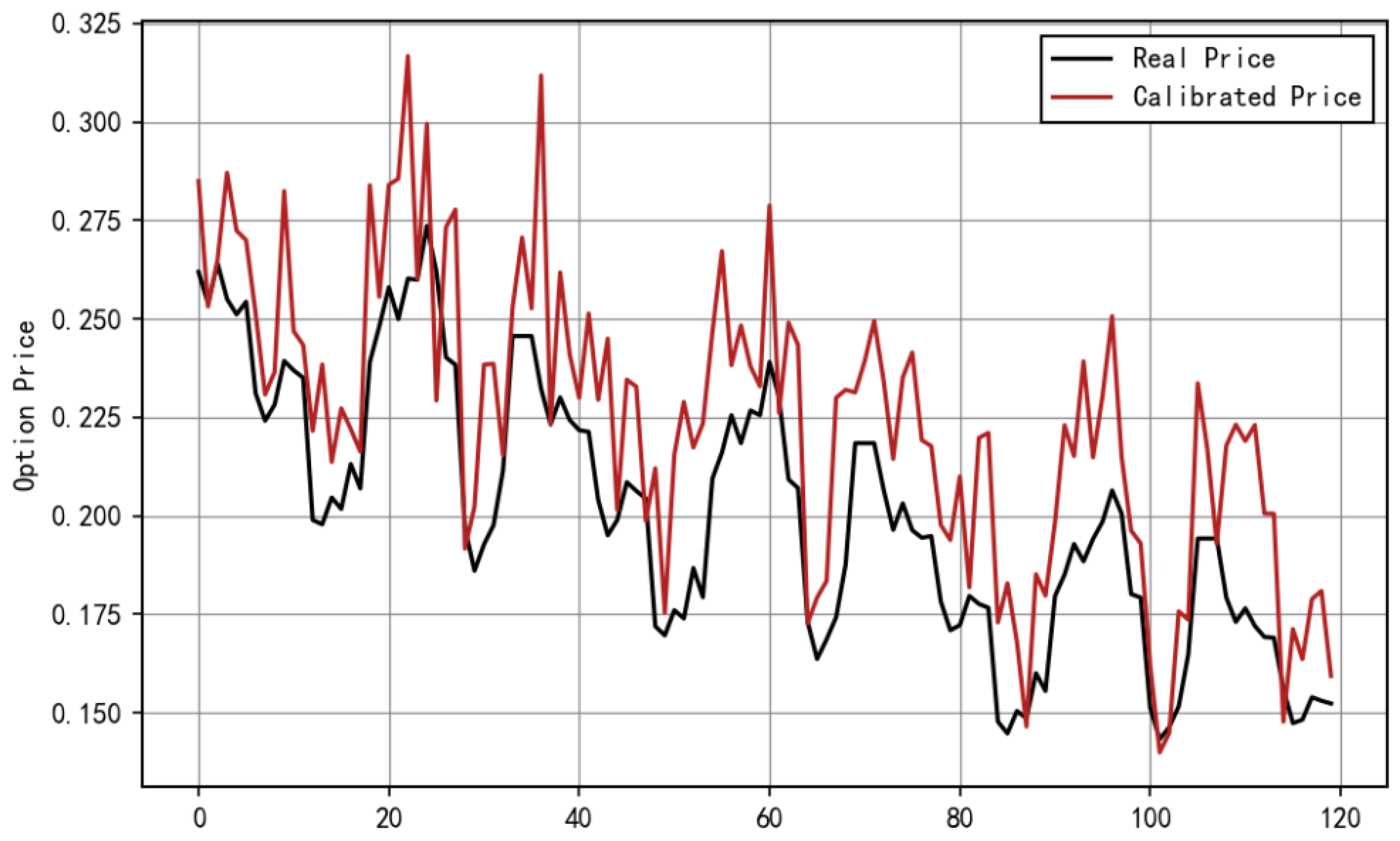
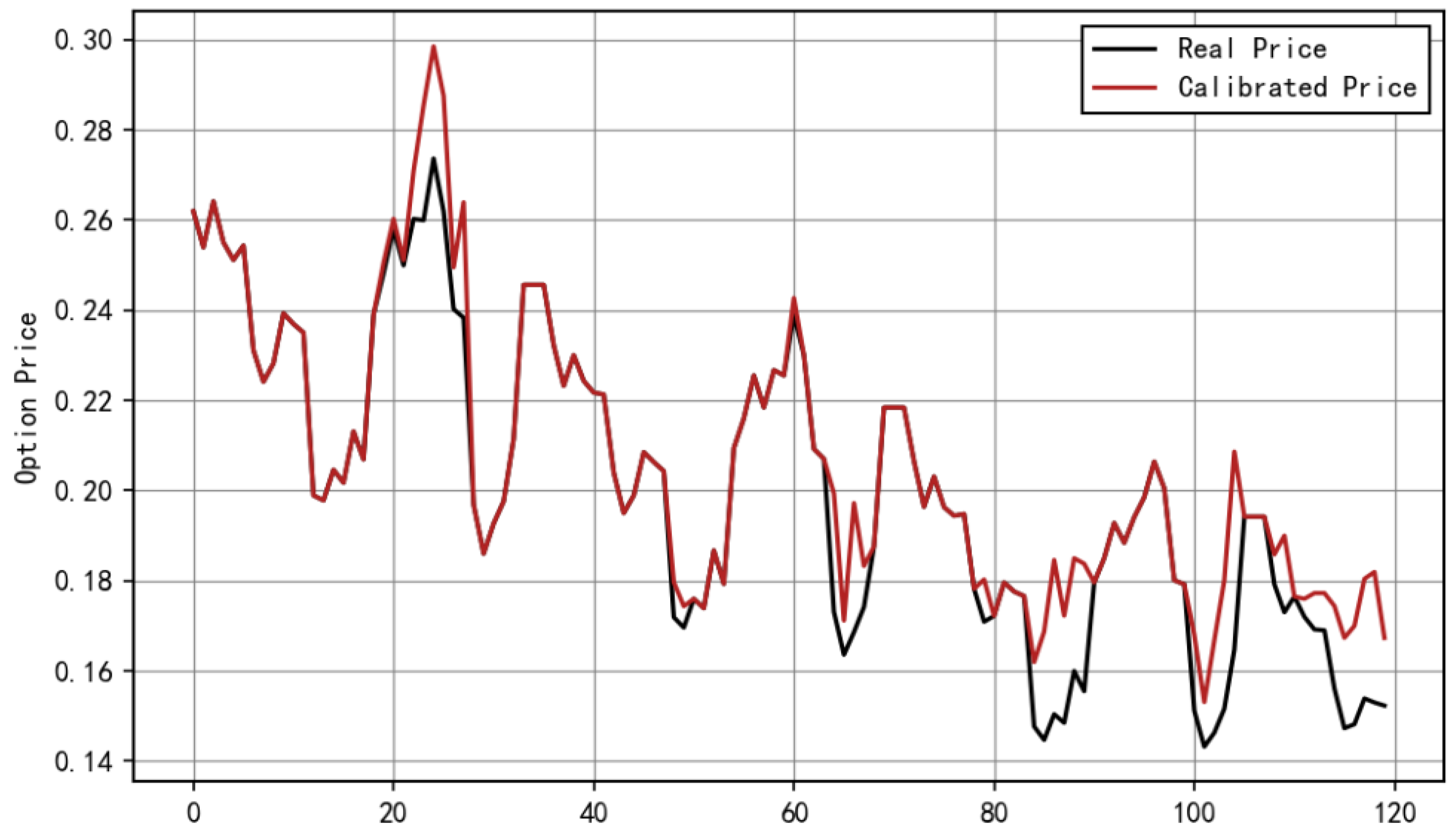
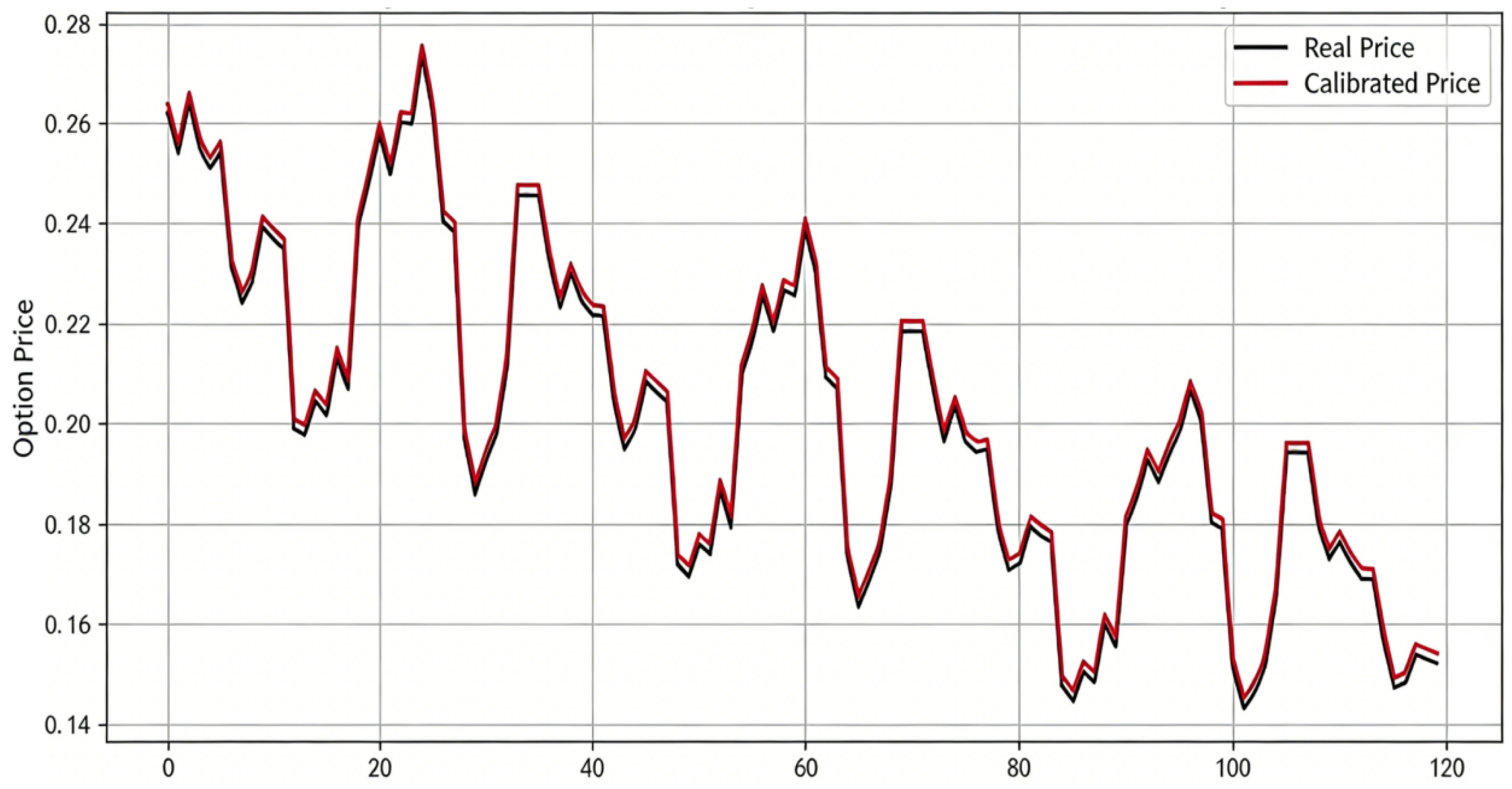
To visually verify the fitting effect and calibration accuracy of the PCKAN framework proposed in this article with benchmark models (MLP, original KAN, CKAN), we compared the fit between the calibrated predicted prices of each model and the real market prices on the FVSJ and Heston datasets, respectively. The results are shown in Figure 4, Figure 5, Figure 6, Figure 7, Figure 8, Figure 9, Figure 10 and Figure 11.
Figure 4, Figure 5, Figure 6 and Figure 7 shows the fitting performance of the original KAN, CKAN, MLP, and PCKAN model on the Heston dataset. The original KAN has the largest deviation from the real price and cannot capture the nonlinear features of the model; CKAN has slight optimization compared to the original KAN, but there are still systematic deviations; MLP performs better than the previous two, but there is still a persistent bias, and the misalignment of high-volatility intervals intensifies. The PCKAN proposed in this article has the highest fitting degree with the actual price, the smallest deviation, and maintains a stable fitting effect within a high fluctuation range, which is consistent with the error index in Table 3.
Figure 8, Figure 9, Figure 10 and Figure 11 show the fitting performance of the original KAN, CKAN, MLP, and PCKAN models on the FVSJ dataset. The native KAN has the largest deviation from the real price and cannot capture the strong nonlinear features of the model; CKAN shows slight improvement compared to native KAN, but lacks adaptability to complex nonlinear scenarios; MLP performs better than the previous two, but compared to the Heston dataset, the fitting bias is significantly amplified, and there is still persistent misalignment; PCKAN maintained the optimal fitting effect, with a high degree of fit between the entire sample interval and the true price, and maintained stable performance in low-bias and high-volatility intervals even in strongly nonlinear scenarios.
The above comparison results are consistent with the error indicators in Table 3, and each model shows different fitting performance on both datasets. PCKAN achieved better fitting results with market option prices in the full sample interval of two datasets, and maintained stable performance in the high-volatility market interval, which is consistent with the expected effect of the model.
Based on a systematic evaluation of the pricing accuracy of each model, we further conducted experiments on pricing efficiency to measure the actual performance of the model in terms of computational cost and operating speed. Due to the poor performance of KAN and CKAN, they were excluded from the subsequent comparison of calibration time. Table 4 shows the calibration time of PCKAN, MLP, and the benchmark method on different datasets, where the benchmark method refers to using differential evolution algorithms to perform nonlinear least squares calibration on the dataset corresponding to each random model.
Table 4 reports the average calibration time each observation. For the Heston dataset, PCKAN requires 7 s each calibration, compared with 3 s for MLP and 34 s for the benchmark method. For the FVSJ dataset, the corresponding times are 37 s, 17 s, and 740 s, respectively. Although PCKAN is slower than MLP, it substantially reduces runtime relative to the benchmark method by factors of 4.9 (Heston) and 20.0 (FVSJ).
To illustrate the scalability implications of this efficiency gain, calibrating the full FVSJ sample on identical computing hardware takes approximately 40 h using the proposed PCKAN framework, compared to roughly 330 h using the benchmark method. This corresponds to an 8.25-fold reduction in total wall-clock time. These results demonstrate that the benchmark method is computationally prohibitive for large-scale batch calibration tasks, while the PCKAN framework delivers a far more practical runtime for high-volume option model calibration.

5. Conclusions

This study proposes a two-step calibration framework based on a Physics-Informed Chebyshev Kolmogorov–Arnold Network (PCKAN) to improve the efficiency–accuracy balance in calibrating the FVSJ model. The framework replaces the B-spline basis in KAN with second-kind Chebyshev polynomials to reduce computational overhead and incorporates Black–Scholes partial differential equation constraints to impose pricing structure. PCKAN is trained offline as a surrogate for the FVSJ pricer and then used online for fast parameter calibration with regard to market quotes.

Empirical experiments are used to evaluate the method. Across the Heston and FVSJ settings, PCKAN yields lower training and calibration errors than the multilayer perceptron and the original KAN under the same experimental configuration, while substantially reducing runtime relative to benchmark calibration based on repeated model pricing. The empirical results further show that the calibrated prices produced using PCKAN track observed market prices across different market regimes.
The PCKAN two-step calibration framework proposed in this study provides empirical support for effective option pricing model calibration, but it still has three limitations. Firstly, the random dataset partitioning does not take into account the time series characteristics of option data when verifying the global fitting ability of the model, which deviates from actual market calibration practices. Secondly, the current validation is limited to standard European options and has not yet been extended to non-standard exotic options, which makes the generality of this method untested in complex derivative scenarios. Thirdly, the physical constraints, based on Black Scholes PDE, only serve as a basic arbitrage-free regularizer and do not include the partial integral differential equations corresponding to the jump and wave diffusion components of the FVSJ model. The above limitations will be addressed in future research.

Author Contributions

Conceptualization, S.Z.; Formal analysis, S.Z. and T.W.; Methodology, Y.G.; Validation, S.Z. and H.X.; Writing—original draft, T.W.; Writing—review & editing, H.X. and W.X. All authors have read and agreed to the published version of the manuscript.

Funding

This work is funded by the National Natural Science Foundation (No. 12401502) and the Natural Science Foundation of Shaanxi Province (No. 2024JC-YBMS-008).

Data Availability Statement

The data presented in this study are openly available in Yahoo Finance at https://finance.yahoo.com/ (accessed on 12 May 2025).

Conflicts of Interest

The authors declare no conflicts of interest.

References

  1. Black, F.; Scholes, M. The pricing of options and corporate liabilities. J. Political Econ. 1973, 81, 637–654. [Google Scholar] [CrossRef] [Scilit] [PubMed]
  2. Hoang, T.M. Long-horizon asset and portfolio returns revisited: Evidence from US markets. Cogent Econ. Financ. 2023, 10, 2238147. [Google Scholar] [CrossRef] [Scilit]
  3. De Domenico, F.; Livan, G.; Montagna, G.; Nicrosini, O. Modeling and simulation of financial returns under non-Gaussian distributions. Phys. A Stat. Mech. Its Appl. 2023, 622, 128886. [Google Scholar] [CrossRef] [Scilit]
  4. Chong, C.H.; Todorov, V. Volatility of volatility and leverage effect from options. J. Econom. 2024, 240, 105669. [Google Scholar] [CrossRef] [Scilit]
  5. Alraddadi, R. The logTG-SV model: A threshold-based volatility framework with logarithmic shocks for exchange rate dynamics. AIMS Math. 2025, 10, 19495–19511. [Google Scholar] [CrossRef] [Scilit]
  6. Kalovwe, S.K.; Mwaniki, J.I.; Simwa, R.O. On regime-switching European option pricing. Cogent Econ. Financ. 2023, 11, 2203439. [Google Scholar] [CrossRef] [Scilit]
  7. Singh, A.; Jha, A.K.; Kumar, A.N. Prediction of cryptocurrency prices through a path dependent Monte Carlo simulation. Commun. Stat.-Simul. Comput. 2025, 1–20. [Google Scholar] [CrossRef] [Scilit]
  8. Yue, C.; Shen, C. Fractal barrier option pricing under sub-mixed fractional Brownian motion with jump processes. AIMS Math. 2024, 9, 31010–31029. [Google Scholar] [CrossRef] [Scilit]
  9. Zhang, S.; Yong, H.; Xiao, H. Option pricing with fractional stochastic volatilities and jumps. Fractal Fract. 2023, 7, 680. [Google Scholar] [CrossRef] [Scilit]
  10. Merton, R.C. Option pricing when underlying stock returns are discontinuous. J. Financ. Econ. 1976, 3, 125–144. [Google Scholar] [CrossRef] [Scilit]
  11. Kou, S.G. A jump diffusion model for option pricing. Manag. Sci. 2002, 48, 1086–1101. [Google Scholar] [CrossRef] [Scilit]
  12. Cai, N.; Kou, S.G. Pricing Asian options under a hyper-exponential jump diffusion model. Oper. Res. 2012, 60, 64–77. [Google Scholar] [CrossRef] [Scilit]
  13. Cai, N.; Kou, S.G. Option pricing under a mixed-exponential jump diffusion model. Manag. Sci. 2011, 57, 2067–2081. [Google Scholar] [CrossRef] [Scilit]
  14. Gatheral, J.; Jaisson, T.; Rosenbaum, M. Volatility is rough. In Commodities; Chapman and Hall/CRC: Boca Raton, FL, USA, 2022; pp. 659–690. [Google Scholar]
  15. Fukasawa, M. Volatility has to be rough. Quant. Financ. 2021, 21, 1–8. [Google Scholar] [CrossRef] [Scilit]
  16. Cox, J.C.; Ross, S.A. The valuation of options for alternative stochastic processes. J. Financ. Econ. 1976, 3, 145–166. [Google Scholar] [CrossRef] [Scilit]
  17. White, A.D.; Hull, J.C. The pricing of options on assets with stochastic volatilities. J. Financ. 1987, 42, 281–300. [Google Scholar]
  18. Heston, S.L. A closed-form solution for options with stochastic volatility with applications to bond and currency options. Rev. Financ. Stud. 1993, 6, 327–343. [Google Scholar] [CrossRef] [Scilit]
  19. Wang, X.; Xiao, W.; Yu, J. Modeling and forecasting realized volatility with the fractional Ornstein Uhlenbeck process. J. Econom. 2023, 232, 389–415. [Google Scholar] [CrossRef] [Scilit]
  20. Zhang, S.; Xiao, H.; Yong, H. Forward Starting Option Pricing under Double Fractional Stochastic Volatilities and Jumps. Fractal Fract. 2024, 8, 283. [Google Scholar] [CrossRef] [Scilit]
  21. Christoffersen, P.; Heston, S.; Jacobs, K. The shape and term structure of the index option smirk: Why multifactor stochastic volatility models work so well. Manag. Sci. 2009, 55, 1914–1932. [Google Scholar] [CrossRef] [Scilit]
  22. Zhang, S.; Sun, Y. Forward starting options pricing with double stochastic volatility, stochastic interest rates and double jumps. J. Comput. Appl. Math. 2017, 325, 34–41. [Google Scholar] [CrossRef] [Scilit]
  23. Lin, A.; Tolooshams, B.; Atchadé, Y.; Ba, D.E. Probabilistic Unrolling: Scalable, Inverse-Free Maximum Likelihood Estimation for Latent Gaussian Models. In Proceedings of the 40th International Conference on Machine Learning, Honolulu, HI, USA, 23–29 July 2023; pp. 21153–21182. [Google Scholar]
  24. Mulenga, N.M.; Fu, Y. Dynamic calibration based on the Black-Scholes option pricing model by Bayesian method. IEEE Access 2024, 12, 119314–119326. [Google Scholar] [CrossRef] [Scilit]
  25. Hilliard, J.E.; Hilliard, J.; Ngo, J.T.D. Implied parameter estimation for jump diffusion option pricing models: Pricing accuracy and the role of loss and evaluation functions. J. Commod. Mark. 2024, 35, 100408. [Google Scholar] [CrossRef] [Scilit]
  26. Bukh, A.V.; Kashtanova, S.V.; Shepelev, I.A. Complex error minimization algorithm with adaptive change rate. Chaos Solitons Fractals 2023, 176, 114154. [Google Scholar] [CrossRef] [Scilit]
  27. Gao, J.; Jia, R.; Noorani, I.; Mehrdoust, F. Calibration of European option pricing model in uncertain environment: Valuation of uncertainty implied volatility. J. Comput. Appl. Math. 2024, 447, 115890. [Google Scholar] [CrossRef] [Scilit]
  28. Joseph, B.; Loeper, G.; Obłój, J. Joint calibration of local volatility models with stochastic interest rates using semimartingale optimal transport. Quant. Financ. 2024, 24, 1597–1620. [Google Scholar] [CrossRef] [Scilit]
  29. Shi, Y.; Teng, B.; Wang, S. Option pricing mechanisms driven by backward stochastic differential equations. Financ. Innov. 2025, 11, 90. [Google Scholar] [CrossRef] [Scilit]
  30. Büchel, P.; Kratochwil, M.; Nagl, M.; Rösch, D. Deep calibration of financial models: Turning theory into practice. Rev. Deriv. Res. 2022, 25, 109–136. [Google Scholar] [CrossRef] [Scilit] [PubMed]
  31. Dadah, S. Deep Calibration of Option Pricing Models. Master’s Thesis, University of Cape Town, Cape Town, South Africa, 2022. [Google Scholar]
  32. Horvath, B.; Muguruza, A.; Tomas, M. Deep learning volatility: A deep neural network perspective on pricing and calibration in (rough) volatility models. Quant. Financ. 2021, 21, 11–27. [Google Scholar] [CrossRef] [Scilit]
  33. Gazzani, G.; Guyon, J. Pricing and calibration in the 4-factor path-dependent volatility model. Quant. Financ. 2025, 25, 471–489. [Google Scholar] [CrossRef] [Scilit]
  34. Liu, Z.; Wang, Y.; Vaidya, S.; Ruehle, F.; Halverson, J.; Soljačić, M.; Hou, T.Y.; Tegmark, M. Kan: Kolmogorov-arnold networks. arXiv 2024, arXiv:2404.19756. [Google Scholar]
  35. Thao, T.H. An approximate approach to fractional analysis for finance. Nonlinear Anal. Real World Appl. 2006, 7, 124–132. [Google Scholar] [CrossRef] [Scilit]
  36. Fang, F.; Oosterlee, C.W. A novel pricing method for European options based on Fourier-cosine series expansions. SIAM J. Sci. Comput. 2008, 31, 826–848. [Google Scholar] [CrossRef] [Scilit]
  37. Kim, S.; Yun, S.B.; Bae, H.O.; Lee, M.; Hong, Y. Physics-informed convolutional transformer for predicting volatility surface. Quant. Financ. 2024, 24, 203–220. [Google Scholar] [CrossRef] [Scilit]
Figure 1. Schematic diagram of overall structure of KAN neural network produced on Chebyshev basis.
Mathematics 14 01529 g001
Figure 2. PCKAN data flow diagram.
Mathematics 14 01529 g002
Figure 3. Two-step calibration flowchart.
Mathematics 14 01529 g003
Figure 4. KAN: Predicted vs. market option prices on the Heston dataset.
Mathematics 14 01529 g004
Figure 5. CKAN: Predicted vs. market option prices on the Heston dataset.
Mathematics 14 01529 g005
Figure 6. MLP: Predicted vs. market option prices on the Heston dataset.
Mathematics 14 01529 g006
Figure 7. PCKAN: Predicted vs. market option prices on the Heston dataset.
Mathematics 14 01529 g007
Figure 8. KAN: Predicted vs. market option prices on the FVSJ dataset.
Mathematics 14 01529 g008
Figure 9. CKAN: Predicted vs. market option prices on the FVSJ dataset.
Mathematics 14 01529 g009
Figure 10. MLP: Predicted vs. market option prices on the FVSJ dataset.
Mathematics 14 01529 g010
Figure 11. PCKAN: Predicted vs. market option prices on the FVSJ dataset.
Mathematics 14 01529 g011
Table 1. Descriptive statistics of the empirical dataset.
DatasetBasic DataMeanVarianceMaximumMinimum
Day to Expire87.1365.70244.01.0
TrainingSpot Price2.570.163.02.3
Settle Price0.180.190.980.01
Day to Expire95.9865.14244.01.0
TestSpot Price2.870.133.12.6
Settle Price0.170.160.970.01
Table 2. Training MSE of MLP, KAN, CKAN, and PCKAN on the Heston and FVSJ datasets.
DatasetMLPKANCKANPCKAN
Heston2.2 × 10−47.4 × 10−26.8 × 10−31.6 × 10⁻⁴
FVSJ5.8 × 10−49.0 × 10−28.4 × 10−33.2 × 10⁻⁴
Table 3. Comparison of calibration errors for MLP, KAN, CKAN, and PCKAN on the Heston and FVSJ datasets.
DatasetNeural NetworkMSECSMAPELogRMSE
HestonPCKAN5.66040 × 10−50.036250.03625
CKAN2.20530 × 10−30.058460.07104
KAN8.80880 × 10−30.099550.12889
MLP7.47842 × 10−50.041790.04190
FVSJPCKAN4.00039 × 10−60.010170.01031
CKAN1.29590 × 10−30.030630.06345
KAN8.57170 × 10−30.115550.13682
MLP8.22945 × 10−60.015030.01245
Table 4. The time spent on each calibration of PCKAN, MLP, and benchmark methods.
DatasetMLPPCKANBenchmark Method
Heston7334
FVSJ3717740
Disclaimer/Publisher’s Note: The statements, opinions and data contained in all publications are solely those of the individual author(s) and contributor(s) and not of MDPI and/or the editor(s). MDPI and/or the editor(s) disclaim responsibility for any injury to people or property resulting from any ideas, methods, instructions or products referred to in the content.