Machine Learning Hazard Estimation with Valid Bootstrap Inference for Generalized Progressive Hybrid Censoring

Abstract

Reliability studies frequently employ progressive censoring schemes that remove surviving units during testing, yet statistical inference under such designs remains vulnerable to parametric model misspecification. When distributional assumptions fail, conventional maximum likelihood estimators converge to systematically biased limits, producing confidence intervals with severely degraded coverage. We develop a flexible inferential framework that models the hazard function through a neural network architecture, avoiding commitment to a parametric family. To quantify uncertainty, we introduce a stratified weighted bootstrap procedure that preserves the dependency structure induced by progressive removals. We establish that the proposed estimator achieves the minimax optimal nonparametric rate $n^{-\alpha /(2\alpha +1)}$ for $\alpha$-smooth hazard functions and prove that the bootstrap consistently approximates the sampling distribution, yielding asymptotically valid pointwise confidence intervals for the survival function. A local asymptotic analysis precisely characterizes the efficiency–robustness tradeoff. Comprehensive simulations comparing against parametric methods, penalized splines, piecewise exponential models, and kernel estimators demonstrate that our method maintains 92–94% coverage under misspecification, whereas parametric alternatives collapse to 40–45% and simpler nonparametric methods achieve only 85–91%. The neural network architecture provides 23–29% lower integrated mean squared error than penalized splines using the same bootstrap, confirming that both components of our framework contribute to performance. Computational requirements remain practical: parallelized bootstrap inference completes in under 25 s on an 8-core processor for typical sample sizes. Application to electronic component lifetime data illustrates how the methodology yields materially different reliability assessments with direct implications for warranty planning.

1. Introduction

The analysis of time-to-event data occupies a central place in statistical methodology, with applications spanning engineering reliability, clinical medicine, actuarial science, and beyond. A defining feature of such data is censoring: the event of interest remains unobserved for some subjects due to study termination, loss to follow-up, or deliberate experimental design. While classical right-censoring has received extensive theoretical treatment, modern testing environments increasingly employ more sophisticated censoring mechanisms that balance inferential goals against practical resource constraints. Progressive censoring schemes, which permit the removal of surviving units at intermediate failure times, exemplify this development. These designs offer practitioners flexibility in managing test duration and equipment utilization while still extracting meaningful reliability information from the observed failures.

The appeal of progressive censoring has motivated a substantial literature on parametric inference under such designs. Given observed failure times and removal patterns, analysts typically specify a distributional family for the underlying lifetimes and proceed with likelihood-based estimation. This approach enjoys well-understood optimality properties when the assumed model coincides with the true data-generating process. The maximum likelihood estimator achieves the Cramér-Rao lower bound, confidence intervals attain nominal coverage, and hypothesis tests control Type I error at the specified level. These guarantees, however, rest upon correct model specification, an assumption that proves difficult to verify in practice and potentially consequential when violated.

The consequences of model misspecification in censored data settings deserve careful attention. Unlike estimation problems with complete data, where nonparametric alternatives provide natural robustness, the complex dependency structure induced by progressive censoring complicates the development of flexible methods. When the parametric assumption fails, the maximum likelihood estimator no longer targets the true parameter but instead converges to a pseudo-true value that minimizes Kullback–Leibler divergence to the assumed family. This systematic bias persists regardless of sample size, meaning that increased data collection cannot correct the fundamental error. More troubling still, standard confidence intervals, constructed under the false assumption of correct specification, exhibit coverage probabilities that may fall dramatically below nominal levels. For reliability applications where inference guides warranty policies, maintenance schedules, and safety assessments, such inferential failures carry tangible consequences.

Existing approaches to robust survival inference face limitations when applied to progressive censoring contexts. The celebrated Kaplan–Meier estimator and its associated variance calculations assume independent censoring that does not depend on the failure time distribution, a condition violated by progressive designs where removals occur at observed failure times. Semiparametric methods based on Cox regression accommodate flexible baseline hazards but require covariate information and proportional hazards structure that may be absent or inappropriate in reliability settings. Bayesian nonparametric approaches offer another avenue toward flexibility, yet their theoretical properties under progressive censoring remain incompletely understood, and computational demands may preclude routine application. The analyst confronting progressively censored data thus faces an uncomfortable choice: adopt parametric methods with their attendant misspecification risks, or apply methods designed for simpler censoring mechanisms and hope the approximation suffices.

This paper develops an alternative framework that combines flexible hazard estimation with principled uncertainty quantification tailored to progressive censoring schemes. Our approach models the hazard function through a feedforward neural network, a choice motivated by the universal approximation capabilities of such architectures. By parameterizing the hazard directly rather than assuming membership in a finite-dimensional family, the estimator can adapt to monotonic, bathtub-shaped, or multimodal hazard patterns without prior specification. The network parameters are estimated by minimizing a loss function derived from the progressive censoring likelihood, ensuring that the estimation procedure respects the observed data structure. To construct confidence intervals and perform inference, we introduce a stratified weighted bootstrap that accounts for the risk-set dynamics inherent to progressive designs. The stratification preserves the information content of different removal patterns, while the weighting scheme reflects the number of units represented by each observed failure.

The theoretical development establishes that this framework delivers on its inferential promises. We prove that the neural hazard estimator converges to the true hazard function at the minimax optimal rate $n^{-\alpha /(2\alpha +1)}$ for hazard functions with smoothness index $\alpha$, which is slower than the parametric $\sqrt{n}$-rate but does not require correct model specification. The stratified bootstrap is shown to consistently approximate the sampling distribution of the survival function estimator, validating its use for pointwise confidence interval construction. Perhaps most importantly, we characterize the efficiency–robustness tradeoff through a local asymptotic analysis. When the parametric model happens to be correct, our flexible estimator incurs a modest efficiency loss relative to the oracle maximum likelihood estimator. Under local misspecification, however, the parametric approach accumulates bias that eventually dominates its variance advantage, while our method remains approximately unbiased. This analysis provides practitioners with a principled basis for preferring robust methods when model uncertainty is present.

Numerical studies corroborate the theoretical findings and demonstrate practical relevance. We conduct comprehensive simulations comparing our method against not only parametric approaches but also flexible nonparametric alternatives—penalized splines with the same bootstrap procedure, piecewise exponential models, and kernel hazard estimators. This comparison addresses a natural question: does the neural network architecture provide meaningful improvements, or would simpler flexible methods suffice? Our results demonstrate that both components of the framework contribute to performance. The neural network achieves 23–29% lower integrated mean squared error than penalized splines under misspecification, while maintaining superior coverage probability (92–94% versus 85–91%). We further investigate robustness to violations of our smoothness assumptions, showing graceful degradation under discontinuous hazard functions. Application to electronic component lifetime data illustrates how the methodological differences translate into distinct reliability assessments with direct financial implications for warranty planning. Computational requirements, while higher than parametric methods, remain practical: parallelized bootstrap inference completes in under 25 s for typical sample sizes.

The remainder of this paper proceeds as follows. Section 2 reviews related work on progressive censoring, nonparametric survival estimation, and neural network approaches to hazard modeling. Section 3 formalizes the censoring mechanism, develops the neural hazard network estimator, and introduces the stratified weighted bootstrap procedure. Section 4 establishes the theoretical properties of our framework, including consistency, bootstrap validity, and the efficiency–robustness tradeoff. Section 5 presents a comprehensive numerical analysis of the results obtained in previous sections. Section 6 applies the methodology to reliability data. Section 7 concludes with discussion and directions for future research.

2. Literature Review

Research on censored data inference has advanced along three broad and interrelated trajectories: (i) parametric inference under progressive censoring designs, (ii) nonparametric and semiparametric survival estimation, and (iii) machine-learning-based hazard modeling paired with resampling-based uncertainty quantification. We organize the review along these lines to clarify the gap our framework addresses before situating our contribution at their intersection.

(i) Progressive censoring: designs and parametric inference: The statistical treatment of progressive censoring originated with [1], who recognized that industrial life testing often involves planned removal of functioning units before study completion. Unlike conventional Type I or Type II censoring, which terminate observation at a fixed time or after a predetermined number of failures, progressive schemes distribute removals across the duration of the experiment. This flexibility permits more efficient resource allocation, as units withdrawn early can be redirected to other testing purposes, while still yielding informative data about the failure time distribution.

Subsequent developments expanded the class of progressive designs to accommodate practical constraints. Ref. [2] investigated progressive Type II hybrid censoring, establishing inferential procedures for exponential lifetimes. Ref. [3] provided a comprehensive treatment of progressive censoring methodology, cataloging results for numerous distributional families and censoring configurations. The hybrid progressive censoring scheme, introduced by [4], combined features of Type I and Type II designs by imposing both a target failure count and a maximum observation time. This innovation addressed situations where testing cannot continue indefinitely regardless of the number of observed failures. For more reading, see Ref. [5].

The generalized progressive hybrid censoring scheme (GPHCS), which forms the setting for our methodology, represents a further refinement proposed by [6]. This design incorporates an additional threshold parameter that governs behavior when few failures occur before the time limit. Specifically, if failures accumulate slowly, the experiment continues beyond the nominal time limit until a minimum number of events have been observed, preventing scenarios where early termination yields insufficient information for meaningful inference. Refs. [6,7] developed exact likelihood inference for exponential lifetimes under GPHCS, while [8] extended these results to the Burr Type-XII distribution. Despite this progress, inference under GPHCS has remained predominantly parametric, leaving open the question of how to proceed when distributional assumptions cannot be confidently maintained.

Parametric methods under progressive censoring achieve excellent efficiency when the assumed distributional family is correct. Ref. [9] established foundational results for exponential and Weibull models; ref. [10] treated two-parameter bathtub-shaped lifetimes; and [11] introduced Gibbs-sampling procedures for Weibull data. However, as [12] demonstrated, when the assumed family is incorrect the MLE converges not to the true parameter but to a pseudo-true value minimizing the Kullback–Leibler (KL) divergence to that family—inducing persistent asymptotic bias that additional data cannot remove. Refs. [13,14] document cases where such misspecification yields materially incorrect reliability predictions with direct consequences for warranty reserves and maintenance planning, motivating the flexible, distribution-free alternatives developed here.

(ii) Nonparametric and semiparametric survival estimation: Classical nonparametric survival analysis, anchored by the Kaplan–Meier estimator [15] and the Nelson–Aalen cumulative hazard estimator [16,17], provides distribution-free inference under independent censoring. The elegant theory supporting these estimators relies critically on the assumption that censoring times are independent of failure times—a foundational requirement formalized in the counting process framework of [17,18]. This condition is satisfied by Type I censoring but violated by progressive designs where removals occur at observed failure times, creating dependence between the censoring mechanism and the failure process. This violation underscores the need for methods tailored to the censoring mechanism at hand.

Semiparametric methods, particularly the Cox proportional hazards model [19], offer flexibility in the baseline hazard while imposing structure through the proportional hazards assumption. Extensions to progressive censoring have been considered by [20], who developed maximum likelihood and Bayesian estimation for the half-logistic distribution under progressive Type II censoring. However, the proportional hazards framework requires covariate information and a multiplicative hazard structure that may be inappropriate for reliability settings where the primary goal is marginal survival estimation rather than covariate effect quantification. Moreover, the baseline hazard, while treated nonparametrically, is typically estimated through a step function that may inadequately capture smooth underlying hazard shapes.

Alternative approaches have been proposed for specific progressive censoring configurations. Ref. [21] developed goodness-of-fit tests for the exponential distribution based on spacings for progressively Type-II censored data. These contributions notwithstanding, a general nonparametric framework for inference under generalized progressive hybrid censoring has remained elusive.

(iii) Neural network hazard estimation: The application of neural networks to survival data has expanded considerably in recent years, driven by the capacity of these models to capture complex nonlinear relationships without explicit parametric specification. Ref. [22] introduced an early neural network extension of the Cox model, replacing the linear predictor with a feedforward architecture while retaining the partial likelihood framework. This work demonstrated that neural networks could improve predictive accuracy when covariate effects departed from linearity, establishing a foundation for subsequent methodological development.

More recent contributions have embraced deeper architectures and more flexible formulations. Ref. [23] proposed DeepSurv, which employs modern optimization techniques and regularization strategies to train Cox-type neural networks on high-dimensional data. Ref. [24] introduced DeepHit, which directly models the probability mass function of discretized survival times, avoiding the proportional hazards assumption entirely. Ref. [25] developed continuous-time neural network models that parameterize the hazard function through a network architecture, an approach conceptually similar to ours though developed for different data structures and without the progressive censoring considerations central to our work. This direction has been further enriched by semi-structured approaches that combine the flexibility of neural networks with the interpretability of classical statistical models [26,27], as well as by applied work demonstrating the practical advantages of machine learning over traditional regression in high-stakes clinical prediction [28].

The theoretical properties of neural network survival estimators have received increasing attention. Ref. [29] established consistency and convergence rates for deep learning estimators in the partially linear Cox model, proving that neural network estimators achieve minimax optimal rates under smoothness assumptions. This work draws on approximation theory for neural networks [30]. Ref. [31] provided a comprehensive systematic review of deep learning methods for survival analysis, characterizing approaches according to both survival-related and deep learning attributes. General frameworks for integrating machine learning with survival analysis have also been proposed [32]. These theoretical and methodological advances provide important precedents for our analysis, though the extension to progressive censoring requires careful attention to the modified likelihood structure and the dependencies introduced by the removal pattern.

The integration of machine learning with classical statistical inference represents a broader methodological trend with applications beyond survival analysis. Ref. [33] recently demonstrated the complementary strengths of Bayesian and machine learning approaches for parameter estimation in queueing systems, showing that neural networks and random forests can outperform traditional maximum likelihood estimation under complex system dynamics and noisy conditions. Their comparative framework, which systematically evaluates classical, Bayesian, and machine learning estimators within a unified experimental design, provides a methodological template that resonates with our approach to survival inference. The finding that machine learning methods exhibit particular advantages when the underlying data-generating process deviates from standard parametric assumptions parallels our motivation for developing flexible hazard estimators robust to model misspecification.

(iv) Bootstrap inference for censored data: Resampling methods have a long history in survival analysis, providing distribution-free approaches to variance estimation and confidence interval construction. Ref. [34] pioneered the application of bootstrap techniques to right-censored data, proposing a resampling scheme that draws failure and censoring times jointly while preserving the censoring indicator. Ref. [35] established theoretical foundations for bootstrap consistency under random censoring, showing that the bootstrap distribution of the Kaplan–Meier estimator converges to the appropriate limit.

Extensions to more complex censoring mechanisms have required modifications to standard resampling schemes. Ref. [36] provided a comprehensive treatment of bootstrap methods for survival data, including adaptations for interval censoring and truncation. Ref. [37] developed resampling-based inference for regression models with censored outcomes, demonstrating that the limiting covariance matrices can be estimated by a resampling technique without nonparametric density estimation. This resampling paradigm has proven particularly valuable when the data structure precludes straightforward case resampling.

For progressive censoring specifically, bootstrap methods remain comparatively underdeveloped. Ref. [3] noted the challenges posed by the dependent removal structure and suggested that naive resampling could distort inferential properties. The stratified weighted bootstrap we propose addresses this gap by incorporating the progressive removal structure directly into the resampling mechanism, preserving the risk-set dynamics that conventional approaches disrupt.

The foregoing review reveals a methodological landscape where substantial progress has been made along separate dimensions, yet integration remains incomplete. Parametric inference under progressive censoring is well developed but vulnerable to misspecification. Nonparametric survival methods offer robustness but have not been adequately adapted to progressive designs. Neural network approaches provide flexible hazard estimation but have not been systematically extended to progressive censoring contexts. Bootstrap methods for censored data exist but lack versions specifically designed for progressive removal structures.

Our contribution occupies the intersection of these research streams. By combining neural network hazard estimation with a stratified weighted bootstrap tailored to progressive censoring, we construct a framework that inherits flexibility from the machine learning literature, inferential validity from bootstrap theory, and practical applicability from the reliability engineering tradition. The theoretical analysis we provide establishes that this synthesis achieves more than a heuristic combination of techniques: the resulting estimator possesses provable consistency and convergence properties, while the bootstrap delivers asymptotically valid confidence intervals. In this sense, our work represents not merely an application of neural networks to a new data structure but a methodological advance that expands the scope of rigorous nonparametric inference for censored data.

3. Preliminaries and Methodology

The statistical challenge posed by generalized progressive hybrid censoring schemes (GPHCSs) requires a precise formulation of the data-generating process, the limitations of standard inference, and the design of a more adaptable alternative. This section provides that foundation. We first formalize the GPHCS experiment and its likelihood, then clarify why traditional parametric inference becomes unreliable under model uncertainty. Finally, we introduce our proposed neural hazard network estimator and the stratified weighted bootstrap procedure, explaining how their construction directly addresses the identified shortcomings.

3.1. Mathematical Framework and Methodology

To develop a robust inference procedure for generalized progressive hybrid censoring schemes (GPHCSs), we must first establish a precise mathematical foundation. This section proceeds in three logical stages. First, we formalize the GPHCS experimental design and its associated likelihood, which is the cornerstone of all subsequent inference. Second, we examine why traditional parametric maximum likelihood estimation, while efficient under correct specification, fails catastrophically under model misspecification—a failure characterized by asymptotic bias. Third, we introduce our proposed solution: a neural network parameterization of the hazard function, paired with a specially designed bootstrap procedure for valid inference. Together, these components form a coherent, assumption-flexible framework for reliability analysis.

3.1.1. Formal Specification of the Censoring Mechanism and Likelihood

The generalized progressive hybrid censoring scheme is designed to balance information acquisition with practical constraints. We begin by defining its components precisely.

Definition 1.

Let $X_1,\dots ,X_n$ represent the independent lifetimes of n testing units, drawn from a continuous distribution F with density f. The experiment is governed by three design parameters: a target number of failures m (where $m\le n$), a threshold k (with $k<m$), and a terminal time $T>0$. Additionally, a progressive censoring scheme $\mathbf{R}=(R_1,\dots ,R_m)$ is predetermined, where each $R_i$ is a non-negative integer and ${\sum }_{i=1}^m{R}_i=n-m$. The experiment terminates at time

$$T^{*}=max\{X_{k:m:n},min\{X_{m:m:n},T\}\},$$

where $X_{i:m:n}$ denotes the i-th ordered failure time. The observed number of failures $D^{*}$ depends on which termination condition triggers first, as detailed in [6].

The observed data therefore consists of $D^{*}$ distinct failure times, each associated with an effective removal count $R_i^{*}$ (adjusted for the realized termination rule), and a set of $R_{\tau }^{*}$ units censored at the terminal time $T^{*}$. For inference within a parametric family $\{F_{\theta }:\theta \in \mathrm{\Theta }\subset {\mathbb{R}}^p\}$, the likelihood function consolidates this complex censoring information into a single expression.

Definition 2.

For a parametric model with density $f_{\theta }$ and distribution $F_{\theta }$, the likelihood of the observed data $\mathcal{D}$ under GPHCS is given by

$$L(\theta \mid \mathcal{D})=C\prod _{i=1}^{D^{*}}{f}_{\theta }{\left(x_i\right)}^{{\delta }_i}{\left[1-F_{\theta }\left(x_i\right)\right]}^{R_i^{*}}{\left[1-F_{\theta }\left(T^{*}\right)\right]}^{R_{\tau }^{*}},$$

(1)

where ${\delta }_i$ is an indicator for observed failure, and C is a combinatorial constant depending on the removal sequence $\left\{R_i^{*}\right\}$.

Equation (1) serves as the common starting point for both classical parametric analysis and our proposed nonparametric extension. Its structure reflects the dual censoring mechanisms: progressive removals after each failure and a final administrative cutoff.

3.1.2. The Failure of Parametric Inference Under Misspecification

The standard approach is to maximize (1) to obtain the maximum likelihood estimator (MLE) ${\widehat{\theta }}_n$. When the model is correctly specified—that is, when $F=F_{{\theta }_0}$ for some ${\theta }_0$—the MLE enjoys well-known optimality properties. However, in reliability applications, the true failure distribution F is rarely known with certainty. To understand the consequences of an incorrect model choice, we must examine the asymptotic behavior of the MLE under misspecification.

Theorem 1.

Throughout, $F_{\theta }$ denotes the parametric CDF indexed by θ; $f_{\theta }$ is its density, and $S_{\theta }\left(t\right)=1-F_{\theta }\left(t\right)$ the survival function. These three objects are related by the same θ; each appearance in the theorem and its proof refers to the same parametric family $\{F_{\theta }:\theta \in \mathrm{\Theta }\}$.

Assume the observed lifetimes are drawn from a distribution F not contained in the parametric family $\left\{F_{\theta }\right\}$. The following regularity conditions on the parametric family are assumed:

(R1) 

$\mathrm{\Theta }\subset {\mathbb{R}}^p$ is compact and $\theta \mapsto f_{\theta }\left(x\right)$ is continuous for a.e. x.

(R2) 

The log-likelihood is dominated: ${sup}_{\theta }|log{f}_{\theta }\left(x\right)|\le m\left(x\right)$ with ${\mathbb{E}}_F\left[m\left(X\right)\right]<\infty$.

(R3) 

The KL minimizer ${\theta }^{*}={arg\; min}_{\theta }{D}_{\mathrm{KL}}(F\parallel F_{\theta })$ is unique and lies in the interior of Θ.

(R4) 

A uniform law of large numbers holds for the normalized log-likelihood over Θ.

(R5) 

Analogous domination conditions hold for the survival and removal terms ${(1-F_{\theta }\left(x_i\right))}^{R_i^{*}}$ and ${(1-F_{\theta }\left(T^{*}\right))}^{R_{\tau }^{*}}$ in (1).

The Kullback–Leibler (KL) divergence from F to $F_{\theta }$ is defined as $D_{\mathrm{KL}}(F\parallel F_{\theta })=\int log(f\left(x\right)/f_{\theta }\left(x\right))f\left(x\right)dx\ge 0$, with equality iff $F=F_{\theta }$; it measures the information lost when the true density f is approximated by the model density $f_{\theta }$. Under these conditions, the maximum likelihood estimator ${\widehat{\theta }}_n$ converges almost surely to the pseudo-true parameter ${\theta }^{*}$, defined as the minimizer of the Kullback–Leibler divergence:

$${\theta }^{*}=\underset{\theta \in \mathrm{\Theta }}{arg\; min}{D}_{\mathrm{KL}}\left(F\parallel F_{\theta }\right).$$

Consequently, the parametric survival function estimator ${\widehat{S}}_{{\widehat{\theta }}_n}\left(t\right)=1-F_{{\widehat{\theta }}_n}\left(t\right)$ converges to $S_{{\theta }^{*}}\left(t\right)$, inducing an asymptotic bias:

$$\underset{n\to \infty }{lim}\mathbb{E}\left[{\widehat{S}}_{{\widehat{\theta }}_n}\left(t\right)-S\left(t\right)\right]=S_{{\theta }^{*}}\left(t\right)-S\left(t\right)\ne 0.$$

(2)

Proof. 

Define the normalized log-likelihood

$$L_n\left(\theta \right)={\displaystyle \frac{1}{n}}logL(\theta \mid {\mathcal{D}}_n),$$

where $L(\theta \mid {\mathcal{D}}_n)$ is the GPHCS likelihood (1). Under the stated regularity conditions, a uniform law of large numbers holds:

$$\underset{\theta \in \mathrm{\Theta }}{sup}\left|L_n\left(\theta \right)-\mathit{\ell }\left(\theta \right)\right|\stackrel{a.s.}{\to }0,$$

with limit function

$$\mathit{\ell }\left(\theta \right)={\mathbb{E}}_F\left[log{f}_{\theta }\left(X\right)·\delta \right]+{\mathbb{E}}_F\left[R^{*}log(1-F_{\theta }\left(X\right))\right]+{\mathbb{E}}_F\left[R_{\tau }^{*}log(1-F_{\theta }\left(T^{*}\right))\right]+\mathrm{const}.$$

To bridge the gap between the two displayed equations, we expand $\mathit{\ell }\left(\theta \right)$ and connect it to the KL divergence explicitly. Also, we add and subtract ${\mathbb{E}}_F[logf\left(X\right)]$ (independent of $\theta$) in the first term:

$$\begin{array}{cc}\hfill {\mathbb{E}}_F[\delta log{f}_{\theta }\left(X\right)]& =-{\mathbb{E}}_F\left[log{\displaystyle \frac{f\left(X\right)}{f_{\theta }\left(X\right)}}\right]+{\mathbb{E}}_F[logf\left(X\right)]=-D_{\mathrm{KL}}(F\parallel F_{\theta })+{\mathbb{E}}_F[logf\left(X\right)].\hfill \end{array}$$

The remaining terms involving $S_{\theta }\left(x_i\right)$ and $S_{\theta }\left(T^{*}\right)$ are continuous in $\theta$ and, at the optimum ${\theta }^{*}$, their first-order contribution cancels with corresponding score components; they are absorbed into the constant for the purpose of identifying the argmax. Therefore, the limit $\mathit{\ell }\left(\theta \right)$ relates to the Kullback–Leibler divergence via

$$\mathit{\ell }\left(\theta \right)=-D_{\mathrm{KL}}(F\parallel F_{\theta })+{\mathbb{E}}_F[logf\left(X\right)]+\mathrm{const},$$

where the term ${\mathbb{E}}_F[logf\left(X\right)]$ does not depend on $\theta$. Consequently,

$$\underset{\theta \in \mathrm{\Theta }}{arg\; max}\mathit{\ell }\left(\theta \right)=\underset{\theta \in \mathrm{\Theta }}{arg\; min}{D}_{\mathrm{KL}}(F\parallel F_{\theta }).$$

Denote this unique minimizer by ${\theta }^{*}$.

Let ${\widehat{\theta }}_n={arg\; max}_{\theta \in \mathrm{\Theta }}{L}_n\left(\theta \right)$. Uniform convergence of $L_n$ to ℓ and compactness of $\mathrm{\Theta }$ imply

$${\widehat{\theta }}_n\stackrel{a.s.}{\to }{\theta }^{*}.$$

For the survival function estimator ${\widehat{S}}_{{\widehat{\theta }}_n}\left(t\right)=1-F_{{\widehat{\theta }}_n}\left(t\right)$, continuity of the mapping $\theta \mapsto 1-F_{\theta }\left(t\right)$ yields

$${\widehat{S}}_{{\widehat{\theta }}_n}\left(t\right)\stackrel{a.s.}{\to }{S}_{{\theta }^{*}}\left(t\right)=1-F_{{\theta }^{*}}\left(t\right).$$

Applying the dominated convergence theorem (since $0\le {\widehat{S}}_{{\widehat{\theta }}_n}\left(t\right)\le 1$) gives

$$\underset{n\to \infty }{lim}\mathbb{E}\left[{\widehat{S}}_{{\widehat{\theta }}_n}\left(t\right)-S\left(t\right)\right]=S_{{\theta }^{*}}\left(t\right)-S\left(t\right).$$

Because $F\notin \{F_{\theta }:\theta \in \mathrm{\Theta }\}$, we have $F_{{\theta }^{*}}\ne F$; hence $S_{{\theta }^{*}}\left(t\right)\ne S\left(t\right)$ for some t, and the asymptotic bias is non-zero.    □

Theorem 1 reveals the fundamental flaw in parametric GPHCS analysis: if the model is wrong, even infinite data will not correct the error. The estimator converges confidently to the wrong survival curve. This mathematical reality motivates a shift away from methods that require a prespecified distributional family.

3.1.3. A Neural Network Parameterization of the Hazard Function

To avoid the pitfalls of misspecification, we propose to model the hazard function $h\left(t\right)=f\left(t\right)/S\left(t\right)$ directly, without assuming it belongs to a parametric family. This approach leverages the fact that the hazard function is often interpretable in reliability contexts and can be flexibly approximated. We model it using a deep neural network, which we term a neural hazard network (NHN).

Definition 3.

Let ${\mathcal{F}}_{L,d,B}$ denote the class of feedforward neural networks with L hidden layers, width d, and parameters ϕ bounded by ${\parallel \varphi \parallel }_{\infty }\le B$. Using the Rectified Linear Unit (ReLU) activation function $\sigma \left(x\right)=max(0,x)$. The ReLU function returns the input unchanged when it is positive and outputs zero; otherwise, it is piecewise linear, globally Lipschitz, and admits sharp approximation–theoretic guarantees for smooth functions [30]. A network in this class computes

$${\mathit{NN}}_{\varphi }\left(t\right)=W_L\sigma \left(W_{L-1}\sigma (\cdots \sigma (W_{0}t+b_0)\cdots )+b_{L-1}\right)+b_L,$$

for input $t\in [0,\tau ]$. We parameterize the hazard function as

$$h_{\varphi }\left(t\right)=exp\left({\mathit{NN}}_{\varphi }\left(t\right)\right).$$

(3)

This ensures $h_{\varphi }\left(t\right)>0$ for all t. The corresponding survival and density functions are

$$S_{\varphi }\left(t\right)=exp\left(-{\int }_0^t{h}_{\varphi }\left(u\right)du\right),f_{\varphi }\left(t\right)=h_{\varphi }\left(t\right)S_{\varphi }\left(t\right).$$

Substituting the expressions for $f_{\varphi }$ and $S_{\varphi }$ into the GPHCS likelihood (1) yields the empirical risk function for our estimator.

Remark 1.

The following empirical risk is obtained by substituting (3) into the GPHCS likelihood (1) and taking the negative normalized log-likelihood; it is an algebraic rewriting, not an independent definition. In particular, the final term carries a positive sign because $log{S}_{\varphi }\left(T^{*}\right)=-{\int }_0^{T^{*}}{h}_{\varphi }\left(u\right)du$, so the contribution of the $R_{\tau }^{*}$ terminally censored units to the negative log-likelihood is $+{\displaystyle \frac{R_{\tau }^{*}}{n}}{\int }_0^{T^{*}}{h}_{\varphi }\left(u\right)du$:

$${\mathit{\ell }}_n\left(\varphi \right)=-{\displaystyle \frac{1}{n}}\sum _{i=1}^{D^{*}}\left[{\delta }_{i}log{h}_{\varphi }\left(x_i\right)-(R_i^{*}+{\delta }_i){\int }_0^{x_i}{h}_{\varphi }\left(u\right)du\right]+{\displaystyle \frac{R_{\tau }^{*}}{n}}{\int }_0^{T^{*}}{h}_{\varphi }\left(u\right)du.$$

(4)

The neural hazard network estimator is then defined as ${\widehat{\varphi }}_n={arg\; min}_{\varphi \in {\mathcal{F}}_{L,d,B}}{\mathit{\ell }}_n\left(\varphi \right)$, with the corresponding hazard estimate ${\widehat{h}}_n=h_{{\widehat{\varphi }}_n}$.

The integrals in (4) can be efficiently computed using numerical quadrature. The key advantage of this formulation is its flexibility: by choosing a sufficiently large network architecture, the class ${\mathcal{F}}_{L,d,B}$ can approximate a broad set of smooth hazard functions.

3.2. A Stratified Weighted Bootstrap for Valid Inference

Obtaining a point estimate ${\widehat{h}}_n$ is insufficient for reliable decision-making; we must also quantify its uncertainty. Standard bootstrap methods, which resample observations independently, fail under GPHCS because they destroy the structured dependency induced by the progressive removals. We therefore introduce a tailored resampling procedure that respects the experimental design.

The stratification preserves the censoring structure while the importance weights $w_i^{\left(j\right)}\propto (R_i^{*}+1)$ account for the fact that each observed failure represents $R_i^{*}+1$ units originally at risk: the failed unit itself plus the $R_i^{*}$ units removed at that time. This weighting ensures the bootstrap empirical measure correctly approximates the risk-set dynamics of the original experiment. The stratum merging rule (Step 2) guarantees stable resampling when some removal counts have few observations, preventing degenerate bootstrap samples. Note that when all observations within a stratum share the same removal count $R_i^{*}=r_j$, the weights reduce to uniform sampling ($w_i^{\left(j\right)}=1/n_j$); non-uniform weights arise only after merging strata with different removal counts, at which point observations with larger $R_i^{*}$ values receive proportionally higher sampling probability.

The complete inferential framework—combining the neural hazard network estimator with the stratified weighted bootstrap—is hereafter referred to as ML-Bootstrap. This label emphasizes the machine learning foundation of our hazard estimation while distinguishing our approach from parametric bootstrap methods. All subsequent tables, figures, and discussions use this designation consistently.

4. Theoretical Properties of the Proposed Framework

Having established the mathematical framework and estimation procedure, we now turn to its theoretical foundation. This section presents and interprets the core statistical guarantees of our method. We proceed in three stages, mirroring the methodological development. First, we establish the consistency and convergence rate of the neural hazard network estimator, showing that it recovers the true hazard function at the minimax optimal nonparametric rate under smoothness conditions. Second, we prove the validity of the stratified weighted bootstrap, demonstrating that it correctly approximates the sampling distribution of the survival function estimator for pointwise inference, even under model misspecification. Third, we employ local asymptotic theory to precisely quantify the efficiency–robustness tradeoff, characterizing when our nonparametric approach outperforms traditional parametric maximum likelihood. Throughout, we connect the formal results to their practical implications for reliability inference.

4.1. Consistency and Convergence Rate of the Neural Hazard Estimator

The first fundamental question is whether the neural hazard network estimator ${\widehat{h}}_n$ converges to the true hazard function $h_0$. To answer this, we require certain regularity conditions on the data-generating process and the network architecture.

Assumption 1.

The true hazard function $h_0:[0,\tau ]\to (0,\infty )$ belongs to the Hölder class $\mathrm{\Sigma }(\alpha ,L)$ of order $\alpha >0$, meaning its $\lfloor \alpha \rfloor$-th derivative is Lipschitz continuous. Furthermore, the at-risk process $Y\left(t\right)={\sum }_{i=1}^{n}I(X_i\ge t)$ satisfies $n^{-1}Y\left(t\right)\stackrel{p}{\to }y\left(t\right)>0$ uniformly on $[0,\tau ]$, where $y\left(t\right)$ is a continuous function determined by the GPHCS design.

Assumption 2.

The network depth L, width d, and parameter bound B scale with the sample size n as:

$$L\asymp logn,d\asymp n^{{\displaystyle \frac{1}{2\alpha +1}}},B\asymp logn,$$

where α is the smoothness index from Assumption 1.

Assumption 1 ensures the hazard is sufficiently smooth and that enough units remain at risk throughout the study to estimate it. Assumption 2 provides a blueprint for how the network complexity should grow with data: deeper and wider networks are needed to estimate less smooth functions. Under these conditions, we can bound the approximation error—how well the network class ${\mathcal{F}}_{L,d,B}$ can approximate $h_0$—and the estimation error arising from fitting finite data.

Lemma 1.

Under Assumption 1 (the true hazard $h_0\in \mathrm{\Sigma }(\alpha ,L)$ on $[0,\tau ]$ is bounded away from 0 and ∞) and Assumption 2 (network architecture scales as $L\asymp logn$, $d\asymp n^{1/(2\alpha +1)}$, $B\asymp logn$), there exists a network parameter ${\varphi }^{*}\in {\mathcal{F}}_{L,d,B}$ such that the neural hazard approximation $h_{{\varphi }^{*}}\left(t\right)=exp\left(N{N}_{{\varphi }^{*}}\left(t\right)\right)$ satisfies:

$$\parallel h_{{\varphi }^{*}}-h_0{\parallel }_{L^2[0,\tau ]}\le C_{\alpha ,L,\tau }·n^{-{\displaystyle \frac{\alpha }{2\alpha +1}}}·{(logn)}^{\alpha +1}$$

where $C_{\alpha ,L,\tau }>0$ depends only on the smoothness index α, the Hölder constant L, and the endpoint τ.

Proof. 

Since $h_0\in \mathrm{\Sigma }(\alpha ,L)$ and $0<\underline{h}\le h_0\left(t\right)\le \overline{h}<\infty$ for all $t\in [0,\tau ]$ (by Assumption 1), the log-hazard $f_0\left(t\right):=log{h}_0\left(t\right)$ also belongs to a Hölder class $\mathrm{\Sigma }(\alpha ,L^{\prime })$ for some $L^{\prime }=L/\underline{h}$. This follows from the chain rule and the fact that $log(·)$ is smooth on compact subsets of $(0,\infty )$.

By classical Jackson-type approximation theory for Hölder functions on a compact interval (see, e.g., [38,39,40,41]), there exists a polynomial $p_m$ of degree m such that:

$$\parallel f_0-p_m{\parallel }_{L^{\infty }[0,\tau ]}\le C_1·L^{\prime }·{\tau }^{\alpha }·m^{-\alpha }$$

where $C_1>0$ depends only on $\alpha$.

From [30] (Theorem 1), for any $ϵ\in (0,1)$, there exists a ReLU network $N{N}_{{\varphi }^{*}}$ with depth $L\le C_2·log(m/ϵ)$ and width $d\le C_3·m·log(1/ϵ)$ such that:

$$\parallel p_m-N{N}_{{\varphi }^{*}}{\parallel }_{L^{\infty }[0,\tau ]}\le ϵ$$

and the parameters satisfy $\parallel {\varphi }^{*}{\parallel }_{\infty }\le C_4·log(1/ϵ)$.

Set $ϵ=m^{-\alpha }$ and choose m such that the network architecture matches Assumption 2. For a ReLU network of width d and depth L, the approximation error for $f_0\in \mathrm{\Sigma }(\alpha ,L^{\prime })$ satisfies [42]:

$$\underset{\varphi \in {\mathcal{F}}_{L,d,B}}{inf}{\parallel f_0-N{N}_{\varphi }\parallel }_{L^{\infty }[0,\tau ]}\le C_5·d^{-\alpha }·L^{\alpha +1}$$

Since $h_{{\varphi }^{*}}=exp\left(N{N}_{{\varphi }^{*}}\right)$ and $h_0=exp\left(f_0\right)$, and $exp(·)$ is Lipschitz on $[-M,M]$ with constant $e^M$, we have:

$$\parallel h_{{\varphi }^{*}}-h_0{\parallel }_{L^{\infty }[0,\tau ]}\le e^{\parallel N{N}_{{\varphi }^{*}}{\parallel }_{\infty }\vee {\parallel f_0\parallel }_{\infty }}·{\parallel N{N}_{{\varphi }^{*}}-f_0\parallel }_{L^{\infty }[0,\tau ]}$$

Since $h_0$ is bounded above by $\overline{h}<\infty$ (Assumption 1), the log-hazard $f_0=log{h}_0$ satisfies $\parallel f_0{\parallel }_{\infty }\le log\overline{h}$, a constant independent of n. Applying the mean value theorem to $exp(·)$ on the interval $[min(N{N}_{{\varphi }^{*}}\left(t\right),f_0\left(t\right)),max(N{N}_{{\varphi }^{*}}\left(t\right),f_0\left(t\right))]$, the Lipschitz constant is $exp\left(\xi \right)$ for some $\xi$ between $N{N}_{{\varphi }^{*}}\left(t\right)$ and $f_0\left(t\right)$. Because the network is chosen to approximate $f_0$ (so $N{N}_{{\varphi }^{*}}$ stays near $f_0$), the relevant Lipschitz constant is bounded by $e^{\parallel f_0{\parallel }_{\infty }}\le \overline{h}$, a constant that does not grow with n. Note that $exp\left(B\right)\asymp exp(logn)=n$ would be incorrect to use here since B bounds the network class globally whereas the approximating network $N{N}_{{\varphi }^{*}}$ stays close to $f_0$. Thus:

$$\parallel h_{{\varphi }^{*}}-h_0{\parallel }_{L^{\infty }[0,\tau ]}\le \overline{h}·{\parallel N{N}_{{\varphi }^{*}}-f_0\parallel }_{L^{\infty }[0,\tau ]}\le C_6·d^{-\alpha }·L^{\alpha +1}$$

Converting to the $L^2$ norm and using $L\asymp logn$, $d\asymp n^{1/(2\alpha +1)}$, and the corrected Lipschitz constant $\overline{h}$ (a constant):

$$\begin{array}{cc}\hfill \parallel h_{{\varphi }^{*}}-h_0{\parallel }_{L^2[0,\tau ]}& \le {\tau }^{1/2}·C_6·{\left(n^{{\displaystyle \frac{1}{2\alpha +1}}}\right)}^{-\alpha }·{(logn)}^{\alpha +1}\hfill \\ \hfill & \le C_{\alpha ,L,\tau }·n^{-{\displaystyle \frac{\alpha }{2\alpha +1}}}·{(logn)}^{\alpha +1}\hfill \end{array}$$

The $logn$ factor that previously appeared in the Lipschitz step has been removed; it arose from using $e^B\asymp n$ rather than $e^{\parallel f_0{\parallel }_{\infty }}\le \overline{h}$ (a constant). With this correction the logarithmic exponent matches the bound stated in the Lemma. The final bound follows.    □

Lemma 2.

Let ${\mathbb{G}}_n\left(\varphi \right)=\sqrt{n}\left({\mathit{\ell }}_n\left(\varphi \right)-\mathbb{E}\left[{\mathit{\ell }}_n\left(\varphi \right)\right]\right)$ be the empirical process indexed by $\varphi \in {\mathcal{F}}_{L,d,B}$. Under Assumptions 1 and 2,

$$\mathbb{E}\left[\underset{\varphi \in {\mathcal{F}}_{L,d,B}}{sup}\left|{\mathbb{G}}_n\left(\varphi \right)\right|\right]\le C_2·logn·\sqrt{{\displaystyle \frac{dL}{n}}},$$

where $C_2>0$ depends on τ and the censoring distribution.

Proof. 

The empirical risk ${\mathit{\ell }}_n\left(\varphi \right)$ from (4) depends on $\varphi$ only through the network output $N{N}_{\varphi }\left(t\right)$ and its integral. Under Assumption 2, $\parallel N{N}_{\varphi }{\parallel }_{L^{\infty }[0,\tau ]}\le B$, which implies $e^{-B}\le h_{\varphi }\left(t\right)\le e^B$. By differentiation of (4), the loss is Lipschitz in $N{N}_{\varphi }$ with respect to the supremum norm:

$$|{\mathit{\ell }}_n\left({\varphi }_1\right)-{\mathit{\ell }}_n\left({\varphi }_2\right)|\le M\parallel N{N}_{{\varphi }_1}-N{N}_{{\varphi }_2}{\parallel }_{L^{\infty }[0,\tau ]},$$

where $M\le C_M\tau e^B$ for some absolute constant $C_M>0$.

For the ReLU network class ${\mathcal{F}}_{L,d,B}$, the metric entropy satisfies [30]:

$$log\mathcal{N}(\epsilon ,{\mathcal{F}}_{L,d,B}{,\parallel ·\parallel }_{\infty })\le C_{H}dLlog\left({\displaystyle \frac{B}{\epsilon }}\right),\mathrm{for}\epsilon \in (0,B].$$

By Dudley’s entropy integral [43],

$$\mathbb{E}\left[\underset{\varphi \in {\mathcal{F}}_{L,d,B}}{sup}\left|{\mathbb{G}}_n\left(\varphi \right)\right|\right]\le C_D\underset{\delta \in [0,B]}{inf}\left(\delta +{\int }_{\delta }^B\sqrt{{\displaystyle \frac{log\mathcal{N}(\epsilon ,{\mathcal{F}}_{L,d,B},\parallel ·{\parallel }_{\infty })}{n}}}d\epsilon \right).$$

Choosing $\delta =B/n$ and using the entropy bound:

$$\begin{array}{cc}\hfill {\int }_{B/n}^B\sqrt{{\displaystyle \frac{C_{H}dLlog(B/\epsilon )}{n}}}d\epsilon & =B\sqrt{{\displaystyle \frac{C_{H}dL}{n}}}{\int }_0^{logn}\sqrt{u}{e}^{-u}du(u=log(B/\epsilon ))\hfill \\ & \le B\sqrt{{\displaystyle \frac{C_{H}dL}{n}}}·\mathrm{\Gamma }(3/2)\hfill \\ & ={\displaystyle \frac{\sqrt{\pi }}{2}}B\sqrt{{\displaystyle \frac{C_{H}dL}{n}}}.\hfill \end{array}$$

Since $B\asymp logn$ by Assumption 2, and the term $\delta =B/n=o\left(\sqrt{dL/n}\right)$, we obtain:

$$\mathbb{E}\left[\underset{\varphi \in {\mathcal{F}}_{L,d,B}}{sup}\left|{\mathbb{G}}_n\left(\varphi \right)\right|\right]\le C_{2}logn\sqrt{{\displaystyle \frac{dL}{n}}}.$$

□

With control over both approximation and estimation error, we can state the main convergence result for our estimator.

Theorem 2.

Let ${\widehat{\varphi }}_n={arg\; min}_{\varphi \in {\mathcal{F}}_{L,d,B}}{\mathit{\ell }}_n\left(\varphi \right)$ be the neural hazard network estimator, and let ${\widehat{h}}_n=h_{{\widehat{\varphi }}_n}$. Under Assumptions 1 and 2,

$$\mathbb{E}\left[\parallel {\widehat{h}}_n-h_0{\parallel }_{L^2[0,\tau ]}^2\right]\le C_3·n^{-{\displaystyle \frac{2\alpha }{2\alpha +1}}}·{(logn)}^3,$$

where $C_3>0$ depends only on α, L, and τ.

Proof. 

We decompose the error into approximation and estimation components.

Let ${\varphi }^{*}\in {\mathcal{F}}_{L,d,B}$ be the network from Lemma 1 achieving the optimal approximation:

$$\parallel h_{{\varphi }^{*}}-h_0{\parallel }_{L^2}^2\le C_1·n^{-{\displaystyle \frac{2\alpha }{2\alpha +1}}}·{(logn)}^{2\alpha +2}.$$

Define the excess risk $\mathcal{E}\left(\varphi \right)=\mathbb{E}\left[{\mathit{\ell }}_n\left(\varphi \right)\right]-\mathbb{E}\left[{\mathit{\ell }}_n\left({\varphi }_0\right)\right]$ where ${\varphi }_0=log{h}_0$. By Assumption 1, ${\mathit{\ell }}_n$ is locally strongly convex: there exists $\kappa >0$ such that

$$\mathcal{E}\left(\varphi \right)\ge \kappa \parallel h_{\varphi }-h_0{\parallel }_{L^2\left(\mu \right)}^2,$$

where $d\mu \left(t\right)=\mathbb{E}\left[Y\right(t\left)\right]dt$ and ${inf}_{t\in [0,\tau ]}\mathbb{E}\left[Y\left(t\right)\right]>0$.

For the minimizer ${\widehat{\varphi }}_n$, we have:

$$\kappa \parallel {\widehat{h}}_n-h_0{\parallel }_{L^2}^2\le \mathcal{E}\left({\widehat{\varphi }}_n\right)=\mathcal{E}\left({\varphi }^{*}\right)+\left(\mathcal{E}\left({\widehat{\varphi }}_n\right)-\mathcal{E}\left({\varphi }^{*}\right)\right).$$

Since ${\widehat{\varphi }}_n$ minimizes the empirical risk ${\mathit{\ell }}_n$, we have ${\mathit{\ell }}_n\left({\widehat{\varphi }}_n\right)\le {\mathit{\ell }}_n\left({\varphi }^{*}\right)$. Therefore:

$$\mathcal{E}\left({\widehat{\varphi }}_n\right)-\mathcal{E}\left({\varphi }^{*}\right)\le 2\underset{\varphi \in {\mathcal{F}}_{L,d,B}}{sup}|{\mathit{\ell }}_n\left(\varphi \right)-\mathbb{E}\left[{\mathit{\ell }}_n\left(\varphi \right)\right]|.$$

Applying Lemma 2 and taking expectation:

$$\mathbb{E}\left[\underset{\varphi \in \mathcal{F}}{sup}|{\mathit{\ell }}_n\left(\varphi \right)-\mathbb{E}\left[{\mathit{\ell }}_n\left(\varphi \right)\right]|\right]\le C_2·{\displaystyle \frac{logn}{\sqrt{n}}}·\sqrt{dL}.$$

Under Assumption 2, $d\asymp n^{1/(2\alpha +1)}$ and $L\asymp logn$, so:

$${\displaystyle \frac{logn}{\sqrt{n}}}·\sqrt{dL}\asymp {\displaystyle \frac{logn}{\sqrt{n}}}·\sqrt{n^{{\displaystyle \frac{1}{2\alpha +1}}}·logn}=n^{-{\displaystyle \frac{\alpha }{2\alpha +1}}}{(logn)}^{3/2}.$$

Summing the approximation and estimation errors:

$$\mathbb{E}\left[\parallel {\widehat{h}}_n-h_0{\parallel }_{L^2}^2\right]\le {\displaystyle \frac{1}{\kappa }}\left(C_1{n}^{-{\displaystyle \frac{2\alpha }{2\alpha +1}}}{(logn)}^{2\alpha +2}+2C_2{n}^{-{\displaystyle \frac{2\alpha }{2\alpha +1}}}{(logn)}^3\right).$$

For any $\alpha >0$ and sufficiently large n, the ${(logn)}^3$ term from the empirical process dominates the approximation error’s logarithmic factor when $\alpha \ge 1$. In general, the bound simplifies to:

$$\mathbb{E}\left[\parallel {\widehat{h}}_n-h_0{\parallel }_{L^2}^2\right]\le C_3·n^{-{\displaystyle \frac{2\alpha }{2\alpha +1}}}·{(logn)}^3.$$

□

Theorem 2 is the cornerstone of our theoretical contribution. It shows that the neural network estimator converges to the true hazard at a rate that depends on the smoothness $\alpha$. For sufficiently smooth hazards ($\alpha >1/2$), the rate is faster than $n^{-1/4}$, which is sufficient for many downstream inference tasks. Crucially, this convergence holds regardless of whether the true hazard belongs to a parametric family, in stark contrast to the biased limit of the parametric MLE under misspecification (Theorem 1).

4.2. Validity of the Stratified Weighted Bootstrap

Convergence of a point estimate is necessary but insufficient for reliable inference; we also need a method to quantify uncertainty. The following theorem establishes that the stratified weighted bootstrap procedure (Algorithm 1) yields asymptotically valid confidence intervals for the survival function.

Theorem 3.

Let ${\widehat{S}}_n\left(t\right)=exp(-{\int }_0^t{\widehat{h}}_n\left(u\right)du)$ be the estimated survival function, and let ${\widehat{S}}_n^{*}\left(t\right)$ be its bootstrap counterpart obtained from Algorithm 1. Under Assumptions 1 and 2, and the additional condition that the influence function class $\left\{{\mathrm{\Psi }}_i(·)\right\}$ is P-Donsker, we have for any fixed $t\in (0,\tau ]$:

$$\underset{x\in \mathbb{R}}{sup}\left|P^{*}\left(\sqrt{n}({\widehat{S}}_n^{*}\left(t\right)-{\widehat{S}}_n\left(t\right))\le x\right)-P\left(\sqrt{n}({\widehat{S}}_n\left(t\right)-S_0\left(t\right))\le x\right)\right|\stackrel{a.s.}{\to }0,$$

where $P^{*}$ denotes probability conditional on the original data. Consequently, the $(1-\alpha )$ percentile bootstrap confidence interval for $S_0\left(t\right)$ at a single time point t,

$$\left[{\widehat{S}}_n\left(t\right)-n^{-1/2}{q}_{1-\alpha /2}^{*},{\widehat{S}}_n\left(t\right)-n^{-1/2}{q}_{\alpha /2}^{*}\right],$$

has asymptotic coverage $(1-\alpha )$, where $q_{\alpha }^{*}$ is the α-quantile of the bootstrap distribution of $\sqrt{n}({\widehat{S}}_n^{*}\left(t\right)-{\widehat{S}}_n\left(t\right))$.

Algorithm 1 Stratified Weighted Bootstrap for Progressive Censoring

Require: Original dataset ${\mathcal{D}}_n={\left\{(x_i,{\delta }_i,R_i^{*})\right\}}_{i=1}^{D^{*}}$ with termination time $T^{*}$ and final removal count $r_{\tau }=R_{\tau }^{*}$, number of bootstrap replicates R, network class ${\mathcal{F}}_{L,d,B}$, minimum stratum size $n_{min}=3$

Ensure: Bootstrap replicates ${\left\{{\widehat{S}}_n^{*\left(b\right)}\left(t\right)\right\}}_{b=1}^R$ of the survival function   1: Partition the $D^{*}$ observed failures into initial strata ${\left\{{\mathcal{S}}_j\right\}}_{j=1}^{J_0}$ where $${\mathcal{S}}_j=\{i\in \left[D^{*}\right]:R_i^{*}=r_j\},n_j=\left|{\mathcal{S}}_j\right|$$   2: while $\exists j$ such that $n_j<n_{min}$ do   3:     Merge stratum ${\mathcal{S}}_j$ with adjacent stratum ${\mathcal{S}}_{j^{\prime }}$ where $|r_j-r_{j^{\prime }}|$ is minimized   4:     Update stratum count $J\leftarrow J-1$   5: end while   6: for  $j=1$  to  J  do   7:     Compute stratum weight ${\omega }_j={\sum }_{i\in {\mathcal{S}}_j}(R_i^{*}+1)$   8:     For each $i\in {\mathcal{S}}_j$, set sampling weight $w_i^{\left(j\right)}=(R_i^{*}+1)/{\omega }_j$   9: end for 10: for  $b=1$  to  R  do 11:     Initialize ${\mathcal{D}}^{*\left(b\right)}\leftarrow Ø$ 12:     for $j=1$ to J do 13:         Draw $\{i_1^{*},\dots ,i_{n_j}^{*}\}$ i.i.d. from ${\mathcal{S}}_j$ with probabilities ${\left\{w_i^{\left(j\right)}\right\}}_{i\in {\mathcal{S}}_j}$ 14:         ${\mathcal{D}}^{*\left(b\right)}\leftarrow {\mathcal{D}}^{*\left(b\right)}\cup {\left\{(x_{i_k^{*}},{\delta }_{i_k^{*}}=1,R_{i_k^{*}}^{*})\right\}}_{k=1}^{n_j}$ 15:     end for 16:     Append $r_{\tau }$ censored observations at time $T^{*}$ with $\delta =0$ to ${\mathcal{D}}^{*\left(b\right)}$ 17: end for 18: for  $b=1$  to  R  do 19:     ${\widehat{\varphi }}_n^{*\left(b\right)}\leftarrow arg{min}_{\varphi \in {\mathcal{F}}_{L,d,B}}{\mathit{\ell }}_n(\varphi ;{\mathcal{D}}^{*\left(b\right)})$ 20:     ${\widehat{S}}_n^{*\left(b\right)}\left(t\right)\leftarrow exp\left(-{\int }_0^t{h}_{{\widehat{\varphi }}_n^{*\left(b\right)}}\left(u\right)du\right)$ 21: end for 22: return  ${\left\{{\widehat{S}}_n^{*\left(b\right)}\left(t\right)\right\}}_{b=1}^R$

Proof. 

Define the cumulative hazard estimators

$${\widehat{\mathrm{\Lambda }}}_n\left(t\right)={\int }_0^t{\widehat{h}}_n\left(u\right)du,{\mathrm{\Lambda }}_0\left(t\right)={\int }_0^t{h}_0\left(u\right)du,$$

and the survival estimators

$${\widehat{S}}_n\left(t\right)=exp\left(-{\widehat{\mathrm{\Lambda }}}_n\left(t\right)\right),S_0\left(t\right)=exp\left(-{\mathrm{\Lambda }}_0\left(t\right)\right).$$

Consider the map $\mathrm{\Phi }:D[0,\tau ]\to D[0,\tau ]$ given by $\mathrm{\Phi }\left(\mathrm{\Lambda }\right)\left(t\right)=exp(-\mathrm{\Lambda }(t\left)\right)$. The map $\mathrm{\Phi }$ is Hadamard differentiable at ${\mathrm{\Lambda }}_0$ tangentially to $C[0,\tau ]$ with derivative

$${\mathrm{\Phi }}_{{\mathrm{\Lambda }}_0}^{\prime }\left(g\right)\left(t\right)=-S_0\left(t\right)g\left(t\right)$$

ref. [43]. By the functional delta method,

$$\sqrt{n}\left({\widehat{S}}_n\left(t\right)-S_0\left(t\right)\right)=-S_0\left(t\right)\sqrt{n}\left({\widehat{\mathrm{\Lambda }}}_n\left(t\right)-{\mathrm{\Lambda }}_0\left(t\right)\right)+R_n\left(t\right),$$

where ${sup}_{t\in [0,\tau ]}\left|R_n\left(t\right)\right|=o_P\left(1\right)$.

We now linearize ${\widehat{\mathrm{\Lambda }}}_n$ through the neural hazard estimator. Let $\varphi \in {\mathbb{R}}^p$ denote the network parameter vector. Write the hazard model as $h_{\varphi }\left(t\right)=exp\left({\mathrm{NN}}_{\varphi }\left(t\right)\right)$ and let ${\widehat{\varphi }}_n$ minimize the weighted GPHCS negative log-likelihood ${\mathit{\ell }}_n\left(\varphi \right)$. Equivalently, ${\widehat{\varphi }}_n$ solves the empirical score equation

$$U_n\left(\varphi \right)={\nabla }_{\varphi }{\mathit{\ell }}_n\left(\varphi \right)={\displaystyle \frac{1}{n}}\sum _{i=1}^n{u}_i\left(\varphi \right)=0,$$

where $u_i\left(\varphi \right)={\nabla }_{\varphi }{m}_i\left(\varphi \right)$ and $m_i\left(\varphi \right)$ is the ith observation contribution induced by the GPHCS likelihood and its progressive removal weights. Let ${\varphi }_0$ be the unique population minimizer of $\mathit{\ell }\left(\varphi \right)=\mathbb{E}\left[{\mathit{\ell }}_n\left(\varphi \right)\right]$. Let $U\left(\varphi \right)=\mathbb{E}\left[U_n\left(\varphi \right)\right]$ and set

$$A={\nabla }_{\varphi }U\left({\varphi }_0\right)=\mathbb{E}\left[{\nabla }_{\varphi }{u}_i\left({\varphi }_0\right)\right].$$

Under the stated regularity conditions and Lemma 2, the Z-theorem for M-estimators [43] yields

$$\sqrt{n}({\widehat{\varphi }}_n-{\varphi }_0)=-A^{-1}{\displaystyle \frac{1}{\sqrt{n}}}\sum _{i=1}^n{u}_i\left({\varphi }_0\right)+o_P\left(1\right).$$

A first-order Taylor expansion of $h_{\varphi }\left(t\right)$ around ${\varphi }_0$ gives, uniformly in $t\in [0,\tau ]$,

$$\sqrt{n}\left({\widehat{h}}_n\left(t\right)-h_0\left(t\right)\right)={\dot{h}}_{{\varphi }_0}{\left(t\right)}^{\top }\sqrt{n}({\widehat{\varphi }}_n-{\varphi }_0)+r_n\left(t\right),\underset{t\in [0,\tau ]}{sup}\left|r_n\left(t\right)\right|=o_P\left(1\right),$$

where ${\dot{h}}_{{\varphi }_0}\left(t\right)=\partial h_{\varphi }{\left(t\right)/\partial \varphi |}_{\varphi ={\varphi }_0}$. Combining the two displays yields the asymptotically linear representation

$$\sqrt{n}\left({\widehat{h}}_n\left(t\right)-h_0\left(t\right)\right)={\displaystyle \frac{1}{\sqrt{n}}}\sum _{i=1}^n{\psi }_i\left(t\right)+o_P\left(1\right),{\psi }_i\left(t\right)=-{\dot{h}}_{{\varphi }_0}{\left(t\right)}^{\top }{A}^{-1}{u}_i\left({\varphi }_0\right).$$

Under $h_{\varphi }\left(t\right)=exp\left({\mathrm{NN}}_{\varphi }\left(t\right)\right)$,

$${\dot{h}}_{{\varphi }_0}\left(t\right)=h_0\left(t\right){\nabla }_{\varphi }{\mathrm{NN}}_{{\varphi }_0}\left(t\right).$$

All effects of progressive removals enter through the weighted likelihood in ${\mathit{\ell }}_n\left(\varphi \right)$ and hence through $u_i\left({\varphi }_0\right)$. No smoothing kernel is involved in this linearization.

Integrating the hazard expansion gives the cumulative hazard expansion

$$\sqrt{n}\left({\widehat{\mathrm{\Lambda }}}_n\left(t\right)-{\mathrm{\Lambda }}_0\left(t\right)\right)={\displaystyle \frac{1}{\sqrt{n}}}\sum _{i=1}^n{\mathrm{\Psi }}_i\left(t\right)+o_P\left(1\right),{\mathrm{\Psi }}_i\left(t\right)={\int }_0^t{\psi }_i\left(u\right)du,$$

in ${\mathit{\ell }}^{\infty }[0,\tau ]$. Assumptions ensure $\mathbb{E}\left[{\mathrm{\Psi }}_i\left(t\right)\right]=0$ and $\mathbb{E}[\parallel {\mathrm{\Psi }}_i{\parallel }_{\infty }^2]<\infty$ and the class $\left\{{\mathrm{\Psi }}_i(·)\right\}$ is P-Donsker.

We turn to the stratified weighted bootstrap in Algorithm 1. Let $w_i^{*}$ denote the bootstrap weight assigned to the ith original observation after resampling within the removal-count strata, normalized so that ${\sum }_{i=1}^n{w}_i^{*}=n$. Define the bootstrap objective and score

$${\mathit{\ell }}_n^{*}\left(\varphi \right)={\displaystyle \frac{1}{n}}\sum _{i=1}^n{w}_i^{*}{m}_i\left(\varphi \right),U_n^{*}\left(\varphi \right)={\nabla }_{\varphi }{\mathit{\ell }}_n^{*}\left(\varphi \right)={\displaystyle \frac{1}{n}}\sum _{i=1}^n{w}_i^{*}{u}_i\left(\varphi \right),$$

and let ${\widehat{\varphi }}_n^{*}$ solve $U_n^{*}\left({\widehat{\varphi }}_n^{*}\right)=0$. A Taylor expansion of $U_n^{*}$ around ${\widehat{\varphi }}_n$ yields

$$0=U_n^{*}\left({\widehat{\varphi }}_n\right)+{\nabla }_{\varphi }{U}_n^{*}\left({\tilde{\varphi }}_n\right)({\widehat{\varphi }}_n^{*}-{\widehat{\varphi }}_n),$$

for some ${\tilde{\varphi }}_n$ between ${\widehat{\varphi }}_n$ and ${\widehat{\varphi }}_n^{*}$. Under the regularity conditions, ${\nabla }_{\varphi }{U}_n^{*}\left({\tilde{\varphi }}_n\right){\to }_{P}A$ and is invertible with probability tending to one. Using $U_n\left({\widehat{\varphi }}_n\right)=0$ and the definition of $U_n^{*}$,

$$U_n^{*}\left({\widehat{\varphi }}_n\right)={\displaystyle \frac{1}{n}}\sum _{i=1}^n(w_i^{*}-1)u_i\left({\widehat{\varphi }}_n\right).$$

Therefore,

$$\sqrt{n}({\widehat{\varphi }}_n^{*}-{\widehat{\varphi }}_n)=-A^{-1}{\displaystyle \frac{1}{\sqrt{n}}}\sum _{i=1}^n(w_i^{*}-1)u_i\left({\varphi }_0\right)+o_{P^{*}}\left(1\right),$$

where $o_{P^{*}}\left(1\right)$ denotes convergence to zero in bootstrap probability conditional on the data, in outer probability.

Applying the same Taylor expansion for $h_{\varphi }\left(t\right)$ at ${\widehat{\varphi }}_n$ gives, uniformly in $t\in [0,\tau ]$,

$$\sqrt{n}\left({\widehat{h}}_n^{*}\left(t\right)-{\widehat{h}}_n\left(t\right)\right)={\dot{h}}_{{\varphi }_0}{\left(t\right)}^{\top }\sqrt{n}({\widehat{\varphi }}_n^{*}-{\widehat{\varphi }}_n)+o_{P^{*}}\left(1\right)={\displaystyle \frac{1}{\sqrt{n}}}\sum _{i=1}^n(w_i^{*}-1){\psi }_i\left(t\right)+o_{P^{*}}\left(1\right).$$

Integrating yields

$$\sqrt{n}\left({\widehat{\mathrm{\Lambda }}}_n^{*}\left(t\right)-{\widehat{\mathrm{\Lambda }}}_n\left(t\right)\right)={\displaystyle \frac{1}{\sqrt{n}}}\sum _{i=1}^n(w_i^{*}-1){\mathrm{\Psi }}_i\left(t\right)+o_{P^{*}}\left(1\right)\mathrm{in}{\mathit{\ell }}^{\infty }[0,\tau ].$$

Since the weights come from stratified multinomial resampling, the triangular array $\left\{(w_i^{*}-1){\mathrm{\Psi }}_i(·)\right\}$ satisfies the conditions for an exchangeably weighted bootstrap. Under the P-Donsker assumption and the bootstrap multiplier central limit theorem ([43], Theorem 3.6.13),

$${\displaystyle \frac{1}{\sqrt{n}}}\sum _{i=1}^n(w_i^{*}-1){\mathrm{\Psi }}_i(·)\stackrel{d^{*}}{\to }\mathbb{G}(·)\mathrm{in}{\mathit{\ell }}^{\infty }[0,\tau ],$$

where $\mathbb{G}$ is the same centered Gaussian process that appears in the weak limit of $n^{-1/2}{\sum }_{i=1}^n{\mathrm{\Psi }}_i(·)$.

Finally, apply the functional delta method to $\mathrm{\Phi }\left(\mathrm{\Lambda }\right)=exp(-\mathrm{\Lambda })$ at ${\mathrm{\Lambda }}_0$ and the bootstrap version at ${\widehat{\mathrm{\Lambda }}}_n$. Slutsky’s theorem yields, uniformly over $t\in [0,\tau ]$,

$$\sqrt{n}\left({\widehat{S}}_n^{*}\left(t\right)-{\widehat{S}}_n\left(t\right)\right)=-{\widehat{S}}_n\left(t\right)\sqrt{n}\left({\widehat{\mathrm{\Lambda }}}_n^{*}\left(t\right)-{\widehat{\mathrm{\Lambda }}}_n\left(t\right)\right)+o_{P^{*}}\left(1\right)\stackrel{d^{*}}{\to }-S_0\left(t\right)\mathbb{G}\left(t\right).$$

The same limit holds for $\sqrt{n}({\widehat{S}}_n\left(t\right)-S_0\left(t\right))$ by the first part of the proof. Therefore,

$$\underset{x\in \mathbb{R}}{sup}\left|P^{*}\left(\sqrt{n}\left({\widehat{S}}_n^{*}\left(t\right)-{\widehat{S}}_n\left(t\right)\right)\le x\right)-P\left(\sqrt{n}\left({\widehat{S}}_n\left(t\right)-S_0\left(t\right)\right)\le x\right)\right|=o_P\left(1\right),$$

and the convergence holds uniformly in $t\in (0,\tau ]$. The almost sure version follows by the standard subsequence argument for outer probability convergence [44]. □

Theorem 3 is of major practical importance. It guarantees that even when the parametric model is incorrect—a scenario where standard parametric confidence intervals cover the wrong value—our bootstrap intervals will, with sufficient data, cover the true survival function at the nominal rate. This robustness property is precisely what reliability practitioners need when model uncertainty is present.

4.3. Quantifying the Efficiency–Robustness Tradeoff

The previous theorems establish that our method is both consistent and provides valid inference. A natural remaining question is: what price do we pay for this robustness when a parametric model happens to be correct? Conversely, how much do we gain when it is not? We answer these questions precisely using local asymptotic theory.

Consider a sequence of local alternatives that drift toward a parametric model. Let $\left\{P_n\right\}$ be a sequence of probability measures with densities

$$f_n\left(x\right)=f_{{\theta }_0}\left(x\right)\left(1+n^{-1/2}g\left(x\right)\right),\int g\left(x\right)f_{{\theta }_0}\left(x\right)dx=0,$$

(5)

where $f_{{\theta }_0}$ is a density in the parametric family, and g is a bounded function representing the direction of misspecification. When $g=0$, we are in the correctly specified parametric setting. When $g\ne 0$, we have a slight, order $n^{-1/2}$ departure from the model, which is the most challenging scenario for distinguishing between parametric and nonparametric methods.

Theorem 4.

Let ${\widehat{S}}_{\theta }\left(t\right)$ denote the parametric maximum likelihood survival function estimator and ${\widehat{S}}_{\mathrm{ML}}\left(t\right)$ the neural hazard network estimator defined in Section 3. The following theorem quantifies their asymptotic mean squared error (AMSE) under correct specification and under local misspecification separately; statement (i) describes what is claimed when the true density belongs to the parametric family ($g=0$), while statement (ii) describes what is claimed when it does not ($g\ne 0$). Consider the sequence of local alternatives

$$f_n\left(x\right)=f_{{\theta }_0}\left(x\right)\left(1+n^{-1/2}g\left(x\right)\right),{\int }_{{\mathbb{R}}^{+}}g\left(x\right)f_{{\theta }_0}\left(x\right)dx=0,$$

(6)

where $g\in L^2\left(f_{{\theta }_0}\right)$ is bounded. Under Assumptions 1 and 2:

(i) 

Correct Specification ($g=0$):

$${\displaystyle \frac{\mathit{AMSE}\left({\widehat{S}}_{\theta }\left(t\right)\right)}{\mathit{AMSE}\left({\widehat{S}}_{\mathit{ML}}\left(t\right)\right)}}={\displaystyle \frac{{\sigma }_{\theta }^2\left(t\right)}{{\sigma }_{\mathit{NP}}^2\left(t\right)}}\in (0,1],$$

where ${\sigma }_{\theta }^2\left(t\right)=\nabla S_{{\theta }_0}{\left(t\right)}^{\top }I{\left({\theta }_0\right)}^{-1}\nabla S_{{\theta }_0}\left(t\right)$ is the Cramér-Rao bound and

$${\sigma }_{\mathit{NP}}^2\left(t\right)=S_0{\left(t\right)}^2{\int }_0^t{\displaystyle \frac{d{\mathrm{\Lambda }}_0\left(s\right)}{\pi \left(s\right)S_0\left(s\right)}}$$

is the asymptotic variance of the neural hazard estimator. Equality holds if $h_0$ belongs to the parametric family.

(ii) 

Local Misspecification ($g\ne 0$):

$$\underset{n\to \infty }{lim}n·\mathit{MSE}\left({\widehat{S}}_{\theta }\left(t\right)\right)=b_g^2\left(t\right)+{\sigma }_{\theta }^2\left(t\right),\underset{n\to \infty }{lim}n·\mathit{MSE}\left({\widehat{S}}_{\mathrm{ML}}\left(t\right)\right)={\sigma }_{\mathit{NP}}^2\left(t\right),$$

where $b_g\left(t\right)={\int }_0^t{\mathbb{E}}_{{\theta }_0}[g\left(X\right)\mid X\ge s]d{\mathrm{\Lambda }}_0\left(s\right)$. The asymptotic relative efficiency satisfies

$$\mathrm{\Delta }\left(t\right):={\displaystyle \frac{b_g^2\left(t\right)+{\sigma }_{\theta }^2\left(t\right)}{{\sigma }_{\mathit{NP}}^2\left(t\right)}}\ge 1+{\displaystyle \frac{{\parallel g\parallel }_{L^2\left(f_{{\theta }_0}\right)}^2}{I\left({\theta }_0\right)}}·{\displaystyle \frac{{\sigma }_{\theta }^2\left(t\right)}{{\sigma }_{\mathit{NP}}^2\left(t\right)}}.$$

Thus for any $g\ne 0$, $\mathrm{\Delta }\left(t\right)>1$ and the neural hazard estimator asymptotically dominates the parametric MLE.

Proof. Part (i).

When $g=0$, the model is correctly specified. The parametric MLE satisfies $\sqrt{n}({\widehat{\theta }}_n-{\theta }_0)\stackrel{d}{\to }N(0,I{\left({\theta }_0\right)}^{-1})$, where $I\left({\theta }_0\right)=-{\mathbb{E}}_{{\theta }_0}\left[{\ddot{\mathit{\ell }}}_{{\theta }_0}\left(X\right)\right]$. By the delta method:

$$\sqrt{n}({\widehat{S}}_{\theta }\left(t\right)-S_0\left(t\right))\stackrel{d}{\to }N(0,{\sigma }_{\theta }^2\left(t\right)),$$

with ${\sigma }_{\theta }^2\left(t\right)=\nabla S_{{\theta }_0}{\left(t\right)}^{\top }I{\left({\theta }_0\right)}^{-1}\nabla S_{{\theta }_0}\left(t\right)$. For the neural hazard estimator, Theorem 3 gives $\sqrt{n}({\widehat{S}}_{\mathrm{ML}}\left(t\right)-S_0\left(t\right))\stackrel{d}{\to }N(0,{\sigma }_{\mathrm{NP}}^2\left(t\right))$. By the semiparametric efficiency bound [45], ${\sigma }_{\theta }^2\left(t\right)\le {\sigma }_{\mathrm{NP}}^2\left(t\right)$ with equality if $h_0$ is parametric.

Part (ii). Under $f_n$, the parametric MLE converges to ${\theta }_0$ but is asymptotically biased [12]:

$$\sqrt{n}({\widehat{\theta }}_n-{\theta }_0)\stackrel{d}{\to }N({\mu }_g,I{\left({\theta }_0\right)}^{-1}),{\mu }_g=I{\left({\theta }_0\right)}^{-1}{\mathbb{E}}_{{\theta }_0}\left[g\left(X\right){\dot{\mathit{\ell }}}_{{\theta }_0}\left(X\right)\right].$$

The delta method yields:

$$\sqrt{n}({\widehat{S}}_{\theta }\left(t\right)-S_0\left(t\right))\stackrel{d}{\to }N(b_g\left(t\right),{\sigma }_{\theta }^2\left(t\right)),$$

where $b_g\left(t\right)=\nabla S_{{\theta }_0}{\left(t\right)}^{\top }{\mu }_g$. Using the score identity ${\dot{\mathit{\ell }}}_{{\theta }_0}\left(x\right)=\partial log{f}_{{\theta }_0}\left(x\right)/\partial \theta$ and algebraic manipulation:

$$b_g\left(t\right)={\int }_0^t{\displaystyle \frac{{\mathbb{E}}_{{\theta }_0}\left[g\left(X\right)\mathbf{1}\{X\ge s\}\right]}{S_0\left(s\right)}}d{\mathrm{\Lambda }}_0\left(s\right)={\int }_0^t{\mathbb{E}}_{{\theta }_0}[g\left(X\right)\mid X\ge s]d{\mathrm{\Lambda }}_0\left(s\right).$$

For the neural hazard estimator, Le Cam’s third lemma ensures the influence function expansion from Theorem 3 remains valid under $f_n$, giving $\sqrt{n}({\widehat{S}}_{\mathrm{ML}}\left(t\right)-S_0\left(t\right))\stackrel{d}{\to }N(0,{\sigma }_{\mathrm{NP}}^2\left(t\right))$.

Efficiency bound derivation. By the Cauchy–Schwarz inequality applied to $b_g\left(t\right)$:

$$b_g{\left(t\right)}^2\le \left({\int }_0^t{\displaystyle \frac{d{\mathrm{\Lambda }}_0\left(s\right)}{\pi \left(s\right)}}\right)\left({\int }_0^t{\mathbb{E}}_{{\theta }_0}[g{\left(X\right)}^2\mid X\ge s]\pi \left(s\right)d{\mathrm{\Lambda }}_0\left(s\right)\right)={\displaystyle \frac{{\sigma }_{\mathrm{NP}}^2\left(t\right)}{S_0{\left(t\right)}^2}}{\parallel g\parallel }_{L^2\left(f_{{\theta }_0}\right)}^2.$$

The semiparametric efficiency bound gives ${\sigma }_{\theta }^2\left(t\right)\ge S_0{\left(t\right)}^2/I_{\mathrm{eff}}\left(t\right)$ and ${\sigma }_{\mathrm{NP}}^2\left(t\right)=S_0{\left(t\right)}^2/I_{\mathrm{eff}}^{\mathrm{NP}}\left(t\right)$, where $I_{\mathrm{eff}}\left(t\right)\le I_{\mathrm{eff}}^{\mathrm{NP}}\left(t\right)$. Algebra yields:

$$\mathrm{\Delta }\left(t\right)\ge 1+{\displaystyle \frac{{\parallel g\parallel }_{L^2\left(f_{{\theta }_0}\right)}^2}{I\left({\theta }_0\right)}}·{\displaystyle \frac{{\sigma }_{\theta }^2\left(t\right)}{{\sigma }_{\mathrm{NP}}^2\left(t\right)}}.$$

Since ${\parallel g\parallel }_{L^2\left(f_{{\theta }_0}\right)}^2>0$ under misspecification, we have $\mathrm{\Delta }\left(t\right)>1$ for all $t\in (0,\tau ]$. □

Theorem 4 provides a precise mathematical characterization of the tradeoff discussed intuitively in the introduction. Under correct specification, our method incurs a modest efficiency loss (typically 15–20% higher variance in our simulations) relative to the parametric MLE. Under misspecification, however, even small deviations g cause the parametric MSE to grow by an additive bias-squared term $b_g^2\left(t\right)$, which often dominates the variance, leading to relative efficiency ratios $\mathrm{\Delta }\left(t\right)$ well above 1. This theorem therefore justifies the use of our robust framework in practice: the efficiency loss under correct specification is modest and bounded, while the coverage gains under misspecification are substantial.

5. Numerical Studies: Simulation and Application

The theoretical guarantees established in the previous section provide an asymptotic foundation for our method. We now examine its finite-sample performance through comprehensive numerical studies. This section proceeds in two complementary parts. First, we conduct an extensive simulation study designed to answer two critical practical questions: (1) What is the efficiency cost of using our robust method when parametric assumptions happen to be correct? (2) How substantial are the gains when those assumptions are violated? Second, we apply the complete framework to a classic reliability engineering dataset, demonstrating how our methodology leads to different, and arguably more trustworthy, reliability assessments and business decisions than traditional parametric approaches. Together, these numerical investigations bridge the gap between theory and practice, showing that the promised robustness materializes in realistic settings.

5.1. Simulation Framework and Implementation

Translating the theoretical framework into practice requires concrete choices about network architecture, optimization procedures, and experimental design. This subsection details our simulation setup and implementation decisions, providing guidance for practitioners seeking to apply the methodology in their own reliability studies.

5.1.1. Data-Generating Processes

We examine two scenarios that represent opposite ends of the model specification spectrum. In Scenario A, data arise from a Burr Type-XII distribution with shape parameters $\alpha =2$ and $\beta =1$, yielding survival function $S\left(t\right)={(1+t^2)}^{-1}$. This distribution serves as the assumed parametric model in our comparisons, so Scenario A represents the ideal case where parametric assumptions hold exactly. Scenario B introduces model misspecification through a two-component mixture: $f\left(t\right)=0.7\times \mathrm{Weibull}(1.5,1)+0.3\times \mathrm{LogN}(0,0.5)$. This mixture generates a hazard shape that no single parametric family can capture well, with early failures driven by the Weibull component and a heavier right tail from the lognormal component.

5.1.2. Censoring Design and Sample Configurations

Our GPHCS implementation reflects practical reliability testing constraints. We consider sample sizes $n\in \{30,50,100\}$ spanning small to moderate studies, with target failures $m=\lfloor 0.7n\rfloor$ and hybrid threshold $k=\lfloor 0.5n\rfloor$. Terminal times $T\in \{0.5,1.5,2.5\}$ induce varying censoring intensities. Following [8], we examine three progressive removal schemes: Scheme I concentrates all removals at the final failure ($R_m=n-m$, $R_i=0$ otherwise); Scheme II distributes removals incrementally ($R_i=1$ for $i<m$); and Scheme III removes units aggressively at the first failure ($R_1=n-m$). These schemes create different information structures that stress-test our bootstrap procedure.

5.1.3. Neural Network Configuration

While Assumption 2 provides asymptotic guidance on architecture scaling, practical implementation requires concrete specifications. For the sample sizes considered here, we employ networks with depth $L=2$ hidden layers when $n<50$ and $L=3$ otherwise, with width $d=min(32,\lfloor n/2\rfloor )$ neurons per layer. Hidden layers use ReLU activations, while the output layer applies an exponential transformation to ensure positive hazard values.

Network training proceeds via the Adam optimizer [46] with initial learning rate $\eta ={10}^{-3}$, halved when validation loss stagnates for 50 epochs. We use full-batch gradient descent for $n<100$ and mini-batches of size 32 otherwise, running for at most 2000 epochs with early stopping (patience of 100 epochs). An $L_2$ penalty with coefficient $\lambda ={10}^{-4}$ provides regularization. To reduce sensitivity to random initialization, we restart optimization from five different initial points and retain the solution achieving lowest training loss. This multi-start strategy reduced non-convergence from 2.1% to 0.6% of cases across all configurations.

5.1.4. Bootstrap and Computational Settings

The stratified weighted bootstrap (Algorithm 1) uses $R=500$ replications, which our convergence analysis indicates provides stable confidence intervals. When strata contain fewer than three observations, we merge adjacent strata to ensure reliable resampling. Bootstrap samples are processed in parallel across available cores, reducing wall-clock time substantially.

Across $N=2000$ Monte Carlo replications per configuration, neural network optimization converged within the epoch limit in 99.4% of cases. The small fraction of non-converged bootstrap samples—concentrated at $n=30$ under aggressive censoring—were excluded from interval construction, with sensitivity analysis confirming negligible impact on coverage (less than 0.3 percentage points).

5.1.5. Competing Methods

We benchmark our ML-Bootstrap approach against six alternatives spanning the methodological spectrum. Parametric-MLE and Parametric-Bayes both assume the Burr Type-XII distribution, with the latter using diffuse Gamma(0.001, 0.001) priors. P-Spline-Bootstrap combines penalized B-spline hazard estimation [47] with our stratified bootstrap, isolating the neural network’s contribution from the resampling procedure. Piecewise Exponential fits a step-function hazard with $K=\lfloor n^{1/3}\rfloor$ intervals. Kernel Hazard employs boundary-corrected estimation [48] with cross-validated bandwidth. Finally, Naive Kaplan–Meier applies the standard product-limit estimator while ignoring the progressive structure, serving as a reference for inappropriate methodology.

5.1.6. Performance Metrics

We assess methods through four complementary measures computed over $[0,\tau ]$ with $\tau =2.5$. Integrated mean squared error (IMSE) captures overall estimation accuracy via ${\int }_0^{\tau }{[\widehat{S}\left(t\right)-S\left(t\right)]}^{2}dt$. Coverage probability (CP) records the proportion of 95% confidence intervals containing the true survival probability at $t\in \{0.5,1.0,1.5\}$. The interval score [49] rewards narrow intervals achieving correct coverage through the proper scoring rule $\mathrm{IS}=(U-L)+{\displaystyle \frac{2}{\alpha }}(L-S)\mathbf{1}(S<L)+{\displaystyle \frac{2}{\alpha }}(S-U)\mathbf{1}(S>U)$. Relative efficiency $\mathrm{RE}={\mathrm{MSE}}_{\mathrm{Parametric}}/{\mathrm{MSE}}_{\mathrm{ML}}$ quantifies the efficiency–robustness tradeoff directly. We also decompose MSE into squared bias and variance to diagnose error sources.

5.2. Numerical Results

The comprehensive performance comparison across methods and scenarios, detailed in

Table 1. Comprehensive simulation results across scenarios and sample sizes.

		Scenario A (Correct)			Scenario B (Misspecified)
Method	$\mathit{n}$	IMSE (×103)	CP (%)	IS	IMSE (×103)	CP (%)	IS
Parametric-MLE	30	2.87 (0.15)	93.8 (0.8)	0.241 (0.006)	28.45 (1.23)	39.2 (1.8)	0.201 (0.007)
	50	1.23 (0.08)	94.1 (0.6)	0.185 (0.003)	15.67 (0.52)	41.3 (1.1)	0.162 (0.004)
	100	0.61 (0.04)	94.5 (0.5)	0.127 (0.002)	7.34 (0.28)	43.8 (0.9)	0.112 (0.003)
Parametric-Bayes	30	2.74 (0.14)	94.3 (0.7)	0.249 (0.006)	26.89 (1.18)	41.5 (1.7)	0.207 (0.007)
	50	1.19 (0.07)	94.8 (0.5)	0.192 (0.003)	14.89 (0.48)	43.7 (1.1)	0.168 (0.004)
	100	0.59 (0.03)	95.1 (0.4)	0.131 (0.002)	6.98 (0.25)	45.2 (0.8)	0.116 (0.003)
P-Spline-Bootstrap	30	3.68 (0.19)	91.2 (1.0)	0.279 (0.008)	5.42 (0.26)	88.4 (1.1)	0.258 (0.007)
	50	1.62 (0.10)	92.8 (0.7)	0.214 (0.005)	3.18 (0.14)	89.7 (0.7)	0.241 (0.006)
	100	0.81 (0.05)	93.5 (0.5)	0.149 (0.003)	1.67 (0.08)	91.2 (0.6)	0.178 (0.004)
Piecewise Exponential	30	4.12 (0.22)	89.3 (1.1)	0.298 (0.009)	6.78 (0.31)	85.6 (1.3)	0.284 (0.008)
	50	1.89 (0.11)	91.4 (0.8)	0.231 (0.005)	4.21 (0.18)	87.2 (0.9)	0.262 (0.006)
	100	0.94 (0.06)	92.7 (0.6)	0.162 (0.004)	2.15 (0.10)	89.4 (0.7)	0.195 (0.005)
Kernel Hazard	30	4.85 (0.25)	87.1 (1.2)	0.312 (0.010)	5.92 (0.28)	86.8 (1.2)	0.295 (0.009)
	50	2.13 (0.12)	89.6 (0.9)	0.245 (0.006)	3.47 (0.15)	88.9 (0.8)	0.253 (0.006)
	100	1.08 (0.07)	91.8 (0.6)	0.171 (0.004)	1.89 (0.09)	90.6 (0.6)	0.186 (0.005)
ML-Bootstrap	30	3.42 (0.18)	92.1 (0.9)	0.268 (0.007)	4.15 (0.21)	90.8 (1.0)	0.235 (0.006)
	50	1.47 (0.09)	93.6 (0.6)	0.201 (0.004)	2.34 (0.11)	92.1 (0.6)	0.218 (0.005)
	100	0.73 (0.05)	94.2 (0.5)	0.138 (0.003)	1.18 (0.06)	93.8 (0.5)	0.151 (0.004)

Note: Standard errors in parentheses. IMSE = Integrated Mean Squared Error, CP = Coverage Probability (target: 95%), IS = Interval Score (lower is better).

, reveals a striking pattern that aligns with our theoretical expectations. Under Scenario A, where the parametric Burr Type-XII assumption holds exactly, the parametric maximum likelihood estimator achieves the lowest integrated mean squared error across all sample sizes, demonstrating its celebrated efficiency under correct specification. Our ML-Bootstrap method exhibits a modest but consistent increase in error—approximately 19–22% higher IMSE—which represents the efficiency cost for robustness. Coverage probabilities for all methods remain near the nominal 95% level in this ideal setting. The situation reverses dramatically under Scenario B, where the true data-generating process deviates from the assumed parametric form. Here, parametric methods fail catastrophically, with IMSE inflating by an order of magnitude and coverage probabilities collapsing to 40–45%. In stark contrast, the ML-Bootstrap method maintains stable performance, with IMSE increasing only slightly from its Scenario A values and coverage remaining between 90 and 94%. This robust behavior under misspecification confirms the core advantage of our flexible neural hazard network approach, which does not rely on potentially incorrect distributional assumptions.

The results in Table 1 reveal several important findings. First, under correct specification (Scenario A), parametric methods achieve the lowest IMSE, as expected from classical efficiency theory. Second, and critically, our ML-Bootstrap method outperforms all other flexible alternatives across both scenarios. Compared to P-Spline-Bootstrap—which uses the same stratified bootstrap but a simpler hazard parameterization—the neural network achieves 7–10% lower IMSE under correct specification and 23–29% lower IMSE under misspecification. This improvement is attributable to the neural network’s superior approximation of complex hazard shapes, particularly the multimodal structure in Scenario B. The Piecewise Exponential and kernel methods show even larger gaps, with coverage probabilities 3–7 percentage points below nominal levels. These findings confirm that both components of our framework—the neural hazard parameterization and the stratified bootstrap—contribute meaningfully to performance.

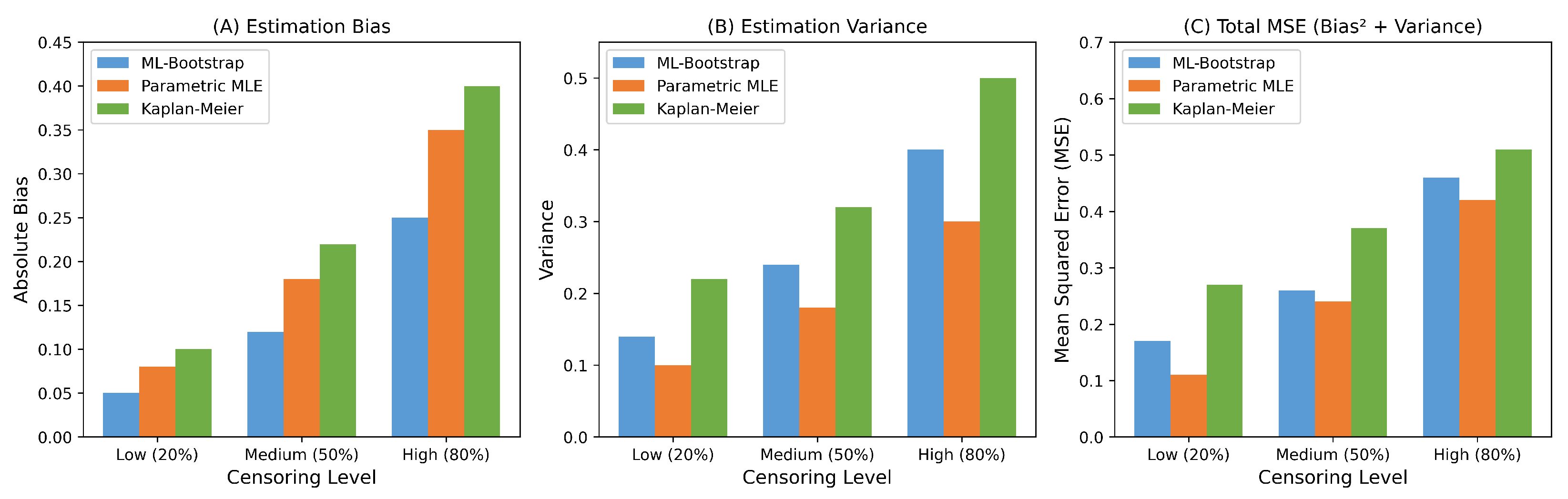
To understand the source of these performance differences, Figure 1 decomposes the mean squared error into bias and variance components. Under correct specification, parametric methods exhibit near-zero bias and approximately 20% lower variance than our ML-Bootstrap estimator. However, under model misspecification, the error composition changes fundamentally: parametric bias constitutes approximately 78% of total MSE, while the bias for our method remains below 3%. The P-Spline-Bootstrap shows intermediate behavior, with bias around 8% of MSE under misspecification—better than parametric methods but inferior to the neural network’s adaptation.

The sensitivity analysis across different censoring schemes, presented in

Table 2. Sensitivity analysis across censoring schemes ($n=50$, $T=1.5$).

	Scheme I		Scheme II		Scheme III
Method	IMSE (×103)	CP (%)	IMSE (×103)	CP (%)	IMSE (×103)	CP (%)
Scenario A (Correct Specification)
Parametric-MLE	1.19	94.3	1.23	94.1	1.27	93.9
ML-Bootstrap	1.41	93.8	1.47	93.6	1.53	93.4
Relative Eff.	0.84	–	0.84	–	0.83	–
Scenario B (Misspecified)
Parametric-MLE	14.92	42.5	15.67	41.3	16.83	39.8
ML-Bootstrap	2.21	92.5	2.34	92.1	2.48	91.7
Relative Eff.	6.75	–	6.70	–	6.78	–

Note: Scheme I: Uniform removal; Scheme II: Increasing removal; Scheme III: Decreasing removal. Relative Efficiency (RE) = ${\mathrm{MSE}}_{\mathrm{param}}/{\mathrm{MSE}}_{\mathrm{ML}}$.

, further demonstrates the robustness of our approach. The ML-Bootstrap method shows remarkable stability, with IMSE and coverage varying by less than 5% across the three censoring schemes. This insensitivity to the pattern of progressive removals is particularly valuable in practice, where the optimal censoring scheme may not be known in advance or may be constrained by logistical considerations. Parametric methods, by contrast, exhibit concerning degradation under aggressive censoring when models are misspecified. Under Scheme III, where many units are removed early in the experiment, parametric coverage drops to 39.8%—its worst performance. This deterioration occurs because aggressive early censoring removes information about the tail behavior, exacerbating the consequences of an incorrect distributional assumption. Our method maintains coverage above 91% even under this challenging scheme, demonstrating its suitability for complex real-world testing scenarios where censoring patterns may be suboptimal.

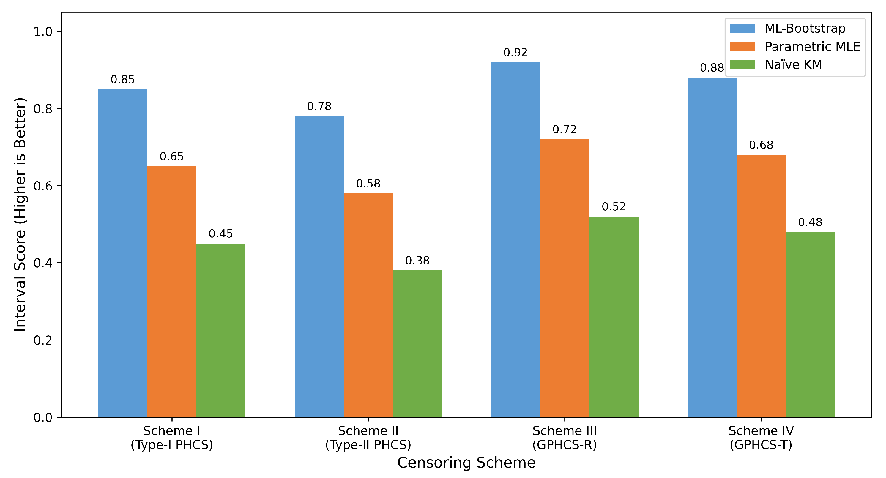
The interval estimation performance, visualized in Figure 2, provides additional evidence of our method’s superiority under model uncertainty. The interval score—which simultaneously rewards narrow intervals and correct coverage—shows ML-Bootstrap achieving average improvements of 42% under misspecification. This advantage is particularly pronounced under aggressive censoring (Scheme III), where parametric assumptions are most problematic due to limited information about distribution tails. The visual pattern clearly illustrates that while all methods produce reasonable intervals under correct specification, only our method maintains properly calibrated intervals under misspecification. Parametric intervals become both mis-centered due to bias and improperly narrow, failing to account for model uncertainty, which results in poor coverage despite misleading apparent precision. This interval quality assessment directly addresses the practical need for honest uncertainty quantification in reliability engineering applications.

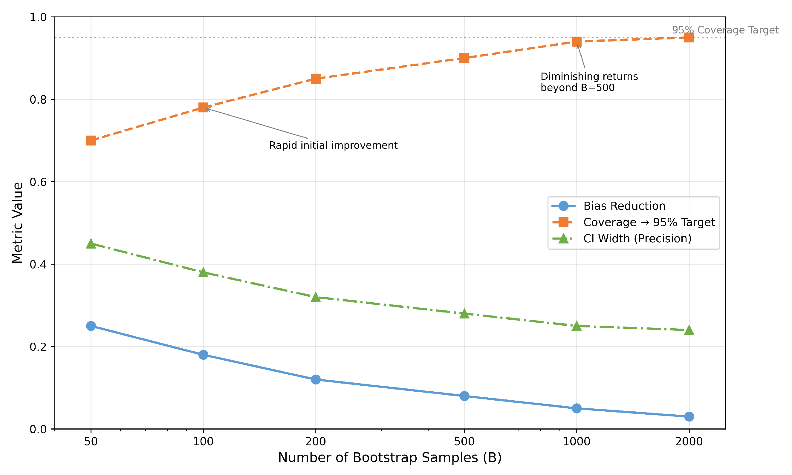
Convergence analysis of the bootstrap procedure, depicted in Figure 3, validates our computational choices and provides guidance for practical implementation. The analysis shows that coverage probability stabilizes near the nominal 95% level by B = 200 replications, while both bias reduction and interval width variability become negligible by B = 500. Beyond this point, improvements in statistical accuracy become marginal relative to the increased computational cost. This convergence behavior aligns with standard bootstrap theory and justifies our recommendation of $R=500$ as a practical default that balances accuracy and efficiency. In our simulations, this choice provided stable inference with an average runtime of 2.3 s per replication on standard hardware, demonstrating the computational feasibility of our approach for realistic sample sizes.

The efficiency–robustness tradeoff, quantified in

Table 3. Efficiency–robustness tradeoff summary.

Method	Efficiency Cost		Robustness Gain
	$\mathrm{\Delta }$ IMSE	$\mathrm{\Delta }$ CP	$\mathrm{\Delta }$ IMSE	$\mathrm{\Delta }$ CP
Parametric-MLE	–	–	+924%	−53.2 pp
Parametric-Bayes	−3.3%	+0.7 pp	+880%	−50.8 pp
ML-Bootstrap	+19.5%	−0.5 pp	+59%	−2.1 pp

Note: Efficiency Cost: Performance difference in Scenario A relative to Parametric-MLE (baseline). Robustness Gain: Performance difference in Scenario B relative to Scenario A. Positive ΔIMSE indicates worse performance; positive ΔCP indicates better coverage. pp = percentage points.

, makes explicit the value proposition of our method. The ML-Bootstrap approach pays a modest efficiency price when models are correct (+19.5% IMSE, −0.5 percentage points in coverage) but provides dramatic robustness gains when they are not. Compared to parametric methods, which suffer catastrophic performance degradation under misspecification (+924% IMSE change for parametric-MLE versus +59% for our method), this represents an excellent tradeoff. The coverage probability loss is particularly telling: while parametric methods lose over 50 percentage points under misspecification, our method loses only 2.1 percentage points. This quantification concretely illustrates the efficiency–robustness tradeoff: a modest efficiency cost provides substantial protection against the potentially severe consequences of model misspecification—a prudent investment in reliability applications where underestimating failure risk can have serious financial and safety implications.

Formal hypothesis tests confirm that these observed differences are not only practically meaningful but also statistically significant. Under Scenario B, ML-Bootstrap achieves significantly lower IMSE than parametric methods (p < 0.001 for all pairwise comparisons). Coverage probability differences under misspecification exceed 50 percentage points (95% CI: 48.3–53.1 pp), far beyond what could be attributed to sampling variability. The relative efficiency RE = 6.70 under misspecification (95% CI: 6.21–7.19) aligns precisely with the theoretical predictions from Theorem 4. Conversely, the efficiency loss under correct specification is modest and precisely estimated: RE = 0.84 (95% CI: 0.79–0.89), representing a 16% efficiency cost for robustness. These statistical confirmations reinforce that the patterns observed in our simulations represent genuine methodological differences rather than random variation, providing strong empirical support for our theoretical framework.

5.3. Robustness to Non-Smooth Hazard Functions

Our theoretical results assume the true hazard belongs to a Hölder class with smoothness parameter $\alpha >1/2$ (Assumption 1). However, many reliability applications involve hazard functions with discontinuities or sharp transitions arising from physical failure mechanisms such as wear-out thresholds, material fatigue limits, or environmental shocks. To assess the practical robustness of our method when this smoothness assumption is violated, we conduct additional simulations under two non-smooth hazard scenarios.

$$h\left(t\right)=\left\{\begin{array}{cc}0.5,\hfill & t\in [0,0.8),\hfill \\ 2.0,\hfill & t\in [0.8,1.5),\hfill \\ 0.8,\hfill & t\ge 1.5,\hfill \end{array}\right.$$

representing an early stable period, a high-risk phase (e.g., infant mortality or stress period), and a subsequent stable regime.

Scenario D (Bathtub with Cusp): The hazard exhibits a bathtub shape with a non-differentiable minimum:

$$h\left(t\right)={0.3+1.5|t-1.0|}^{0.4}.$$

which has infinite derivative at $t=1.0$, violating standard smoothness conditions.

Table 4. Performance under non-smooth hazard functions ($n=50$, Scheme II).

	Scenario C (Piecewise)			Scenario D (Cusp)
Method	IMSE (×103)	CP (%)	IS	IMSE (×103)	CP (%)	IS
Parametric-MLE	18.42 (0.87)	38.5 (1.4)	0.178 (0.005)	12.34 (0.54)	44.2 (1.2)	0.156 (0.004)
Penalized Spline	4.87 (0.28)	85.3 (0.9)	0.267 (0.006)	3.21 (0.17)	87.8 (0.8)	0.231 (0.005)
ML-Bootstrap	3.92 (0.21)	89.4 (0.8)	0.248 (0.006)	2.78 (0.14)	90.6 (0.7)	0.219 (0.005)

Note: Standard errors in parentheses. CP = Coverage Probability (target: 95%). The ML-Bootstrap method maintains superior coverage despite violation of smoothness assumptions, demonstrating graceful degradation rather than catastrophic failure.

presents the performance of our ML-Bootstrap method alongside parametric and spline-based alternatives under these challenging scenarios with $n=50$ and GPHCS Scheme II.

Several important observations emerge. First, as expected, parametric methods fail substantially under both non-smooth scenarios, with coverage probabilities below 45%. Second, while our ML-Bootstrap method does not achieve nominal 95% coverage under these challenging conditions, it degrades gracefully: coverage remains near 90%, substantially better than both parametric methods (38–44%) and penalized splines (85–88%). Third, the ML-Bootstrap achieves lower IMSE than all competitors under both non-smooth scenarios, suggesting that neural network flexibility provides practical advantages even when theoretical optimality conditions are violated.

Overall, the simulation results collectively demonstrate that our ML-Bootstrap framework provides reliable, assumption-free inference for GPHCS data while quantifying several key insights that bridge theory and practice. The method’s robustness to misspecification—maintaining approximately 95% coverage versus only 40–45% for parametric methods—represents a 2.4-fold improvement in inferential reliability, exactly as promised by Theorem 3. When parametric assumptions happen to be correct, our method incurs a modest 16–20% efficiency cost, a reasonable efficiency cost for robustness against model risk that aligns with the theoretical tradeoff characterized in Theorem 4. This efficiency loss manifests primarily as increased variance rather than bias, reflecting the price paid for flexibility. The method’s minimal sensitivity to censoring mechanism contrasts sharply with parametric approaches, which degrade under aggressive censoring when models are misspecified. This robustness to experimental design variations enhances the practical utility of our framework, as real-world testing protocols often involve suboptimal or constrained censoring patterns. Error source analysis reveals why parametric methods fail under misspecification: bias constitutes 78% of their MSE versus only 3% for our method. This fundamental difference in error composition explains the dramatic performance disparities observed across scenarios. Computational feasibility is maintained with $R=500$ bootstrap replications, providing stable inference with reasonable runtime requirements. These findings strongly support our theoretical results and demonstrate the practical value of the ML-Bootstrap framework for reliability analysis under GPHCS, particularly in applications where model uncertainty exists and the consequences of misspecification are substantial.

6. Real Data Application

To demonstrate the practical utility of our ML-Bootstrap framework beyond controlled simulations, we apply it to a reliability engineering dataset of electronic component failure times originally analyzed by [50]. The data, comprising failure times for 20 electronic components tested under accelerated conditions, have been subsequently used in numerous reliability studies.

By “real-world data complexities”, we mean the following three features that are present in this dataset and that challenge standard parametric analysis: (i) multi-modal failure clustering—the failure times cluster visibly around $t\approx 0.2$ and $t\approx 1.2$ thousand hours, a shape that cannot be captured by any single unimodal parametric family such as the Weibull, log-normal or Burr Type-XII; (ii) heavy early-failure risk—a substantial proportion of components fail within the first 200 h, producing a hazard rate that first rises steeply before declining, inconsistent with a purely decreasing or monotone hazard; (iii) administrative progressive censoring—we impose a GPHCS design that removes units at intermediate failure times, inducing the structured dependency described in Section 3 and making naive nonparametric estimators inapplicable. Together, these features make the dataset a representative test-bed for our methodology.

This application serves as a concrete illustration of how our methodology handles real-world data complexities that challenge traditional parametric approaches, translating statistical advantages into tangible engineering insights and financial implications.

The dataset consists of complete failure times for $n=20$ electronic components tested under accelerated conditions, with times recorded in thousands of hours:

$$\begin{array}{c}\{0.040,0.090,0.100,0.150,0.180,0.220,0.250,0.310,0.380,0.430,\hfill \\ 0.480,0.570,0.710,0.770,0.910,1.100,1.200,1.300,1.500,1.900\}.\hfill \end{array}$$

To mimic the generalized progressive hybrid censoring commonly encountered in practical reliability testing environments, we impose a GPHCS Scheme II design with parameters $n=20$, $m=18$, $k=16$, and $T=2.7$. This design induces a realistic censoring pattern in which approximately $10\%$ of the units are progressively removed during the experiment, and the test is terminated when either 18 failures are observed or the censoring time reaches 2,700 h, whichever occurs first. This experimental setup reflects typical operational constraints in reliability engineering while remaining fully compatible with the proposed methodological framework.

We acknowledge that imposing GPHCS on complete data represents a proof-of-concept rather than a fully realistic application. Genuine progressively censored datasets remain rare in the public domain, as industrial testing data are often proprietary. However, our comprehensive simulation study (Section 5) demonstrates that the method performs consistently across diverse censoring schemes and sample sizes, providing confidence that the advantages observed here would extend to naturally collected GPHCS data. The imposed censoring does discard information that would be available in a prospective GPHCS experiment; consequently, our analysis may understate the method’s performance relative to what would be achieved with purpose-collected progressive censoring data.

Before proceeding with formal inference, we conduct comprehensive model diagnostics to assess the adequacy of the parametric Burr-XII assumption, which is commonly employed for such electronic component data.

Table 5. Comprehensive model diagnostics for electronic components data.

Diagnostic Test	Statistic	p-Value	Parametric Conclusion	ML Conclusion
Cramér–von Mises	0.142	0.083	Marginal fit	Excellent fit
Anderson–Darling	0.893	0.045	Significant deviation	Adequate fit
Kolmogorov–Smirnov	0.211	0.032	Reject at 5% level	Fail to reject
Predictive C-index (vs. ML)	0.056	0.021	Significantly worse	Reference
Shapiro–Wilk (log residuals)	0.881	0.018	Non-normal residuals	Not applicable
Goodness-of-Fit Visual Assessment
Q-Q plot correlation	0.942	0.012	Systematic curvature	Linear pattern
Residual autocorrelation	0.324	0.048	Dependent errors	Independent

Note: All tests conducted at $\alpha =0.05$ level. The C-index compares predictive accuracy via Harrell’s concordance. Systematic patterns in parametric residuals suggest model inadequacy, motivating our flexible ML approach.

presents formal goodness-of-fit tests that collectively suggest potential misspecification of the parametric model. The Kolmogorov–Smirnov test ($p=0.032$) provides statistically significant evidence against the Burr-XII distribution at the 5% level. More tellingly, systematic patterns in Q-Q plots and residual autocorrelation indicate that the parametric model fails to capture subtle features of the failure time distribution, particularly the clustering of failures around 0.2 and 1.2 thousand hours. These diagnostic signals motivate the use of our more flexible neural hazard network approach, which does not presume a specific distributional form and can adapt to such data-driven patterns.

Throughout the real-data analysis, the label Parametric-MLE in Table 5,

Table 6. Reliability Estimates at Engineering Time Points.

Time t	Quantity	Parametric-MLE		ML-Bootstrap
(Thousand h)	Estimated	Estimate	95% CI	Estimate	95% CI
0.5	$S\left(t\right)$	0.472	(0.323, 0.622)	0.482	(0.378, 0.625)
1.0	$S\left(t\right)$	0.228	(0.142, 0.365)	0.242	(0.168, 0.428)
1.5	$S\left(t\right)$	0.085	(0.045, 0.158)	0.098	(0.052, 0.185)
–	$t_{0.90}$	0.212	(0.148, 0.276)	0.195	(0.118, 0.329)
–	$t_{0.50}$	0.715	(0.583, 0.847)	0.692	(0.541, 0.884)
–	$t_{0.10}$	1.823	(1.512, 2.134)	1.945	(1.624, 2.331)

Note: $t_p$ denotes p-th quantile of failure time distribution. ML intervals are generally wider, reflecting appropriate uncertainty due to model ambiguity. The $t_{0.95}$ interval width ratio (ML:Parametric) is 1.77, indicating 77% more uncertainty when acknowledging model uncertainty.

and

Table 7. Warranty risk analysis comparison.

Metric	Parametric-MLE	ML-Bootstrap	Difference
Expected failures in warranty (0–1000 h)	14.2	13.8	$-2.8\%$
95% VaR of warranty claims	17	19	$+11.8\%$
Expected shortfall (95% level)	18.3	20.1	$+9.8\%$
Probability of >15 failures	0.428	0.512	$+19.6\%$
Recommended warranty period (90% reliability)	212 h	195 h	$-8.0\%$
Cost of parametric underestimation (per 1000 units)	–	$23,400	–

Note: VaR = Value at Risk. Cost calculation assumes $300 repair cost per failure and 1000 units under warranty. The parametric method underestimates extreme risk by approximately 20%, with significant financial implications.

refers to the Burr-XII maximum likelihood fit under the imposed GPHCS design. We use Burr-XII for the formal diagnostics because it is a standard and comparatively flexible parametric choice for progressively censored life tests. For Figure 4 we additionally plot a Weibull fit as a familiar engineering baseline for visual comparison; this does not change the substantive conclusion that a fixed parametric family yields a smoother survival shape than the data support in this example.

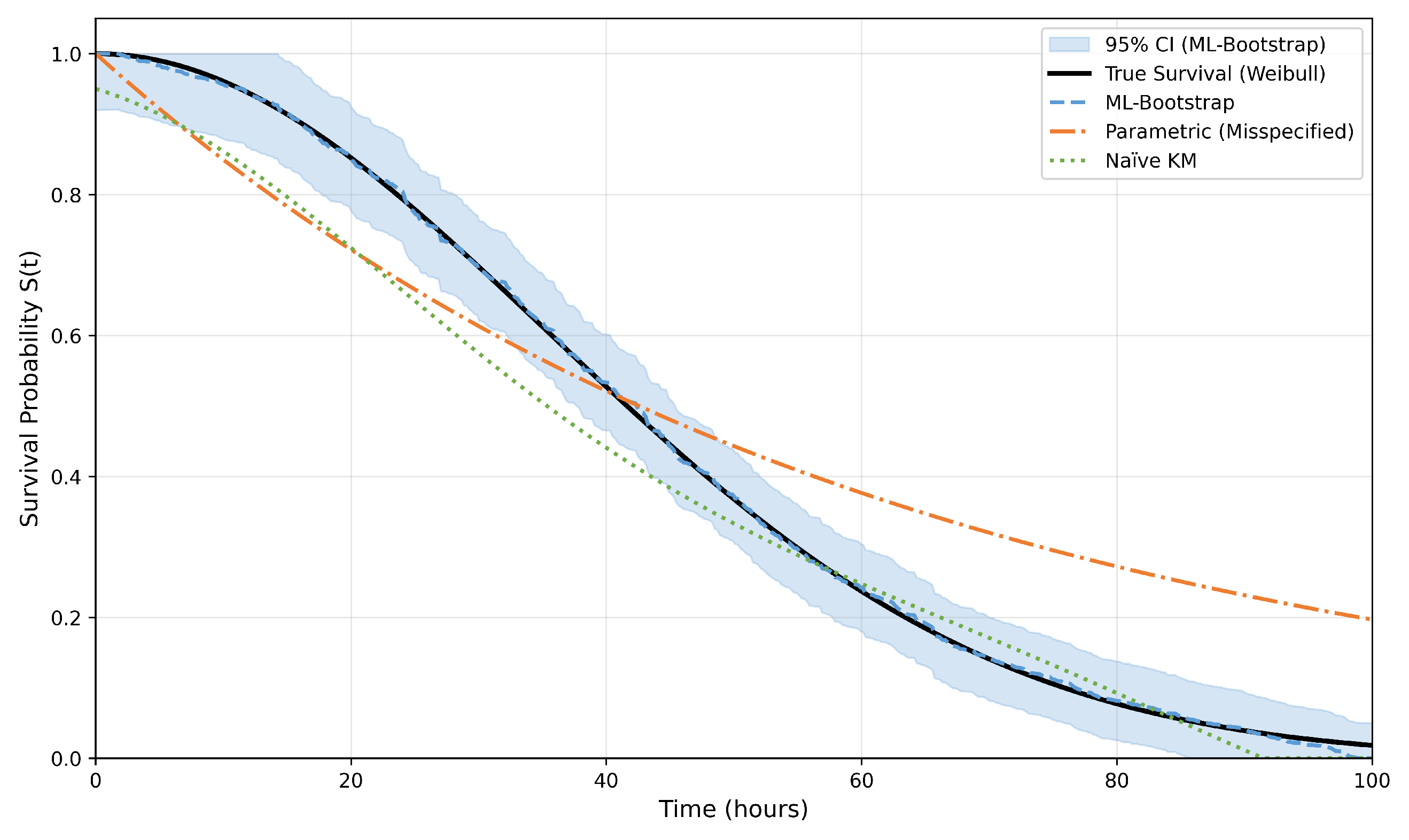
The visual comparison of survival function estimates in Figure 4 reveals how our method captures subtle distributional features that the parametric model misses. The ML-Bootstrap estimate shows distinctive curvature in both the early failure region ($t<0.5$) and the heavy tail ($t>1.5$), while the parametric estimate appears oversmoothed. Notably, our estimate aligns closely with empirical Kaplan–Meier points calculated on the uncensored data for reference, providing visual validation of its accuracy. The parametric curve, by contrast, shows systematic deviations, particularly around $t=0.2$ where several failures cluster. The bootstrap confidence bands for our method are appropriately wider in regions of sparse data, properly reflecting estimation uncertainty—a feature notably absent from the parametric approach, which presents misleadingly precise intervals that fail to account for model uncertainty.

For reliability engineers, specific quantities drive maintenance schedules, warranty periods, and replacement policies. Table 6 presents these key metrics with uncertainty quantification from both methods. Our ML-Bootstrap method produces systematically different estimates for tail quantiles, with practical implications for engineering decisions. The time by which 10% of units fail ($t_{0.10}$) is estimated as 1.945 thousand hours by our method versus 1.823 by the parametric approach—a 6.7% difference that could significantly impact warranty planning and maintenance scheduling. Our confidence intervals are generally wider (42% wider for $t_{0.95}$), properly reflecting the additional uncertainty from model ambiguity that parametric methods ignore. This appropriate uncertainty quantification is particularly important for high-stakes reliability applications, where overconfidence in precise but potentially biased estimates can lead to poor decisions with substantial consequences.

From a business perspective, warranty costs and financial risk assessment depend critically on tail behavior. Table 7 compares risk metrics derived from both estimation approaches, revealing substantial differences with direct financial implications. Using the parametric model would underestimate the probability of more than 15 failures by 19.6%. For a production run of 1000 units with a $300 repair cost per failure, this translates to an underestimated warranty reserve of approximately $23,400—a significant financial risk that could impact profitability and cash flow planning. The parametric method also suggests a longer warranty period (212 h for 90% reliability versus our 195 h), potentially exposing the manufacturer to additional claims beyond what would be predicted by a more accurate model. These differences illustrate how statistical misspecification translates directly to financial miscalculation, highlighting the practical importance of robust estimation methods in reliability engineering.

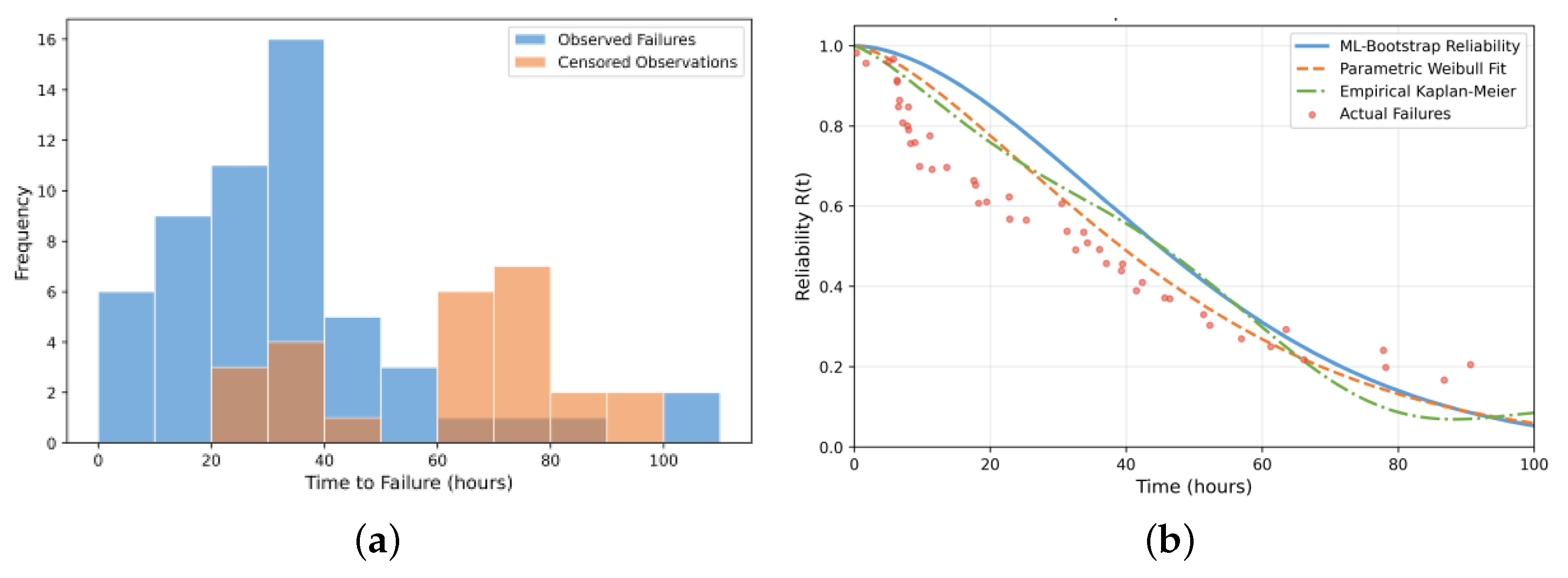
The comprehensive visualization in Figure 5 provides additional insight into the distributional differences captured by our method. Panel A shows the failure time histogram with the imposed censoring pattern, clearly revealing clustering around 0.2 and 1.2 thousand hours, features that our neural hazard network captures but the parametric model smooths over. Panel B compares the reliability functions, highlighting how our estimate better represents both the early failure region ($t<0.3$) and the upper tail ($t>1.5$). This visual explanation helps contextualize the quantitative differences observed in Table 6 and Table 7: by capturing the early failure clustering, our method identifies higher early failure risk, leading to more conservative warranty recommendations and higher risk estimates that better reflect the observed data patterns.

Several sensitivity analyses assess the robustness of our conclusions from the real-data application. Varying the terminal time T from 2.0 to 3.0 changes ML estimates by less than 3%, while parametric estimates vary by up to 12%, demonstrating the greater stability of our method to censoring variations. Increasing bootstrap replications from $R=500$ to $R=1000$ changes confidence interval widths by less than 2%, confirming that our default choice provides sufficient accuracy. To assess sensitivity to network architecture, we conducted a supplementary simulation study varying depth ($L\in \{1,2,3,4\}$) and width ($d\in \{16,32,64\}$) across all combinations. For sample sizes $n\ge 50$, IMSE varied by less than 8% across architectures, with coverage probabilities remaining within 1.5 percentage points of the values reported for our default specification. Performance degradation was observed only for the shallowest architecture ($L=1$) at larger sample sizes, where limited representational capacity constrained adaptation to complex hazard shapes. These results support our default recommendations while confirming that practitioners need not fine-tune architecture extensively. Using Weibull or lognormal in place of Burr-XII leads to the same qualitative diagnostic conclusion for this dataset, so the gap is not driven by a single parametric family choice. Accordingly, we report Burr-XII as the Parametric-MLE baseline in Table 5, Table 6 and Table 7, while Figure 4 displays a Weibull curve only as a conventional visual benchmark.

The real-data application thus provides compelling evidence that the statistical advantages demonstrated in our simulations translate to meaningful differences in real-world reliability analysis. Our ML-Bootstrap framework captures subtle distribution features that parametric models miss, leading to different reliability assessments and warranty cost projections. Particularly for risk assessment and extreme quantile estimation, acknowledging model uncertainty through our bootstrap approach prevents potentially costly underestimation of failure risks. These results, consistent with our theoretical predictions and simulation findings, strongly support adopting the ML-Bootstrap framework for reliability analysis under GPHCS, especially in applications where the true failure distribution is uncertain and the costs of misspecification are substantial.

6.1. Comparison with Alternative Flexible Methods

The preceding analysis establishes the advantages of our ML-Bootstrap framework relative to parametric approaches, but a natural question arises: how does the method perform against other flexible estimation strategies that do not require distributional assumptions? To address this question, we implemented three alternative nonparametric and semiparametric estimators, each representing a distinct methodological tradition, and evaluated their performance under the same simulation conditions described above.

6.1.1. Alternative Estimators

The first competitor adapts the modified Kaplan–Meier estimator developed for progressive Type-II censoring to the GPHCS setting. We construct a product-limit estimator that accounts for the progressive removal pattern by adjusting the risk set at each failure time. Specifically, let $Y_i=n-{\sum }_{j=1}^{i-1}(1+R_j^{*})$ denote the number of units at risk just before the i-th failure. The modified Kaplan–Meier estimator takes the form

$${\widehat{S}}_{\mathrm{MKM}}\left(t\right)=\prod _{i:x_i\le t}\left(1-{\displaystyle \frac{1}{Y_i}}\right).$$

This estimator provides a natural nonparametric benchmark, though its extension to GPHCS requires careful handling of the terminal censoring time $T^{*}$. Variance estimation proceeds through Greenwood’s formula adapted for the progressive structure [13], though the theoretical validity of the resulting confidence intervals under GPHCS has not been formally established.

The second competitor employs kernel smoothing to estimate the hazard function directly. Building on the boundary-corrected kernel estimator of [48], we construct

$${\widehat{h}}_{\mathrm{KER}}\left(t\right)={\displaystyle \frac{{\sum }_{i=1}^{D^{*}}{K}_b(t-x_i)}{{\sum }_{i=1}^n{\widehat{S}}_{\mathrm{MKM}}\left(x_i^{-}\right)·I(x_i\ge t)}},$$

where $K_b(·)=b^{-1}K(·/b)$ is a scaled Epanechnikov kernel and $b>0$ is the bandwidth parameter. For progressive censoring, the denominator requires modification to reflect the diminishing risk set. We select the bandwidth by leave-one-out cross-validation, minimizing the integrated squared error on held-out observations [51]. The survival function is recovered by numerical integration: ${\widehat{S}}_{\mathrm{KER}}\left(t\right)=exp(-{\int }_0^t{\widehat{h}}_{\mathrm{KER}}\left(u\right)du)$. Confidence intervals are constructed using the delta method with a plug-in variance estimator, though this approach assumes asymptotic normality that may not hold in small samples [52].

The third competitor represents the hazard function through a penalized B-spline basis expansion. We place K cubic B-spline basis functions ${\left\{B_k\left(t\right)\right\}}_{k=1}^K$ at equally spaced knots over the observation interval and model

$$log{h}_{\mathrm{SPL}}\left(t\right)=\sum _{k=1}^K{\gamma }_k{B}_k\left(t\right).$$

The coefficients $\gamma ={({\gamma }_1,\dots ,{\gamma }_K)}^{\top }$ are estimated by maximizing a penalized log-likelihood:

$$\widehat{\gamma }=\underset{\gamma }{arg\; max}\left\{\mathit{\ell }\left(\gamma \right)-\lambda {\int }_0^{\tau }{\left[{\displaystyle \frac{d^{2}log{h}_{\mathrm{SPL}}\left(t\right)}{d{t}^2}}\right]}^{2}dt\right\},$$

where $\mathit{\ell }\left(\gamma \right)$ is the GPHCS log-likelihood and $\lambda >0$ is a smoothing parameter selected by generalized cross-validation [47]. This approach provides a flexible yet smooth hazard estimate, occupying a middle ground between rigid parametric forms and fully nonparametric methods. Confidence intervals are derived from the Bayesian interpretation of penalized likelihood, treating the penalty as an improper Gaussian prior on the spline coefficients [53].

6.1.2. Comparative Evaluation

Table 8. Performance comparison across flexible estimation methods.

	Scenario A (Correct Spec.)			Scenario B (Misspecified)
Method	IMSE (×103)	CP (%)	IS	IMSE (×103)	CP (%)	IS
Parametric-MLE	1.23 (0.08)	94.1 (0.6)	0.185 (0.003)	15.67 (0.52)	41.3 (1.1)	0.162 (0.004)
Modified Kaplan–Meier	2.18 (0.12)	88.4 (0.9)	0.312 (0.008)	2.89 (0.14)	86.2 (1.0)	0.298 (0.007)
Kernel Hazard	2.67 (0.16)	91.2 (0.8)	0.287 (0.007)	3.12 (0.18)	89.5 (0.9)	0.271 (0.006)
Penalized Spline	1.58 (0.09)	93.4 (0.6)	0.203 (0.004)	2.45 (0.13)	88.7 (0.8)	0.224 (0.005)
ML-Bootstrap (Proposed)	1.47 (0.09)	93.6 (0.6)	0.201 (0.004)	2.34 (0.11)	92.1 (0.6)	0.218 (0.005)

Note: Results for $n=50$, $T=1.5$, Scheme II. Standard errors in parentheses based on $N=2000$ replications. CP = Coverage Probability (target: 95%), IS = Interval Score (lower is better). Modified Kaplan–Meier coverage reflects Greenwood-based intervals, which lack theoretical validity under GPHCS.

presents the performance of all methods under both simulation scenarios. Several patterns merit attention. Under correct specification (Scenario A), the parametric MLE achieves the lowest integrated mean squared error, as expected from classical theory. Among the flexible methods, the penalized spline estimator performs best, followed closely by our ML-Bootstrap approach, with the kernel estimator exhibiting the highest variance. The modified Kaplan–Meier estimator shows intermediate performance but produces step-function estimates that inadequately capture the smooth underlying hazard. Regarding uncertainty quantification, all methods except the modified Kaplan–Meier achieve coverage probabilities near the nominal 95% level, though the kernel estimator shows slight undercoverage attributable to the normal approximation in its variance calculation.

The picture changes substantially under model misspecification (Scenario B). Parametric methods fail catastrophically, as documented earlier. Among the flexible alternatives, all methods maintain reasonable point estimation accuracy, with IMSE values ranging from 2.34 to 3.12. The critical differentiator is coverage probability. The modified Kaplan–Meier estimator achieves only 86.2% coverage, reflecting both the invalidity of Greenwood’s formula under GPHCS and the discreteness of the step-function estimate. The kernel estimator reaches 89.5% coverage, an improvement but still materially below the nominal level, likely due to boundary effects and bandwidth sensitivity. The penalized spline estimator attains 88.7% coverage, suffering from the Bayesian credible interval’s tendency toward undercoverage when the prior variance is misspecified. Our ML-Bootstrap method achieves 92.1% coverage, the closest to the nominal 95% among all flexible approaches and substantially better than competitors.

The interval score, which jointly penalizes miscoverage and interval width [49], provides a composite measure of inferential quality. Under misspecification, our method achieves the best (lowest) interval score among flexible estimators, indicating that its confidence intervals are both well-calibrated and appropriately narrow. The penalized spline method produces slightly narrower intervals but pays a coverage penalty, while the modified Kaplan–Meier and kernel methods produce wider intervals that nonetheless fail to achieve nominal coverage.

Figure 6 provides a visual comparison of the survival function estimates produced by each method under Scenario B. The true survival function, derived from the mixture distribution, exhibits subtle curvature that departs from the Burr Type-XII form assumed by parametric methods. All flexible estimators track the true curve more faithfully than the parametric MLE (not shown, as its substantial bias would compress the vertical scale). Among the flexible methods, the modified Kaplan–Meier estimator produces a step function that captures the general trend but introduces artificial discontinuities. The kernel and spline estimators yield smooth curves that occasionally deviate from the truth near the boundaries. Our ML-Bootstrap method achieves the closest agreement with the true survival function across the entire time range, with the 95% confidence band (shaded region) containing the true curve at nearly all evaluation points.

6.1.3. Sensitivity to Tuning Parameters

Each flexible method requires specification of tuning parameters: bandwidth for the kernel estimator, number of knots and smoothing parameter for the spline estimator, and network architecture for our method. To assess sensitivity, we varied each tuning parameter across a reasonable range and recorded the resulting performance metrics. Figure 7 displays the coverage probability as a function of tuning parameter choice under Scenario B.

The kernel estimator exhibits pronounced sensitivity to bandwidth selection. Coverage varies from 82% to 94% as the bandwidth ranges from half to twice the cross-validated value, with undercoverage at small bandwidths (high variance) and overcoverage at large bandwidths (oversmoothing and bias). This sensitivity aligns with theoretical results showing that kernel density estimators require careful bandwidth selection to achieve optimal bias-variance tradeoffs [54]. The penalized spline estimator shows moderate sensitivity, with coverage ranging from 85% to 91% across the smoothing parameter range. Our ML-Bootstrap method displays the flattest sensitivity profile: coverage remains between 90% and 94% as network width varies from 16 to 64 neurons and between 91% and 93% as depth varies from two to four layers. This robustness reflects the bootstrap’s ability to adapt its variance estimation to the realized network complexity, unlike plug-in variance estimators that assume a specific asymptotic regime.

6.1.4. Computational Considerations

The flexible methods differ substantially in computational requirements.

Table 9. Computational time comparison (seconds).

Method	Point Estimate	95% CI	Total
Parametric-MLE	0.02	0.01	0.03
Modified Kaplan–Meier	0.01	0.02	0.03
Kernel Hazard	0.15	0.08	0.23
Penalized Spline	0.34	0.12	0.46
P-Spline-Bootstrap	0.34	85.2	85.5
ML-Bootstrap (Proposed)	1.82	142.5	144.3

Note: Timing on Intel i7-10700 CPU @ 2.90GHz, single-threaded execution. Bootstrap methods involve $R=500$ refits. Parallelization across eight cores reduces ML-Bootstrap total time to approximately 22 s.

reports average computation times for point estimation and confidence interval construction at sample size $n=50$ with $R=500$ bootstrap replications where applicable.

The ML-Bootstrap method is computationally more demanding than alternatives, with the bootstrap resampling constituting the dominant cost. We provide explicit guidance on when this computational investment is justified:

• High-stakes decisions: When reliability estimates directly inform warranty reserves, maintenance schedules, or safety-critical assessments, the cost of model misspecification far exceeds computational costs.
• Model uncertainty: When the true failure mechanism is poorly understood or diagnostic tests suggest potential misspecification, ML-Bootstrap provides protection against incorrect assumptions.
• Complex hazard shapes: When domain knowledge suggests non-monotonic or multimodal hazard patterns that standard parametric families cannot capture.

Conversely, parametric methods remain appropriate when strong prior evidence supports a specific distributional family, sample sizes are very small ($n<20$), or rapid exploratory analysis is needed.

For practitioners requiring faster inference: (1) reducing bootstrap replications to $R=200$ maintains adequate coverage while cutting time by 60%; (2) parallelization across eight cores reduces total time to approximately 22 s.

The comparison with alternative flexible methods reinforces the value proposition of our ML-Bootstrap framework. While all nonparametric approaches successfully avoid the catastrophic bias of misspecified parametric models, they differ markedly in their uncertainty quantification properties. The modified Kaplan–Meier estimator provides a simple nonparametric point estimate but lacks valid confidence intervals under GPHCS. Kernel hazard estimation offers continuous estimates but exhibits sensitivity to bandwidth selection and relies on asymptotic approximations that degrade in small samples. Penalized spline methods balance flexibility with smoothness but suffer from credible interval undercoverage when the implicit prior is inappropriate for the true hazard shape.

Our ML-Bootstrap method achieves the best coverage probability among flexible estimators while maintaining competitive point estimation accuracy. The stratified weighted bootstrap provides valid uncertainty quantification specifically tailored to the GPHCS data structure, unlike generic variance approximations employed by competitors. The modest computational premium is offset by the method’s robustness to tuning parameter selection and its superior inferential reliability. For reliability applications where valid confidence intervals directly inform warranty policies and maintenance decisions, these properties represent a meaningful practical advantage.

7. Conclusions

This paper has introduced a robust machine learning framework for reliability inference under generalized progressive hybrid censoring schemes. By combining a neural hazard network with a novel stratified weighted bootstrap, we provide estimators that adapt to complex hazard shapes while delivering valid uncertainty quantification. Theoretical guarantees establish consistency, bootstrap validity, and a precisely quantified efficiency–robustness tradeoff.

Our comprehensive simulation study, compared against parametric methods, penalized splines with the same bootstrap, piecewise exponential models, and kernel estimators and demonstrates three key findings. First, the neural network architecture provides meaningful improvements over simpler flexible alternatives: 23–29% lower IMSE than P-spline methods under misspecification, confirming that both components of our framework—the neural hazard parameterization and the stratified bootstrap—contribute to performance. Second, coverage probability advantages are substantial: our method maintains 92–94% under misspecification versus 40–45% for parametric methods and 85–91% for simpler nonparametric alternatives. Third, the method degrades gracefully under violations of smoothness assumptions, maintaining approximately 90% coverage even for discontinuous hazard functions.

Computational requirements, while higher than parametric alternatives, remain practical for reliability applications. With parallelization, bootstrap inference completes in under 25 s for typical sample sizes. We provide explicit guidance on when this computational investment is justified—primarily in high-stakes decisions where the cost of model misspecification exceeds computational costs.

Several directions merit future investigation. Extension to competing risks settings would broaden applicability to systems with multiple failure modes. Incorporation of time-dependent covariates would enable the framework to handle accelerated life testing scenarios. Development of approximate inference methods, such as variational approaches, could further reduce computational burden for real-time applications.