New Mathematics for Computer Performance: Array Algebra and Cost Functions

Abstract

MoA (mathematics of arrays) is a theory of parallel operations on arrays that can describe all known algorithms in linear algebra, signal processing, and HPC because they are based on primitive recursion and array shapes. Mapping parallel algorithms to computer architectures remains more of an art than a science, and specific mathematical techniques are needed to provide a basis for performance evaluation at a level abstract enough to constitute an experimental science. In this paper we present a methodology for parallel code generation from MoA expressions. Then, we relate the MoA operators to the linear space of memory elements in computer architecture. Finally, we define a theory of execution costs that is based on classical operations research and is formally related to MoA-based parallel code generation. This constitutes a formalized and mechanizable approach to performance prediction, portability and optimization.

1. Introduction

The productivity of high-performance computing (HPC) is low due to complex and ever-evolving hardware architectures, compilers, and the general lack of performance predictability. Our work is at the intersection of an algebra of arrays and parallel code generation: an algebraic expression is given as algorithm description and parallel code should be automatically produced from one of its many algebraically equivalent forms. The choice of the best form should be based on a parallel performance model that estimates execution time based on the array expression’s shape and the target architecture’s parameters such as the number of threads, number of GPUs/nodes, etc.

We provide core elements of this methodology that were investigated in previous works, and then compare it to other approaches to HPC. New mathematical results include the formal semantics relating array expressions to flat memory space and the formal basis for the performance models. Our overall long-term goal is ambitious: to combine the productivity of no-programming with high and predictable performance. Previously obtained experimental evidence and the formal basis for the array algebra give a foundation for an automatic exploration of array-based algorithms for all target architectures as driven by the performance models.

2. Problem Statement and Related Work

Languages and libraries used for producing parallel code are based on diverse concepts that do not help to structure parallel code, but rather add to its complexity: APL [1] was declarative and array-centered but is no longer in use; FORTRAN [2] has been relatively stable but requires the addition of explicitly-parallel libraries like MPI; high-performance Fortran (HPF) [3] was an attempt at removing this limitation by adding a process-mapping concept to Fortran; C [4] remains a stable alternative to Fortran for this purpose but shares the same defects as the libraries it is extended with (MPI, etc.). The Message Passing Interface (MPI) [5] proposes a clear concept of local process and global operations, but its semantics are non-deterministic and its syntax scoping is completely orthogonal to the process structures, a defect that obscures the parallel meaning of even the simplest codes. At its core is an unbound global variable pid that identifies the local process number, yet is bound “outside” the main program. As a result, MPI-based programs contradict the most basic idea of software engineering, namely, the context-free grammar. OpenMP [6] only applies to shared-memory computing so does not cover the scopes of MPI or CUDA. CUDA [7] is GPU-specific and proprietary. Other libraries emerge regularly that are more or less general purpose, for example, OpenACC [8] uses annotations to target hybrid CPU–GPU architectures, while Pytorch [9] is specific to machine learning.

In principle, the existence of tools based on diverse concepts could be a good thing. They could allow the developer to define a parallel application from various angles. But, in the current state of languages and libraries, that is not the case: it is not various angles of the same algorithm that are covered but various interconnected parts of the same global algorithm. CUDA covers the part that executes on a given GPU, MPI the choregraphy of nodes, etc. The various tools are not unified in a single intelligible semantics framework, let alone have a common performance model. Parallel programming is in the dark ages.

One could argue that sequential programming languages are also constantly evolving: Fortran, Algol, C, Java, and Python have all been popular in different periods and propose various programming concepts. But they are all based on the well-proven concepts of sequential computing. The panorama of parallel programming languages and libraries is not converging on a single concept that can combine the simplicity of expression and predictable performance.

As complex as they are, all hardware structures have one fundamental feature in common: they are built from arrays of repeated elements—vector units, cores, nodes, execution units, etc. This observation is the basis of our proposal for array-based parallel programming.

We call (parallel) performance model, or cost model, any mathematical system that relates program execution time to input size, input shape, source code and/or algorithm structure, number of processing units, or machine architecture. In that sense, parallel complexity theory is an extremely coarse performance model, while Amdahl’s law, bulk-synchronous parallel computing (BSP) [10,11,12], and the roofline model [13] are performance models. Our approach intends to (a) generate efficient code from mathematical descriptions and (b) use a performance model that combines all the above parameters to ensure the best choice of target code, while predicting performance with small errors around 10–25% [14]. Existing models have the following drawbacks:

• BSP computing assumes that execution is a sequence of asynchronous parallel sets of traces, interleaved with global exchange and sychronization phases. It benchmarks the target architecture for speed, bandwidth, and global synchronization delay, and combines this information with the algorithm’s computation digraph to produce a reliable and extensible cost, i.e., computation time estimate. The flat parallel structure of BSP (parallel structures are not nested) made it unsuitable for mapping to hierarchical systems, such that it could only represent one-level multicore/multinode or a single GPU’s elements. But that restriction has been lifted with several multi-level versions of BSP [15,16,17]. The work of Loulergue, Matsuzaki et al. [18] has derived a class of BSP algorithms mathematically, but BSP’s main drawback remains that it assumes a flat parallel form of computation, which does not fit all architectures.
• The roofline model [13,19] is a performance analysis technique for parallel executions. It relates global memory-access intensity with computation Flops per second rate. It supports performance tuning by giving hints at what part of the source code is responsible for not reaching maximal Flop/s rate. But that is precisely its main defect: it is blind to any algorithm (as opposed to code-) optimization, such as blocking or Strassen-like matrix multiplication, that would reduce the total number of operations. Like BSP, the roofline model has been given a multi-level extension [20]. In summary, the roofline model is relevant and useful but without a concept of source program so it is useless for parallel software engineering.
• Another approach to parallel programming is polyhedral compilation [21] with its well-studied theory and practice tiling and mapping source code to virtual processors. Its properties are similar to those of the BSP model. The source code is modeled as a set of loop nests, so the model has an obvious link to software engineering, but the mapping to virtual processors is done without any cost model.

Having an explicit algebra like MoA ensures a more varied search space for the most efficient program. For example, symbolic transforms can reduce the number of multiplications (Strassen, Winograd, etc.) and also apply more limited sets of loop transformations like in polyhedric compilation. Minimal execution time can only diminish when the search space widens. Because our transforms are based on the shape of the arrays, and not their size or dataflow graph, the search space is not exponential in the size of the arrays.

We propose to convert a declarative form of algorithms to executable code while maximizing performance and making it predictable [2]. The source description uses our algebra of multi-dimensional arrays called A Mathematics of Arrays (MoA) [22,23,24,25,26,27,28].

In [14], we proposed a proof of concept and software architecture for the declarative programming approach. If coupled in a logically reliable way to a generative AI system, it will become a no-programming method for HPC. The C programs generated from MoA expressions in [14] contained no “compilation” overhead because of the minimalist subset C target language and the absence of pointers or indirections.

But the cost prediction that was used in [14], despite being faithful and scalable, was not mathematically connected to the MoA algebra. In this paper, we begin to address this gap by providing mathematical results.

This work unites concepts from algorithm design, parallel programming, and parallel architectures whose disconnected use led to a productivity crisis in HPC [29]:

“While functional portability across a diverse set of platforms is an important feature of portable frameworks, achieving performance portability often requires vendor and platform-specific optimizations. Achieving performance portability, therefore, comes at the expense of productivity.”

Our work is expected to cover all know algorithms that use arrays (matrices, tensors) in a primitive recursive manner (with a finite set of bounded loops whose bounds depend on the array shapes). As such, neural net inference and training naturally falls within its scope, as they manipulate arrays that represent layers [30]. Nevertheless, ML techniques that do not use arrays such as random forests [31] fall outside the scope of our work.

Advice to the Reader: Notations

Our paper uses several types of notations and it is essential not to confuse them:

1.

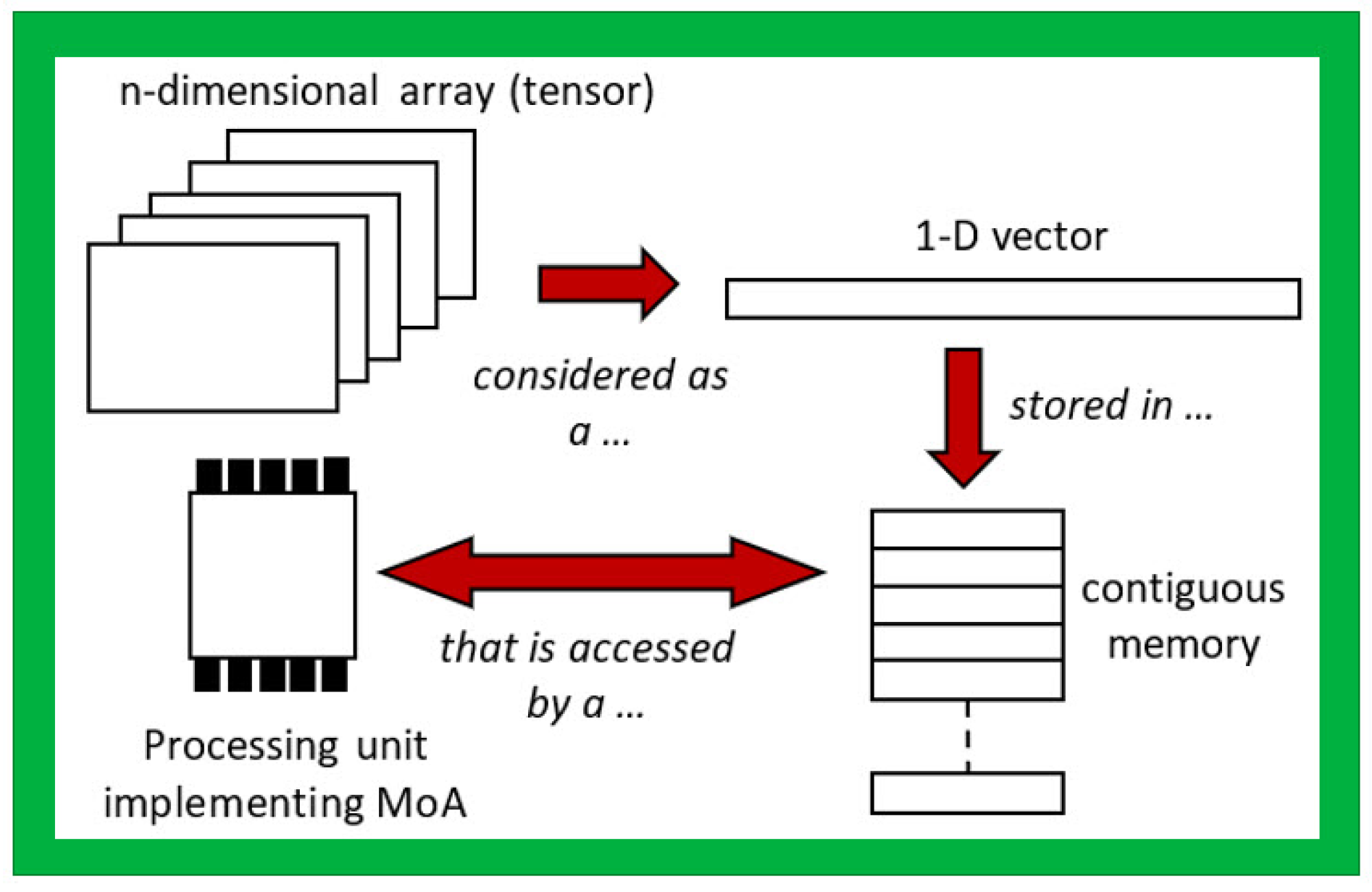
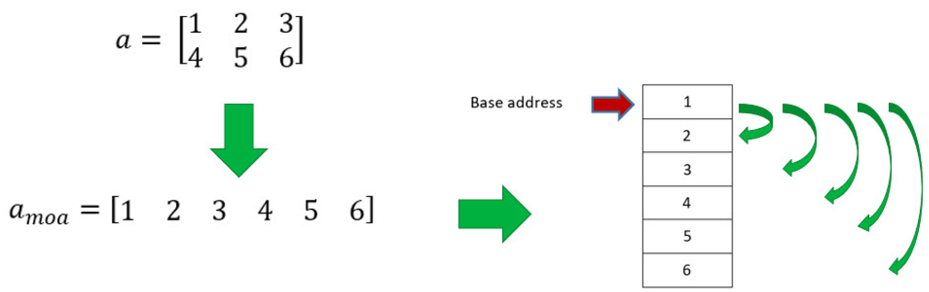
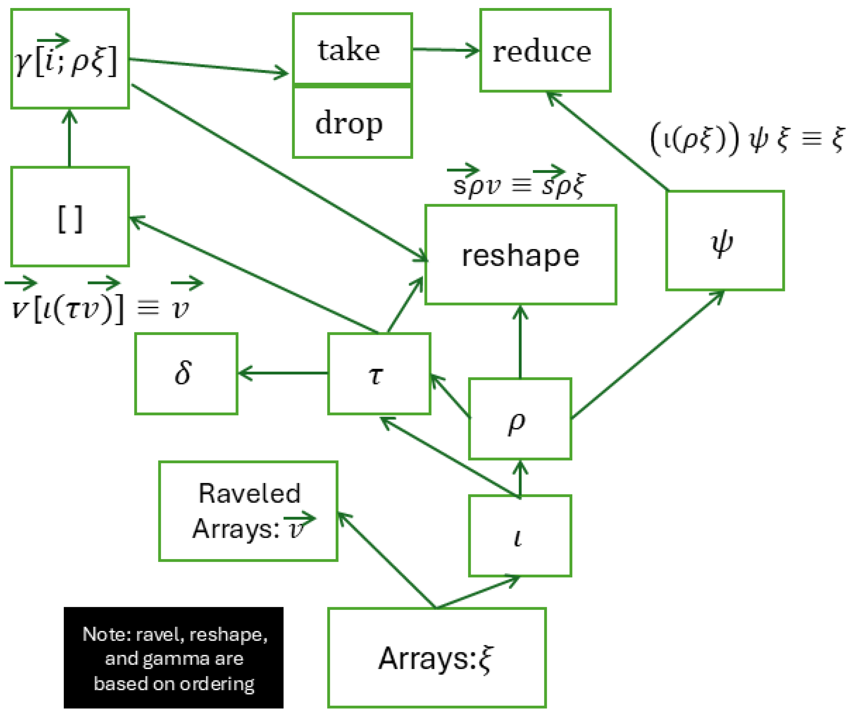
Section 3 uses MoA notation as it appears in many earlier papers. It can be used to model a great variety of array/tensor structures, operations on them (algorithms in declarative form), and directly or indirectly their mapping to machine structures that are themselves arrays. This style is that of usual applied mathematics, and operator semantics are implicit.

2.

Section 4 refers to a formal denotational semantics defined in an earlier paper and uses no special syntax, yet refers to the concepts of complete partial orders that justify the core intuition of MoA: a single type for all shapes and all dimensions of arrays.

3.

Section 5 defines and heavily uses operators on lists and pairs in a self-contained way. The expressions that relate to lists and pairs of lists give the operational semantics of MoA expressions. The MoA expressions that have those meanings are enclosed in double square brackets. For example, in $\left[\right|\xi \left|\right]=\left(\right[2,3,4],\kappa )$, $\xi$ is a variable that refers to an MoA array expression or constant, $\kappa$ is a variable whose value is some list of content values, and $[2,3,4]$ is a shape list that indicates the geometric shape of the array elements that $\kappa$ lists in lexicographic order. The reader not interested in symbolic computation, language semantics and programming language implementation may skip Section 5 but can refer to its explanation paragraphs after each definition to get a complete understanding of each MoA operator.

4.

Finally, Section 6 ignores operational semantics notation but uses two new notations: (a) program loop nests that are equivalent to normalized MoA expressions—reductions with indexings in flat arrays that implement the MoA reduction along certain dimensions; (b) costs associated to the loop nests, actually to the control-flow directed-acyclic graphs of those loop nests. As is classic in operations research, the costs have value in a semi-ring (e.g., max+ algebra). These notations have been chosen to justify such mathematical costs as an abstraction of measured execution time and/or memory consumption and/or energy consumption on real computers. Section 6 introduces the formal cost concept and justifies it as a (very incomplete but) formal exploration of a concept that is either implicit or absent from compilers and parallel programming libraries.

3. Mathematics of Arrays (MoA)

3.1. Principles of MoA

The idea of Mathematics of Arrays (MoA) considers the processing of data stored in multi-dimensional arrays (n-D arrays) by modeling the data array as a vector (1-D array). The mathematical operations (add/subtract, multiply/divide) then manipulate the data by considering the indexing of the elements within the vector, as depicted in Figure 1. Here, the n-D array (a tensor) is flattened so that the data is stored in contiguous memory that is then accessed by the suitable PU that performs the memory access and computation operations.

Consider a small example shown in Figure 2 to illustrate how MoA considers multi-dimensional arrays, where the dimension can be any dimension required.

Here, a 2 × 3 matrix holds integer values 1, 2, 3, 4, 5, 6. This will be defined in software, for example, in C:

$$\mathtt{int} \mathtt{example}\left[\mathtt{2}\right]\left[\mathtt{3}\right]=\left\{\right\{\mathtt{1},\mathtt{2},\mathtt{3}\},\{\mathtt{4},\mathtt{5},\mathtt{6}\left\}\right\};$$

3.2. MoA: The Basics

Mathematically, the idea of MoA, and Psi Calculus, starts with a scalar $\sigma$ and its shape $\rho \sigma$, an empty vector, denoted by $<>$ or $\Theta$. Since a vector is an array, it has a shape, $(\rho <>)\equiv <0>$, a one-element vector containing the integer 0, denoting that a scalar is a 0-dimensional array. Thus, from the shape, we can determine dimensionality, $\delta \sigma \equiv \left(\rho \right(\rho \sigma \left)\right)\left[0\right]\equiv <0>\left[0\right]\equiv 0$, and the total number of components, $\pi \left(\rho \sigma \right)\equiv \pi <>\equiv 1$, in the array. Algorithms on shapes describe how to index arrays with Psi and are defined, such that Psi takes a valid index vector, or an array of valid index vectors, and an array as arguments. For example, for a scalar, $\sigma$, $<>$, the empty vector, is the only valid index. Next, 2 scalars (0-D) and operations between them can be considered, with an extension to operations with n-dimensional (n-D) arguments.

Scalar operations are at the heart of computation, ${\sigma }_{l}f{\sigma }_r$, and, in general for n-d arrays, ${\xi }_{l}f{\xi }_r$, where f is an arbitrary scalar function. (When f is commutative, $\overrightarrow{i}\psi \left({\xi }_{l}f{\xi }_r\right)\equiv \overrightarrow{i}\psi \left({\xi }_{r}f{\xi }_l\right)$. In addition, if g is a scalar operation, $\overrightarrow{i}\psi \left({\xi }_{l_0}f\left({\xi }_{l_1}g{\xi }_r\right)\right)\equiv \overrightarrow{i}\psi \left(\left({\xi }_{l_0}f{\xi }_{l_1}\right)g{\xi }_r\right)$ and associative.)

Thus, in general,

$$\begin{array}{c}\forall \overrightarrow{i}\ni 0{\le }^{\ast }\overrightarrow{i}{<}^{\ast }\rho {\xi }_l\hfill \\ \hfill \hspace{1em}\hspace{1em}\hspace{1em}\hspace{1em} \overrightarrow{i}\psi \left({\xi }_{l}f{\xi }_r\right)\equiv \left(\overrightarrow{i}\psi {\xi }_l\right)f\left(\overrightarrow{i}\psi {\xi }_r\right)\end{array}$$

(1)

Here, $\overrightarrow{i}$ is a valid full index vector. That is, $\tau \overrightarrow{i}\equiv \delta \xi$. The ∗ notation denotes that all components of the index vector are within the bounds of its corresponding shape component:

That is, indexing distributes over scalar operations, or in compiler optimization terms, loop fusion.

For a scalar, there is only one valid index, $\overrightarrow{i}$ is $<>$, the empty vector.

$$<>\psi \left({\sigma }_{l}f{\sigma }_r\right)\equiv (<>\psi {\sigma }_l)f(<>\psi {\sigma }_r)$$

The equations above denote their Denotational Normal Form (DNF) and are in terms of cartesian coordinates.

$$\equiv \left(\mathrm{rav}{\sigma }_l\right)\left[{\gamma }_{row}(<>;<>)\right]f\left(\mathrm{rav}{\sigma }_r\right)\left[{\gamma }_{row}(<>;<>)\right]$$

Here we transform the DNF to its Operational Normal Form (ONF), or, to build the design, by flattening the array and relating that to offsets from the start of the array. ${\gamma }_{row}$ gets the offset using index and shape.

$$\equiv \left(\mathrm{rav}{\sigma }_l\right)\left[0\right]f\left(\mathrm{rav}{\sigma }_r\right)\left[0\right]$$

Here, the definition of ${\gamma }_{row}$ is applied in order to get 0.

$$\equiv (@{\sigma }_l+0)f(@{\sigma }_r+0)$$

This ONF now represents a generic form that uses bracket notation to denote how to build the code, through $\gamma$ and pseudo-code, i.e.,  $\mathrm{rav}\left(\overrightarrow{i}\psi \xi \right)\equiv \left(\mathrm{rav}\xi \right)\left[\gamma (\overrightarrow{i};\rho \xi )\right]$. With a family of gamma, $\gamma$, functions, e.g., row major(${\gamma }_{row}$), column major(${\gamma }_{column}$), a Cartesian index is related to an offset of the array in memory laid out contiguously. rav flattens an array based on its layout. Subscripts relate to left or right arguments and superscripts specify dimensionality. With this, introduce the important identify that is true in general for n-D arrays, denoted by $\xi$:

$$\left(\iota \right(\rho \xi \left)\right)\psi \xi )\equiv \xi$$

This means, with an array’s shape, $\rho \xi$, generate an array of indices, $\iota \left(\rho \xi \right)$. Then, using that array as an argument to Psi, the original array ξ, is returned.

In the scalar case, where $\sigma$ denotes a scalar,

$$\left(\right(\iota \left(\rho \sigma \right)\left)\psi \sigma \right)\equiv \sigma$$

The shape of a scalar is the empty vector $<>$ and the only valid index of a scalar. is

$$(\iota <>)\psi \sigma \equiv \sigma$$

$$<>\psi \sigma \equiv \sigma$$

Thus, as long as we can get shapes, e.g., $\rho \xi$, we can get all indices from shapes, e.g., $\iota \left(\rho \xi \right))$. This is true in in general, no matter the dimensionality of the array, including scalars, a 0-dimensional array.

Now, building on scalar operations, and extending to scalar vector operations, scalar extension is introduced, later generalized as the outer product. This generalization is completed by adding reductions/contractions and, the inner product (defined using reduction and outer product). Mullin’s research connects these four ideas formulated mathematically in MoA: scalar operations, matrix multiplication (MM), Hadamard Product (HP), and the Kronecker Product (KP) using a single algorithm/circuit [32]. These designs were extended to blocked matrix–matrix multiplication by first formulating in MoA, then derived, built, and tested in C, proving its performance exceeds modern DGEMM libraries [33].

MoA defines all operations using shapes and the Psi indexing function. Hence, when operations are formulated in the MoA algebra, they can be reduced through Psi Reduction to a semantic/denotational normal form (DNF), i.e., Cartesian indices of all operations are composed. This is called Psi Calculus. Then, one of the mapping functions, e.g., ${\gamma }_{row}$, transforms an index to an offset in memory, the ONF, or building it with knowledge of data layout that capitalizes on starts, stops, and strides. Next, formulating dimension lifting, i.e., partitioning shapes, leads to mapping data to hardware [34]. Combined with Lambda Calculus, iteration, sequence, and control [22], a Turing complete paradigm is realized to reason about array computation in general. These fundamentals allow one to define and optimize programs in any domain that use the algebra and could be enhanced subsets of any language with arrays, e.g., Fortran [2], Python [35], or Julia. That is, when there is semantic equivalence across programming languages, soft or hard, automatic linear and multi-linear transformations are easily applied, proving correctness by construction. MoA is a Universal Algebra (UA) that can optimize all domain-specific languages that use arrays/tensors as their primary data structure.

3.3. Dense Array Processing

It is important to understand why MoA’s design of matrix multiplication is different than other designs. Although the arithmetic complexity is the same and the arithmetic is the same, it is the fact that all arrays are accessed contiguously that give MoA’s MM an edge in performance. That is, the IO (Input–Output) complexity is better than other algorithms. Even when other algorithms have a better arithmetic complexity, e.g., Strassen, the fact that contiguous access does not occur makes for poorer performance. Note, this is why the MoA MM outperforms standard libraries [33,36].

Moreover, MoA’s design can treat any dimensional operation in the same way by first flattening the arrays, in row or column major ordering, followed by the use of starts, stops, and strides. The MoA MM is also very general: it is a 2-dimensional version of the inner product that can also take any two scalar operations as functional inputs, e.g., and with or. In addition, the MoA circuit not only performs the matrix multiplication, it can perform the Kronecker and Hadamard Product [27]. The only thing that differentiates the execution of multiple algorithms is that different starts, stops, and strides are fed into the circuit. This has important power and space attributes, which are that one circuit can perform four different algorithms.

Contiguous memory access easily allows the breaking up of loops, or what MoA refers to as the dimension-lifting or reordering of the array by shape refactorization. When one loop is broken into two, it may be partitioned to more than one resource, e.g., more than one MoA circuit or vector registers versus scalar registers. This concept can easily be done for as many resources as desired in an implementation based on the size of the problem and/or the number of resources available. This concept was used to block matrices in [33,36], where each block was accessed contiguously in the L1 cache.

3.4. MoA Matrix Multiplication

The general matrix–matrix multiplication (GEMM) in MoA is a special case of the inner product for 2-D arrays (matrices). Define $\mathbf{A}$ as an $m\times n$ matrix, $\mathbf{B}$ as $n\times p$, and $\mathbf{C}$ as $m\times p$. Let the following notation denote the 2-D matrix multiplication:

$$\mathbf{C}=\mathbf{A}•\mathbf{B}$$

(2)

In MoA notation, the shapes are:

$$\begin{array}{ccc}\hfill \rho \mathbf{A}=\langle m,n\rangle & \rho \mathbf{B}=\langle n,p\rangle & \rho \mathbf{C}=\langle m,p\rangle \hfill \end{array}$$

(3)

Next, define the valid indices of the matrices:

$$\forall i,j,k\ni \begin{array}{c}\{0\le i<m0\le j<p0\le k<n\}\hfill \end{array}$$

(4)

$\mathbf{C}=\mathbf{A}•\mathbf{B}$ is defined by the MoA Psi expression, given the shapes above.

$$<i>\psi \mathbf{C}\equiv {+}_{red}(<i,k>\psi \mathbf{A}\times (<k>\psi B))$$

(5)

Equation (5) uses the general $\psi$ indexing operator and is the DNF of our GEMM expression. Once reduced to its DNF, ${\gamma }_{row}$ is applied, thus producing the MoA Operational Normal Form (ONF) for GEMM, given by the following “generic” program.

$$\begin{array}{c}\hfill \mathbf{C}[(i\times p)+j]:=\sum _{k=0}^{n-1}\mathbf{A}[(i\times n)+k]\times \mathbf{B}[(k\times p)+j]\end{array}$$

(6)

Equation (6) is the generic code for a sequential program in MoA. In each of the ith rows of the resultant array $\mathbf{C}$, each scalar–vector operation involving the column index j is independent of each other one. The ith row of $\mathbf{C}$ is contiguously filled in by the summation of scalar–vector multiplications involving each matrix element at the ith row and kth column of $\mathbf{A}$ (the scalar) with each kth row of $\mathbf{B}$ (the vector) obtained by accessing the arguments contiguously. A row-wise sum reduction is then applied over the k index to yield the final answer as the i-th row in $\mathbf{C}$. The design is parallel at every step:

1.

Parallel row operations;

2.

Each n parallel row operation is performing m parallel scalar–vector multiplications;

3.

All n operations can be summed in $logn$ steps (ideally);

4.

Everything is accessed contiguously.

3.4.1. Example: Consider Performing a 3 by 4 with a 4 by 3, 2-D Matrix Multiplication

Consider the following example with two matrices A and B.

$$\mathrm{Let}:A\equiv \left[\begin{array}{cccc}0& 1& 2& 3\\ 4& 5& 6& 7\\ 8& 9& 10& 11\end{array}\right]\mathrm{and}\mathrm{let}B\equiv \left[\begin{array}{ccc}12& 13& 14\\ 15& 16& 17\\ 18& 19& 20\\ 21& 22& 23\end{array}\right]$$

Then, the matrix multiplication $C\equiv A•B$ is performed in the following way. The first row of the result is filled in contiguously as follows, while noticing how the left and right matrices are accessed contiguously.

$$\begin{array}{cc}\hfill (<0>\psi C)& \equiv ({\sum }_{n=0}^3(<0,n>\psi A)\times (<n>\psi B))\end{array}$$

(7)

That is, the entire 0-th row of C is

$$\begin{array}{c}\hfill (0\times <12,13,14>)+(1\times <15,16,17>)+(2\times <18,19,20>)+(3\times <21,22,23>)\end{array}$$

All other rows are processed as follows. Note the parallelism in all operations. The resultant C array is a 3 by 3 array.

$$\begin{array}{cc}\hfill (<1>\psi C)& \equiv ({\sum }_{n=0}^3(<1,n>\psi A)\times (<n>\psi B))\end{array}$$

(8)

$$\begin{array}{cc}\hfill (<2>\psi C)& \equiv ({\sum }_{n=0}^3(<2,n>\psi A)\times (<n>\psi B))\end{array}$$

(9)

The result is the expected 3 by 3 matrix:

$$C\equiv \left[\begin{array}{ccc}114& 120& 126\\ 378& 400& 422\\ 642& 680& 718\end{array}\right]$$

Reduce:

In Mullin’s dissertation, operator $\pi$ was introduced and related to the mathematical notation ∏. This is again mentioned in the definition of reduction, which is now explained here for higher-dimensional arrays.

$$\forall i\mathrm{s}.\mathrm{t}.0\le i<\left(\rho \xi \right)\left[0\right]$$

Product reduction (or any scalar operation), over the primary axis, is defined as

$$\prod _{i=0}^{\left(\right(\rho \xi \left)\right[0\left]\right)-1}<i>\psi \xi$$

This can be defined this way due to definitions of scalar operations on whole arrays, thus extending the example of

$${}_{\times }red\overrightarrow{v}\equiv \prod _{i=0}^{(\left(\tau \overrightarrow{v}\right)-1)}\overrightarrow{v}\left[i\right]$$

This is important to relate a recursive definition to iteration, essential for an optimal implementation of theory.

• Reshape:

Mullin’s dissertation explained how to reshape an arbitrary array. The example given uses a row major ordering. However, $\gamma$ can reshape given any ordering, e.g., column major, or any other defined ordering. When implemented, it is only the shape portion of the array that is changed, leaving the linear representation of the array, e.g., row or column major ordering, unchanged. It is important to note that reshape maps an initial shape to a desired shape based on the layout of the data in memory. Ideally, the contiguity of memory access (costs are modeled in later sections) is best in row major order. But that mapping can be arbitrary, as long as there is a 1–1 correspondence from one shape to another and it can be defined by a gamma, $\gamma$, function.

Reshape defines dimension lifting, a phrase defined to explain how each component of the original array’s shape, after psi-reduction to its DNF, is partitioned. This partition is based on the sizes, speeds, etc., or whatever attributes the DNF is mapped to, given a set of architectural components. As each component is broken into equal parts, the original shape becomes reshaped.

3.4.2. Example

Once the new shape is discovered, i.e., the lifted shape that maps with costs to the chosen architectural components, what was an 8 by 16 array becomes a 2 by 4 by 2 by 8 array, given that the rows are broken up over 2 processors and the columns are fed to 2 cycles of vector registers with length 8. That is, $\forall 0{\le }^{\ast }<i,j>{<}^{\ast }<8,16>$ so $<i,j>\psi \xi$ becomes $\forall 0{\le }^{\ast }<i^{\prime },i^{\prime \prime },j^{\prime },j^{\prime \prime }>{<}^{\ast }<2,4,2,8>:<i^{\prime },i^{\prime \prime },j^{\prime },j^{\prime \prime }>\psi \xi$. Now, casts can be calculated given the array size and datatype of how the array is mapped.

In [14], we summarize an extensive set of experiments and their analysis of (a) the exploration of a space of reshapes with (b) performance prediction by benchmarking small instances of the resulting MoA expression, reliably predicted performance on large arrays, and ensured that the most efficient version of the algorithm is chosen. Execution speeds have varied by factors of 10 in those experiments. In the next section, we describe in great detail the semantics of all MoA operators, a specification for algebraic transformations that are correct in all limit cases and all dimensions. Then, we describe the mathematical basis for general performance models that are not ad hoc but mathematically derived from the MoA expressions. Both new results improve on our previous work and have not been defined elsewhere.

4. Denotational Semantics

The intuitive box-shaped notion of multidimensional arrays has been formalized by the notion of array domains [37]: denotational semantics for all essential operators of MoA. Array denotations are the finite Scott domains (algebraic, bounded-complete and directed-complete partial orders) of partial functions from a boxed-shaped set of indices to a given base type. The information partial order is the increasing number of defined base-type values from an array that would have all its values undefined. In this ordered structure, an array is greater than another one if its shape is greater or equal to that of the other one, and it is pointwise greater than its values, i.e., it contains coherently more information. Array domain theory validates the following aspects of MoA definitions:

• The shape of an array is part of its value and, for a given base-type A, there is an array type (domain) $A^{\square }$ that contains arrays of all shapes with elements from A.
• Arrays have box shapes and not random patterns of index positions. Given a random subset of index positions where a base-type value is defined, the smallest array defined by those values has the shape that is the least enclosing box.
• Shapes containing the value 1 are allowed, e.g., shape $<3,1,3>$ is a plane in dimensions x, z and shape $<3,3>$ is a plane in dimensions x, y. Therefore, as in Pytorch [9], a dimension of length 1 allows the alignment of a tensor of fewer dimensions with another one of more dimensions before combining them.
• Shapes containing 0 values are allowed; they generate the empty ideal as input set for the content map, i.e., an empty array. The shape is part of the array value (not its type), so empty $<2,0>$ is not the same shape as empty $<0>$: the first one is an empty plane in dimensions x, y while the other is an empty line in dimension x. In other words, one cannot concatenate $<0>$ with $<2,1>$ but can concatenate $<2,0>$ with $<2,1>$.

5. Operational Semantics

We now provide a more concrete basis semantic space for arrays and their operators. It is based on the notion that a linear ordering of the array values can serve as a relay between the logical space of indices (the denotational array domains) and the physical space of data layout in computer architectures. Most operational semantics definitions are less intuitive than the standard geometric intuition. This is because the content values are not in a box-shaped container but in a list. For example, in a 2-dimensional array (matrix), rows are blocks of the content list but columns are not. But those definitions have the distinct advantage of spelling out the data layout in memory.

An array’s operational meaning is a pair of two lists. The first list is the shape and the second one is the content, i.e., list of elements in lexicographic order. The meaning of an operator on arrays is then a transformation function on such pairs.

Definition 1 (Arrays (operational definition)).

Assume a non-empty set of values A. An array $\xi \in A^{\square }$ is a pair $(\xi .\rho ,\xi .\kappa )$, where $\xi .\rho :{\mathbf{N}}^{\ast }$, the shape, is a possibly empty list of non-negative integers, and $\xi .\kappa :A^{\ast }$, the content, is a list of values from A such that the product of the integers in the shape is the length of the content list $\prod (\xi .\rho )=|\xi .\kappa |$.

Arrays of the form $\left(\right[],[a\left]\right)$ are called scalars and are in one-to-one correspondence with elements of A. When any element of $\rho$ is 0, the array is said to be empty, being of the form $(\rho ,[\left]\right)$. An empty array is denoted $\Theta$ or ${\Theta }_{\rho }$ if its form matters (this can happen when defining a concatenation along a certain axis).

Remark 1. 

There is an infinite variety of empty arrays: any array whose shape contains a 0 is empty and is distinct from empty arrays having different shapes.

Remark 2. 

A scalar array $\left(\right[],[a\left]\right)$ is distinct from an array of size one with non-empty shape, e.g., $\left(\right[1,1],[a\left]\right)$. This is because the shape is part of the array’s value and not its type. A scalar cannot be concatenated, while a non-scalar array of size 1 can be.

An array’s shape defines a box-shaped set of indices and its content is given in lexicographic order w.r.t. those indices. For example, $\left(\right(2,3),[(0,0);(0,1);(0,2);(1,0);(1,1);(1,2)\left]\right)$ is the array of type $\left(\mathbf{N}\right)$ shape $(2,3)$ whose content is the list of the indices. The complete denotational meaning of arrays, including partial order, infinite limits and information continuous functions, is defined in [37]. For the purpose of HPC applications, it is sufficient to assume the usual correspondence between Definition 1 and the usual “logical” meaning of arrays as maps from index boxes to values. We call the above “flat” definition the operational semantics because it resembles computer memory and is convenient for defining mappings from data and operations to hardware elements. We call the “logical” meaning the denotational semantics because it uses standard domain theory [37] and better matches the application domains for which arrays are defined.

Definition 2 (Flat indexing).

Let ξ be an array of shape $\rho =[{\rho }_0;\dots ;{\rho }_{d-1}]$ and content κ. The index domain of ξ is the cartesian product $dom\left(\xi \right)={\Pi }_{i=0}^{d-1}\{0;\dots ;{\rho }_i-1\}$. An index of ξ is a vector $\overrightarrow{i}\in dom\left(\xi \right)$. The flat indexing of ξ by $\overrightarrow{i}=[i_0;\dots ;i_{d-1}]$ is the content element

$$\xi [i_0;\dots ;i_{d-1}]=\kappa [i_0\times ({\rho }_1\times \dots \times {\rho }_{d-1})+\dots +i_{d-1}]=\kappa \left[\sum _{a=0}^{d-1}(i_a\times {\Pi }_{b=a+1}^{d-1}{\rho }_b)\right]$$

• If $\xi =\Theta$, then $dom\left(\xi \right)=Ø$ and there exists no index $\overrightarrow{i}$ of ξ. In this case, $\Theta \left[\overrightarrow{i}\right]$ is not defined.
• Another example is $\left[\right|\xi \left|\right]=\left(\right[2,3,4],\kappa )$ and $\xi [1,2,2]=\kappa [1\times (3\times 4)+2\times 4+2]=$$\kappa \left[22\right]$.

The MoA algebra generalizes this indexing with the $\Psi$ operator, whose value is itself an array. The index argument of $\Psi$ is not restricted to be of the same length as the shape of the array argument.

The Array Algebra

We now give a formal development of the core of MoA following the dependencies shown in Figure 3. Our definitions take the form of an operational semantics $\left[\right|\_\left|\right]$, whose input is an expression of the MoA algebra and whose value is an operational semantics that uses the flat definition. The abbreviations table at the end of this article spells out precisely our notations and their informal meanings, and separates MoA operators from the auxiliary operations that are needed to define their semantics.

Definition 3 (MoA algebra).

MoA is a one-sorted concrete algebraic structure: its base-type of elements is abstract but the array operators themselves are not axiomatized but rather defined. All constants and variables are of array type, written $X^{\square }$, where X is either $\mathbf{N}$ or a pure set of base elements A. For applications to linear algebra, it is assumed that A is a field or at least a semi-ring (max-+ algebra) for graph algorithms. The only elementary operator that requires this information is the reduction or generalized sum: parallel implementations require that A should have an addition that is associative. All other function symbols represent transformers, so their types are of the form $A^{\square }\times ...\times A^{\square }\to A^{\square }$, and they put no constraint on the base type.

MoA’s constants are the empty arrays $\Theta ,{\Theta }_{\rho }$, and empty vector $<>={\Theta }_{<0>}$. There are scalar variables $\sigma ,a,\dots ,z$ and general array variables $\xi ,{\xi }^n,{\xi }_{\rho }$, etc. The function symbols of arity 1 or more are those in Figure 3. Symbol ρ is overloaded times. As a variable, it denotes a shape vector (one-dimensional array), or a shape list in the operational semantics. As a unary function symbol, it denotes the operation that takes an array and returns this shape vector (or shape list meaning). As a binary function symbol, it is called reshape and denotes an operation that takes a new shape, an array, and produces a new array modified by this new shape. The operational semantics $\left[\right|\_\left|\right]$ takes a syntactic element of MoA and maps it to an array or array transformation in the flat representation. Its input is an MoA expression and its output is the meaning, defined with usual mathematical operations in lists.

Operational semantics are defined below for each operator.

Remark 3. 

Array constructors and destructors are implicit. In practice, this means that a software tool or API implementing MoA has predefined array constants: input/output operations that import/export arrays to or from other data types and channels. The action of such operations is not part of MoA theory, as it is context-dependent and not necessary for defining parallel algorithms.

Definition 4 (The shape operator).

The shape operator $\rho \_$ is unary, of type $A^{\square }\to {\mathbf{N}}^{\square }$, and its operational meaning is given by

$${\displaystyle \frac{\left[\right|\xi \left|\right]=(\xi .{\rho }^{\prime },\xi .\kappa )|\xi .{\rho }^{\prime }|=n}{\left[\right|\rho \left(\xi \right)\left|\right]=(\left[n\right],\xi .{\rho }^{\prime })}}.$$

In other words, ρ returns a vector whose content is the shape of its argument. For example, if $\left[\right|\xi \left|\right]=\left(\right[2;2],[a;b;c;d\left]\right)$, then $\left|\right[2;2\left]\right|=2$; therefore, $\left[\right|\rho \left(\xi \right)\left|\right]=(\left[2\right],\xi .{\rho }^{\prime })=(\left[2\right],[2;2])$, which is usually written $<2;2>$ in vector (1-D arrays) MoA notation.

Operator $\delta$ is called “dimensionality” to avoid confusion with dimension sizes. It counts the number of dimensions, that is, the length of the shape of an array.

Definition 5 (The dimensionality operator).

The dimensionality operator $\delta \_$ is unary, of type $A^{\square }\to {\mathbf{N}}^{\square }$, and has meaning

$${\displaystyle \frac{\left[\right|\xi \left|\right]=(\xi .\rho ,\xi .\kappa )|\xi .\rho |=m}{\left[\right|\delta \left(\xi \right)\left|\right]=\left(\right[],[m\left]\right)}}.$$

Thus, δ returns a scalar whose value is the length of the shape or number of dimensions of its argument. For example, if $\left[\right|\xi \left|\right]=\left(\right[2;2],[a;b;c;d\left]\right)$ then $|\xi .\rho |=2$, then $\left[\right|\delta \left(\xi \right)\left|\right]=\left(\right[],[2\left]\right)$, which, in MoA notation, is the scalar $\sigma =2$.

Definition 6 (The (total) size operator).

The size operator $\tau \_$ is unary, of type $A^{\square }\to {\mathbf{N}}^{\square }$, and has meaning

$${\displaystyle \frac{\left[\right|\xi \left|\right]=(\xi .\rho ,\xi .\kappa )\Pi (\xi .\rho )=t}{\left[\right|\tau \left(\xi \right)\left|\right]=\left(\right[],[t\left]\right)}}.$$

Thus, τ returns a scalar whose value is the product of the shape elements, or size of the index domain, of its argument.

For example, if $\left[\right|\xi \left|\right]=\left(\right[2;2],[a;b;c;d\left]\right)$ then $\Pi (\xi .\rho )=4$, then $\left[\right|\tau \left(\xi \right)\left|\right]=\left(\right[],[4\left]\right)$, which is the scalar $\sigma =4$.

Remark 4. 

By the definition of arrays, the total size value is the length of the content list.

We give here the well-known definition of concatenation and map on finite lists.

Definition 7 (List concatenation).

List concatenation $\_++\_$ has type $A^{\ast }\times A^{\ast }\to A^{\ast }$, neutral element $[\_]$, and is defined by $[x_0;\dots ;x_{a-1}]++[y_0;\dots ;y_{b-1}]=[x_0;\dots ;x_{a-1};y_0;\dots ;y_{b-1}]$.

List concatenation is associative, so whenever A is non-empty, $(A^{\ast },++,[\_])$ is a monoid, and list-length is a homomorphism $A^{\ast }\to (\mathbf{N},+,0)$.

List concatenation has an analog for vectors (1-dimensional arrays).

Definition 8 (Vector concatenation).

Vector concatenation $\_++\_:A^{\square }\times A^{\square }\to A^{\square }$ is defined when both arguments are vectors.

$${\displaystyle \frac{\left[\right|\overrightarrow{u}\left|\right]=(\left[m\right],\overrightarrow{u}.\kappa )\left[\right|\overrightarrow{v}\left|\right]=(\left[n\right],\overrightarrow{v}.\kappa )}{\left[\right|\overrightarrow{u}++\overrightarrow{v}\left|\right]=([m+n],\overrightarrow{u}.\kappa ++\overrightarrow{v}.\kappa )}}$$

In other words, vector concatenation concatenates contents and adds lengths to produce a vector.

Vector concatenation is associative with the empty vector as left/right neutral element.

Definition 9 (List map).

List map ${\_}^{\ast }$ has type $(A\to B)\to (A^{\ast }\to B^{\ast })$ and is defined by $f^{\ast }\left[\right]=\left[\right]$ and $f^{\ast }(\left[a\right]++l)=\left[f\left(a\right)\right]++l$. $f^{\ast }$ is an endomorphism on the list monoid.

The semantics of the take (array) operation uses the following list prefix–suffix operation that is used for taking content.

Definition 10 (List-take, or “prefix-suffix”).

We define the list-take operation $\_\hspace{0.17em}\uparrow \hspace{0.17em}\_:\mathbf{Z}\hspace{0.17em}\times \hspace{0.17em}{A}^{\ast }\to A^{\ast }$. Assume κ is a list of length n and $s:\mathbf{Z}$, such that $\left|s\right|\le n$. When s equals 0, then $s\uparrow \kappa =\left[\right]$. When s is positive, $s\uparrow \kappa$ equals $\left[\kappa \right[0];\dots ;\kappa [s-1\left]\right]$ but, if s is negative, then it equals $\left[\kappa \right[n+s];\dots ;\kappa [n-1\left]\right]$.

When the right argument of take is an array $\xi$, operation $2\uparrow \xi$ is well-defined if $\xi$’s first dimension (the technical definition of array take, Definition 11, allows for a scalar right argument without “first” dimension) is at least of length 2. Let us suppose that $\xi$’s shape list is $[3;4;5]$. Then, $\xi$ is abstractly equivalent to a 3-list of arrays of shape $[4;5]$. Then, producing the value of $2\uparrow \xi$ is equivalent to taking the first two such sub-arrays to produce an array of shape list $[2;4;5]$. The operational semantics of the MoA take operation are defined below. It may seem less intuitive or complex than the above explanation using nested array, but it has enormous logical and computational advantages: (a) absence of nesting removes the use of pointers, shape verifications, and multiple types, (b) moreover, an implementation can translate the flat semantics directly and statically into hardware mapping information.

Definition 11 (The take operator).

The take operator $\_\hspace{0.17em}\uparrow \hspace{0.17em}\_$ is binary, of type ${\mathbf{Z}}^{\square }\times A^{\square }\to A^{\square }$. It is defined when its left argument is a scalar integer, its right argument is an array of dimensionality at least 1, and it has the following meaning:

$${\displaystyle \frac{\begin{array}{c}\left[\right|\sigma \left|\right]=\left(\right[],[s\left]\right);\left[\right|\xi \left|\right]=(\xi .\rho ,\xi .\kappa );|\xi .\rho |\ge 1;\\ 1\uparrow \xi .\rho =\left[n\right];\left|s\right|\le n;(1\downarrow \xi .\rho )={\rho }^{\prime };\Pi \left({\rho }^{\prime }\right)=m\end{array}}{\left[\right|\sigma \uparrow \xi \left|\right]=\left(\right[\left|s\right|]++{\rho }^{\prime },(s\times m)\uparrow (\xi .\kappa ))}}$$

In other words, a take expression is well-defined if the left argument σ is an integer scalar (s) whose absolute value is no greater than the product of the first dimension of the array. Its result is an array whose content is a list prefix (or suffix if $s<0$) of the argument’s content and the shape begins with s and ends with the tail of the original shape:

• For example, if $\sigma =2$ is the left argument of take and ξ is the right argument of an array $\left(\right[3;4;5],[\kappa \left[0\right];\dots ;\kappa \left[59\right]\left]\right)$, then the definition’s parameters are $s=2$, $n=\Pi \left(\right[3\left]\right)=3$, $s\le n$ is verified, ${\rho }^{\prime }=[4;5]$, $m=\Pi \left(\right[4;5\left]\right)=20$. Therefore, the result $\left[\right|\sigma \uparrow \xi \left|\right]$ has shape $\left[\right|s\left|\right]++{\rho }^{\prime }=\left[2\right]++[4;5]$ =$[2;4;5]$, and its content is $(s\times m)\uparrow (\xi .\kappa )=(2\times 20)\uparrow (\xi .\kappa )$ = $40\uparrow (\xi .\kappa )=\left[\kappa \right[0];\dots ;\kappa [39\left]\right]$—the content of the first two “virtual sub-arrays” of shape $[4;5]$.
• If the left scalar argument had been $\sigma =-2$, the shape of the result would be the same, and the content would have been $(-40)\uparrow (\xi .\kappa )$, i.e., the last two “virtual sub-arrays” of shape $[4;5]$.
• If the left scalar argument had been $\sigma =0$, the result’s shape would be $[0;4;5]$ and the content would be $0\uparrow (\xi .\kappa )=\left[\right]$, which defines ${\Theta }_{[0;4;5]}$.

The semantics of the drop (array) operation are symmetrically based on the following list suffix–prefix operation that is used for taking content.

Definition 12 (List drop, or “suffix-prefix”).

Assume κ is a list of length n and $s:\mathbf{Z}$ such that $\left|s\right|\le n$.

When $s\ge 0$, $s\downarrow \kappa =\left[\kappa \right[s];\dots ;\kappa [n-1\left]\right]$, while, if $s<0$, then $s\downarrow \kappa =\left[\kappa \right[0];\dots ;\kappa [n-1+s\left]\right]$.

The meaning of the drop operator is a mirror image of that of the take operator.

Definition 13 (The drop operator).

The drop operator $\_\hspace{0.17em}\downarrow \hspace{0.17em}\_$ is binary, of type ${\mathbf{Z}}^{\square }\times A^{\square }\to A^{\square }$. It is defined when its left argument is a scalar, its right argument is an array of dimensionality 1 or more, and it has the following meaning:

$${\displaystyle \frac{\begin{array}{c}\left[\right|\sigma \left|\right]=\left(\right[],[s\left]\right);\left[\right|\xi \left|\right]=(\xi .\rho ,\xi .\kappa );|\xi .\rho |\ge 1;\\ 1\uparrow \xi .\rho =\left[n\right];\left|s\right|\le n;(1\downarrow \xi .\rho )={\rho }^{\prime };\Pi \left({\rho }^{\prime }\right)=m\end{array}}{\left[\right|\sigma \downarrow \xi \left|\right]=\left(\right[n-\left|s\right|]++{\rho }^{\prime },(s\times m)\downarrow (\xi .\kappa ))}}$$

Therefore, a drop expression is well-defined if the left argument σ is an integer scalar (s) whose absolute value is no greater than the first dimension of the array argument. Its result is an array whose content is a list suffix (or prefix if $s<0$) of the argument’s content and the shape begins with $n-s$ and ends with the tail of the original shape.

The next definition is an index constructor $\iota$. We begin with its list version and use it to define the multi-dimensional MoA meaning in a manner similar to how list take was used to define array take.

Definition 14 (The list index generator).

Assume $n:\mathbf{N}$; then, $\iota :\mathbf{N}\to {\mathbf{N}}^{\ast }$ is defined as follows: $\iota 0=\left[\right]$ and $\iota (n+1)=\iota \left(n\right)++\left[n\right].$

For example, $\iota \left(3\right)=iota\left(2\right)++\left[2\right]$ $=\iota \left(1\right)++\left[1\right]++\left[2\right]=\dots =[0;1;2]$.

The MoA index generator produces an array of indices.

Definition 15 (The index generator).

The index generator $\iota \_$ is unary of type ${\mathbf{N}}^{\square }\to {\mathbf{N}}^{\square }$. It is defined when its argument is a scalar or a vector (of integers) and has the following meaning:

$${\displaystyle \frac{\left[\right|\sigma \left|\right]=\left(\right[],[n\left]\right)}{\left[\right|\iota \left(\sigma \right)\left|\right]=\left(\right[n],\iota (n\left)\right)}}{\displaystyle \frac{\left[\right|\xi \left|\right]=\left(\right[n],v)(\prod v)=0}{\left[\right|\iota \left(\xi \right)\left|\right]=\left(\right[0],[\left]\right)}}{\displaystyle \frac{\left[\right|\xi \left|\right]=(\left[n\right],v)(\prod v)\ge 1++\Pi \left({\iota }^{\ast }\left(v\right)\right)=\kappa }{\left[\right|\iota \left(\xi \right)\left|\right]=(v++[n],\kappa )}}$$

where ${\iota }^{\ast }\left(\rho \right)\in {\left({\mathbf{N}}^{\ast }\right)}^{\ast }$ is the mapping of the list-index generator on the list of integers ρ, $\Pi \left({\iota }^{\ast }\left(\rho \right)\right)$ is the cartesian product of those index lists, and finally $++\Pi \left({\iota }^{\ast }\left(\rho \right)\right)$ is the concatenation of all those indexing lists of equal length. The condition $(\prod v)\ge 1$ ensures none of the elements of v is zero. Consider the following examples:

• The rule for scalar arguments applies to $\iota (\sigma =3)$. The semantics of σ are $\left(\right[],[3\left]\right)$, so $\left[\right|\iota \left(\sigma \right)\left|\right]=\left(\right[3],\iota (3\left)\right)$, which is the vector $<0;1;2>$ in MoA notation. In summary, $\iota (\sigma =0)=<>$, $\iota (\sigma =1)=<0>$, $\iota (\sigma =2)=<0;1>$, etc.
• If the argument vector contains a 0, then the second rule applies, $\prod v=0$, and $\iota \left(\xi \right)$ is then the empty vector $<>$.
• If the argument is a vector, the third rule applies. Let us apply ι to the empty vector ${\Theta }_{\left[0\right]}=<>$, whose meaning is $\left(\right[0],[\left]\right)$. In the left part of the inference rule’s denominator, $\left(\right[n],v)=\left(\right[0],[\left]\right)$, so $n=0$ and $v=\left[\right]$. The right part is then $\kappa =++\Pi \left({\iota }^{\ast }\left(v\right)\right)=$ $++\Pi \left({\iota }^{\ast }\left(\left[\right]\right)\right)=$ $++\Pi \left(\right[\left]\right)=$ $++\left(\right[\left[\right]\left]\right)=\left[\right].$ The denominator then yields $\iota (<>)=(v++[n],\kappa )$ $=\left(\right[]++[0],[\left]\right)=\left(\right[0],[\left]\right)$, which is again the empty vector. So $\iota (<>)=<>$.
• As an example of the most general case (without zeros), assume $\xi =<3;4>$ and let us compute $\iota \left(\xi \right)$. The numerator of the second rule produces $n=2$, $v=[3;4]$ and $\kappa =++\Pi \left(\right[[0;1;2];[0;1;2;3]\left]\right)=$ $[0;0;0;1;0;2;0,3;1;0;\dots ;2;3]$, where every block of length 2 is a possible index for an array of shape $[3;4]$.
  The meaning of $\iota (<3;4>)$ is thus $(v++[n\left]\right),\kappa )=$ $\left(\right[3;4;2],[0;0;0;1;0;2;0,3;1;0;\dots ;2;3\left]\right)$. Intuitively, this corresponds to a 3 array of indices of length 2.

Next, we consider indexing. Flat indexing (Definition 2) $\xi [i_0;\dots ;i_{d-1}]$ has two defects. First, it only applies to index lists that are exactly d long, where d is the dimensionality of $\xi$. We generalize this by (a) giving the result an array type, not the base type, and (b) allowing shorter index vectors. Another, less obvious defect is that its definition uses enumeration lists $[i_0;\dots ;i_{d-1}]$ specific to a certain dimensionality d. We replace this semi-formal description by a binary indexing operator $\Psi$ whose arguments are arrays. Its left argument provides indices, possibly produced by $\iota$, and the right one provides content.

• General array indexing is built from the following auxiliary function.

Definition 16 (The one-integer indexing operator).

One-integer indexing is binary, of type $\_[\_]:A^{\square }\times \mathbf{N}\to A^{\square }$, and is well-defined when the array argument is non-empty and the integer argument is no greater than the length of the first dimension of its array argument:

$${\displaystyle \frac{\xi \ne \Theta \left[\right|\xi \left|\right]=(\xi .\rho ,\xi .\kappa )1\uparrow \xi .\rho =\left[n\right]0\le i<n\Pi (1\downarrow \xi .\rho )=m}{\left[\right|\xi \left[i\right]\left|\right]=(1\downarrow \xi .\rho ,m\uparrow ((i\ast m)\downarrow (\xi .\kappa )\left)\right)}}$$

• Scalar array arguments are not allowed; they are excluded by the $1\uparrow \xi .\rho =\left[n\right]$ hypothesis in the rule. Indeed, for a scalar $\xi =(\sigma =s)$, $\xi .\rho =\left[\right]$ and so $1\uparrow \xi .\rho$ is undefined. As a result, the variable n is also undefined, etc.
• If the array is 1-dimensional, i.e., a vector, then, by hypothesis $\xi \ne \Theta$, it is a non-empty vector $\xi =<x_0;\dots ;x_{n-1}>$. Then, $\xi .\rho =\left[n\right]$ so $1\uparrow (\xi .\rho )=\left[n\right]$, so the possible indices are $i=0;\dots ;i=n-1$. Also, $\Pi (1\downarrow \xi .\rho )=\Pi \left[\right]=1=m$, and the denominator of the inference rule yields an array of empty shape $1\downarrow \xi .\rho =\left[\right]$ and content $m\uparrow \left(\right(i\ast m)\downarrow (\xi .\kappa \left)\right))=$ $1\uparrow \left(\right(i\ast 1)\downarrow (\xi .\kappa \left)\right))=$ $1\uparrow (i\downarrow \left([x_0;\dots ;x_{n-1}]\right))=x_i$. As such, in this case, $\left[\right|\xi \left[i\right]\left|\right]$ is the scalar $(\sigma =x_i)$.
• Assume $\xi .\rho =[2;256;2]$, $\xi .\kappa =[x_0;\dots ;x_{1023}]$ and let us compute $\xi \left[i\right]$ for $i=0$. In the numerator of the inference rule, we have $1\uparrow \xi .\rho =\left[2\right]$ so $n=2$, and $0\le i<n$ is verified. Also, $\Pi (1\downarrow \xi .\rho )=\Pi [256;2]=512=m$. The denominator of the rule yields, for a value of $\xi \left[i\right]$, the shape $1\downarrow \xi .\rho =[256;2]$ and content $m\uparrow \left(\right(i\ast m)\downarrow (\xi .\kappa \left)\right)=$ $512\uparrow ((0\ast 512)\downarrow [x_0;\dots ;x_{1023}])=$ $512\uparrow \left([x_0;\dots ;x_{1023}]\right)=$ $[x_0;\dots ;x_{511}])=$, which is the first (0th) sub-array of shape $[256;2]$ in ξ.
• With the same array ξ, if the integer-indexing was $i=1$, the numerator would give $n=2$, and $0\le i<n$ still verified. $m=512$ would not change, and the denominator would yield the same shape of $[256;2]$ but content $512\uparrow \left(\right(1\ast 512)\downarrow (\xi .\kappa \left)\right)=$ $512\uparrow \left([x_{512};\dots ;x_{1023}]\right)=$ $[x_{512};\dots ;x_{1023}]$, i.e., the second (rank 1) sub-array of shape $[256;2]$ in ξ.

Definition 17 (The indexing operator).

The indexing operator $\_\Psi \_$ is binary of type ${\mathbf{N}}^{\square }\times A^{\square }\to A^{\square }$. It is defined when its left argument $\overrightarrow{i}$ is a vector no longer than the shape of its right argument ξ. If the left argument is empty, the operation is the identity.

$${\displaystyle \frac{\left[\right|\overrightarrow{i}\left|\right]=(\left[0\right],\left[\right])}{\left[\right|\overrightarrow{i}\Psi \xi \left|\right]=\xi }}$$

In summary, $(<>\Psi \_)$ is the identity function on arrays.

If the left argument is of length 1 or more, indexing produces a sub-array of ξ whose content is defined recursively by one-integer indexing:

$${\displaystyle \frac{ }{\overrightarrow{i}\Psi {\Theta }_{\rho }={\Theta }_{\rho }}}{\displaystyle \frac{\xi \ne \Theta 1\uparrow \overrightarrow{i}=<i>1\downarrow \overrightarrow{i}=\overrightarrow{j}\xi \left[i\right]={\xi }^{\prime }}{\left[\right|\overrightarrow{i}\Psi \xi \left|\right]=\overrightarrow{j}\Psi {\xi }^{\prime }}}$$

• An empty array argument to Ψ requires a special rule because one-integer indexing $\Theta \left[i\right]$ is not defined. Operation $\overrightarrow{i}\Psi$ is the identity in this case.
• Suppose the indexing vector is of length 1, as in $<i>\Psi \xi$. Then, $1\uparrow <i>=<i>$, $1\downarrow \overrightarrow{i}=<>$, $\xi \left[i\right]={\xi }^{\prime }$, and the inference rule gives $\left[\right|<i>\Psi \xi \left|\right]=<>\Psi \left(\xi \right[i\left]\right)$, which equals $\xi \left[i\right]$ by the first inference rule. Thus, $<i>\Psi \xi$ is the one-integer indexing $\xi \left[i\right]$.
• The general case for $\overrightarrow{i}\Psi \xi$ is when $\overrightarrow{i}=<i>++\overrightarrow{j}$. The second inference rule is then $\overrightarrow{i}\Psi \xi =\overrightarrow{j}\Psi \left(\xi \left[i\right]\right)$.
• For example, let ξ be a 3-dimensional array of shape $[5;5;2]$, content $[x_0;x_1;\dots ;x_{49}]$, and let us compute $<1;0>\Psi \xi$. The above rephrasing of rule 2 produces $<1;0>\Psi \xi =$ $<0>\Psi \left(\xi \right[1\left]\right)=$ $<>\Psi \left(\xi \right[1\left]\right)\left[0\right]$, which by the first rule is equal to $\left(\xi \right[1\left]\right)\left[0\right]$. Two applications of Definition 16 then give a result of shape $\left[2\right]$ and content
  $2\uparrow ((0\ast 2)\downarrow (10\uparrow ((1\ast 10)\downarrow [x_0;\dots ;x_{49}])))=$
  $2\uparrow \left((10\uparrow (10\downarrow [x_0;\dots ;x_{49}]))\right)=$
  $2\uparrow \left((10\uparrow [x_{10};\dots ;x_{49}])\right)=$$2\uparrow \left([x_{10};\dots ;x_{19}]\right)=[x_{10};x_{11}]$,
  i.e., the first sub-array of shape $\left[2\right]$ in the second sub-array of shape $[5;2]$ of the initial array.

A direct consequence of Definition 17 is that it distributes over index concatenation.

Proposition 1. 

If $\delta \left(\overrightarrow{u}\right)=\delta \left(\overrightarrow{v}\right)=1$, $\overrightarrow{u},\overrightarrow{v}:{\mathbf{N}}^{\square }$, and $\left(\tau \overrightarrow{u}\right)+\left(\tau \overrightarrow{v}\right)\le \delta \xi$, then

$$(\overrightarrow{u}++\overrightarrow{v})\Psi \xi =\overrightarrow{v}\Psi (\overrightarrow{u}\Psi \xi )$$

In other words, when all indexing operations are well-defined, $(\overrightarrow{u}++\overrightarrow{v})\Psi \_=(\overrightarrow{v}\Psi \_)\circ (\overrightarrow{u}\Psi \_)$. When $\overrightarrow{u}$ and $\overrightarrow{v}$ are both of length one; this property can be written $<i,j>\Psi A=<j>\Psi (<i>\Psi A).$

Mullin [28] has extended Definition 17 to a left argument with general shape. In that more general version of the theory, one can prove the general indexing theorem.

Theorem 1 (indexing).

$$\left(\iota \right(\rho \xi \left)\right)\Psi \xi =\xi$$

This states the following: when indexing an array $\xi$ with the index generator applied to the shape of $\xi$, one recovers $\xi$. In other words, $\iota \circ \rho$ is the left-inverse of $\Psi$.

The distinctive feature of MoA arrays is that they are monolithic and homogeneous. They have both a multi-dimensional shape and a unique content list. Flattening an array is the transformation that retains its content but collapses it to a 1-dimensional shape.

Definition 18 (The ravel or flatten operator).

The ravel operator $\mathtt{rav}\_$ is unary of type $A^{\square }\to A^{\square }$ and is defined by the following rule:

$${\displaystyle \frac{\left[\right|\xi \left|\right]=(\xi .\rho ,\xi .\kappa )}{\left[\right|\mathtt{rav}\left(\xi \right)\left|\right]=\left(\right[\Pi \xi .\rho ],\xi .\kappa )}}$$

• If $\xi =\Theta$ is an empty array, then by definition of empty array $\Pi \xi .\rho =0$, $\xi .\kappa =\left[\right]$, and the flattened array has meaning $\left(\right[0],[\left]\right)$. Therefore, $\mathtt{rav}\left({\Theta }_{\rho }\right)=<>$ the empty vector.
• If ξ is a scalar $(\sigma =s)$, then $\xi .\rho$ is the empty list whose product is 1, so the flattened array has meaning $\left(\right[1],[s\left]\right)$, i.e., the singleton vector $<s>$.
• If $\xi =<>$, then $\xi .\rho =\left[0\right]$, so $[\Pi \xi .\rho ]=\left[0\right]$, and the content is empty, so $\mathtt{rav}<>=<>$.
• If $\xi =<x_0;\dots ;x_{n-1}>$, then $\xi .\rho =\left[n\right]$, so $[\Pi \xi .\rho ]=\left[n\right]$, and the content is unchanged, so $\mathtt{rav}<x_0;\dots ;x_{n-1}>=<x_0;\dots ;x_{n-1}>$. In all cases, for a vector $\overrightarrow{v}$, $\mathtt{rav}\left(\overrightarrow{v}\right)=\overrightarrow{v}$.
• If ξ is a multi-dimensional array of shape $\xi .\rho =[n_0;\dots ;n_{d-1}]$, then $\mathtt{rav}\xi$ is the vector of shape $\left[{\Pi }_{i=0}^{d-1}\left(n_i\right)\right]$ and with the same content as ξ. In other words, its content is $[\xi .\kappa [0;\dots ;0];\xi .\kappa [0;\dots ;1];\dots \xi .\kappa [n_0-1;\dots ;n_{d-1}-1]]$ in lexicographic order.

The index conversion operator expresses the correspondence between indices of $\xi$ and indices of $\mathtt{rav}\left(\xi \right)$: $\gamma (\overrightarrow{i},\overrightarrow{j})$ is the position of element $\overrightarrow{i}$ in the content list of an array of shape $\overrightarrow{j}$.

Definition 19 (The index conversion operator (standard, row major order) $\gamma$).

The gamma operator $\gamma (\_,\_)$ is binary, has type ${\mathbf{N}}^{\square }\times {\mathbf{N}}^{\square }\to \mathbf{N}$, and is defined when both arguments are vectors of the same length. Its value is given by the following rules:

$${\displaystyle \frac{ }{\gamma (<>,<>)=0}}$$

$${\displaystyle \frac{\delta \left(\overrightarrow{i}\right)=\delta \left(\overrightarrow{j}\right)=1\tau \left(\overrightarrow{i}\right)=\tau \left(\overrightarrow{j}\right)((-1)\uparrow \overrightarrow{i})=<a>((-1)\uparrow \overrightarrow{j})=<b>}{\gamma (\overrightarrow{i},\overrightarrow{j})=a+b\times \gamma ((-1)\downarrow \overrightarrow{i},(-1)\downarrow \overrightarrow{j})}}$$

• For example, $\gamma (<a>,<b>)$ is computed by the second rule: $\tau (<a>)=\tau (<b>)=(\sigma =1)$, $(-1)\uparrow <a>=<a>$, $(-1)\uparrow <b>=<b>$, so
  $\gamma (<a>,<b>)=a+b\times \gamma \left(\right(-1)\downarrow <a>,(-1)\downarrow <b>)=$$\hspace{0.17em}a+b\times \gamma (<>,<>)$, which by the first rule gives $\gamma (<a>,<b>)=a+b\times 0=a$.
• In the general case, $\gamma (\_,\_)$ is computed with the second rule as recursive application and the first one as base case: $\gamma (<a_0;\dots ;a_{n-1}>,<b_0;\dots ;b_{n-1}>)=$
  $a_{n-1}+b_{n-1}\times \gamma (<a_0;\dots ;a_{n-2}>,<b_0;\dots ;b_{n-2}>)$.
• As a 3-dimensional example, let us compute $\gamma (<1;2;3>,<5;10;20>)=$
  $3+20\times \gamma (<1;2>,<5;10>)=$$3+20\times (2+10\times \gamma (<1>,<5>\left)\right)=$
  $3+20\times (2+10\times 1)=$$3+20\times 2+20\times 10\times 1=$
  $(1\times 10\times 20)+(2\times 20)+3$.
  This last form of the expression highlights the general property that $\gamma (<1;2;3>,<5;10;20>)$ is the flat rank of index $[1;2;3]$ in the content of an array of shape $[5;10;20]$, namely, element 3 of the sub-array 2 of shape $\left[20\right]$ in sub-array 1 of shape $[10;20]$.

Proposition 2. 

For any non-empty array ξ, if $\overrightarrow{i}$ is of the same length as $\rho \left(\xi \right)$ and $\overrightarrow{i}$ is a well-defined index for ξ (which implies that ξ is neither a scalar or empty array), then

$$\left(\mathtt{rav}\left(\xi \right)\right)\left[\gamma (\overrightarrow{i},\rho \left(\xi \right))\right]=\xi \left[\overrightarrow{i}\right].$$

Proof. 

First remark: the equation in Proposition 2 is not defined for $\xi =\Theta$ because by Definition 2, flat indexing $\Theta \left[\overrightarrow{i}\right]$ is never defined. This is why the empty array is excluded from the identity.

• Base case. Suppose now that $\xi$ is a scalar $(\sigma =s)$, i.e., has empty shape and singleton content $\left[s\right]$. Then, the only possible index for $\xi$ is the empty vector $<>$ and the sum in the right-hand side of Definition 2’s equation is empty, so it equals 0. $\kappa \left[0\right]$ is then the list $\left[s\right]$ at position 0, i.e., the base-type element s, that is, the right-hand side of Proposition 2’s equation. Let us compute the left-hand side now. Here, it is $\gamma (<>,<>)=0$ by the definition of $\gamma$. $\left[\right|\xi \left|\right]=\left(\right[],[s\left]\right)$, so $\left[\right|\mathtt{rav}\left(\xi \right)\left|\right]=$ $\left(\right[\Pi \left(\right[\left]\right)],[s\left]\right)=$ $\left(\right[1],[s\left]\right)$; in other words, $\mathtt{rav}\left(\xi \right)$ is the one-element vector $<s>$. Therefore, $\left(\mathtt{rav}\left(\xi \right)\right)\left[\gamma (\overrightarrow{i},\rho \left(\xi \right))\right]=$ $<s>\left[0\right]=s$ which confirms the identity.
• Induction hypothesis. Assume that Proposition 2 holds for arrays of dimensionality d.
• Suppose $\xi$’s shape is of length $d+1$, and $\left[\right|\xi \left|\right]=$$({\rho }^{\prime }++\left[n_d\right]\xi .\kappa )$ and $\overrightarrow{i}=\overrightarrow{j}++\left[i_d\right]$ where ${\rho }^{\prime }$ and $\overrightarrow{j}$ are both of length d with ${\rho }^{\prime }=[{\rho }_0;\dots ;{\rho }_{d-1}]$ and $\overrightarrow{j}=[j_0;\dots ;j_{d-1}]$.
• Induction step. The contents of $\mathtt{rav}\left(\xi \right)$ and $\xi$ are the same, so we only need to verify that both flat indexings are the same. The equations’ right flat indexing is $\left[\overrightarrow{i}\right]=$ $[j_0;\dots ;j_{d-1};i_d]$, and this is equal to $[{\sum }_{a=0}^{d-1}(j_a\times {\Pi }_{b=a+1}^{d-1}{\rho }_b)+i_d]$ by the definition of flat indexing.
• Meanwhile, the left (rav) indexing is $\gamma (\overrightarrow{i},\rho \left(\xi \right))=$ $\gamma ([j_0;\dots ;j_{d-1};i_d],[{\rho }_0;\dots ;{\rho }_{d-1};n_d])$. By the definition of $\gamma$, this is equal to $\gamma ([j_0;\dots ;j_{d-1}],[{\rho }_0;\dots ;{\rho }_{d-1}])\times n_d+i_d.$ By the induction hypothesis, we can assume that indexing $\left[\gamma ([j_0;\dots ;j_{d-1}],[{\rho }_0;\dots ;{\rho }_{d-1}])\right]$ is the same as indexing by $\overrightarrow{j}$, which is $[j_0;\dots ;j_{d-1}]$. By the definition of flat indexing, this is also $\left[{\sum }_{a=0}^{d-1}(j_a\times {\Pi }_{b=a+1}^{d-1}{\rho }_b)\right]$. As a result, the left indexing $\gamma ([j_0;\dots ;j_{d-1}],[{\rho }_0;\dots ;{\rho }_{d-1}])\times n_d+i_d$ equals
• $\left[{\sum }_{a=0}^{d-1}(j_a\times {\Pi }_{b=a+1}^{d-1}{\rho }_b)\right]\times n_d+i_d=$
• $\left[{\sum }_{a=0}^{d-1}(j_a\times {\Pi }_{b=a+1}^d{({\rho }^{\prime }++\left[n_d\right])}_b)\right]+i_d=$
• $\left[{\sum }_{a=0}^{d-1}(j_a\times {\Pi }_{b=a+1}^d{\rho }_b)\right]+i_d$.    □

The above definition of index conversion (Definition 19) is based on the so-called row major order of array elements. The name refers to the two-dimensional case (matrices) where the first index integer refers to rows and the second one to columns. There is also a column major order of array elements, generalizing the representation of matrices as vectors of columns, instead of vectors of rows. It represents cases where the hardware stores arrays with indices read right-to-left, and the corresponding index conversion function is the following.

Definition 20 (The index conversion operator (column major order) ${\gamma }_{col}$).

The column major gamma operator ${\gamma }_{col}(\_,\_)$ is binary, has type ${\mathbf{N}}^{\square }\times {\mathbf{N}}^{\square }\to \mathbf{N}$ and is defined when both arguments are vectors of the same length. Its value is defined by the following rules:

$${\displaystyle \frac{ }{{\gamma }_{col}(<>,<>)=0}}$$

$${\displaystyle \frac{\delta \left(\overrightarrow{i}\right)=\delta \left(\overrightarrow{j}\right)=1\tau \left(\overrightarrow{i}\right)=\tau \left(\overrightarrow{j}\right)1\uparrow \overrightarrow{i}=<a>1\uparrow \overrightarrow{j}=<b>}{{\gamma }_{col}(\overrightarrow{i},\overrightarrow{j})=a+b\times {\gamma }_{col}(1\downarrow \overrightarrow{i},1\downarrow \overrightarrow{j})}}$$

Reshaping transforms an array’s shape while retaining its content. It lies at the core of our methodology for mapping MoA expressions to parallel architectures.

Definition 21 (The reshape operator).

The reshape operator $\_\widehat{\rho }\_$ is binary, is of type ${\mathbf{N}}^{\square }\times A^{\square }\to A^{\square }$ and is well-defined when its left argument is a vector.

$${\displaystyle \frac{\xi \ne \Theta \mathtt{rav}\left(\xi \right)\left[0\right]=x}{\left[\right|<>\widehat{\rho }\xi \left|\right]=(\left[\right],x)}}$$

$${\displaystyle \frac{\begin{array}{c}\xi \ne \Theta \left[\right|\xi \left|\right]=(\xi .\rho ,\xi .\kappa )\delta \left({\rho }^{\prime }\right)=(\sigma =1)\Pi (\xi .\rho )=n\Pi \left({\rho }^{\prime }\right)=n^{\prime }\\ \forall i.(0\le i<n^{\prime }).x_i=\xi .\kappa [imodn]{\kappa }^{\prime }=[x_0;\dots ;x_{n^{\prime }-1}]\end{array}}{\left[\right|{\rho }^{\prime }\widehat{\rho }\xi \left|\right]=({\rho }^{\prime },{\kappa }^{\prime })}}$$

In other words, the result of reshaping by an empty vector produces a scalar whose value is the first element in the content of the array argument. This non-intuitive property is a necessary consequence of the semantics of MoA and the property that reshaping by ${\rho }^{\prime }$ produces an array of shape ${\rho }^{\prime }$. That property also holds for the general case, and the content of the reshaped array is either a prefix or an extension of the original content by cyclic repetition.

The next operator we define is core to all linear-algebra applications of arrays, namely, the reduction of the array for given binary operations. Reduction depends on the following auxiliary definition of scalar extension, namely, pointwise extension to arrays of a given scalar operation.

Definition 22 (Scalar (pointwise) extension).

The extension of a given operation on type A applies to arrays of $A^{\square }$ and operates on its elements pointwise.

$${\displaystyle \frac{\mathtt{uop}\_:A\to A\left[\right|\xi \left|\right]=(\xi .\rho ,\xi .\kappa )\xi .\kappa =[x_0;\dots ;x_{n-1}]{\kappa }^{\prime }=[\mathtt{uop}\left(x_0\right);\dots ;\mathtt{uop}\left(x_{n-1}\right)]}{\left[\right|\mathtt{uop}\left(\xi \right)\left|\right]=(\xi .\rho ,{\kappa }^{\prime })}}$$

$${\displaystyle \frac{\begin{array}{c}\_\mathtt{op}\_:A\times A\to A\left[\right|\xi \left|\right]=(\xi .\rho ,\xi .\kappa )\left[\right|{\xi }^{\prime }\left|\right]=({\xi }^{\prime }.\rho ,{\xi }^{\prime }.\kappa )\xi .\rho ={\xi }^{\prime }.\rho \\ \xi .\kappa =[x_0;\dots ;x_{n-1}]\xi .\kappa =[y_0;\dots ;y_{n-1}]\kappa \prime \prime =[\left(x_0\right)\mathtt{op}\left(y_0\right);\dots ;\left(x_{n-1}\right)\mathtt{op}\left(y_{n-1}\right)]\end{array}}{\left[\right|\left(\xi \right)\mathtt{op}\left({\xi }^{\prime }\right)\left|\right]=(\xi .\rho ,\kappa \prime \prime )}}$$

Both definitions apply to empty arrays and produce empty arrays: $\mathtt{uop}\left({\Theta }_{\rho }\right)=\left({\Theta }_{\rho }\right)$ and $\left({\Theta }_{\rho }\right)\mathtt{op}\left({\Theta }_{\rho }\right)=\left({\Theta }_{\rho }\right)$.

Definition 23 (The reduction operator).

Suppose an associative binary operation ⊕ on type A, having neutral element $id(\oplus )$, i.e., a monoid $(A,\oplus ,id(\oplus \left)\right)$. The reduction operator for arrays of $A^{\square }$, is of type

$${\mathtt{red}}_{\_}(\_):(A\times A\to A)\times A^{\square }\to A^{\square }$$

and is defined when its second argument, the array, has dimensionality 1 or more.

$${\displaystyle \frac{ }{{\mathtt{red}}_{\oplus }\left({\Theta }_{\rho }\right)=(1\downarrow \rho )\widehat{\rho }\left(id(\oplus )\right)}}$$

$${\displaystyle \frac{\tau \left(\rho \right)\ge 1\xi \ne \Theta }{{\mathtt{red}}_{\oplus }\left(\xi \right)=(<0>\Psi \xi )\oplus \left({\mathtt{red}}_{\oplus }(1\downarrow \xi )\right)}}$$

Notice: the central ${\mathtt{red}}_{\oplus }$ operation in the last rule’s denominator is a scalar extension to arrays.

Neutral elements are needed to apply the first rule. For example, if $(A,\oplus ,\mathrm{id}(\oplus \left)\right)$ is $(\mathbf{N}\cup \{\infty \},max,0)$, then $\mathrm{id}(\oplus )=0$. In $(\mathbf{N}\cup \{\infty \},min,\infty )$, the neutral element is $\mathrm{id}(\oplus )=\infty$. In $(\mathbb{R},\times ,1)$, we have $\mathrm{id}(\oplus )=\Pi (Ø)=1$. In $(\mathbb{R},+,0)$, we have $\mathrm{id}(\oplus )=\Sigma (Ø)=0$, etc. But the classical theory of monoids, semi-rings (for graph algorithms) and rings/fields (for general linear algebra) does not handle shapes in a systematic and multi-dimensional manner as MoA does. This is why the first rule defines the reduction of an empty as a very specific reshaping of the scalar $\mathrm{id}(\oplus )$. In fact, the shape of the result of reduction is always one integer dropped from the shape of the argument.

Proposition 3. 

$\rho \left({\mathtt{red}}_{\oplus }\left(\xi \right)\right)=1\downarrow \left(\rho \left(\xi \right)\right)$.

We now illustrate Definition 23 by an exhaustive set of examples.

The first rule applies to any empty array ${\Theta }_{\rho }$. By the definition of emptiness, that array’s shape $\rho$ cannot be empty; it must contain one 0 value. Suppose that $\rho =\left[0\right]++{\rho }^{\prime }$, where ${\rho }^{\prime }$ could be empty. Then, ${\mathtt{red}}_{\oplus }\left({\Theta }_{\rho }\right)=$ $(1\downarrow \rho )\widehat{\rho }\left(\mathrm{id}(\oplus )\right)=$ ${\rho }^{\prime }\widehat{\rho }\left(\mathrm{id}(\oplus )\right)$. If ${\rho }^{\prime }=\left[\right]$, the result is the scalar $\mathrm{id}(\oplus )$. If ${\rho }^{\prime }$ is not empty, for example, ${\rho }^{\prime }=[4,5]$, then the result is a $4\times 5$ array filled with the neutral element $\mathrm{id}(\oplus )$ (consequence of Definition 21). An even less intuitive but coherent special case would be ${\rho }^{\prime }=[4,0]$, i.e., the result is again an empty array ${\Theta }_{[4,0]}$.

Consider now the second rule in Definition 23. It is a head-recursive definition of reduction over the shape of any array argument. Assume, for example, a vector argument. It states that, for a non-empty vector, $\overrightarrow{v}$, the reduction is the abstract sum of its first element with the reduction of its tail (remainder $1\downarrow \overrightarrow{v}$). For example, in $(\mathbb{R},+,0)$, if $\overrightarrow{v}=<x_0,x_1>$ then ${\mathtt{red}}_{+}\left(\overrightarrow{v}\right)=x_0+{\mathtt{red}}_{+}(1\downarrow \overrightarrow{v})=$, $x_0+{\mathtt{red}}_{+}(<x_1>)=$ $x_0+(x_1+{\mathtt{red}}_{+}(<>))=$ $x_0+(x_1+{\mathtt{red}}_{+}\left({\Theta }_{\left[0\right]}\right))=$ $x_0+(x_1+\mathrm{id}(+))=$ $x_0+(x_1+0).$ In general ${\mathtt{red}}_{+}(<x_0,\dots ,x_{n-1}>)=$${\Sigma }_{i=0}^{n-1}{x}_i.$ In summary, if $\xi =\overrightarrow{v}$ is a non-empty vector, then the denominator of the third rule reads

$${\mathtt{red}}_{\oplus }\left(\overrightarrow{v}\right)=(<0>\Psi \overrightarrow{v})\oplus \left({\mathtt{red}}_{\oplus }(1\downarrow \overrightarrow{v})\right)=\overrightarrow{v}\left[0\right]\oplus \left({\mathtt{red}}_{\oplus }(1\downarrow \overrightarrow{v})\right).$$

Take now a 2-dimensional example. Let ${\xi }_{1,5}$ be $[1,5]\widehat{\rho }(\sigma =1)$, the array of shape $[1,5]$ whose content list is $[1,1,1,1,1]$.

• $<0>\Psi \left({\xi }_{1,5}\right)=$ the first (only) row, i.e., the vector $<1,1,1,1,1>$
• $1\downarrow \left({\xi }_{1,5}\right)={\Theta }_{[0,5]}$ the empty array of shape $[0,5]$, so
• ${\mathtt{red}}_{+}(1\downarrow \left({\xi }_{1,5}\right))={\mathtt{red}}_{+}\left({\Theta }_{[0,5]}\right)=$$\left[5\right]\widehat{\rho }(\sigma =0)=<0,0,0,0,0>$, so finally
• ${\mathtt{red}}_{+}\left({\xi }_{1,5}\right)=(<0>\Psi \left({\xi }_{1,5}\right))+\left({\mathtt{red}}_{+}(1\downarrow \left({\xi }_{1,5}\right))\right)=$
• $<1,1,1,1,1>+<0,0,0,0,0>=<1,1,1,1,1>.$
• More interestingly, let ${\xi }_{2,5}$ be $[2,5]\widehat{\rho }(\sigma =1)$, of shape $[2,5]$, filled with values 1; then,
• $<0>\Psi \left({\xi }_{2,5}\right)$ is the first row i.e., the vector $<1,1,1,1,1>$
• $1\downarrow \left({\xi }_{2,5}\right)={\xi }_{1,5}$, so the reduction is ${\mathtt{red}}_{+}\left({\xi }_{2,5}\right)=$$<1,1,1,1,1>+{\mathtt{red}}_{+}\left({\xi }_{1,5}\right)=$
• $<1,1,1,1,1>+<1,1,1,1,1>=<2,2,2,2,2>.$

In summary, a +-reduction of ${\xi }_{2,5}$ amounts to a +-reduction of each line of the matrix. Similarly, a +-reduction of a 3-dimensional array would reduce lines orthogonal to the first-dimension’s planes, etc. To compute a single scalar from the whole content of the array, one applies reduction as many times as there are dimensions (associativity guarantees the unique value).

Remark 5. 

Our Definition 23 requires that the binary operation be associative. This is logically independent from the formal definition of MoA reduction as written above, and hence appears unnecessary. However, there are two compelling reasons to avoid non-associative reductions (like arbitrary accumulators, arbitrary loop bodies in programming languages, or inverses of associative operations like subtraction):

1.

Applications of arrays to numerical algebra where the base set A is a semi-ring (or often a field) impose binary operations that are both associative.

2.

Parallel algorithms are all based on reduction, scan or both operations. Even so-called “embarassingly parallel” applications require reductions for their final statistics.

The reason for the deep relationship between parallel algorithms and the associative law is the following: reduction with an associative binary operation can be parenthesized in any order, and this allows for the parallel execution of sub-trees in the reduction’s syntax. For example, ${\mathtt{red}}_{+}(<x_0,\dots ,x_{1023}>)=$ ${\Sigma }_{p=0}^{15}\left({\Sigma }_{i=0}^{63}{x}_{i+16\times p}\right),$ and this syntax gives the structure of a 16-wide parallel algorithm for the sum: 16 sequential sums of length 64, etc. Its binary form is given by the following property in one dimension.

Proposition 4. 

For any $k<\delta \left(\overrightarrow{v}\right)$, ${\mathtt{red}}_{\oplus }\left(\overrightarrow{v}\right)=\left({\mathtt{red}}_{\oplus }(k\uparrow \overrightarrow{v})\right)\oplus \left({\mathtt{red}}_{\oplus }(k\downarrow \overrightarrow{v})\right).$

A recursive application of this property (for example, in binary form when $k=\delta \left(\overrightarrow{v}\right)/2$) naturally produces a parallel algorithm for reduction.

Example 1. 

The only core MoA operators that we omit from this presentation are the symmetries, including the general binary transpose . These apply an arbitrary permutation of the array index “axes”. Assume $T:A^{\square }\to A^{\square }$ is a transpose that exchanges the i-th and j-th axes of an array. Assume also that ξ has 5 dimensions numbered (0,…4). Then, the reduction of ξ along its dimension 3 can be obtained by $T^{\prime }\circ \mathtt{red}\circ T_{0,3}$, where $T^{\prime }$ is the appropriate transposition to return the remaining dimensions to their initial order. We have thus shown how reduction can apply to any axis.

6. Cost Models, Mapping Arrays to Processors

6.1. MoA Expressions as High-Level Programs

The MoA algebra gives rise to many equivalences among expressions on arrays. We have only given a glimpse of them, but the reader can imagine their combinatorial space as all possible combinations of transformers and the only reducer ($\mathtt{red}$) with axis permutations (transpositions) that we have not defined here. The interested reader can find the definitions of rotations and transposes in Section IV of Mullin’s thesis [28]. That space contains the algebraic definition of all known (and probably all possible) operations in linear algebra: matrix multiplication, outer products, Hadamard product, FFT, etc.

One can use MoA to give a very high-level definition of those algorithms, then transform the expression into the MoA Operational Normal Form (ONF, Section 3.4). We introduce the key concept of cost function:

1.

Represent the specification of an algorithm as an MoA expression;

2.

Reduce it to normal form and derive a corresponding concrete algorithm from it (i.e., an execution schedule);

3.

Compute a cost for that concrete algorithm that is an abstraction of execution time (or space, or energy);

4.

Then if needed algebraically transform the normal form to seek a lesser cost.

Let us now use this methodology on the generic example of matrix multiplication. We have seen how matrix multiplication $\mathbf{C}=\mathbf{A}•\mathbf{B}$ for arrays of shapes $\rho \mathbf{A}=\langle m,n\rangle$, $\rho \mathbf{B}=\langle n,p\rangle$, $\rho \mathbf{C}=\langle m,p\rangle$ and indices $0\le i<m$, $0\le j<p$, $0\le k<n$ is defined by an MoA expression that we call the Denotational Normal Form (DNF). Function $\gamma$ is then applied to convert the two-dimensional indexing into flat indexing for the arrays in row-wise order. We call this expression the Operational Normal Form (ONF): “Operational” because it uses flat indexing (which is not formally part of pure MoA) and as we explain it corresponds to a program loop nest, and “Normal” because indexing is still at the leaves of the expression.

$$\begin{array}{cc}\hfill \left[\mathrm{DNF}\right]& <i>\psi \mathbf{C}\equiv {+}_{red}(<i,k>\psi \mathbf{A}\times (<k>\psi B))\end{array}$$

(10)

$$\begin{array}{cc}\hfill \left[\mathrm{ONF}\right]& \mathbf{C}[(i\times p)+j]:={\sum }_{k=0}^{n-1}\mathbf{A}[(i\times n)+k]\times \mathbf{B}[(k\times p)+j]\end{array}$$

(11)

ONF expressions are in one-to-one correspondence with FORTRAN-like loop nests that we call fragment-C programs.

For example, the above ONF is equivalent to the following fragment-C pseudo-code:

• Example 2. 
•    void mm (float C[m∗p], float A[m∗n], float B[n∗p]) {
•    int i, j, k;
•    { for (i=0;i<m;i++) {
•      {  for (k=0; k<n; k++)
•         { for (j=0;j<p;j++)
•           { C[(i∗p)+j]=C[(i∗p)+j]+A[(i∗n)+k]∗B[(k∗p)+j]; }
•    }}}}}

In our fragment-C target language, there are only accumulator loops so that translation back to ONF is bijective. Our cost functions are realistic estimates of execution times, i.e., the depth of a dataflow/execution graph for evaluating the expression.

Standard complexity theory counts arithmetic operations in Example 2 with a result that is $(m\ast n\ast p)\ast 8$, i.e., the size of the index space multiplied by the number of operations in the loop body. We need to define a cost function that attaches an execution time estimate to an MoA ONF expression or its equivalent fragment-C program. That cost function must account for arithmetic operations but also transfer/communication costs and parallel execution.

6.2. Performance Diagnostics: Experimental Tools

The roofline model [13] is a popular method for analyzing parallel computing performance. It separates arithmetic-bound executions from data-transfer bound ones, and provides a synthetic graphical view of performance tests for a given program on a given architecture. Related work [20] calls it a performance diagnostic method and estimates execution time by the sum of one term per memory-hierarchy level cache L1, L2, or L3. Each term is a ratio derived from published information or the measurement of assembly operations width and bandwidth for that part of the hardware. A later work [38] refines the same idea to account for time variations of the processor clock frequency and application to a power-energy formula. Here, power is a polynomial formula that is quadratic over f (frequency) and depends linearly on execution time.

Such work is of great importance and brings several observations:

a

Techniques such as the roofline model are necessary for a realistic diagnostic of execution time, space or energy.

b

However, they only refer to measurements, not to source code like our MoA ONF or fragment-C.

c

They depend on the architecture’s parameters: transfer speeds relative to arithmetic operation speeds, number of computation units, hierarchies such as in caches, etc.

d

Thus, they can require a great variety of execution time formulas, yet those formulas follow a certain structure. For example, the refinement cited above generalizes clock frequency to be variable and not constant. In this formula, execution time may be an integral or weighted sum rather than a simple count of the arithmetic operations and transfer times.

Instead of a fixed cost model, we propose an axiomatic notion of execution cost, directly inspired by operations research and graph theory. It is folklore in the HPC community that execution time prediction is not a science but an art. We wish to demonstrate that it is rather skilfull engineering that becomes an experimental science given an appropriate theory.

6.3. The Cost of an MoA Program: Theory to Explain the Experiments

The fragment-C code in Example 2 does not specify any parallel execution. A compiler must produce parallel (vector, multithread, etc.) instructions from such loops, and these are usually hidden to the developer, who is left guessing what source code and directives (requests to the compiler that have no fixed semantics) must be produced to obtain the best performance.

We introduce here a simple and general mathematical basis for this compilation process. First, we make the compiler’s choice for parallel execution explicit. Loops are either named seq for sequential execution or par for parallel execution. Consider for example the inner loop of our previous example, put in explicit sequential mode and assuming that $p=4$.

• Example 3. 
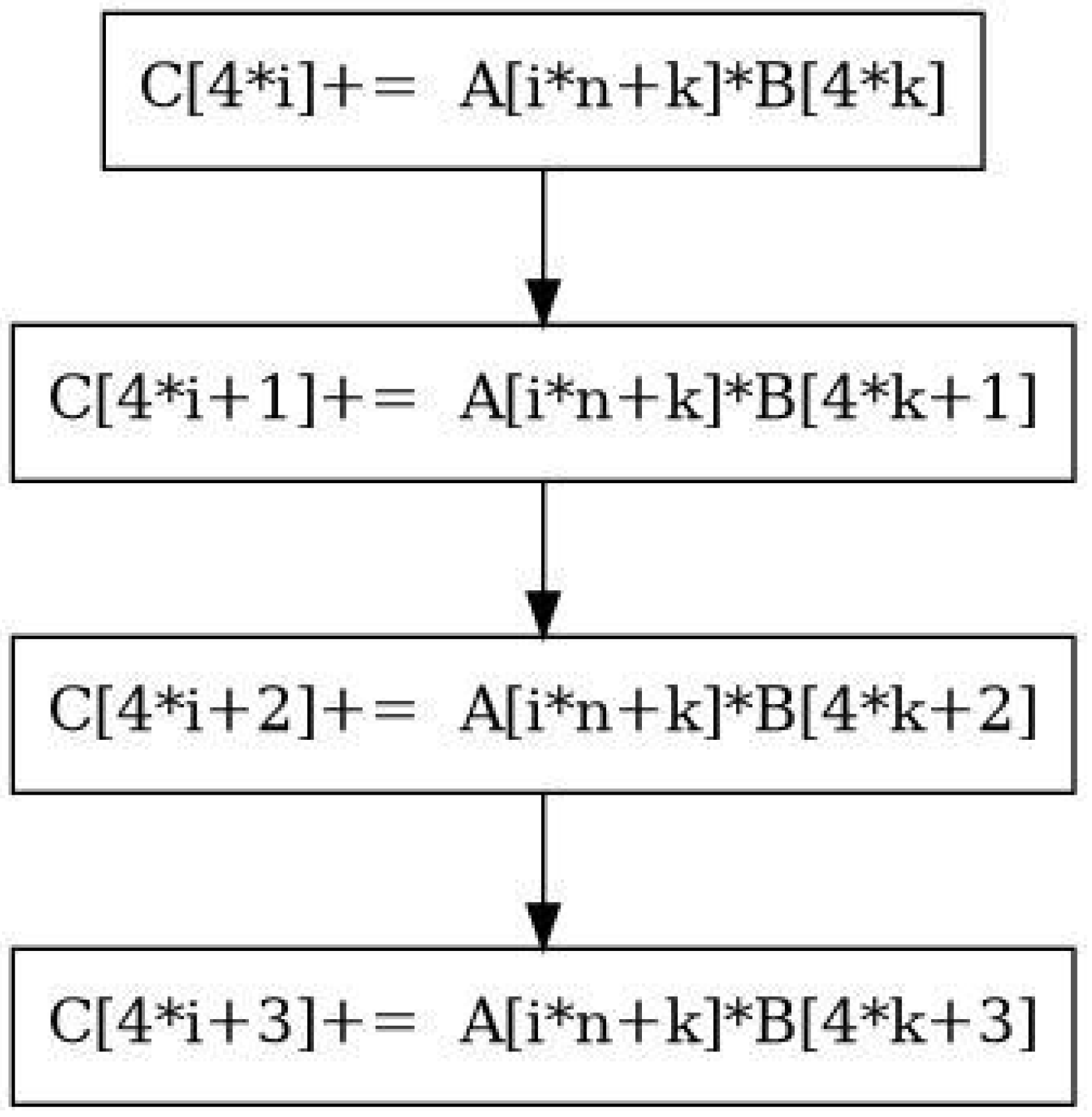
•     { seq (j=0;j<4;j++)
•        { C[(4∗i)+j]+=A[(i∗n)+k]∗B[(4∗k)+j]; }
•     }

The execution graph is then a linear chain of such blocks (Figure 4). (The inner loop is proportional to the size of the original MoA expression, so it is reasonable and customary to treat it as an atomic block of sequential instructions).

If on the contrary the compiler choice was parallel execution, the explicit is

• Example 4. 
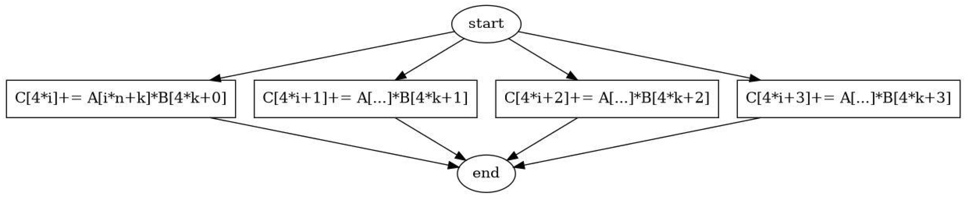
•     { par (j=0;j<4;j++)
•        { C[(4∗i)+j]+=A[(i∗n)+k]∗B[(4∗k)+j]; } }

And the execution graph would be the one shown in (Figure 5).

In complexity theory, these two variants are considered equivalent for work, i.e., arithmetic operation count, but of course parallel time is $O\left(1\right)$ for the parallel variant, while it is $O\left(p\right)$ in the sequential variant, assuming $p=4$ processing units. But concrete parallel algorithms are either designed by humans at static time, by compilers at compile time or by the runtime. They are never fully parallel but rather block-parallel. A block-parallel version of our example comes by splitting the loop into two blocks of two sequential lines each.

• Example 5. 
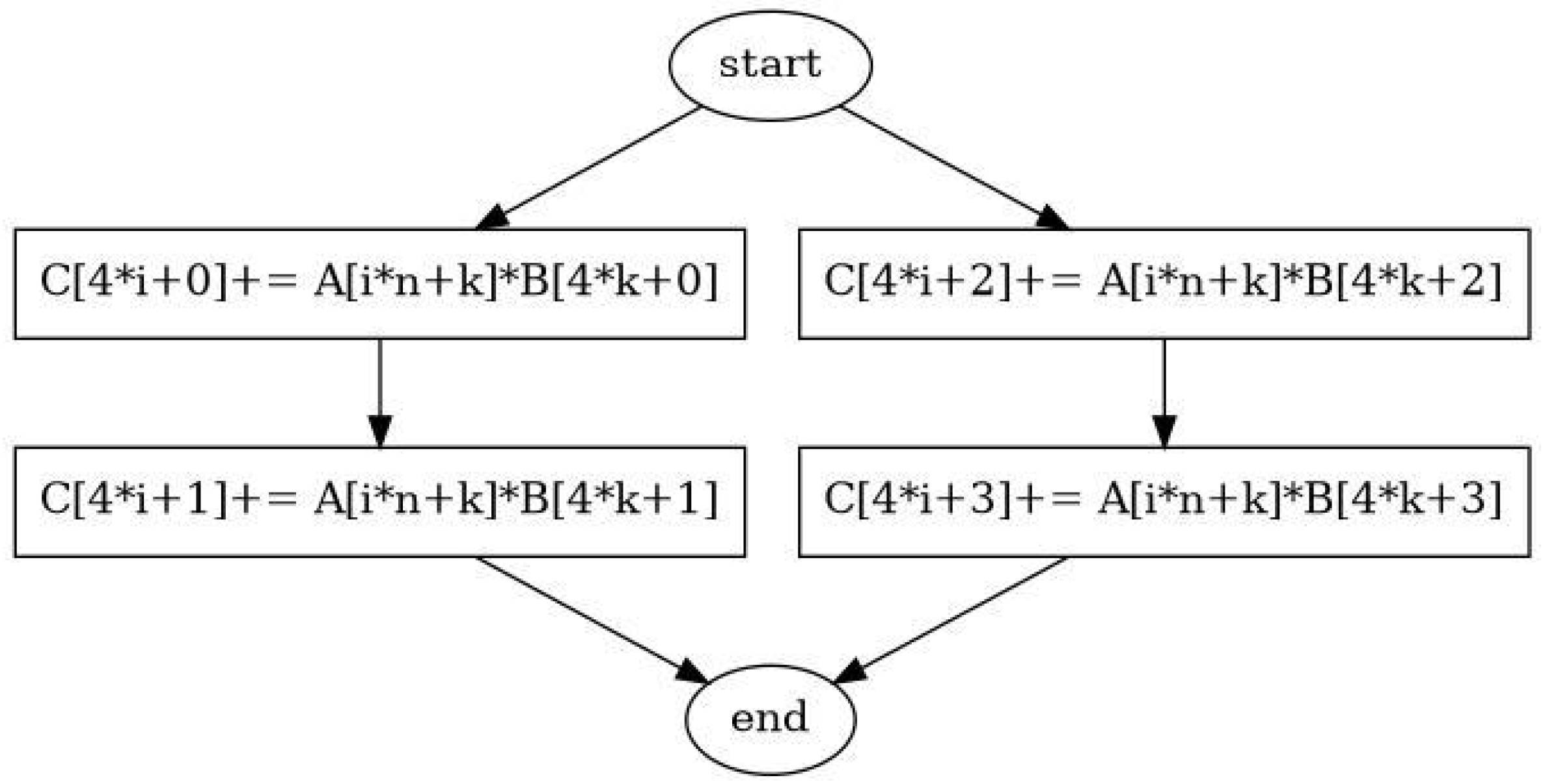
• { par (proc=0;j<2;j++)
•   { seq (jseq=0;jseq<2;j++)
•    { C[(4∗i)+(2∗proc)+jseq]+=A[(i∗n)+k]∗B[(4∗k)+(2∗proc)+jseq]; }  }}

The execution graph becomes (Figure 6).

This type of block decomposition can happen in a variety of combinations, depending on block sizes, which loop is being split, whether the seq-par alternation is nested, etc. In [14], we have exhaustively explored this combinatorial space in Example 2 and target architectures with the two lowest levels of parallelism, namely, vector registers and multiple cores. An analysis of the timings reveals that optimal choices are made when algorithm block sizes are exactly or close to the architecture’s vector register size and/or number of cores. This behavior is known to apply to all levels of parallel architectures: multiple nodes, GPU/TPU processing units, etc. As a result, a mathematical theory can be built that relates algorithm shape with estimated processing time. That theory has two parts:

1.

Producing explicit seq–par loops from MoA expressions. This is called dimension lifting because it increases the number of dimensions in one of the arrays [14], and corresponds to the transformation from a par to a par–seq loop, as seen above. Dimension lifting is a purely algebraic transformation applied to the DNF, using the reshape $\rho$ operator, and its effect on the ONF or fragment-C code is to produce blocks that are executed in parallel. The space of possible dimension liftings is essentially that of possible reshaping operations on the given algorithm. The laws of linear algebra ensure that all such transformations preserve the algorithm’s result.

2.

Estimating the cost, i.e., estimated execution time of each algorithm variant. This builds on algorithmic theories like BSP [10] and its hierarchical variant, the scatter–gather language SGL [15]: the cost of an execution graph combines instruction counts and transfer (effects of bandwith, or synchronization, i.e., latency) times. In practice, the cost can be either normalized in units of arithmetic operations (assuming that their rate per second is mostly stable) or purely in (fractions of) seconds. The appropriate theory for defining costs comes from operations research, namely, weights from a semi-ring that label the edges/nodes of a directed graph [39].

• Semi-rings are the two-operation algebras (abstract addition, abstract multiplication) that may not have inverses: generalized rings where subtraction and division are not generally defined (e.g., max+ algebras, where the abstract addition is maximum and the abstract multiplication is the addition of costs). Gondran & Minoux [39] among others have shown how the max+ algebra is the correct mathematics to compute longest paths in graphs, once edges are given costs from that algebra. The abstract definitions are useful to show many other costs than max+ (i.e., maximal execution time over possible computation paths).

Counting arithmetic operations poses no conceptual problem. The basic step in our algorithm is of the form C[(i∗p)+j]+= A[(i∗n)+k]∗B[(k∗p)+j], so it requires 4 multiplications (3 to evaluate the right-hand side expression and 1 to evalue the left-hand-side index) and 4 additions (3 for indices and 1 for accumulation +=). Let us assume that this amounts to 8 units of time.

The semi-ring is $(\mathbf{N},max,+,0,0)$, so we associate a unit of time to every edge or node being traversed, accumulate them by addition on any path and compute the maximal cost for a path in the algorithm-directed acyclic graph (dag). But applying this theory to pure arithmetic costs would not satisfy the physical requirement for transfer times.

The mathematical requirement is trivial: to associate costs not only to the nodes being traversed, but also to the edges. The scientific problem however is extremely difficult: to associate such costs in a manner that it models actual measurements on computer architectures. This problem is compounded by the great variety and non-scientific design culture of processors and computers. But the decades of experiments with multinode systems, the BSP cost model [12], and our recent experiments with GPU [40] and vector-multicore CPU systems [14] confirm all of the above remarks: linear-algebraic combinations of transfer and arithmetic costs, structured in hierarchical blocks that match the hardware structures, define a tractable and realistic search space for optimal and predictable performance.

Assume that the target architecture has two processing units. We have seen that every basic execution block requires 8 arithmetic time units. It also requires one read (load) from array B, one write (store) to array C, and at most one read (load) from array A. Assume that the cost of an arithmetic operation is one unit of time, and that of a transfer operation is $t:\mathbf{N}$. Realistic values of t can range from a dozen to thousands, depending on the specific hardware level. Then, it proceeds as follows:

• [seq] When executing the seq algorithm variant, only one processing unit is active and it may “prefetch” the A element A[(i∗n)+k], i.e., load it only once because it is independent of loop index j. Each one of the four sequential steps requires a read from B and write to C. Thus, the overall arithmetic cost is that of read(A), followed by four time (read(B);write(C)), i.e., $9t$. The arithmetic cost is the sum of the cost of one step $4\times 8$.
• [par] When executing the par algorithm variant, we exceed the capacity for parallel execution by creating four parallel processes or threads. As a result, the two processing units will interleave the four steps. The degree of parallelism implies that the arithmetic cost is the sum of the costs of two sequential steps. In other words, the arithmetic cost of one thread is $2\times 8$. For transfer costs, our model is as follows: each thread may load(A) a single time, but there is no guarantee that the hardware can process this concurrent read in one step. Our modeling is such that it could cost $2t$ if that operation is serialized. Each thread reads from B twice, and that is fully independent between the threads because the array elements are distinct. Each thread also writes to C twice, also a fully parallel operation. As a result, the transfer cost is $2t+2t+2t=6t$.
• [parseq] When executing the parseq algorithm, the loops create exactly two threads of two sequential steps each, which matches hardware size. The arithmetic cost is the same as the (two-thread) execution of par: $2\times 8$. However, each thread is able to amortize the loading of A[(i∗n)+k] because the sequence of two operations is known at compile time, and not the effect of dynamic thread scheduling. Accordingly, each processing unit reads from A only once, then reads twice from B and writes twice to C. The transfer cost is then $5t$. The costs are summarized in

  Table 1. Costs of algorithm variants.

  Algorithm Variant	Arithmetic	Transfer	Cost
  seq(4)	$4\times 8$	$9t$	$9t+32$
  par(4)	$2\times 8$	$6t$	$6t+16$
  parseq(2,2)	$2\times 8$	$5t$	$5t+16$

  .

Two conclusions can be drawn from our thought experiment. They are specific to this example but, because of the physical properties of hardware, they are experimentally verified:

1.

Sequential execution is slowest. This holds when $t>1$, and this is true except in very unusual contexts.

2.

Block-conscious parallel algorithm variant is fastest because it maximizes the use of static information about data and architecture shapes. In our tiny example, this led to the economy of one load operation while retaining gain.

MoA dimension lifting can thus explore block-parallel variants of a given algorithm with the assurance of finding a cost that is optimal for the standard arithmetic+transfer measurements. There is a huge side-effect of this methodology that is not explicit here: some parallel compilation methods attempt to match a random computation graph to a random architecture structure, which leads to an intractable problem similar to job scheduling. By contrast, the MoA-based exploration of algorithm variants by reshaping leads to a tractable and usually optimal cost.

6.4. General Costs

We can now generalize from the above observations and summarize our applied mathematical basis for MoA-based parallel computing.

A given mathematical expression on arrays, expressed with MoA, can be transformed to DNF, which is equivalent to an ONF and in-turn a fragment-C loop-nest program. That program’s computation dag is highly symmetric and need not be enumerated: its loop sizes (array shapes) are sufficient to describe it.

Many equivalent variants of the computation dag can be produced by dimension-lifting. This search space can be restricted to block sizes that match the architecture: size of the vector registers, number of cores, number of supercomputer nodes, etc. But it can cover the combinatorial space of dimensions: each subset of the array dimensions can be “dimension lifted”, i.e., split into blocks. For example, a two-dimensional array can have its rows divided, or its columns, or both. The first two options produce a 3-dimensional array and the last one produces a 4-dimensional array.

For each computation dag derived in this manner, a cost estimate can be produced by applying some experimental estimate and architecture knowledge: parallel or sequential execution, load-store protocols and delays, communication or synchronization delays, etc. Once the costs for each step and transfer are produced, they can be combined with the semi-ring operations: max for parallel parts of the graph, and + for successive parts.

Here are arguments for using the general theory of semi-rings in this context, the max+ algebra being the most typical example, but not general enough:

• The $\mathbf{N}$ values are obviously too simplistic. If costs are measured in seconds, then fractions will appear so the base type can be that of rationals.
• If the architecture is hierarchical, then so should the computation dags be. In that case, the semi-ring elements could be vectors of costs, combined with pointwise addition and vector-to-rational maximum.
• For abstract reasoning, it may be possible to define the graphs from regular expressions, in which case the semi-ring elements become languages (sets) of abstract costs, + is replaced by concatenation, and max is replaced by union.
• In modern processors, it often happens that the clock rate changes over time, so the constant arithmetic rate hypothesis becomes unrealistic. Cost then become time series; + can be replaced by concatenation and max by the maximum of some integral or statistics on the time series.

For all the above reasons, we introduce the following definition for parallel execution costs. It is fully axiomatic and we have provided arguments that it leads to a fruitful interaction between algebra and performance evaluation/optimization.

Definition 24. 

A parallel execution cost structure is a: $(\mathcal{G},(\mathcal{C},\oplus ,\odot ,Ø,\mathcal{Z})$, cost, α)

1.

An infinite family $\mathcal{G}$ of finite directed acyclic graphs $g\in \mathcal{G}$ whose nodes x are called instructions and whose edges $(x,y)$ are called (data) transfers, such that every $g\in \mathcal{G}$ has a single source and single sink.

2.

An (additively) idempotent semi-ring $(C,\oplus ,\odot ,Ø,Z)$ with total order < for which both operations are increasing: $x\le (x\oplus y)$, $x\le x\odot y$ and $y\le x\odot y$.

3.

A cost function that associates an element of C to every node and edge of any graph $g\in \mathcal{G}$.

4.

An $\{\oplus ,\odot \}$-coloring α of the nodes of every graph g (except the sink) such that, if $\alpha \left(x\right)=\odot$, then x is called a sequential node and has exactly one outgoing edge, or, if $\alpha \left(y\right)=\oplus$, then y is called a parallel node and has more than one outgoing edge.

The example execution graphs above illustrate trivial cases of the family of graphs, the two-coloring and the costs. General execution cost is defined on sequential-parallel graphs of any nesting depth and size, and the following general definition of graph cost.

Definition 25. 

Given a parallel execution cost structure $(\mathcal{G},(\mathcal{C},\oplus ,\odot ,Ø,\mathcal{Z})$, cost, α), the cost C of a dag $g\in \mathcal{G}$ is defined recursively by its source node:

• If z is the graph sink, then $C\left(z\right)=Z$.
• If $(x,x^{\prime })$ is the unique outgoing edge from a sequential node x, then $C\left(x\right)=\mathtt{cost}\left(x\right)\odot C\left(x^{\prime }\right)$.
• If $(y,y_1),(y,y_2)\dots (y,y_k)$ are the outgoing edges from a parallel node y, then $C\left(y\right)=\mathtt{cost}\left(y\right)\odot (C\left(y_1\right)\oplus \dots C\left(y_k\right))$.

The definition of graph cost we have used in our examples uses the max-+ semi-ring $(\mathbf{N},max,+,0,0)$, once the execution and transfer costs are evaluated as natural numbers. It is also possible to use a semi-ring of time-dependent natural numbers (to model variable clock rate in the architecture), a semi-ring of rational numbers (to model actual delays in seconds and not in instructions counts) or any complex combinations that the axioms allow.

Finally, we give an abstract form of the effect of MoA dimension-lifting on computation costs that may inspire more general applications and theorems.

Definition 26. 

A dimension lifting on a cost structure is an internal map $L:\mathcal{G}\to \mathcal{G}$, such that (a) L(g) is a node permutation of g; (b) preserves the cost of nodes and edges: cost(x) = cost(L(x)), cost(x, x′) = cost(L(x), L(x′)) and (c) reduces the length of every sequential chain.

Theorem 2. 

If L is a dimension-lifting on G and C and $g\in \mathcal{G}$, then $C\left(L\right(g\left)\right)\le C\left(g\right)$.

Proof. 

By the recursive definition of (sub)graph cost, the complete graph’s cost $C\left(x\right)$ is an expression on operators $\oplus ,\odot$. By the definition of L, $L\left(x\right)$ contains the same semi-ring values but every sequential chain of nodes is shorter. From the properties $x\le x\odot y$ and $x\le x\odot y$, it follows that the cost of every sequential chain starting at a node $x_0$ is less in (the graph rooted at) $L\left(x_0\right)$ than in (the graph rooted at) $x_0$. Given a parallel node $y_0$, its local cost $\mathtt{cost}\left(y_0\right)$ is preserved, by the definition of L. Moreover, by induction, on the depth of the subgraph, the cost of its subgraphs $y_1,\dots ,y_k$ are also decreased through L. As a result,

• $C\left(L\left(y_0\right)\right)=$
• $\mathtt{cost}\left(L\left(y_0\right)\right)\odot (C\left(L\left(y_1\right)\right)\oplus \dots \oplus C\left(L\left(y_k\right)\right))=$
• $\mathtt{cost}\left(y_0\right)\odot (C\left(L\left(y_1\right)\right)\oplus \dots \oplus C\left(L\left(y_k\right)\right))\le$
• $\mathtt{cost}\left(y_0\right)\odot (C\left(y_1\right)\oplus \dots \oplus C\left(y_k\right)).$
• □

7. Discussion

7.1. Transpose and Reshape

Another example of the abstract dimension lifting uses so-called binary transpose. Binary transpose permutes chosen dimensions and their indices. It is defined by a permutation of the dimensions, for example, [0, 2, 1, 3] if the array has four dimensions. In Example 1, we explained how it can combine with the reduce operator to allow the reduction of an any dimension in the array, while pure reduction only reduces the first dimension.

It can also combine with the reshape operator to drive the algorithm mapping to processors. In other words, reshaping and permutations define the MoA expression’s ONF so indirectly, the loop bounds of the equivalent fragment-C, and finally the shape of an execution graph for this pseudo-code.

7.2. Mapping Loops to Processing Elements

In Section 6, we gave examples of mapping a single loop to processors, and the block structures in those execution graphs can be created by simple transpose–reshape operations. Those examples were 1-dimensional, but suppose we would want to map blocks that are two-dimensional. Assuming an array $\xi$ of shape $<4,4>$ mapped to two processors, we could reshape it to $<2,2,2,2>$, i.e., the shape of a square 2 × 2 array of 2 × 2 blocks. This type of blocking is ideal for algorithms like the Kronecker Product. By permuting dimensions, i.e., $<0,2,1,3>$, the transpose of a $<2,2,2,2>$-reshaped ${\xi }^{\prime }$, we also permute the indices, thus creating blocks. Thus, for any index $0\le \overrightarrow{i}<\left(\rho {\xi }^{\prime }\right)$ in the reshaped array, each component would be accessed by $<0,2,1,3>\psi {\xi }^{\prime }$.

Why is this blocking useful? Blocking identifies a size relevant to the speed of the closest processor memory, e.g., cache. The blocking size would be related to the cache (or whatever the closest memory unit is) and of course to the elements’ data type and size. As levels of memory emerge in the formulation of costs for arbitrary machines, the blocking would continue recursively as the properties of linear algebra allow, as seen for the example in Strassen matrix multiplication.

7.3. Parallel Architecture as an Array

The above example of cost modeling is as simple as it can be: one loop being parallelized or transformed to a parallel set of smaller loops on blocks of the initial date. In [14], we have applied this concept to many variants of matrix multiplication: column-parallel, row-parallel, and block-parallel, and compared their execution times for all possible combinations of input sizes and compiler directives and for two target architectures.

One may ask how our estimates of execution time can adapt to different target architectures: CPU, GPU, TPU, FPGA, etc. The answer is that we model the target architecture as a symmetric tree whose leaves are processing elements. Because the tree’s shape is symmetric, it is equivalent to an array of processing elements. For example, we can approximate the Fujitsu A64FX as a 4 × 12 array of cores, a Huawei Ascend 910 as a 6 × 4 array of daVinci cores, which are themselves 16 × 16 × 16 FP16 processing units, etc. At the level of vector registers, we can also use array reshaping to fit their sizes as yet another dimension in the architecture array. If the target is a distributed architecture, then we would add an upper dimension. For example, an array of 8 NVIDIA A100 GPUs would be represented as an 8 × 132 array if each GPU has 132 SM units.

Even at this rough level of description, the target architecture provides a better performance when the chunks of operations and data with which it is provided come in sizes that match some of its dimensions. This is the concept that pushes us to explore shape and algebraic transformations based on array shapes.

Finally, we list some fundamental limitations to our cost modeling:

1.

The assumption that the target architecture is a symmetric tree of compute elements and sub-elements is equivalent to requiring that it is homogeneous. In the above example of a cluster of eight, 132 SM-GPUs, our theory does not cover the case of a computation that would also run on the CPUs of the eight nodes. It does apply to a cluster of CPUs of course, but not to a mixture of CPUs and GPUs at the same level of the architecture tree.

2.

For an instance such as the above Example 3, when compiled to different architectures, a given source code will have different branch prediction behavior. Our cost theory does not cover such variations because the target machine instructions are not described in it. This raises two open questions for future work: (a) Can our experiments suggest a simple mathematical description of the effect of branch prediction on performance? (b) If not, can our theoretical cost prediction be improved to produce variation statistics coherent with experiments?

3.

Processor frequency variations are also not covered by our theory for the following reason: our execution time estimates are based on a notion of instruction counts, similar but more concrete than complexity theory. Transforming the instruction count to an execution delay in seconds is not stable if the instruction rate per second is variable. Energy prediction may also vary in the presence of clock frequency variations.

8. Conclusions and Future Work

We have shown how the MoA array algebra is a general and suitable basis for a mathematical theory of parallel computing. From the algebra of algorithms to execution costs, a methodology has been defined and its mathematical basics defined.

Parallel compilation should become an experimental science, and we propose a basis for that evolution. There are enormous implications for that branch of applied mathematics, applying a blend of algebra, operations research, and physics of computation including group theory.

Future research directions include (a) more experimental validation of the cost prediction on varied source codes and target architectures; our array transformations must cover all known high-level optimizations and original ones such as binary vectors to encode sparseness [41], which can be expressed algebraically; (b) non-arithmetic preserving transform in MoA (Winograd- or Strassen-like optimizations that reduce the arithmetic operation count) to generalize the dimension-lifting transforms; (c) the mechanization of MoA and of MoA-based compilation; (d) mathematical goal—the application of Vitanyi’s [42] results, which can relate the orbits of symmetry groups on MoA expressions to lower bounds on lengths in space-time.

References

- Jenkins, M.A.; Mullin, L.R. A Comparison of Array Theory and a Mathematics of Arrays. In Arrays, Functional Languages, and Parallel Systems; Mullin, L.M.R., Jenkins, M., Hains, G., Bernecky, R., Gao, G., Eds.; Springer: Boston, MA, USA, 1991; pp. 237–267. [Google Scholar] [CrossRef]
- Markus, A.; Mullin, L. Array Access and Performance Regarding Numerical Algorithms. Trans. Eng. Comput. Sci. 2026, 14, 1–14. [Google Scholar] [CrossRef]
- Kennedy, K.; Koelbel, C.; Zima, H. The rise and fall of High Performance Fortran: An historical object lesson. In Proceedings of the Third ACM SIGPLAN Conference on History of Programming Languages; Association for Computing Machinery: New York, NY, USA, 2007; pp. 7-1–7-22. [Google Scholar]
- Ritchie, D.M.; Johnson, S.C.; Lesk, M.E.; Kernighan, B.W. The C programming language. Bell Sys. Technol. J. 1978, 57, 1991–2019. [Google Scholar] [CrossRef]
- Clarke, L.; Glendinning, I.; Hempel, R. The MPI message passing interface standard. In Proceedings of the Programming Environments for Massively Parallel Distributed Systems: Working Conference of the IFIP WG 10.3, 25–29 April 1994; Springer: Berlin/Heidelberg, Germany, 1994; pp. 213–218. [Google Scholar]
- Dagum, L.; Menon, R. OpenMP: An industry standard API for shared-memory programming. IEEE Comput. Sci. Eng. 1998, 5, 46–55. [Google Scholar] [CrossRef]
- Farber, R. CUDA Application Design and Development; Elsevier: Amsterdam, The Netherlands, 2011. [Google Scholar]
- Farber, R. Parallel Programming with OpenACC; Newnes: Oxford, UK, 2016. [Google Scholar]
- Pytorch Foundation. Pytorch Documentation. Available online: https://docs.pytorch.org/docs/stable/index.html (accessed on 1 April 2026).
- Valiant, L.G. Why BSP computers? (bulk-synchronous parallel computers). In Proceedings of the [1993] Proceedings Seventh International Parallel Processing Symposium; IEEE: New York, NY, USA, 1993; pp. 2–5. [Google Scholar]
- McColl, W.F. Scalability, portability and predictability: The BSP approach to parallel programming. Future Gener. Comput. Syst. 1996, 12, 265–272. [Google Scholar] [CrossRef]
- McColl, W.F.; Tiskin, A. Memory-efficient matrix multiplication in the BSP model. Algorithmica 1999, 24, 287–297. [Google Scholar] [CrossRef]
- Williams, S.; Waterman, A.; Patterson, D. Roofline: An insightful visual performance model for multicore architectures. Commun. ACM 2009, 52, 65–76. [Google Scholar] [CrossRef]
- Mullin, L.; Hains, G. Towards Automatic, Predictable and High-Performance Parallel Code Generation. In Proceedings of the Parallel and Distributed Processing Techniques (CSCE/PDPTA2024); Arabnia, H.R., Takata, M., Deligiannidis, L., Rivas, P., Ohue, M., Yasuo, N., Eds.; Springer: Cham, Switzerland, 2025; pp. 109–119. [Google Scholar]
- Li, C.; Hains, G. SGL: Towards a bridging model for heterogeneous hierarchical platforms. Int. J. High Perform. Comput. Netw. 2012, 7, 139–151. [Google Scholar] [CrossRef]
- Gerbessiotis, A.V. Extending the BSP model for multi-core and out-of-core computing: MBSP. Parallel Comput. 2015, 41, 90–102. [Google Scholar] [CrossRef]
- Allombert, V.; Gava, F.; Tesson, J. Multi-ML: Programming multi-BSP algorithms in ML. Int. J. Parallel Program. 2017, 45, 340–361. [Google Scholar] [CrossRef]
- Legaux, J.; Hu, Z.; Loulergue, F.; Matsuzaki, K.; Tesson, J. Programming with BSP homomorphisms. In Proceedings of the European Conference on Parallel Processing; Springer: Berlin/Heidelberg, Germany, 2013; pp. 446–457. [Google Scholar]
- Ofenbeck, G.; Steinmann, R.; Caparros, V.; Spampinato, D.G.; Püschel, M. Applying the roofline model. In Proceedings of the 2014 IEEE International Symposium on Performance Analysis of Systems and Software (ISPASS); IEEE: New York, NY, USA, 2014; pp. 76–85. [Google Scholar] [CrossRef]
- Treibig, J.; Hager, G. Introducing a performance model for bandwidth-limited loop kernels. In Proceedings of the International Conference on Parallel Processing and Applied Mathematics; Springer: Berlin/Heidelberg, Germany, 2009; pp. 615–624. [Google Scholar]
- Rajopadhye, S.V. Dependence analysis and parallelizing transformations. In The Compiler Design Handbook; Srikant, Y.N., Shankar, P., Eds.; CRC Press: Boca Raton, FL, USA, 2003. [Google Scholar]
- Berkling, K. Arrays and the Lambda Calculus; Technical Report; Syracuse University: Syracuse, NY, USA, 1990. [Google Scholar]
- Hains, G.; Mullin, L.M.R. Parallel functional programming with arrays. Comput. J. 1993, 36, 238–245. [Google Scholar] [CrossRef]
- Hunt, H.; Mullin, L.; Rosenkrantz, D.; Raynolds, J. A Transformation–Based Approach for the Design of Parallel/Distributed Scientific Software: The FFT. arXiv 2008, arXiv:0811.2535. [Google Scholar] [CrossRef]
- Mullin, L.R.; Raynolds, J.E. Conformal Computing: Algebraically connecting the hardware/software boundary using a uniform approach to high-performance computation for software and hardware applications. arXiv 2008, arXiv:0803.2386. [Google Scholar] [CrossRef]
- Grout, I.; Mullin, L. Realizing Mathematics of Arrays Operations as Custom Architecture Hardware-Software Co-Design Solutions. Information 2022, 13, 528. [Google Scholar] [CrossRef]
- Grout, I.; Mullin, L. Realization of the Kronecker Product in VHDL using Multi-Dimensional Arrays. In Proceedings of the 2019 7th International Electrical Engineering Congress (iEECON); IEEE: New York, NY, USA, 2019. [Google Scholar] [CrossRef]
- Mullin, L.M. A Mathematics of Arrays. Ph.D. Thesis, Syracuse University, Syracuse, NY, USA, 1988. Available online: https://www.researchgate.net/profile/Lenore-Mullin/publication/308893116_A_\Mathematics_of_Arrays/links/57fe4f8408aeaf819a5c29ee/A-Mathematics-of-Arrays.pdf (accessed on 1 January 2026).
- Gondhalekar, A.; Feng, W.C. On the Three P’s of Parallel Programming for Heterogeneous Computing: Performance, Productivity, and Portability. In Proceedings of the 2023 IEEE High Performance Extreme Computing Conference (HPEC); IEEE: New York, NY, USA, 2023; pp. 1–7. [Google Scholar] [CrossRef]
- Petit, Q.; Li, C.; Emad, N.; Dongarra, J. Efficient embedding initialization via dominant eigenvector projections. In Proceedings of the SC’25 Workshops of the International Conference for High Performance Computing, Networking, Storage and Analysis, St. Louis, MO, USA, 16–21 November 2025; pp. 1790–1799. [Google Scholar]
- Chen, J.; Li, K.; Tang, Z.; Bilal, K.; Yu, S.; Weng, C.; Li, K. A parallel random forest algorithm for big data in a spark cloud computing environment. IEEE Trans. Parallel Distrib. Syst. 2016, 28, 919–933. [Google Scholar] [CrossRef]
- Grout, I.; Mullin, L. Hardware Considerations for Tensor Implementation and Analysis Using the Field Programmable Gate Array. Electronics 2018, 7, 320. [Google Scholar] [CrossRef]
- Thomas, S.; Mullin, L.; Swirydowicz, K.; Khan, R. Threaded Multi-Core GEMM with MoA and Cache-Blocking. In Proceedings of the 2021 World Congress in Computer Science, Computer Engineering, & Applied Computing (CSCE’21), Las Vegas, NV, USA, 26–29 July 2021. [Google Scholar]
- Mullin, L.R. A uniform way of reasoning about array-based computation in radar: Algebraically connecting the hardware/software boundary. Digit. Signal Process. 2005, 15, 466–520. [Google Scholar] [CrossRef]
- Ostrouchov, C.; Mullin, L. PythonMoA (GitHub Repository). 2022. Available online: https://github.com/Quansight-Labs/python-moa (accessed on 1 April 2026).
- Thomas, S.; Mullin, L.; Świrydowicz, K. Improving the Performance of DGEMM with MoA and Cache Blocking. In Proceedings of the ACM Arrays’21, 20–26 June 2021; National Renewable Energy Laboratory: Golden, CO, USA, 2021. [Google Scholar]
- Hains, G.; Mullins, J.; Mullin, L. Language Foundations for HPC Array Structures. In Proceedings of the 21st International Conference on Foundations of Computer Science (CSCE/FCS’25); Springer: Cham, Switzerland, 2025. [Google Scholar]
- Hager, G.; Treibig, J.; Habich, J.; Wellein, G. Exploring performance and power properties of modern multi-core chips via simple machine models. Concurr. Comput. Pract. Exp. 2016, 28, 189–210. [Google Scholar] [CrossRef]
- Gondran, M.; Minoux, M. Graphs, Dioids and Semirings: New Models and Algorithms; Springer: Berlin/Heidelberg, Germany, 2008. [Google Scholar]
- Mullin, L.; Phan, W. A Transformational Approach to Scientific Software: The Mathematics of Arrays (MoA) FFT with OpenACC. In Proceedings of the OpenACC Annual Summit, Digital Event, 14 September 2021; Available online: https://www.openacc.org/events/openacc-summit-2021 (accessed on 1 April 2026).
- Staccone, S.; Filippone, S.; Sciarria, L.P. Efficient Binary SpMV on GPUs via Binary Word Compression. In Proceedings of the 34th Euromicro International Conference on Parallel, Distributed, and Network-Based Processing (PDP2026), Cluj-Napoca, Romania, 25–27 March 2026. [Google Scholar]
- Vitányi, P.M. Locality, communication, and interconnect length in multicomputers. SIAM J. Comput. 1988, 17, 659–672. [Google Scholar] [CrossRef]