Heterogeneous Transfer Learning for Linear Regression Model with Heteroscedasticity

Abstract

We consider the transfer learning problem in the linear regression model, where the source domain and target domain have different features and the model exhibits heteroscedasticity. The existing homogeneous transfer learning methods cannot yet handle this type of problem. In this work, a transfer learning algorithm is proposed, which integrates data of varying dimensions and accounts for heteroscedasticity, thereby yielding a data-pooling estimator. The algorithm is simple to implement and easy to operate. The theoretical properties of the proposed estimator are established, including an upper bound on the generalization error and robustness against negative transfer. Simulation studies indicate that the proposed method performs well in terms of parameter estimation. The effectiveness of the proposed method is also validated using real-life datasets in UCI public repository, demonstrating favorable performance compared to the existing methods.

1. Introduction

Transfer learning is an important research technique in machine learning and also a new learning paradigm. It focuses on using existing knowledge (namely, source domain) to solve different but related tasks (namely, target domain), addressing the problem of having only a small amount of labeled sample data. It also overcomes the tediousness and inefficiency of learning each task from scratch and building different learning models for each problem. In many practical situations, collecting a large amount of labeled data for each target domain is very expensive and difficult. Therefore, it is necessary for transferring knowledge from related tasks to improve problems in the target domain. Moreover, transfer learning has achieved significant results in fields such as natural language processing, computer vision, and healthcare. As evidenced by these successes, transfer learning represents a powerful and meaningful strategy for improving data efficiency and model performance across diverse applications [1].

Recently, several authors have explored the problem of transfer learning in many statistical models. Tian and Feng [2] discussed the transfer learning under high-dimensional generalized linear models; they proposed a transfer learning algorithm in generalized linear models and achieved a theoretical analysis. In the logistic regression framework, Hou and Song [3] developed a two-step transfer learning algorithm and a non-algorithmic transferable source detection method to offer consistent and robust privacy protection. Transfer learning for nonparametric regression is considered in [4], which studies the non-asymptotic minimax risk of transfer learning in nonparametric regression and develop a confidence thresholding estimator that achieves the minimax optimal risk up to a logarithmic factor. Lin and Reimherr [5] studied the transfer learning for the functional linear regression under the reproducing kernel Hilbert space framework. Jin et al. [6] extended transfer learning methodology to quantile regression settings, developing a framework for detecting informative sources and enhancing estimation accuracy in applications such as flight safety analysis. He et al. [7] developed a semiparametric transfer learning framework that leverages shared representations while modeling domain-specific heterogeneity. Transfer learning has also been applied in other models, such as in [8,9,10].

While some of the aforementioned methods offer statistical frameworks in various statistical models, they are limited by a crucial assumption. It is assumed that the target and source populations have identical covariates or features at their disposal, which is also known as homogeneous transfer learning. Nevertheless, this assumption is impractical in many real-world applications. For example, in biomedical studies, the target domain on a specific patient population has a limited amount of data, and only a few key variable features can be collected, while the source data or related electronic health record can be easily obtained, and more features can be measured, which is referred to as heterogeneous transfer learning. At this point, homogeneous transfer learning limits their practical applicability. The challenge of learning from source datasets with diverse feature spaces has been investigated in research, such as [11,12]. Peng and Wang [13] assumed that auxiliary samples were collected from different sub-populations with non-negligible heterogeneity and developed a strategy to leverage possible shared information from relevant source datasets. Karbalayghareh et al. [14] proposed a novel Bayesian method to allow a robust partial information transfer by imposing a spike-and-slab prior on the joint distribution of parameters in the proxy and target domain. Chang et al. [15] introduced a heterogeneous transfer learning for high dimensional regression with different features. Silvestrin et al. [16] developed a transfer learning technique in the linear regression versions with different input dimensions. Recently, considerable progress has been made in heterogeneous transfer learning under high-dimensional settings. Most existing high-dimensional heterogeneous frameworks focus on feature heterogeneity or distribution shift while rarely integrating systematic heteroscedasticity modeling into linear regression transfer inference. In this work, we consider this issue and develop a transfer learning strategy to heteroscedastic linear regression under cross-domain heterogeneity, thereby extending the scope of the existing heterogeneous transfer learning methods to accommodate heteroscedastic error structures.

As is well known, heteroscedasticity is a critical phenomenon that significantly impacts the validity and reliability of regression models. Its presence can lead to inefficient and biased parameter estimates, thereby undermining the accuracy of predictions and inferences. White [17] demonstrates that heteroscedasticity biases standard error estimation and proposes a consistent covariance matrix estimator to restore valid inference. Wooldridge [18] further stresses that, in finite samples and complex data settings, uncorrected heteroscedasticity substantially distorts test statistics and confidence intervals. Berenguer-Rico and Wilms [19] reveal that even preliminary data-cleaning steps, such as outlier removal, can interact with heteroscedasticity to induce size distortion in hypothesis testing. Recognizing and addressing heteroscedasticity is essential for enhancing the robustness of statistical analysis and ensuring that the conclusions drawn from data are sound and trustworthy. Based on the above analysis, it is of great significance to conduct research on heterogeneous transfer learning in linear regression with heteroscedasticity. Informed by prior research, a novel estimator termed heteroscedastic data-pooling (HDP) is developed herein for linear regression with heteroscedasticity, which effectively integrates datasets from source and target domains that contain different features. To address this issue, an efficient and easily implementable heterogeneous transfer learning algorithm is developed, for which an upper bound on the generalization error is established through a theoretical analysis. The robustness of the estimator is confirmed by numerous simulation experiments and real data analysis.

Although the existing heterogeneous regression-based transfer methods (e.g., [13,15,16]) have made progress in handling feature heterogeneity across domains, they generally fail to explicitly model domain-specific heteroscedastic noise or construct dedicated estimators that can adapt to both heterogeneous feature spaces and heteroscedasticity. Different from these prior approaches, the HDP estimator proposed in this paper explicitly characterizes the heteroscedastic structure in both source and target data, and achieves effective integration of cross-domain data with different features, which distinguishes our method from existing heterogeneous regression-based transfer approaches.

The main contributions and innovations of this paper can be summarized as follows:

• We address the problem of transfer learning when the source and target domains have inconsistent feature dimensions and heteroscedastic noise, which is rarely considered in existing studies.
• We propose a novel Heteroscedastic Data-fusion Predictor (HDP), which constructs a robust transfer learning objective by weighted fusion of source and target domain data.
• We derive the estimation error upper bound for the proposed HDP estimator, providing theoretical guarantees for its performance under heteroscedasticity and feature misalignment.
• Extensive simulations and experiments demonstrate that HDP effectively leverages source domain information while maintaining robustness against feature mismatch and heteroscedastic noise in the target domain.

The differences between the contributions of this paper and those of existing works are summarized as follows. Chang et al. [15] considers a homoscedastic linear regression model and assumes that some features present in the source data are missing in the target domain. In contrast, our work accounts for heteroscedasticity in the model and assumes that some features in the target data are missing in the source domain. Compared with Silvestrin et al. [16], our work explicitly incorporates heteroscedasticity into the modeling framework. Zhao et al. [20] studies heterogeneous transfer learning for high-dimensional generalized linear models. Although it allows the model parameters to differ between the source and target domains, it assumes that the feature spaces of all datasets are identical. By contrast, our work considers the more general setting where the feature spaces of the source and target domains are allowed to be different.

The rest of the paper is organized as follows: Section 2 introduces the model setup and formulates the heterogeneous transfer learning problem under heteroscedastic linear regression. Section 3 presents the heteroscedastic data-pooling estimator. Section 4 provides the theoretical analysis, including the transfer gain and its properties. Section 5 reports both simulation experiments and real-data case studies to evaluate the performance of the proposed method. Finally, Section 6 concludes the paper and discusses future research directions.

2. Model Setup

This article focuses on the problem of learning models based on two datasets: historical data and new data containing additional features. The first one will be referred to as the source dataset, the second as the target dataset. Linear regression is adopted as the modeling framework. The labels in two datasets represent the same linear regression task, but the variance of the error terms in both the source and target domains is heteroscedastic. In this section, we will define the dataset and its distribution in the context of linear regression.

Let the target dataset be defined as $(X_T,{\mathbf{y}}_{\mathbf{T}})$, where $X_T\in {\mathbb{R}}^{n_T\times d_T}$ denotes a full-rank matrix consisting of $n_T$ independent observations with $d_T$ input features, and ${\mathbf{y}}_{\mathbf{T}}\in {\mathbb{R}}^{n_T}$ is a random vector of the corresponding labels. These are associated with the heteroscedastic linear model ${\mathbf{y}}_{\mathbf{T}}=X_T\beta +{\mathbf{w}}_{\mathbf{T}}$, where $\beta$ is a $d_T$-dimensional parameter vector capturing the linear relationship between input features and labels, and ${\mathbf{w}}_{\mathbf{T}}$ is noise that follows a Gaussian distribution $N\left({\mathbf{0}}_{{\mathbf{n}}_{\mathbf{T}}},\mathrm{diag}({\sigma }_1^2,{\sigma }_2^2,\dots ,{\sigma }_{n_T}^2)\right)$, where ${\sigma }_i^2>0$, for $i=1,\dots ,n_T$. The objective of this paper is to learn the parameter vector $\beta$.

Additionally, define the source dataset as $(X_S,{\mathbf{y}}_{\mathbf{S}})$, where $X_S\in {\mathbb{R}}^{n_S\times d_S}$ is a full-rank matrix containing $n_S$ observations with $d_S$ input features ($d_S<d_T$). And ${\mathbf{y}}_{\mathbf{S}}\in {\mathbb{R}}^{n_S}$ stands for the random vector of corresponding labels. The setting $d_S<d_T$ naturally arises from the incremental input transfer learning problem that motivates our work. The opposite case $d_S>d_T$ would essentially become a feature selection or dimensionality reduction problem, which is a different research direction that can be investigated in the future. The relationship between labels and input features in the source dataset is given by ${\mathbf{y}}_{\mathbf{S}}=X_S{\beta }^{\prime }+X^{″}{\beta }^{″}+{\mathbf{w}}_{\mathbf{S}}$, where ${\beta }^{\prime }$ and ${\beta }^{″}$ correspond to the first $d_S$ and last $d_T-d_S$ components of $\beta$, respectively. Here, $X^{″}$ represents a $n_S\times (d_T-d_S)$ random matrix, whose entries $X_{ij}^{″}$ are mutually independent, and each follows a standard normal distribution, i.e., $X_{ij}^{″}\stackrel{\mathrm{i}.\mathrm{i}.\mathrm{d}.}{\sim }N(0,1)$. The assumption that unobserved covariates follow a Gaussian distribution is justified on three grounds. First, it greatly simplifies the theoretical analysis, enabling closed-form derivations of the estimators and their associated properties. Second, although real-world data may not be strictly normal, many features become approximately normally distributed as the sample size increases. Third, the real-data study by Silvestrin et al. [16] demonstrates that, even when the normality condition is not met, the proposed method based on this assumption still yields satisfactory performance. It is further assumed that ${\mathbf{w}}_{\mathbf{S}}$ follows a Gaussian distribution, $N({\mathbf{0}}_{{\mathbf{n}}_{\mathbf{S}}},\mathrm{diag}({\tilde{\sigma }}_1^2,\dots ,{\tilde{\sigma }}_{n_S}^2))$, where ${\tilde{\sigma }}_j^2>0$, for $j=1,\dots ,n_S,$ and is independent of ${\mathbf{w}}_{\mathbf{T}}$. Evidently, the source data follows a heteroscedastic linear model.

Thus, this paper focuses on a linear regression model with a heteroscedastic structure. Furthermore, in the source domain, only a subset of the features available in the target dataset is observable; that is, the newly added features are unknown, while their impact on the labels of both datasets remains consistent (captured by ${\beta }^{\prime }$). The unobserved new features are substituted with random values to account for their influence on the labels. Consequently, the distributions of the source and target domain labels ${\mathbf{y}}_{\mathbf{S}}$ and ${\mathbf{y}}_{\mathbf{T}}$ can be derived as follows:

$${\mathbf{y}}_{\mathbf{S}}\sim N(X_S{\beta }^{\prime },\mathrm{diag}({\tilde{\sigma }}_1^2+\parallel {\beta }^{″}{\parallel }^2,{\tilde{\sigma }}_2^2+\parallel {\beta }^{″}{\parallel }^2,\dots ,{\tilde{\sigma }}_{n_S}^2+\parallel {\beta }^{″}{\parallel }^2\left)\right),$$

(1)

$${\mathbf{y}}_{\mathbf{T}}\sim N(X_T\beta ,\mathrm{diag}({\sigma }_1^2,{\sigma }_2^2,\dots ,{\sigma }_{n_T}^2)),$$

(2)

where $\parallel {\beta }^{″}{\parallel }^2={\sum }_{k=1}^{d_T-d_S}{\left({\beta }_k^{″}\right)}^2$, and ${\beta }_k^{″}$ is the k-th element of the vector ${\beta }^{″}$. All $\parallel ·\parallel$ used in this paper denote the ${\ell }_2$ norm; i.e., for a matrix, $▵\in {\mathbb{R}}^{m\times n}$, the ${\ell }_2$ norm is defined as $\parallel ▵\parallel =\sqrt{{\sum }_{i=1}^m{\sum }_{j=1}^n{\left({▵}_{ij}\right)}^2}.$ Proof details are presented in Appendix A.

In this work, the parameters of the heteroscedastic model are estimated using the generalized least squares method (GLS). For illustration, we focus on the estimation in the target domain. Let ${\mathrm{\Sigma }}_T=diag({\sigma }_1^2,{\sigma }_2^2,\dots ,{\sigma }_{n_T}^2)$. Based on the distributional assumption of ${\mathbf{w}}_T$ above, it follows that ${\mathrm{\Sigma }}_T$ is a positive definite matrix. According to the Cholesky decomposition theorem, there exists a lower triangular matrix, $C_T$, such that ${\mathrm{\Sigma }}_T=C_T{C_T}^T$. Multiplying both sides of the model ${\mathbf{y}}_T=X_T\beta +{\mathbf{w}}_{\mathbf{T}}$ by the matrix $C_T^{-1}$, we obtain the transformed model ${\tilde{\mathbf{y}}}_T={\tilde{X}}_T\beta +{\tilde{\omega }}_T$, where ${\tilde{\mathbf{y}}}_T=C_T^{-1}{\mathbf{y}}_T$, ${\tilde{X}}_T=C_T^{-1}{X}_T$, and ${\tilde{\omega }}_T=C_T^{-1}{\omega }_T$. Since $Var\left({\tilde{\omega }}_T\right)$ = ${C_T}^{-1}{\mathrm{\Sigma }}_T{\left({C_T}^{-1}\right)}^T$, substituting ${\mathrm{\Sigma }}_T=C_T{C_T}^T$ yields $Var\left({\tilde{\omega }}_T\right)={C_T}^{-1}\left(C_T{C_T}^T\right){\left({C_T}^{-1}\right)}^T=I$. This transformation converts the original heteroscedastic models into homoscedastic forms, allowing the application of ordinary least squares (OLS) to the transformed model and yielding a generalized least squares estimator that inherently accounts for heteroscedasticity. The resulting estimator is given by:

$${\widehat{\beta }}_T^{*}={\left({X_T}^T{\left(C_T{C_T}^T\right)}^{-1}{X}_T\right)}^{-1}{X_T}^T{\left(C_T{C_T}^T\right)}^{-1}{\mathbf{y}}_{\mathbf{T}}.$$

(3)

Similarly, for the source domain model, an analogous transformation can be applied. It is evident from the assumption on ${\mathbf{w}}_S$ that ${\mathrm{\Sigma }}_S=diag({\tilde{\sigma }}_1^2,\dots ,{\tilde{\sigma }}_{n_S}^2)$ is positive-definite. Specifically, there exists a matrix $C_S$ satisfying ${\mathrm{\Sigma }}_S=C_S{C}_S^T,$ such that, after multiplying both sides of the source model by $C_S^{-1}$, the transformed model has homoscedastic errors.

At this stage, the source and target datasets, together with their underlying distributions, have been formally specified. Within the heteroscedastic linear regression framework, the GLS estimation procedure for both domains has been introduced. By applying the Cholesky decomposition to the covariance structure of the noise terms, the original heteroscedastic models are transformed into equivalent homoscedastic representations, which enables the direct application of OLS techniques. These results establish the statistical foundation and estimation tools required for the subsequent construction of transfer learning estimators under incremental input settings.

Basic Estimator: To highlight the performance improvement brought by the source dataset, this paper selects a model that uses only the target data as the baseline and chooses the OLS estimator, which is widely used to solve linear regression problems to calculate the loss by minimizing the sum of squared residuals of the target data:

$${\mathcal{R}}_T\left(\beta \right)={∥{\mathbf{y}}_{\mathbf{T}}-X_T\beta ∥}^2.$$

(4)

Therefore, the basic estimator is defined as:

$${\widehat{\beta }}_T={\left(X_T^T{X}_T\right)}^{-1}{X}_T^T{\mathbf{y}}_{\mathbf{T}}.$$

(5)

The OLS is chosen as the baseline because it is the maximum likelihood estimator using $(X_T,{\mathbf{y}}_T)$ and is widely used to solve linear regression problems. Furthermore, ordinary least squares also possesses two favorable statistical properties: unbiasedness and efficiency.

3. Heteroscedastic Data-Pooling Estimator

Building upon the heteroscedastic linear regression model and the estimation framework developed in the previous section, this section proposes a transfer learning approach for incremental input settings. The method leverages information from both the source and target domains while explicitly accounting for heteroscedasticity and discrepancies in the observed feature spaces.

Heteroscedastic data-pooling loss: To integrate information from the source and target domains under heteroscedastic noise, we construct a unified empirical risk that jointly incorporates domain-specific loss functions. The proposed data-pooling loss combines the source and target risks through a weighted scheme, where each component is adjusted according to its corresponding noise covariance structure.

This formulation provides a principled mechanism for balancing the contributions of the two domains while accounting for discrepancies in noise levels and observed feature spaces. A common transfer learning approach is to learn by minimizing the convex sum of errors from two datasets. In the case of linear regression, this method is known as data-pooling. This paper defines the data-pooling loss ${\mathcal{R}}_{\alpha }\left(\beta \right)$ as the weighted sum of the losses from the source and target datasets (denoted as ${\mathcal{R}}_S$ and ${\mathcal{R}}_T$, respectively):

$${\mathcal{R}}_{\alpha }\left(\beta \right)={\alpha }_S{\mathcal{R}}_S\left(\beta \right)+{\alpha }_T{\mathcal{R}}_T\left(\beta \right).$$

(6)

It is clear that, when ${\alpha }_T\gg {\alpha }_S$, the error of the target dataset is magnified compared to the error of the source dataset, and the solution obtained by optimizing ${\mathcal{R}}_T\left(\beta \right)$ will be closer to the baseline estimator. On the other hand, when ${\alpha }_T\ll {\alpha }_S$, ${\mathcal{R}}_S\left(\beta \right)$ will dominate the loss, and the optimal solution will deviate from the baseline estimator.

In the incremental input setting, a key consideration is to isolate the influence of parameters corresponding to newly introduced features on the source-domain error. To this end, this paper defines ${\mathcal{R}}_S\left(\beta \right)={∥{\mathbf{y}}_S-x_S{\mathbb{I}}^{\top }\beta ∥}^2$, where $\mathbb{I}$ represents a $d_T\times d_S$ matrix, such that ${\mathbb{I}}_{ii}=1$ and ${\mathbb{I}}_{ij}=0$ when $i\ne j$. The operation $X_S{\mathbb{I}}^{\top }$ effectively performs dimension expansion on the source-domain feature matrix, where absent dimensions are filled with zero values. Through the algebraic substitution of both ${\mathcal{R}}_S\left(\beta \right)$ and ${\mathcal{R}}_T\left(\beta \right)$ into the unified optimization framework, we derive the following analytical solution. Proof details are presented in Appendix A.

$$\begin{array}{cc}\hfill {\mathcal{R}}_T\left(\beta \right)& ={∥{\mathbf{y}}_{\mathbf{T}}-X_T\beta ∥}^2={∥C_T({\tilde{\mathbf{y}}}_T-{\tilde{X}}_T\beta )∥}^2\hfill \\ \hfill {\mathcal{R}}_S\left(\beta \right)& ={∥{\mathbf{y}}_{\mathbf{S}}-X_S{\mathbb{I}}^T\beta ∥}^2={∥C_S({\tilde{\mathbf{y}}}_S-{\tilde{X}}_S{\mathbb{I}}^T\beta )∥}^2\hfill \\ \hfill {\mathcal{R}}_{\alpha }\left(\beta \right)& ={\alpha }_S{∥C_S({\tilde{\mathbf{y}}}_S-{\tilde{X}}_S{\mathbb{I}}^T\beta )∥}^2+{\alpha }_T{∥C_T({\tilde{\mathbf{y}}}_T-{\tilde{X}}_T\beta )∥}^2.\hfill \end{array}$$

(7)

 Proposition 1.

Given the source and target datasets defined in Section 2, the data-pooling loss ${\mathcal{R}}_{\alpha }\left(\beta \right)$ is convex for any chosen ${\alpha }_s,{\alpha }_t\in {\mathbb{R}}^{+}$. Therefore, ${\widehat{\beta }}_{\alpha }$ has a unique minimum solution, which is defined as follows:

$$\begin{array}{cc}\hfill {\widehat{\beta }}_{\alpha }& =A^{-1}b,\hfill \end{array}$$

(8)

where A = ${\alpha }_S\mathbb{I}{\left(C_S^{-1}{X}_S\right)}^T\left(C_S^{-1}{X}_S\right){\mathbb{I}}^T+{\alpha }_T{\left(C_T^{-1}{X}_T\right)}^T\left(C_T^{-1}{X}_T\right),b={\alpha }_S\mathbb{I}{\left(C_S^{-1}{X}_S\right)}^T\left(C_S^{-1}{\mathbf{y}}_{\mathbf{S}}\right)+{\alpha }_T{\left(C_T^{-1}{X}_T\right)}^T\left(C_T^{-1}{\mathbf{y}}_{\mathbf{T}}\right)$.

Algorithm 1 presents the computational procedure for estimating ${\widehat{\beta }}_{\alpha }$. Based on this procedure and with the leveraging of the probability distributions of both ${\mathbf{y}}_{\mathbf{S}}$ and ${\mathbf{y}}_{\mathbf{T}}$, the first and second moments of the data-pooling estimator can be derived analytically. The closed-form expressions for its expectation and variance are formally established in Proposition 2.

Algorithm 1 Heteroscedastic data-pooling estimator

Input:     source dataset $(X_S,y_S)$, target dataset $(X_T,y_T)$ 1.             Initialization: ${\overline{X}}_T=0_{d_T}$. 2.             For $j>d_S$: ${\overline{X}}_{jT}\leftarrow {\displaystyle \frac{1}{n_T}}{\sum }_{i=1}^{n_T}{X}_{ijT}$. 3.             For $i=1,\dots ,n_T$: $X_{iT}\leftarrow X_{iT}-{\overline{X}}_T$. 4.             ${\widehat{\beta }}_T\leftarrow {\left(X_T^{\top }{\left(C_T^{\phantom{\top }}{C}_T^{\top }\right)}^{-1}{X}_T^{\phantom{\top }}\right)}^{-1}{X}_T^{\top }{\left(C_T^{\phantom{\top }}{C}_T^{\top }\right)}^{-1}{y}_T$. 5.             ${\widehat{\beta }}_S\leftarrow {\left(X_S^{\top }{\left(C_S^{\phantom{\top }}{C}_S^{\top }\right)}^{-1}{X}_S^{\phantom{\top }}\right)}^{-1}{X}_S^{\top }{\left(C_S^{\phantom{\top }}{C}_S^{\top }\right)}^{-1}{y}_S$. 6.             ${\alpha }_S\leftarrow (n_S-d_S)/{∥C_S^{-1}(y_S-X_S{\widehat{\beta }}_S)∥}^2$. 7.             ${\alpha }_T\leftarrow (n_T-d_T)/{∥C_T^{-1}(y_T-X_T{\widehat{\beta }}_T)∥}^2$. 8.             Compute ${\widehat{\beta }}_{\alpha }$ with Equation (8).

 Proposition 2.

The data-pooling estimator ${\widehat{\beta }}_{\alpha }$ is an unbiased estimator. Its expectation and variance are:

$$\begin{array}{cc}\hfill \mathbb{E}\left[{\widehat{\beta }}_{\alpha }\right]& =\beta ,\hfill \\ \hfill Var\left({\widehat{\beta }}_{\alpha }\right)& =M^{-1}\left[{\alpha }_S^2\mathbb{I}{\left(C_S^{-1}{X}_S\right)}^T\left(C_S^{-1}{X}_S\right){\mathbb{I}}^T+{\alpha }_T^2{\left(C_T^{-1}{X}_T\right)}^T\left(C_T^{-1}{X}_T\right)\right]M^{-1},\hfill \end{array}$$

(9)

where $M={\alpha }_S\mathbb{I}{\left(C_S^{-1}{X}_S\right)}^T\left(C_S^{-1}{X}_S\right){\mathbb{I}}^T+{\alpha }_T{\left(C_T^{-1}{X}_T\right)}^T\left(C_T^{-1}{X}_T\right)$. Proof details are presented in Appendix A.

From Proposition 2, it is evident that the data-pooling estimator ${\widehat{\beta }}_{\alpha }$ remains unbiased for the true parameter $\beta$ across all admissible values of the weighting coefficients ${\alpha }_S$ and ${\alpha }_T$. This property ensures consistent convergence, irrespective of the specific weight assignment. Clearly, $Var\left({\widehat{\beta }}_{\alpha }\right)$ is a positive semidefinite matrix; i.e., for any $l\in {\mathbb{R}}^{d_T}$, $l^{T}Var\left({\widehat{\beta }}_{\alpha }\right)l\ge 0$. The variance, however, as explicitly shown in Formula (9), exhibits a direct dependency on the choice of these hyperparameters. Although selecting the optimal $\alpha =({\alpha }_S,{\alpha }_T)$ to minimize $Var\left({\widehat{\beta }}_{\alpha }\right)$ is of direct interest, the complex functional form of the variance with respect to $\alpha$ makes this a challenging problem.

4. Theoretical Analysis

To assess the effectiveness of the proposed heteroscedastic data-pooling framework, we introduce the concept of transfer gain as a principled evaluation metric. This metric quantifies the benefit of incorporating source-domain data by comparing the generalization performance of the proposed estimator against a baseline that uses only target-domain data.

Formally, consider predicting the label for a new target-domain instance represented by a feature vector, $X\in {\mathbb{R}}^{d_T}$. In accordance with the heteroscedastic linear regression model, the corresponding label y follows $y=X\beta +w$, where $w\sim N(0,\mathrm{\Omega })$. Assume $\mathrm{\Omega }=C{C}^T$; then, the transformed model is given by $\tilde{y}=\tilde{X}\beta +\tilde{w},$ where $\tilde{y}=C^{-1}y$ and $\tilde{X}=C^{-1}X$. For any estimator, $\widehat{\beta }$, of $\beta$, the generalization error of the prediction for the transformed label $\tilde{y}$ is given by $\mathbb{E}\left[{(\tilde{y}-\tilde{X}\widehat{\beta })}^2\right]$.

The transfer gain $G\left(X\right)$ is then defined as the reduction in this generalization error achieved by using the data-pooling estimator ${\widehat{\beta }}_{\alpha }$ compared to the baseline target-only estimator ${\widehat{\beta }}_T$:

$$G\left(X\right)=\mathbb{E}\left[{\left(\tilde{y}-\tilde{X}{\widehat{\beta }}_T\right)}^2\right]-\mathbb{E}\left[{\left(\tilde{y}-\tilde{X}{\widehat{\beta }}_{\alpha }\right)}^2\right].$$

(10)

The transfer gain $G\left(X\right)$, as defined in Equation (10), serves as a quantitative measure to evaluate whether incorporating source-domain data improves predictive performance on the target task. A positive value of $G\left(X\right)$ indicates beneficial knowledge transfer, while a negative value suggests a detrimental negative transfer.

Given the complexity of directly computing the expectations in Equation (10), under the assumption of linear regression model, i.e., $\mathbb{E}\left[w_T\right]=0$, $\mathbb{E}\left[w_S\right]=0$ and $\mathbb{E}\left[X^{″}\right]=0$, we then derive a simplified expression through the following proposition:

 Proposition 3.

For unbiased estimators ${\widehat{\beta }}_{\alpha }$ and ${\widehat{\beta }}_T$, the transfer gain can be characterized by the difference between their covariance matrices when evaluated on whitened new instances:

$$G\left(X\right)=\tilde{X}\left(Var\left({\widehat{\beta }}_T\right)-Var\left({\widehat{\beta }}_{\alpha }\right)\right){\tilde{X}}^T.$$

(11)

Proof details are presented in Appendix A. This reformulation reveals that the sign of the transfer gain is determined by the difference in estimation precision between the two estimators. By explicitly computing the variances, we obtain the operational expression:

$$G\left(X\right)=\tilde{X}\left[Q_T^{-1}{X}_T^T{\mathbf{y}}_{\mathbf{T}}-M^{-1}\left({\alpha }_S^2\mathbb{I}{\left(C_S^{-1}{X}_S\right)}^T\left(C_S^{-1}{X}_S\right){\mathbb{I}}^T+{\alpha }_T^2{\left(C_T^{-1}{X}_T\right)}^T\left(C_T^{-1}{X}_T\right)\right)M^{-1}\right]{\tilde{X}}^T,$$

(12)

where $Q_T=X_T^T{X}_T$.

Equation (12) provides a complete analytical characterization of the transfer gain $G\left(\tilde{X}\right)$ through its dependence on the covariance matrices of the estimators. The key insight from this formulation is that both the sign and magnitude of the transfer gain are entirely determined by the difference in estimation precision between ${\widehat{\beta }}_{\alpha }$ and ${\widehat{\beta }}_T$. In particular, if $Var\left({\widehat{\beta }}_{\alpha }\right)$ is smaller than $Var\left({\widehat{\beta }}_T\right)$ in the positive semi-definite ordering, then the transfer gain is guaranteed to be non-negative for all non-zero whitened input vectors, $\tilde{X}$.

This observation establishes a direct link between variance reduction and performance improvement, and it provides a principled criterion for selecting the transfer weights $({\alpha }_S,{\alpha }_T)$, so as to enhance generalization performance. As a direct consequence, we can identify a special but practically relevant setting under which a non-negative transfer gain is always ensured, which is formally stated in the following theorem:

 Theorem 1.

Consider any datasets, $(X_S,{\mathbf{y}}_{\mathbf{S}})$ and $(X_T,{\mathbf{y}}_{\mathbf{T}})$, and let $t={\alpha }_S/{\alpha }_T>0$. Define $J=\mathbb{I}{\left(C_S^{-1}{X}_S\right)}^T\left(C_S^{-1}{X}_S\right){\mathbb{I}}^T,D={\left(C_T^{-1}{X}_T\right)}^T\left(C_T^{-1}{X}_T\right),$ and let ${\lambda }_{max}(J,D)$ denote the largest generalized eigenvalue of the pair $(J,D)$. Then, the transfer gain $G\left(X\right)$ is non-negative for all $X\in {\mathbb{R}}^{d_T}$ if and only if $t\le {\displaystyle \frac{1}{{\lambda }_{max}(J,D)}}.$ Proof details are presented in Appendix A.

Theorem 1 characterizes the conditions under which the proposed heteroscedastic data-pooling estimator ${\widehat{\beta }}_{\alpha }$ provides a non-negative transfer gain relative to the target-only estimator ${\widehat{\beta }}_T$. In particular, if ${\lambda }_{max}(J,D)\le 1$, any positive weights $({\alpha }_S,{\alpha }_T)$ satisfy this condition; otherwise, t must not exceed $1/{\lambda }_{max}(J,D)$ to avoid directions with negative gain. This result generalizes the previous special case commonly assumed in practice and provides a principled guideline for selecting the relative weighting of source and target information.

5. Simulation Experiment and Case Study

5.1. Simulation Experiment

This section presents a series of simulation experiments designed to evaluate the performance of the proposed Heteroscedastic Data-Pooling (HDP) estimator in linear regression models with heteroscedastic errors and mismatched input dimensions across domains.

Throughout all simulation experiments, data are generated from linear regression models with an intercept term. Specifically, the response variable follows $y=2+X^T\beta +w,$ where $\beta ={(2,-2)}^T$. An intercept is incorporated by augmenting the design matrix with a constant column. Additional data-generating characteristics, including the covariance structure of covariates, noise variance patterns, and sample sizes in the source and target domains, are specified separately in each subsection.

The proposed heteroscedastic data-pooling estimator is compared with three baseline approaches: a data-pooling method that ignores heteroscedasticity (DP), ordinary least squares applied solely to the target domain (OLS), and pooled ordinary least squares applied to the combined source and target datasets (DP_OLS), which treats the aggregated data as homoscedastic. These baselines are selected to disentangle the respective contributions of data integration and heteroscedasticity correction. In particular, DP evaluates the effect of explicitly modeling heteroscedasticity, OLS serves as a target-only benchmark, and DP_OLS assesses whether naive pooling combined with standard least squares can achieve comparable performance.

To ensure reproducibility, the random seed is fixed across all simulations. Estimation accuracy is primarily evaluated using the mean squared error (MSE), with the root mean squared error (RMSE) reported when relevant, defined as $\mathrm{MSE}={\displaystyle \frac{1}{n}}{\sum }_{i=1}^n{(y_i-{\widehat{y}}_i)}^2$ and $\mathrm{RMSE}=\sqrt{\mathrm{MSE}}$, respectively. All simulations are conducted with fixed, reproducible settings: the random seed is set to 10, and each experiment is repeated 200 times.

5.1.1. The Impact of $n_S$ on Estimation Performance

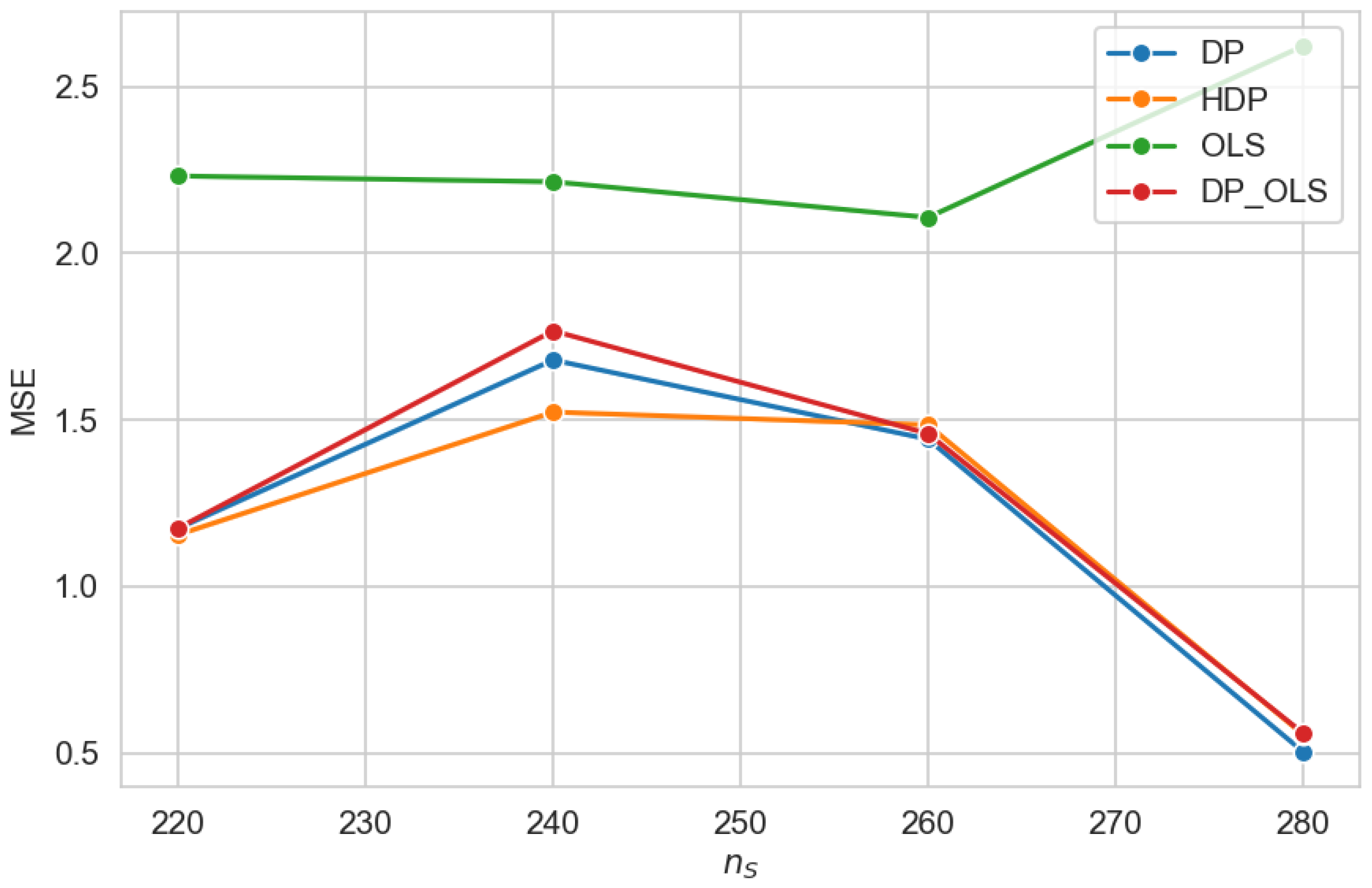
In this subsection, we investigate the effect of the source-domain sample size $n_S$ on estimation performance, while all other experimental settings remain fixed as specified at the beginning of this section. Specifically, the target-domain sample size is fixed at $n_T=10$, and the source-domain sample size varies over a moderate range given by the closed interval $n_S\in [220,280]$. The mean squared error (MSE) is used to evaluate the performance of the proposed HDP estimator in comparison with DP, OLS, and DP_OLS. The corresponding results are reported in Figure 1.

Figure 1 shows that the HDP estimator achieves the lowest MSE when the source-domain sample size is moderate, particularly for $220\le n_S\le 260$. In this regime, HDP consistently outperforms DP and DP_OLS, while the performance gap gradually diminishes as $n_S$ increases. When the source-domain sample size becomes sufficiently large, the performance of HDP converges to that of the two pooled estimators, suggesting that the benefit of carefully weighting source information is partially offset by the sheer volume of source data.

Across all values of $n_S$, the OLS estimator exhibits a substantially higher MSE than the other methods, highlighting its inability to effectively leverage source-domain information. Overall, these results indicate that the proposed HDP estimator is particularly effective in regimes with moderate source sample sizes.

5.1.2. Correlation Experiment

This subsection investigates the impact of feature correlation on estimation performance. In particular, we examine how varying the correlation coefficient between covariates affects the effectiveness of information transfer from the source domain to the target domain.

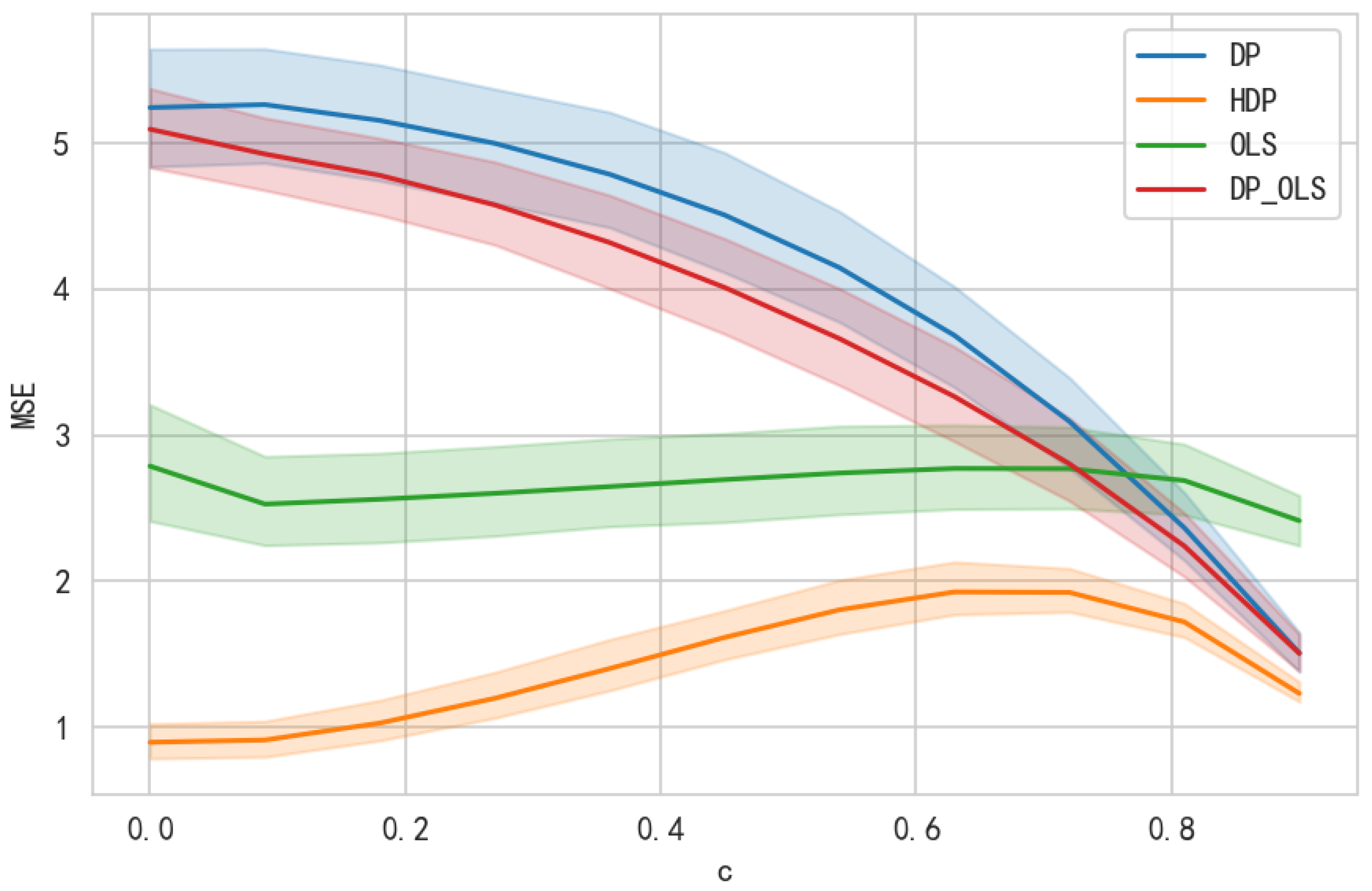
The source-domain sample size is fixed at $n_S=100$, and the target-domain sample size is fixed at $n_T=8$. The correlation coefficient c between $X_1$ and $X_2$ is varied over the interval $[0,0.9]$, while all other data-generating settings remain unchanged. For each value of c, the results are averaged over 200 independent Monte Carlo replications. The mean squared error (MSE) is used as the evaluation metric. The corresponding results are reported in Figure 2.

As shown in Figure 2, the performance of all methods is influenced by the correlation structure of the covariates. The proposed HDP estimator consistently achieves lower MSE than DP, OLS, and DP_OLS across the full range of correlation values, demonstrating robustness to changes in feature dependence.

Notably, the MSE curves exhibit a non-monotonic pattern as the correlation coefficient increases. When the correlation is low ($c<0.3$), both DP and DP_OLS suffer from relatively large estimation errors, indicating limited transferability between weakly related features. As the correlation increases, their performance improves, yet they remain inferior to HDP.

For the HDP estimator, moderate levels of correlation may introduce additional estimation variability due to the interaction between heterogeneous noise variances and partially aligned feature structures. However, in high-correlation regimes ($c>0.8$), the MSE of HDP decreases, suggesting that strong feature similarity enables more effective utilization of source-domain information for variance reduction. Overall, these results highlight the advantage of the HDP estimator in accommodating heterogeneous noise structures across a wide range of correlation settings.

5.1.3. Residual-Based Weighting

This subsection investigates a practical weighting strategy based on residual information, motivated by scenarios in which observation-level noise variances are unknown and the HDP estimator is, therefore, infeasible. To this end, we consider a residual-based weighted data-pooling approach (WDP), in which observation-specific weights are constructed from squared residuals obtained via preliminary ordinary least squares fits on the source and target domains. This procedure yields a heteroscedasticity-aware pooled estimator without requiring explicit knowledge of the underlying noise variances and can be viewed as an implementable approximation of variance-based weighting. Specifically, domain-specific residual variances are estimated via OLS fits on the source and target samples, and the resulting squared residuals are used to construct diagonal weighting matrices in a pooled weighted least squares (WLS) estimator.

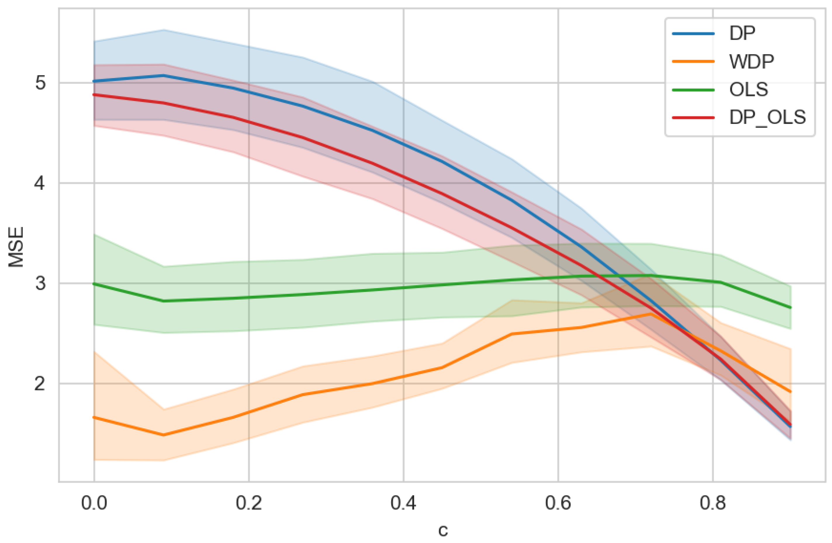
The experimental setting follows the previous configuration, where the correlation coefficient c between newly introduced and existing target-domain features serves as the independent variable, and MSE on the test set is used for evaluation. The performance of four estimators, DP, WDP, OLS, and DP_OLS, is summarized in Figure 3. We note that HDP estimator is not included here, as its behavior under varying correlation structures has already been examined in Section 5.1.2. The purpose of this experiment is to evaluate whether residual-based weighting can partially recover the benefits of variance-aware pooling in the absence of oracle variance information.

Overall, both DP and DP_OLS exhibit decreasing MSE as the correlation increases, reflecting the growing effectiveness of naive data pooling when the new and existing features become strongly aligned. In contrast, the OLS estimator remains relatively insensitive to feature correlation, showing limited variation across different settings. The residual-weighted estimator achieves the lowest MSE under low to moderate correlation levels, indicating that adaptive weighting based on residual information can effectively mitigate heteroscedastic effects in this regime.

When the correlation becomes sufficiently large, the performance gap between residual-weighted pooling and unweighted pooling narrows. In this case, the strong linear dependence between features enhances the utility of pooled data, reducing the relative benefit of residual-based reweighting. Nevertheless, across a broad range of correlation values, the residual-weighted approach remains competitive and demonstrates clear advantages in scenarios characterized by weak to moderate feature dependence and heteroscedastic noise.

5.1.4. The Impact of $n_T$ on Transfer Gain

Unlike the previous subsections, which focus on estimation accuracy measured by prediction error, this subsection directly investigates the effect of the target-domain sample size on the empirical transfer gain achieved by data pooling. The goal is to quantify when and to what extent incorporating source-domain information leads to performance improvement over target-only estimation.

To this end, the source sample size is fixed at $n_S=100$, while the target sample size $n_T$ varies from 5 to 30. The data-generating process follows a linear regression model, $y=2+2X_1-2X_2+w$, where the target-domain model is deliberately misspecified by retaining only $X_1$, while the source-domain model remains correctly specified. For each value of $n_T$, the empirical transfer gain is evaluated using a fixed test set of size $n_{\mathrm{test}}=1000$, and the results are averaged over 200 independent repetitions.

The transfer gain for the i-th repetition is given by

$$G_i={\displaystyle \frac{1}{n_{\mathrm{test}}}}\sum _{(X,y)\in D_{\mathrm{test}}}\left[{(y-X{\widehat{\beta }}_T)}^2-{(y-X{\widehat{\beta }}_{\alpha })}^2\right],$$

(13)

and the reported empirical transfer gain corresponds to the average of $G_i$ across all repetitions. The specific execution process is listed in Algorithm 2.

Algorithm 2 Empirical Transfer Gain Algorithm

Input: Number of iterations L, test dataset $D_{\mathrm{test}}$ 1:     for $i=1,\dots ,N$ do 2:             Randomly sample $D_S$ and $D_T$ 3:             Calculate ${\widehat{\beta }}_a$ and ${\widehat{\beta }}_T$ 4:             Calculate empirical transfer gain using Formula (13) 5:     end Output: Average of all $G_i$

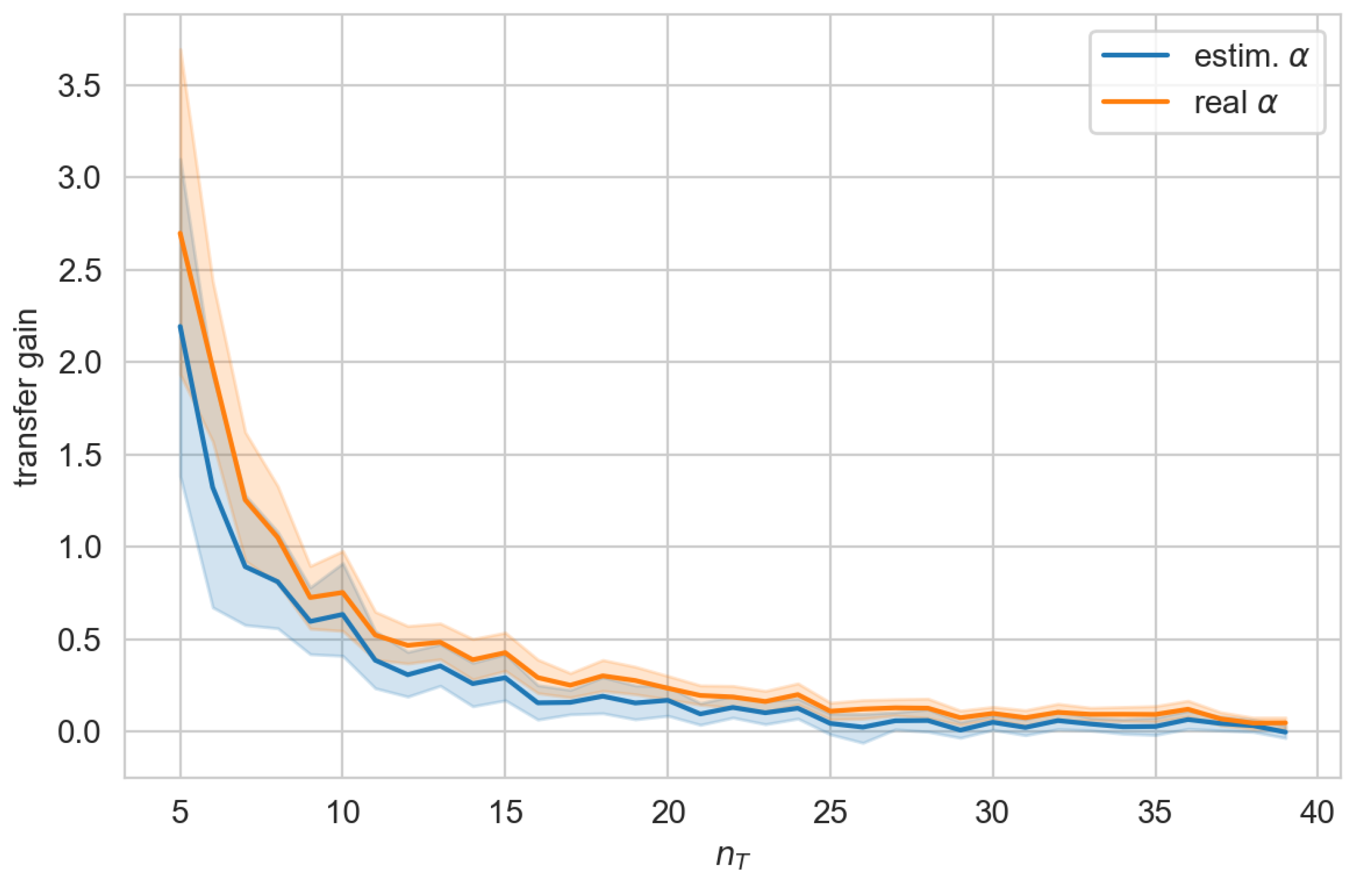
The empirical results in Figure 4 show that the transfer gain remains non-negative across all target sample sizes, which is consistent with the theoretical guarantee in Theorem 1. The gain attains its maximum when the target sample size is small and gradually decays toward zero as $n_T$ increases. This pattern reflects the diminishing error reduction effect of data pooling as the target-only estimator becomes more stable with an increasing sample size. Moreover, the transfer gain obtained using the estimated weighting parameter closely follows the oracle-based curve, indicating that the proposed data-driven estimation of $\alpha$ provides an accurate and effective approximation to the ideal variance-based weighting scheme.

5.1.5. The Impact of $n_S$ and $n_T$ Simultaneously

To examine the combined influence of source and target sample sizes on transfer performance, we implement a grid-based simulation that simultaneously adjusts $n_S$ and $n_T$ across a range of practical values. The source domain sample size is set to $n_S\in \{50,100,150,200,250,300\}$, and the target domain sample size is set to $n_T\in \{5,10,15,20,25,30\}$. Heteroscedastic noise is generated with variances uniformly sampled from $\mathcal{U}(0.1,2)$ for both domains, and feature mismatch is constructed by reducing the source feature dimension. The definition of transfer gain is consistent with that in Section 5.1.4.

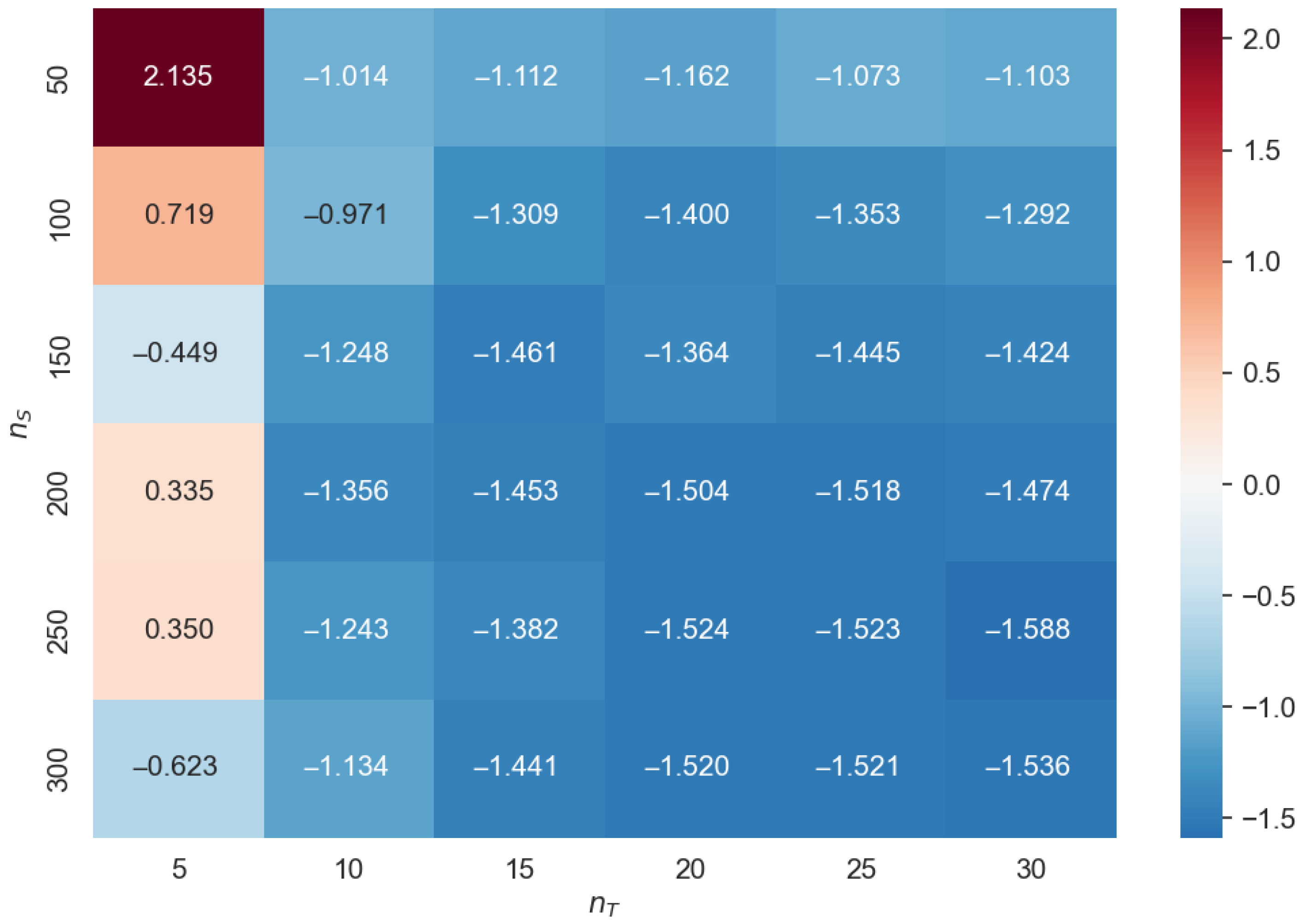
As illustrated in Figure 5, the maximum positive transfer gain reaches 2.135 when $n_S=50$ and $n_T=5$, followed by a gain of 0.719 for $n_S=100$ and $n_T=5$; all other combinations yield negative transfer gains, with the minimum value of −1.588 observed at $n_S=250$ and $n_T=30$. The HDP estimator delivers a significant positive transfer gain only in the regime where the target domain is extremely data-scarce ($n_T=5$) and the source domain sample size is small to moderate ($n_S\le 100$). As $n_T$ increases beyond 5, the transfer gain immediately turns negative and remains stable at approximately −1.0 to −1.6 across all $n_S$ values; when $n_S$ exceeds 100 (even for $n_T=5$), the positive gain diminishes rapidly, with $n_S=150$ already yielding a negative gain of −0.449. These patterns confirm that the relative scale of $n_S$ and $n_T$ is the dominant factor for transfer effectiveness: HDP excels in scenarios where target data is highly limited and source data is moderately available, while excessive source data or sufficient target data leads to a negative transfer due to an amplified feature mismatch bias and a reduced reliance on source information.

5.2. Case Study

This section extends the theoretical analysis to real-life datasets, aiming to examine the practical performance of the proposed method under heterogeneous noise and limited target-domain samples. By considering a diverse collection of benchmark regression tasks with varying dimensionality and sample sizes, the following experiments assess whether the empirical performance of different estimators aligns with the theoretical transfer gain and robustness properties established earlier.

5.2.1. Comparison of Four Methods Under Different Dataset Settings

The empirical evaluation is conducted on nine multivariate regression datasets from the UCI repository, with dataset statistics summarized in

Table 1. Dataset statistics.

Dataset	${\mathbf{n}}_{\mathbf{total}}$	${\mathbf{n}}_{\mathbf{S}}$	${\mathbf{n}}_{\mathbf{T}}$	${\mathbf{n}}_{\mathbf{test}}$	${\mathbf{d}}_{\mathbf{T}}$	#Runs
concrete	1030	114	38	103	8	21
energy	768	114	38	76	8	15
kin40k	40,000	114	38	4000	8	50
parkinsons	5875	150	50	587	20	50
pol	15,000	168	56	1500	26	50
protein	45,730	117	39	4573	9	50
pumadyn32nm	8192	186	62	819	32	50
skillcraft	3338	147	49	333	19	50
sml	4137	156	52	413	22	50

. For each dataset, samples are partitioned into source, target, and test sets according to predefined sizes. To simulate an incremental feature setting, a subset of covariates is removed from the source domain and treated as newly introduced features in the target domain. These features are selected based on their Pearson correlation with the response variable, ensuring that the OLS estimator operates on the most informative covariates. Model performance is assessed using RMSE computed on an independent test set.

To investigate the impact of data availability on transfer performance, two distinct sampling regimes are considered, following common practice in the transfer learning literature.

Small data regime: In the small data setting, the source dataset and the test dataset are fixed across runs, while multiple disjoint target datasets of limited size are repeatedly sampled. Each sampled target dataset is used to train the transfer learning estimators, as well as the OLS baseline. This regime is designed to mimic scenarios in which only a small amount of target-domain data is available, such that estimation performance is primarily dominated by variance. By repeatedly resampling the target data, we evaluate the stability and sensitivity of different methods under severe target-data scarcity.

Large data regime: In the large data setting, for each dataset, a fixed proportion (10%) of the samples is randomly drawn as the test set in each run. The target-domain sample size is fixed at a moderate level, as reported in Table 1, while the source-domain sample size is specified accordingly for each dataset. Depending on the dataset, this procedure can result in either relatively large source datasets or moderately sized target datasets. This regime allows us to examine how transfer performance evolves as the overall data availability increases and whether the benefits of data pooling persist in data-rich settings.

All experiments are repeated multiple times with independent random splits. The reported results correspond to the mean RMSE, together with one standard deviation, providing a quantitative summary of both predictive accuracy and performance stability across different datasets and sampling regimes.

Under the small data regime (

Table 2. RMSE of four methods under a small data regime.

Dataset	OLS	DP	DP_OLS	HDP
concrete	14.7 ± 2.5	14.4 ± 3.02	14.7 ± 2.5	14.5 ± 2.4
energy	3.4 ± 0.395	3.63 ± 0.36	3.4 ± 0.395	3.62 ± 0.177
kin40k	1.14 ± 0.0846	1.06 ± 0.0375	1.14 ± 0.0846	1.09 ± 0.0656
parkinsons	18.3 ± 5.95	10.8 ± 0.531	18.3 ± 5.95	11 ± 0.44
protein	0.851 ± 0.141	0.713 ± 0.0353	0.851 ± 0.141	0.733 ± 0.0487
pumadyn32nm	1.47 ± 0.171	1.09 ± 0.0302	1.47 ± 0.171	1.12 ± 0.0489
skillcraft	0.344 ± 0.0501	0.258 ± 0.0091	0.344 ± 0.0501	0.265 ± 0.0124
sml	3.4 ± 0.752	2.72 ± 0.482	3.4 ± 0.752	2.84 ± 0.62

), HDP yields lower RMSE than the OLS estimator in most datasets, with the exception of the energy dataset where all methods achieve comparable performance. Compared with DP_OLS, the improvement offered by HDP is particularly evident in datasets such as parkinsons, pumadyn32nm, and skillcraft, where accounting for heterogeneous noise leads to a noticeable reduction in the estimation error. When compared with naive DP, the performance advantage of HDP is dataset-dependent but generally manifests as comparable or slightly lower RMSE.

As the target sample size increases under the large data regime (

Table 3. RMSE of four methods under large data regime.

Dataset	OLS	DP	DP_OLS	HDP
concrete	11 ± 1	11.1 ± 0.53	11 ± 1	11.3 ± 0.54
energy	2.95 ± 0.358	3.12 ± 0.35	2.95 ± 0.358	3.16 ± 0.34
parkinsons	11.1 ± 1.16	9.31 ± 0.225	11.1 ± 1.16	9.33 ± 0.235
pol	54.2 ± 20.3	30.7 ± 0.449	54.2 ± 20.3	30.8 ± 0.527
pumadyn32nm	1.21 ± 0.0732	1 ± 0.0301	1.21 ± 0.0732	1.01 ± 0.0298
skillcraft	0.317 ± 0.136	0.267 ± 0.0397	0.317 ± 0.136	0.265 ± 0.0299
sml	2.87 ± 0.919	2.2 ± 0.253	2.87 ± 0.919	2.2 ± 0.286

), performance differences among the four methods become less pronounced. Nevertheless, HDP continues to outperform or closely match the OLS estimator in several datasets, including parkinsons, pol, pumadyn32nm, and skillcraft. Relative to DP and DP_OLS, HDP remains competitive and often achieves stable performance without exhibiting large degradation.

Overall, the empirical results suggest that the transfer gain, as defined in Section 4, is predominantly non-negative across most datasets and sampling regimes, in the sense that HDP rarely underperforms the OLS baseline in terms of RMSE. These observations are consistent with the theoretical generalization error analysis developed earlier and support the applicability of heteroscedasticity-aware data pooling in regression problems with heterogeneous noise structures.

5.2.2. Comparison of Four Methods on a Single Dataset

To provide a more fine-grained empirical understanding of the proposed transfer learning method, we conduct a detailed comparison of four estimators on individual real-world datasets. Unlike aggregated evaluations across multiple tasks, this subsection focuses on single-dataset analyses in order to clearly illustrate how transfer learning performance varies with the target-domain sample size under heterogeneous noise and partial feature overlap.

We select three representative regression datasets from the UCI repository: 3D Road Network, Airfoil, and Breastcancer. These datasets differ substantially in scale, noise characteristics, and feature–response relationships, making them suitable benchmarks for evaluating robustness and transfer gain in practical settings.

Table 4. Variables of source domain data and target domain data in each dataset.

Dataset	${\mathit{X}}_1$	${\mathit{X}}_2$	y
3D Road Network	OSM_ID	Longitude	Altitude
Airfoil	Frequency	Chord-length	Scaled sound pressure
Breastcancer	Time	Fractal_dimension3	Outcome

summarizes the variables used in the source and target domains for each dataset. In all cases, the feature $X_1$ is available only in the target domain, while $X_2$ is shared by both the source and target domains, representing a typical transfer learning scenario with incremental feature availability.

The strength of association between covariates and the response variable is reported in

Table 5. Pearson correlation coefficients.

Dataset	$\mathbf{cor}({\mathbf{X}}_1,\mathbf{y})$	$\mathbf{cor}({\mathbf{X}}_2,\mathbf{y})$	${\mathbf{n}}_{\mathbf{test}}$	${\mathbf{n}}_{\mathbf{S}}$	#Runs
3D Road Network	0.106	0.042	43,000	100	115
Airfoil	−0.390	−0.236	150	100	70
Breastcancer	−0.346	0.287	20	100	117

through Pearson correlation coefficients. Across all three datasets, the target-only feature $X_1$ exhibits a stronger correlation with the response variable y than the shared feature $X_2$. This implies that models trained solely on the source domain cannot exploit the most informative covariate and, therefore, are expected to suffer from higher variance or bias when the target sample size is small. Such a setting is particularly favorable for transfer learning methods that can effectively integrate source information while adapting to newly introduced target-specific features.

For each dataset, the source and test sets are fixed, while target datasets of varying sizes, $n_T$, are sampled. Specifically, $n_T$ ranges from the 8th to the 30th data point, and for each value of $n_T$, the experiment is repeated multiple times with independent random sampling. The test set remains unchanged throughout to ensure a fair comparison across different target sample sizes. Model performance is evaluated using MSE computed on the test set. Since the response variable y is measured on a fixed scale within each dataset, the MSE values are directly comparable across methods for the same task, and a lower MSE indicates better predictive accuracy.

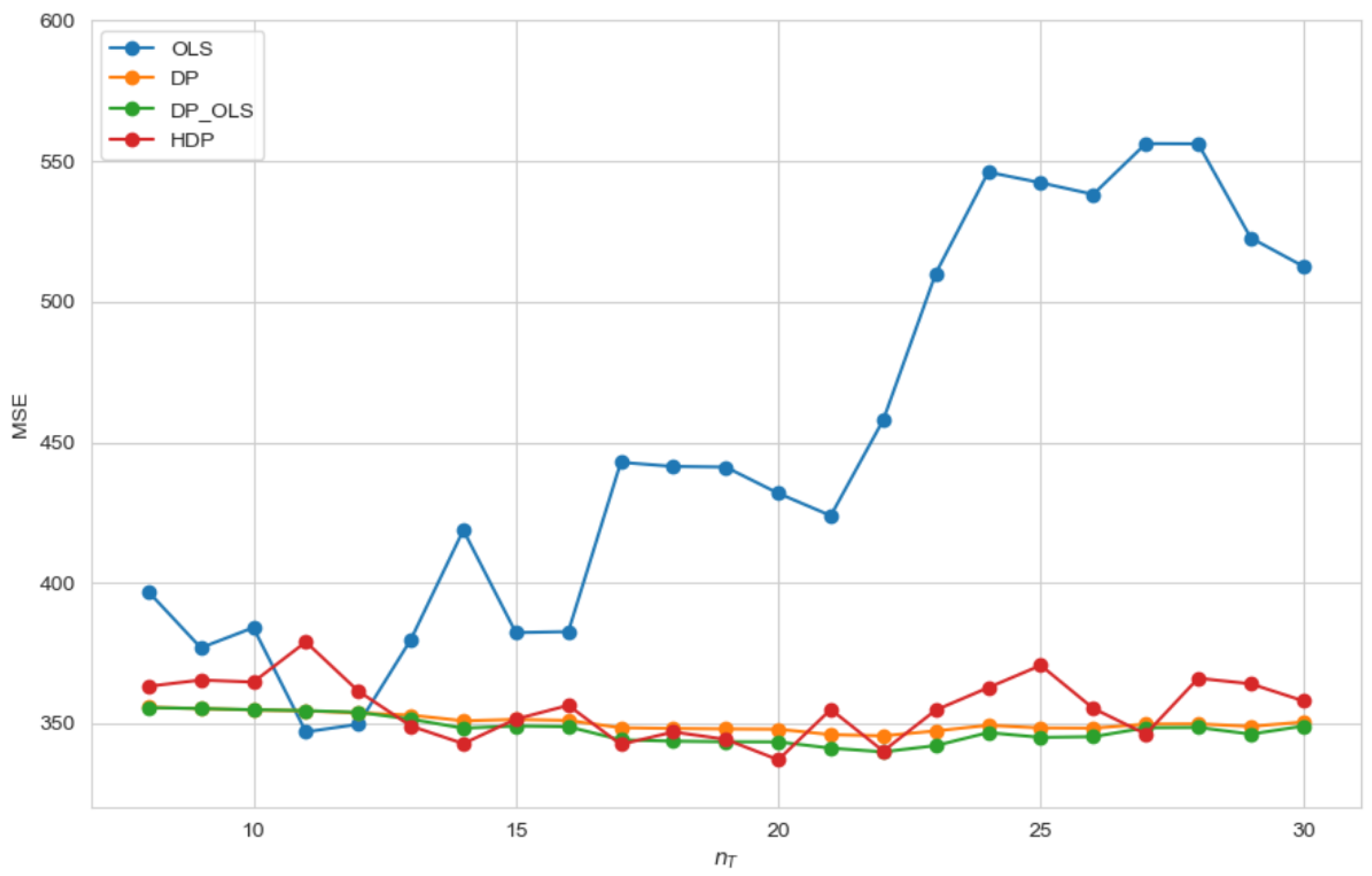
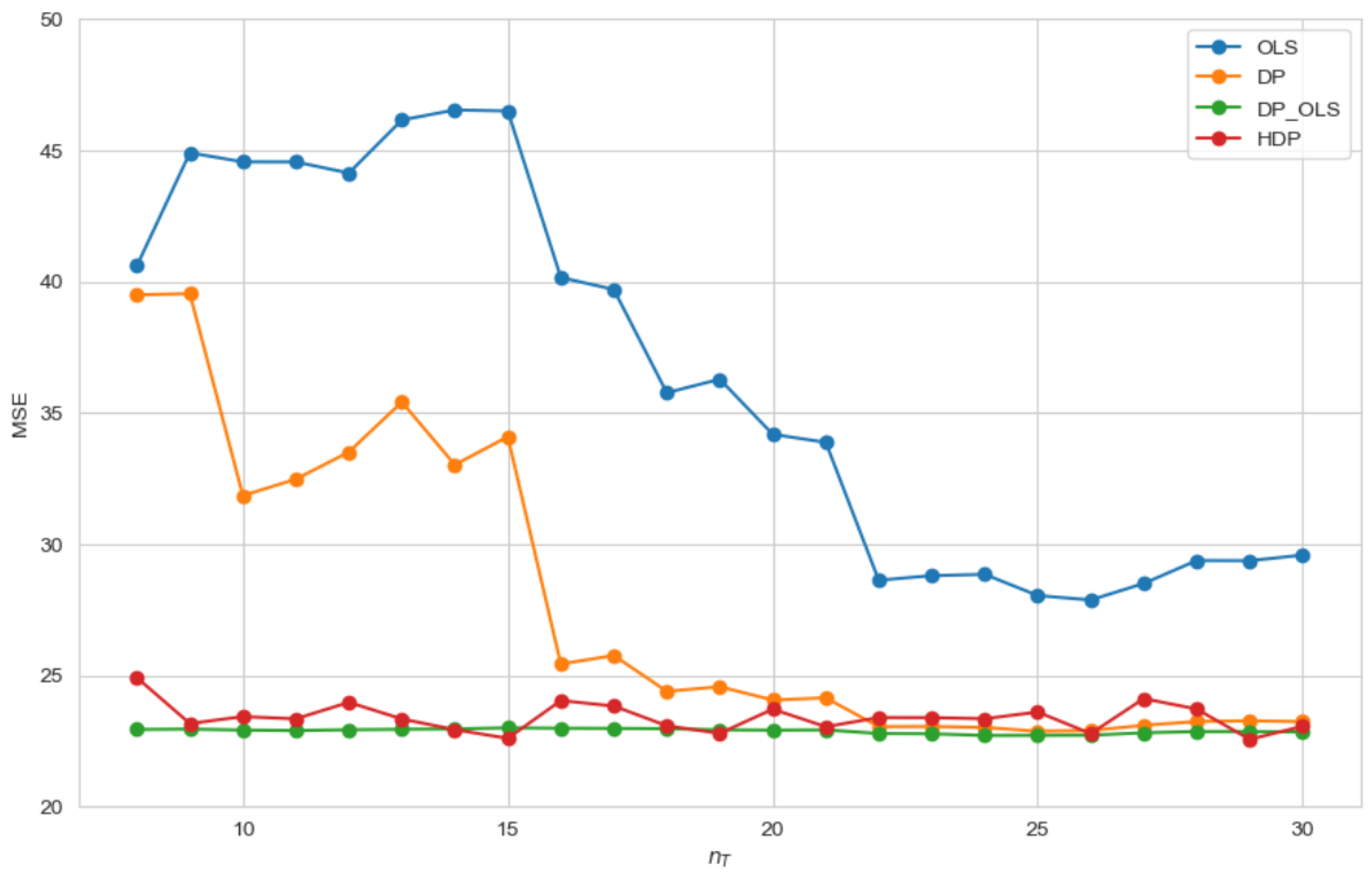
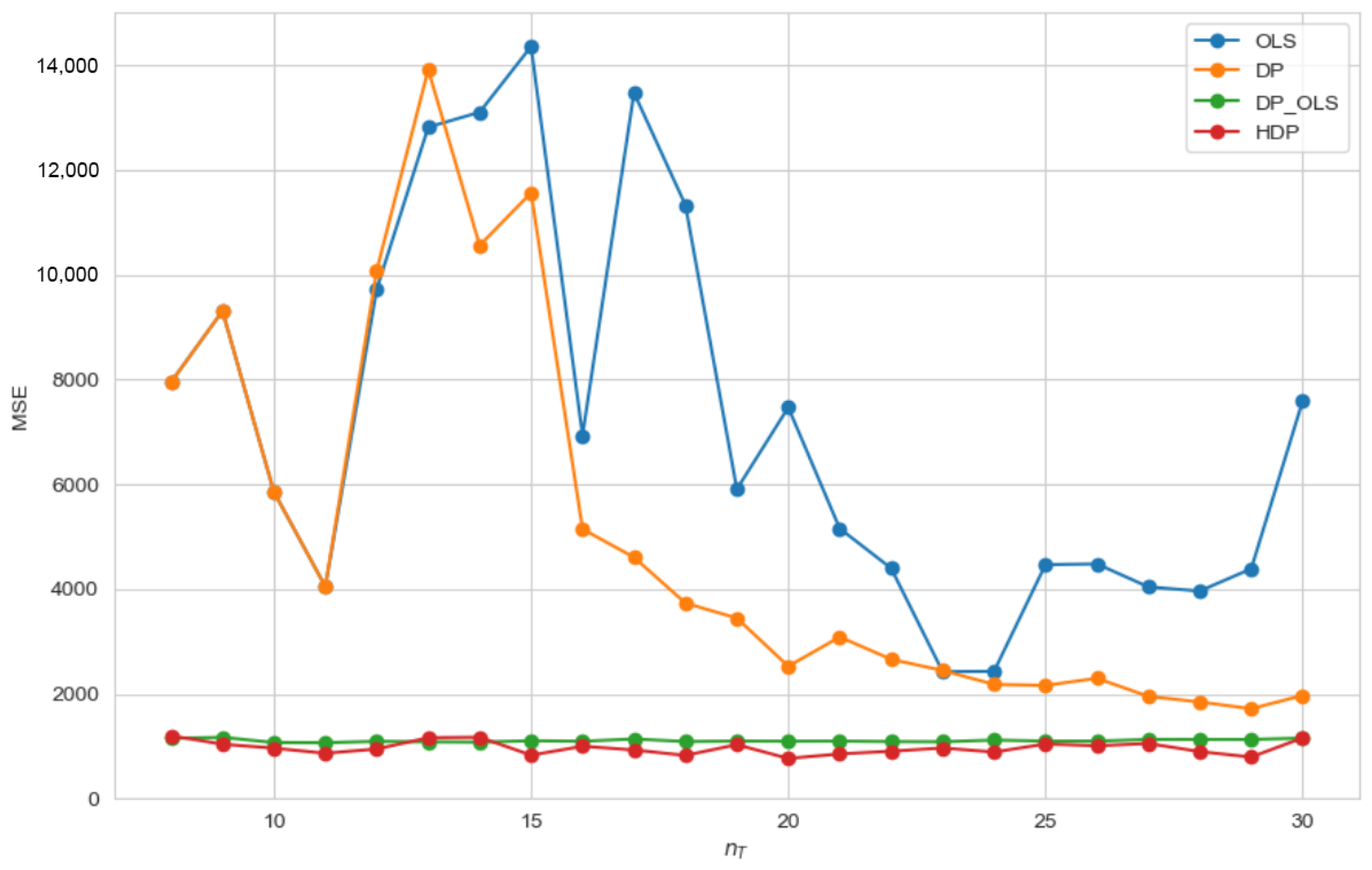
The empirical results for the 3D Road Network, Airfoil, and Breastcancer datasets are illustrated in Figure 6, Figure 7, and Figure 8, respectively. For the 3D Road Network dataset, the OLS estimator exhibits substantial fluctuations when $n_T$ is small, with significantly higher MSE compared to the transfer learning methods. This behavior reflects the sensitivity of OLS to heteroscedastic noise and limited target-domain samples. In contrast, HDP and DP_OLS maintain relatively low and stable MSE values across different target sample sizes, demonstrating improved robustness.

A similar pattern is observed in the Airfoil dataset. Although the performance of OLS improves as $n_T$ increases, it consistently underperforms compared to transfer-based estimators, particularly in the small-sample regime. Both DP and DP_OLS achieve stable MSE values across the entire range of $n_T$, indicating their effectiveness in handling heteroscedasticity and exploiting source-domain information.

For the Breastcancer dataset, the advantage of HDP is most pronounced when $n_T$ is small. In this regime, its MSE is substantially lower than that of OLS and DP, confirming its ability to achieve significant variance reduction under strong heteroscedastic effects. As $n_T$ increases, the performance gap narrows, yet the proposed estimator remains competitive. DP shows reasonable performance for a small $n_T$ but gradually deteriorates as the target sample size grows, eventually approaching the behavior of OLS, whereas DP_OLS maintains stable accuracy throughout.

Overall, these empirical findings are consistent with the theoretical analysis presented in Section 4. When the target-domain sample size is limited, the baseline estimator suffers from high variance, and the transfer gain achieved by incorporating source-domain information is maximized. As $n_T$ increases, the marginal benefit of transfer learning diminishes, but robust transfer-based methods continue to outperform or match classical estimators. This confirms that the proposed approach is particularly advantageous in small-sample, heteroscedastic settings commonly encountered in real-world applications.

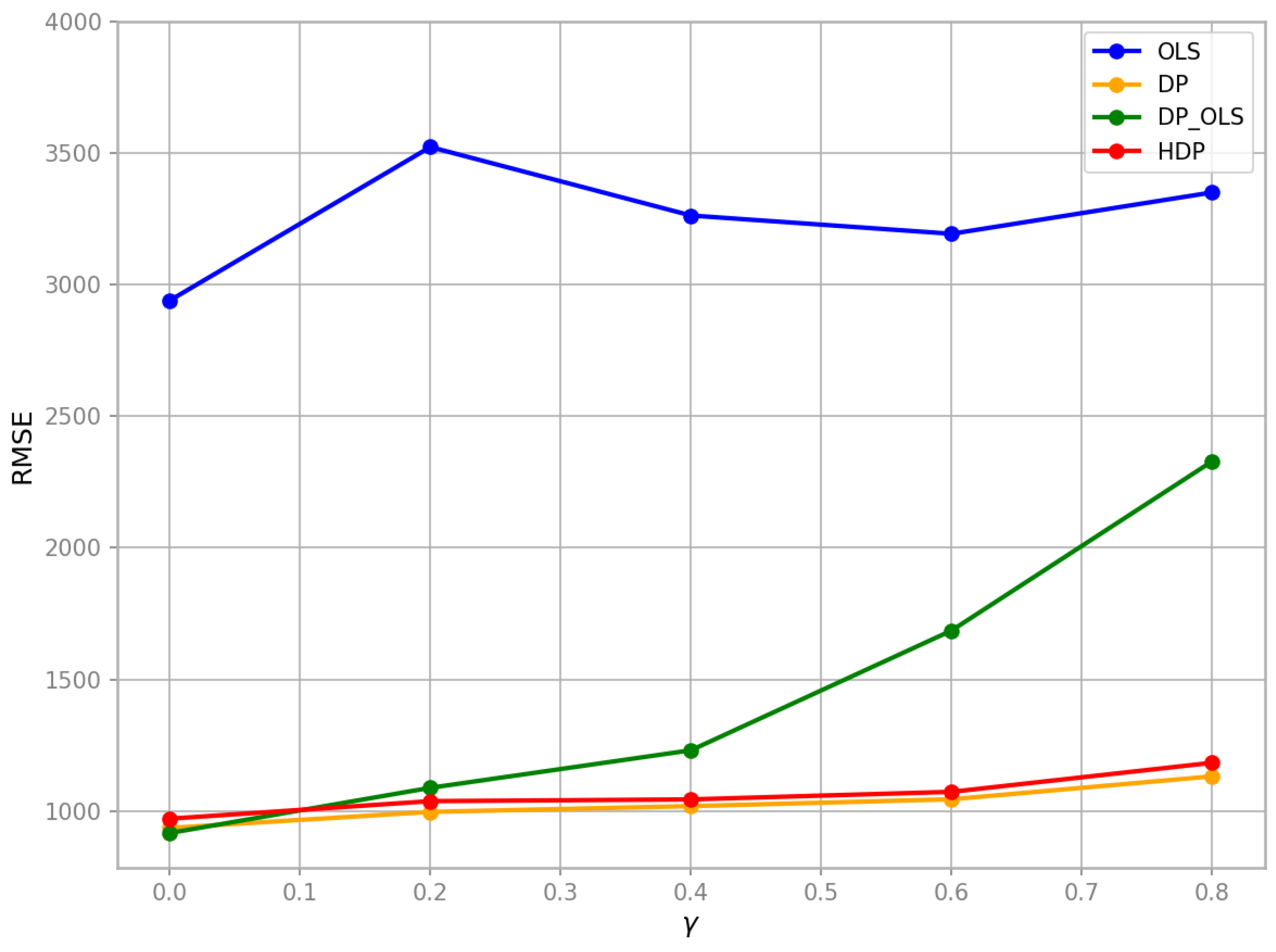
5.2.3. Sensitivity Analysis on Shared Feature Proportion

To investigate the robustness of different transfer learning methods under feature misalignment, we conducted a sensitivity analysis using the UCI Breastcancer dataset. The dataset was randomly split into a training set and a test set, with 50 samples selected as the target domain and 200 samples as the source domain. Feature misalignment was simulated by reducing the source domain features to a certain proportion of the target domain dimension. We denote the feature misalignment level as $\gamma \in [0,1]$, where $\gamma =0$ indicates full feature alignment, and larger values of $\gamma$ correspond to more severe feature misalignment. The analysis was conducted at $\gamma =0, 0.2, 0.4, 0.6, 0.8$. Performance is evaluated using RMSE.

The results are shown in Figure 9. OLS exhibited strong sensitivity to feature misalignment, with RMSE increasing noticeably as $\gamma$ increased, indicating that relying solely on target domain samples leads to rapid performance degradation when the source domain contains fewer features. In contrast, DP maintained relatively stable RMSE values across different levels of $\gamma$, demonstrating that distribution correction and weighting effectively mitigate the impact of missing source domain features. DP_OLS showed considerable performance fluctuation, suggesting that the simple combination of source and target domains via OLS is vulnerable to feature misalignment.

HDP demonstrated the best robustness among the four methods, with only a moderate increase in RMSE as $\gamma$ increased, indicating that its weighted robust strategy effectively preserves predictive accuracy under severe feature misalignment. Notably, under high levels of feature misalignment, HDP consistently outperformed OLS and DP_OLS, highlighting its superiority in handling feature inconsistency between domains. These results suggest that HDP and DP are relatively insensitive to feature misalignment and can effectively leverage source domain information, thereby enhancing the interpretability of the experimental findings and supporting their applicability in practical transfer learning scenarios.

6. Conclusions

In terms of transfer learning, the existing homogeneous transfer learning methods across domains assume that the dimensions of the source and target datasets are the same and often assume homoscedasticity in linear regression. To address both of the above issues simultaneously, in this work, we have proposed a method for heterogeneous transfer learning that allows heteroscedasticity in linear regression and the different dimensions of the source and target datasets. The theoretical property of the proposed heteroscedasticity data-pooling estimator shows an upper bound for its generalization error and its robustness against adverse transfer. Extensive simulation experiments confirmed the effectiveness of the proposed algorithm. The empirical study in the UCI datasets demonstrates that the proposed methodology performs better than the baseline estimator. In summary, the methodology in this paper effectively addresses key challenges in homogeneous transfer learning with homoscedasticity in the linear regression, yielding satisfactory results in heterogeneous transfer learning for linear regression with heteroscedasticity. However, this paper relies on several assumptions, such as $d_S<d_T$ and the incremental features $X_{ij}^{″}\stackrel{\mathrm{i}.\mathrm{i}.\mathrm{d}.}{\sim }N(0,1)$. When these conditions are not satisfied in practice, exploring more general settings beyond these assumptions constitutes an interesting direction for future research. In addition, we can also delve more deeply into the theoretical foundations, extend this algorithm to other models, consider differences between conditional distributions in source and target datasets, and further explore practical application scenarios.