Article

Algebraic Reduction and Periodic Solvability in a Coupled Ternary Rational System

by
Ahmed Ghezal
1,*,
Ahmed A. Al Ghafli
2,* and
Hassan J. Al Salman
2
1
Department of Mathematics, Abdelhafid Boussouf University of Mila, Mila 43000, Algeria
2
Department of Mathematics and Statistics, College of Science, King Faisal University, Hofuf 31982, Alahsa, Saudi Arabia
*
Authors to whom correspondence should be addressed.
Mathematics 2026, 14(8), 1396; https://doi.org/10.3390/math14081396
Submission received: 14 March 2026 / Revised: 12 April 2026 / Accepted: 16 April 2026 / Published: 21 April 2026
(This article belongs to the Special Issue Research on Dynamical Systems and Differential Equations, 2nd Edition)

Abstract

In this paper, we investigate a new class of three-component nonlinear rational difference equations of the second order characterized by structured periodic interactions. Through a carefully designed algebraic transformation and the introduction of suitable auxiliary sequences, the original nonlinear model is converted into an equivalent periodic scheme of order six. This reformulation enables the complete determination of explicit solution formulas in closed form. We establish precise conditions under which the solutions remain well defined and analytically tractable. A series of illustrative numerical experiments reveals a wide spectrum of dynamical behaviors, ranging from oscillatory patterns to various modes of convergence.

1. Introduction

The theory of difference equations and systems of difference equations has witnessed remarkable development over the last few decades, owing to its fundamental role in modeling discrete-time phenomena arising from diverse scientific disciplines such as biology, physics, engineering, economics, time series analysis, and control theory (e.g., [1,2,3,4,5,6,7,8,9]). In particular, nonlinear rational difference equations and their higher-order systems have attracted sustained interest, since they are capable of exhibiting a wide range of rich dynamical behaviors, including periodicity, boundedness, oscillation, and convergence, while at the same time admitting, in certain cases, explicit closed-form solutions [10,11,12,13,14,15,16,17]. The search for solvable nonlinear difference equations is of major importance, as explicit solution formulas provide a powerful analytical tool for understanding the qualitative behavior of solutions (see, e.g., [18,19,20,21,22,23,24,25,26,27,28]). Such formulas allow researchers to precisely describe the long-term dynamics, detect periodic patterns, and determine the limiting behavior without relying solely on numerical simulations. Consequently, identifying new classes of solvable systems and extending known solvable models to higher dimensions or more general structures remain a central topic in modern difference equation theory. One of the early motivations in this direction can be traced back to the study of the nonlinear rational difference equation:
u m + 1 = a u m u m 1 b u m c + d ,
where the parameters a, b , and the initial conditions u l ,   l = 0 , 1 , are assumed to be nonzero real numbers, while the remaining parameters c, d, are arbitrary real numbers, which was investigated in connection with the qualitative behavior of higher-order rational difference equations. In particular, Elabbasy, et al. [29] systematically analyzed a broad class of higher-order recursive sequences, where they established conditions for the well-definedness of solutions and explored the qualitative behavior of the corresponding dynamics, including periodicity and boundedness. These studies highlighted the effectiveness of appropriate algebraic transformations in reducing nonlinear equations to more tractable forms. Inspired by this line of research, attention was subsequently directed toward coupled systems of rational difference equations. Haddad et al. [30] considered the second-order system:
u m + 1 = a 1 u m v m 1 v m c 1 + c 2 , v m + 1 = a 2 v m u m 1 u m c 2 + c 1 , m N 0 ,
where the parameters a i , i = 1 , 2 , and the initial conditions u l ,   v l ,   l = 0 , 1 , are assumed to be nonzero real numbers, while the remaining parameters c i , i = 1 , 2 , are arbitrary real numbers, and established its solvability by reducing it to a system of linear difference equations through appropriate substitutions. Moreover, they investigated the periodic nature and the limiting behavior of its solutions, thereby extending earlier results for scalar equations to a fully coupled two-dimensional framework. Later, Yazlık et al. [31] further generalized this system by allowing the coefficients to be periodic sequences, leading to a class of higher-order systems with period-two coefficients,
u m + 1 = a 1 , m u m v m 1 v m c 1 , m + c 2 , m + 1 , v m + 1 = a 2 , m v m u m 1 u m c 2 , m + c 1 , m + 1 , m N 0 ,
where the initial conditions u l , v l ,   l = 0 , 1 , are assumed to be nonzero real numbers, and a 1 , m , a 2 , m , c 1 , m , c 2 , m m is two periodic sequence of real numbers. Their analysis demonstrated that even in the presence of time-dependent parameters, explicit closed-form solution formulas can still be obtained, and the qualitative behavior of solutions can be completely characterized under suitable conditions. This contribution marked an important step toward understanding solvable nonlinear systems with nonconstant (periodic) coefficients. Further progress was achieved by Touafek and Al-Juaid [32], who introduced a more general second-order rational system by incorporating additional linear terms in both the denominators and the numerators,
u m + 1 = a 1 u m v m 1 v m b 1 v m 1 c 1 + b 2 u m + c 2 , v m + 1 = a 2 v m u m 1 u m b 2 u m 1 c 2 + b 1 v m + c 1 , m N 0 .
The parameters a i , i = 1 , 2 , and the initial conditions u l ,   v l ,   l = 0 , 1 , are assumed to be nonzero real numbers, while the remaining parameters b i , c i , i = 1 , 2 , are arbitrary real numbers. They derived explicit closed-form expressions for the solutions and conducted a comprehensive analysis of periodicity and the limiting behavior, showing that their model substantially generalizes several known systems in the literature. Moreover, their approach emphasized the unifying role of algebraic transformations in uncovering solvable structures within apparently complex nonlinear systems. Motivated by these developments, it is natural to ask whether such solvability and qualitative properties can be maintained when extending these models to higher-dimensional settings. Indeed, many real-world phenomena involve interactions among more than two components, and capturing such interactions requires the study of multidimensional systems of difference equations. In this paper, we propose and analyze a novel three-dimensional nonlinear system of second-order rational difference equations given by:
u m + 1 = a 1 u m v m 1 v m b 1 v m 1 c 1 + b 3 u m + c 3 , v m + 1 = a 2 v m w m 1 w m b 2 w m 1 c 2 + b 1 v m + c 1 , w m + 1 = a 3 w m u m 1 u m b 3 u m 1 c 3 + b 2 w m + c 2 , m N 0 ,
where the parameters a i , i = 1 , 2 , 3 , and the initial conditions u l ,   v l , w l ,   l = 0 , 1 , are assumed to be nonzero real numbers, while the remaining parameters b i , c i , i = 1 , 2 , 3 , are arbitrary real numbers. To further motivate the structure of system (1), it is important to emphasize that the proposed model is not introduced arbitrarily, but rather arises naturally as a cyclic extension of previously studied solvable systems. Indeed, earlier works have demonstrated that two-dimensional rational systems with cross interactions can be effectively reduced to linear forms via suitable transformations. The present system is constructed by preserving this interaction mechanism while extending it to a three-component cyclic framework, in which each variable depends on the previous state of another in a closed loop. This cyclic dependency represents a natural generalization of pairwise interactions to multi-component settings, which frequently arise in applications involving feedback mechanisms and interdependent processes. Moreover, the inclusion of linear terms alongside rational expressions is motivated by the need to balance nonlinearity with analytical tractability, thereby allowing the system to exhibit rich dynamical behavior while still admitting explicit solutions. Therefore, system (1) can be viewed as a structured and minimal higher-dimensional extension of known solvable models, specifically designed to preserve analytical solvability while capturing more complex interaction patterns. An important question that naturally arises is why it is necessary to consider a three-dimensional nonlinear system. The motivation extends beyond a mere increase in dimension. While two-dimensional systems capture pairwise interactions, many real-world processes involve cyclic dependencies among three or more components, in which the evolution of each variable is influenced by another in a closed-loop manner. Such structures cannot be fully captured within a two-dimensional framework. From a mathematical perspective, moving to three dimensions introduces fundamentally new dynamical features, including more intricate coupling mechanisms and richer periodic patterns. At the same time, preserving explicit solvability in this higher-dimensional setting is highly nontrivial. Therefore, the study of system (1) is motivated by the need to bridge the gap between tractable low- dimensional models and more realistic multi- component systems while maintaining analytical control through explicit solution formulas. This system represents a significant generalization of the previously studied one- and two-dimensional models. The proposed model naturally preserves and extends the cyclic interaction structure observed in earlier works and introduces a more intricate coupling mechanism among three interdependent sequences.
To further clarify the novelty of the proposed model in relation to existing works such as [29,30,31,32], it is important to highlight the fundamental differences in the structure and the nature of the interactions involved. The equations studied in [29] focus primarily on scalar higher-order dynamics, where the evolution depends on delayed terms of a single component. In contrast, systems such as [30,31,32] consider two-dimensional coupled interactions, where the dynamics are governed by pairwise relationships between two variables. The system proposed in this paper goes beyond these frameworks by introducing a three-component cyclic interaction, in which each variable depends on another in a closed- loop configuration. This type of interaction cannot be reduced to independent scalar equations or simple pairwise couplings and instead reflects a more intricate multi-component structure. From an application perspective, this allows the model to represent phenomena involving three interdependent processes evolving simultaneously, which are not adequately captured by one- or two-dimensional models. Moreover, the combination of cyclic coupling with rational nonlinearities and linear terms leads to a system that is structurally more complex while still admitting explicit closed- form solutions. This balance between increased dimensional complexity and analytical solvability constitutes a key novelty of the present work in comparison with the existing literature. The primary objectives of this study are to establish the solvability of the proposed system, derive explicit closed-form expressions for its solutions under appropriate conditions, and investigate the qualitative dynamics of well-defined solutions, including periodicity and asymptotic behavior. Furthermore, our results not only unify and generalize several existing contributions but also provide a systematic framework for the analysis of higher-dimensional solvable nonlinear difference systems.
The organization of the paper is as follows. Section 2 is devoted to the derivation of explicit solutions of the main system. Finally, concluding remarks and potential directions for future research are presented in the Section 3.

2. Main Result

In this section, we present a detailed procedure for obtaining explicit solutions of system (1). Our approach consists of two main steps: first, transforming the original system into an equivalent form that is more amenable to analysis, and second, applying established solution formulas to derive closed-form expressions for the transformed system. Before proceeding to the analysis of the nonlinear systems under consideration, it is useful to recall a classical result concerning nonhomogeneous first-order linear difference equations with variable coefficients. Such equations play a central role in the theory of difference equations, as many nonlinear equations and systems can be reduced to linear forms through appropriate algebraic transformations. In particular, explicit solution formulas for linear difference equations provide an essential analytical framework for deriving closed-form expressions and for studying the qualitative behavior of more involved models. The following lemma, which can be found in [33], presents the general solution of a nonhomogeneous first-order linear difference equation with real-valued coefficient sequences. This result will be repeatedly employed in the sequel to establish the solvability of the proposed system.
Lemma 1. 
Consider the first-order linear difference equation:
X m + 1 = α m X m + β m , m N 0 ,
where X 0 is a real initial value and α m , β m is a sequence of real numbers. In this case, the solution admits an explicit closed-form representation given by:
X m = k = 0 m 1 α k X 0 + l = 0 m 1 k = l + 1 m 1 α k β l , m N 0 ,
where we adopt the conventions: k = l m α k = 1 and k = l m β k = 0 whenever l > m . In the particular case where α m , β m = α , β for all m, the solution reduces to
X m = α m X 0 + α m 1 α 1 β i f α 1 X 0 + m β i f α = 1 , m N .
To gain deeper insight into the intrinsic dynamics of the considered cyclic system, it is crucial to examine how the mutual interactions among the sequences evolve over time. In particular, the symmetric structure of the system hints at the existence of underlying regularities and potential periodic behavior. The following lemma formalizes this intuition by demonstrating that the system can be reduced to higher-order relations and, moreover, exhibits a remarkable periodic pattern, ultimately leading to explicit closed-form expressions for all iterates.
Lemma 2. 
Let A m , B m , and C m be three sequences defined by the symmetric first-order cyclic system
A m + 1 = a 1 B m , B m + 1 = a 2 C m , C m + 1 = a 3 A m , m N 0 ,
where a 1 , a 2 , a 3 are nonzero constants and the initial values A 0 , B 0 , C 0 are nonzero. Then each sequence is periodic with period 6, and admits the closed-form representation
A 6 m + s = A 0 , s = 0 a 1 B 0 , s = 1 a 1 a 2 C 0 , s = 2 a 1 a 2 a 3 A 0 , s = 3 a 3 a 2 B 0 , s = 4 a 3 C 0 , s = 5 , B 6 m + s = B 0 , s = 0 a 2 C 0 , s = 1 a 2 a 3 A 0 , s = 2 a 2 a 3 a 1 B 0 , s = 3 a 1 a 3 C 0 , s = 4 a 1 A 0 , s = 5 , C 6 m + s = C 0 , s = 0 a 3 A 0 , s = 1 a 3 a 1 B 0 , s = 2 a 3 a 1 a 2 C 0 , s = 3 a 2 a 1 A 0 , s = 4 a 2 B 0 , s = 5 ,
for all m 0 and s = 0 , 1 , 2 , 3 , 4 , 5 .
Proof. 
Starting from system (2), a direct substitution yields that, for all m 2 , the sequences satisfy the second-order nonlinear relations
A m + 1 = a 1 a 2 a 3 A m 2 , B m + 1 = a 2 a 3 a 1 B m 2 , C m + 1 = a 3 a 1 a 2 C m 2 .
Iterating these relations, we obtain, for all m 5 , the linear recurrence
A m + 1 = A m 5 , B m + 1 = B m 5 , C m + 1 = C m 5 .
This shows that each sequence is periodic with period 6. Consequently, the general terms can be written in the forms A 6 m + s , B 6 m + s , C 6 m + s , s = 0 , 1 , 2 , 3 , 4 , 5 , where the explicit expressions follow directly by computing the first six iterates from the initial values using system (2). This yields the formulas given in (3). □
Definition 1. 
We define the forbidden set F as the set of all initial conditions ( u 1 , u 0 , v 1 , v 0 , w 1 , w 0 ) for which at least one denominator in system (1) vanishes at the initial step, that is,
v 0 b 1 v 1 c 1 = 0 , w 0 b 2 w 1 c 2 = 0 , u 0 b 3 u 1 c 3 = 0 .
Remark 1. 
The forbidden set consists of singular initial configurations for which the system is not well-defined. For all admissible initial conditions lying outside this set, the system evolves without encountering singularities, as guaranteed by the structure of the associated auxiliary sequences.
The following theorem provides the complete closed-form expressions of all solution components.
Theorem 1. 
Consider the system (1) with initial conditions outside the forbidden set F . Then, the system is theoretically solvable, and its solutions admit explicit closed-form representations. More precisely, for all m 0 , the sequences u m , v m , and w m are given by the following formulas:
u m : u 6 m = Φ m 3 C 6 u 0 + Ω m 3 C 6 , u 6 m + 1 = Φ m 3 C 7 f 1 1 , 3 u , v , w + Ω m 3 C 7 , u 6 m + s = Φ m 3 C s + 6 f s 1 , 2 , 3 u , v , w + Ω m 3 C s + 6 , u 6 m + 5 = Φ m 3 C 5 f 5 1 , 2 , 3 u , v , w + Ω m 3 C 5 ,
v m : v 6 m = Φ m 1 A 6 v 0 + Ω m 1 A 6 , v 6 m + 1 = Φ m 1 A 7 f 1 2 , 1 v , w , u + Ω m 1 A 7 , v 6 m + s = Φ m 1 A s + 6 f s 2 , 3 , 1 v , w , u + Ω m 1 A s + 6 , v 6 m + 5 = Φ m 1 A 5 f 5 2 , 3 , 1 v , w , u + Ω m 1 A 5 ,
w m : w 6 m = Φ m 2 B 6 w 0 + Ω m 2 B 6 , w 6 m + 1 = Φ m 2 B 7 f 1 3 , 2 w , u , v + Ω m 2 B 7 , w 6 m + s = Φ m 2 B s + 6 f s 3 , 1 , 2 w , u , v + Ω m 2 B s + 6 , w 6 m + 5 = Φ m 2 B 5 f 5 3 , 1 , 2 w , u , v + Ω m 2 B 5 ,
s = 2 , 3 , 4 , where Φ m t C τ = j = 0 5 b t + C τ j m and
Ω m t C τ = k = 0 m 1 Φ k t C τ i = 0 5 j = 0 i 1 b t + C τ j c t .
The functions appearing above are defined as follows:
f 1 i , k u , v , w = a ˜ i u 0 v 1 v 0 b i v 1 c i + b k u 0 + c k , f 2 i , j , k u , v , w = a ˜ i w 0 b j w 1 c j a ˜ j w 1 + b k f 1 i , k u , v , w + c k , f 3 i , j , k u , v , w = a ˜ i a ˜ j a ˜ k u 1 u 0 b k u 1 c k + b k f 2 i , j , k u , v , w + c k , f 4 i , j , k u , v , w = a ˜ k a ˜ j v 0 b i v 1 c i v 1 + b k f 3 i , j , k u , v , w + c k , f 5 i , j , k u , v , w = a ˜ 3 w 1 w 0 b 2 w 1 c 2 + b 3 f 4 i , j , k u , v , w + c k ,
for i , j , k = 1 , 2 , 3 , and the auxiliary sequences ( A m ) , ( B m ) , and ( C m ) are defined as in (3), with a ˜ i , i = 1 , 2 , 3 , denoting a cyclic shift of the coefficients a i , that is, a ˜ i = a i + 1 for i = 1 , 2 and a ˜ 3 = a 1 .
Proof. 
Starting from system (1), we first rewrite each equation in a normalized form by separating the nonlinear rational terms. Specifically, by dividing both sides of each equation by the corresponding state variable, we obtain the following relations.
u m + 1 b 3 u m c 3 u m = a 1 v m 1 v m b 1 v m 1 c 1 , v m + 1 b 1 v m c 1 v m = a 2 w m 1 w m b 2 w m 1 c 2 , w m + 1 b 2 w m c 2 w m = a 3 u m 1 u m b 3 u m 1 c 3 , m N 0 .
This transformation is valid provided that u m v m w m 0 for all m N 0 . More importantly, it reveals an intrinsic cyclic structure that suggests the introduction of suitable auxiliary variables. Motivated by this observation, we define the sequences
A m = v m b 1 v m 1 c 1 v m 1 , B m = w m b 2 w m 1 c 2 w m 1 , C m = u m b 3 u m 1 c 3 u m 1 .
Substituting these expressions into the normalized system, a direct computation shows that the sequences ( A m ) , ( B m ) , and ( C m ) satisfy the symmetric first-order system (2), with new coefficients a ˜ i , i = 1 , 2 , 3 , where a ˜ i denotes a cyclic shift of the coefficients, that is, a ˜ i = a i + 1 for i = 1 , 2 , and a ˜ 3 = a 1 . It then follows from Lemma 2, that these sequences are periodic with period 6 and admit explicit closed-form representations. The corresponding initial values are given by
A 0 = v 0 b 1 v 1 c 1 v 1 , B 0 = w 0 b 2 w 1 c 2 w 1 , C 0 = u 0 b 3 u 1 c 3 u 1 .
Using these definitions, the original system can be rewritten as the linear recurrences
u m = b 3 + C m u m 1 + c 3 , v m = b 1 + A m v m 1 + c 1 , w m = b 2 + B m w m 1 + c 2 .
Due to the period-6 structure of the sequences ( A m ) , ( B m ) , and ( C m ) , these relations can be written in a cyclic manner for s = 0 , 1 , 2 , 3 , 4 , 5 as
u 6 m + s = b 3 + C s u 6 m + s 1 + c 3 , v 6 m + s = b 1 + A s v 6 m + s 1 + c 1 , w 6 m + s = b 2 + B s w 6 m + s 1 + c 2 .
Applying Lemma 1 to the linear recurrence relations obtained above, we can express the sequences ( u m ) , ( v m ) , and ( w m ) explicitly in terms of their initial values and the parameters of the system. In particular, for s = 0 , 1 , 2 , 3 , 4 , 5 and m 1 , we have
u 6 m + s = j = 0 5 b 3 + C 6 + s j u 6 m 1 + s + i = 0 5 j = 0 i 1 b 3 + C 6 + s j c 3 , v 6 m + s = j = 0 5 b 1 + A 6 + s j v 6 m 1 + s + i = 0 5 j = 0 i 1 b 1 + A 6 + s j c 1 , w 6 m + s = j = 0 5 b 2 + B 6 + s j w 6 m 1 + s + i = 0 5 j = 0 i 1 b 2 + B 6 + s j c 2 .
Applying Lemma 1 once more, we can iterate these relations to obtain fully explicit closed-form expressions in terms of the initial values u s , v s , w s , for s = 0 , 1 , 2 , 3 , 4 , 5 ,
u 6 m + s = j = 0 5 b 3 + C 6 + s j m u s + k = 0 m 1 l = 0 5 b 3 + C 6 + s l k i = 0 5 j = 0 i 1 b 3 + C 6 + s j c 3 , v 6 m + s = j = 0 5 b 1 + A 6 + s j m v s + k = 0 m 1 l = 0 5 b 1 + A 6 + s l k i = 0 5 j = 0 i 1 b 1 + A 6 + s j c 1 , w 6 m + s = j = 0 5 b 2 + B 6 + s j m w s + k = 0 m 1 l = 0 5 b 2 + B 6 + s l k i = 0 5 j = 0 i 1 b 2 + B 6 + s j c 2 .
These formulas provide a complete closed-form solution for the system (1). □
Remark 2. 
If the interaction parameters satisfy: a 1 = a 2 = a 3 = 0 in system (1), then all nonlinear rational terms vanish and the system reduces to the linear nonhomogeneous difference equations:
u m + 1 = b 3 u m + c 3 , v m + 1 = b 1 v m + c 1 , w m + 1 = b 2 w m + c 2 , m N 0 .
In this case, the three components are completely decoupled and each equation admits a straightforward closed-form solution. In contrast to the fully linear case discussed above, if the interaction parameters a i , i = 1 , 2 , 3 , are set equal to zero while the others remain nonzero, the system fails to be well defined. More precisely, if a i = 0 for some i { 1 , 2 , 3 } , while the remaining parameters a j 0 for j i , then the corresponding equation becomes linear, whereas the other equations still involve nonlinear rational terms with delayed variables. In this mixed setting, the sequences in the denominators may reach zero in finite time, depending on the initial data and parameter values, causing the corresponding component of the system to become undefined. Therefore, to ensure the well-definedness of all components of the system for all m N 0 , it is natural to assume either that all interaction parameters a i , i = 1 , 2 , 3 , are simultaneously zero (yielding a fully linear and well-posed system) or that all a i , i = 1 , 2 , 3 , are nonzero and the initial conditions are chosen so that the denominators remain nonvanishing.
Remark 3. 
Although the method developed in this work is based on classical transformations for nonlinear rational difference equations, it can be extended in a nontrivial manner to more general higher-order and higher-dimensional systems. In particular, motivated by the approach presented in Althagafi (2024, [16]), one may consider the following delayed version of the system (1):
u m + 1 = a 1 u m r v m r 1 v m r b 1 v m r 1 c 1 + b 3 u m r + c 3 , v m + 1 = a 2 v m r w m r 1 w m r b 2 w m r 1 c 2 + b 1 v m r + c 1 , w m + 1 = a 3 w m r u m r 1 u m r b 3 u m r 1 c 3 + b 2 w m r + c 2 ,
where m N 0 and r 0 is an integer delay parameter. A key observation is that the system evolves with a step size of r + 1 . More precisely, the indices involved in the iteration follow a structured pattern of the form ( m + 1 , m r , m 2 r 1 ) , which naturally motivates the decomposition of the trajectories into r + 1 interlaced subsequences. Following the technique developed in [16], one may introduce a new indexing scheme that enables the original delayed system to be decomposed into r + 1 coupled subsystems without delay. Each subsystem retains a structure analogous to that of the original system (1), but evolves on a slower time scale. This transformation reduces the higher-order delayed system to a collection of systems similar to those analyzed in Theorem 1. Consequently, the same analytical framework—based on the introduction of auxiliary variables, periodicity arguments, and reduction to linear difference equations—can be employed to derive explicit solutions. Therefore, although the present work focuses on a three-dimensional system, the methodology extends naturally to a broader class of systems with delays and higher-order interactions. This demonstrates that the contribution is not merely technical, but also provides a flexible and robust framework that can be adapted to more complex dynamical systems, including those of higher dimension and order.
Remark 4. 
In addition to the explicit solvability of system (1), it is important to comment on its stability properties. Owing to the periodic nature of the auxiliary sequences ( A m ) , ( B m ) , and ( C m ) , the system can be interpreted as a linear difference system with periodic coefficients of period six. This observation provides a natural framework for analyzing the long-term behavior of solutions. In particular, the evolution of each component is influenced by the magnitude of the products j = 0 5 ( b 3 + C j ) , j = 0 5 ( b 1 + A j ) , and j = 0 5 ( b 2 + B j ) over one full cycle. When the absolute values of these products are less than one, the corresponding solutions tend to remain bounded and exhibit a stabilizing behavior. On the other hand, if at least one of these products exceeds one in magnitude, the system may display non-convergent or oscillatory dynamics. Therefore, the explicit formulas derived in Theorem 1 provide a useful basis for investigating the qualitative behavior of the system, including its stability properties, under various parameter configurations.
Remark 5. 
Although system (1) is studied here from a theoretical perspective, it can naturally arise in the modeling of interacting dynamical processes. For instance, the system may represent a discrete- time three-species interaction model, in which each variable describes the population density of a species, while the rational terms capture saturation effects or limited resource availability. The delayed variables account for memory effects or maturation times in the interactions. Similarly, such a structure may emerge in economic or engineering contexts, where the variables represent interdependent quantities evolving over time, and the nonlinear rational terms describe constrained feedback mechanisms. Therefore, system (1) provides a flexible framework for modeling cyclic interactions across a wide range of applied settings.
Example 1. 
Consider the system (1) with the following set of parameter values:
a 1 = 0.50 , b 1 = 0.20 , c 1 = 0.10 , a 2 = 0.40 , b 2 = 0.10 , c 2 = 0.05 , a 3 = 0.60 , b 3 = 0.30 , c 3 = 0.20 .
The initial conditions are chosen as:
u 0 = 1.00 , v 0 = 0.30 , w 0 = 0.25 , u 1 = 0.20 , v 1 = 0.15 , w 1 = 0.05 .
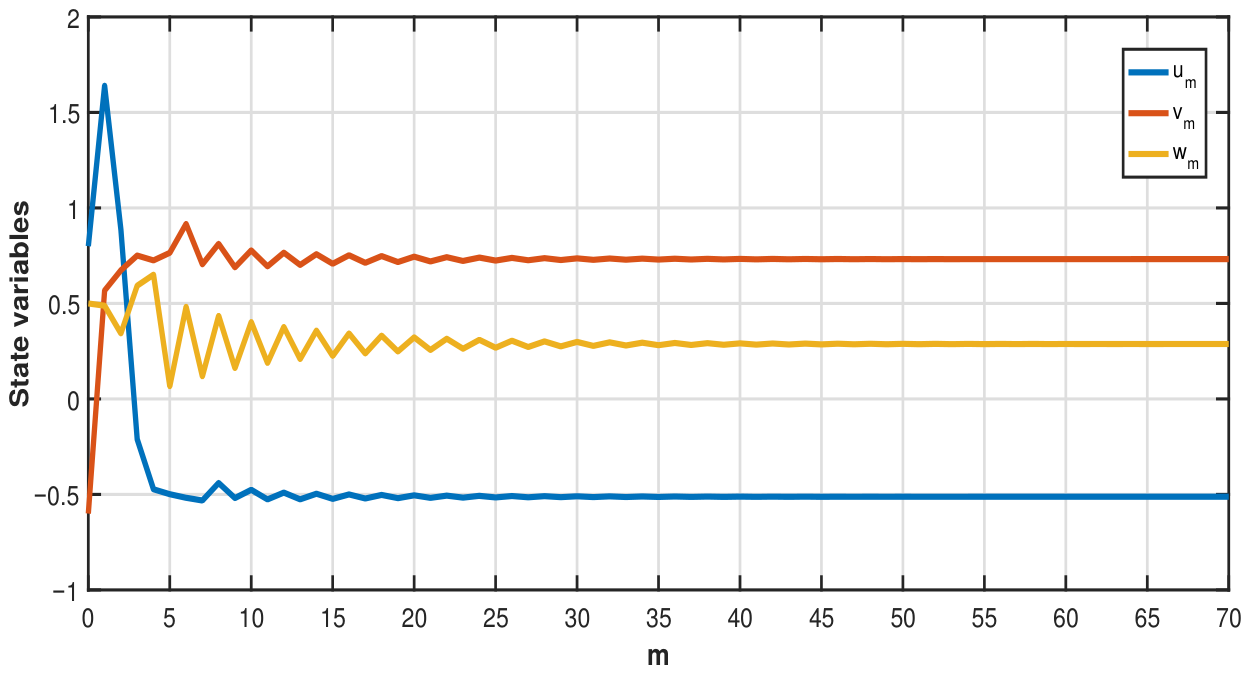
Figure 1 illustrates the graphical behavior of the sequences ( u m ) , ( v m ) , and ( w m ) .
Figure 1 demonstrates that the system, starting from distinct initial conditions, rapidly evolves toward a quasi-periodic regime, in which the sequences exhibit regular rises and falls while preserving their relative ordering. This relative stability reflects the influence of the chosen coefficients, which attenuate the system’s sensitivity to small perturbations and ensure moderate dynamical behavior. Such behavior can be regarded as a reference scenario for understanding the interaction among variables when the coefficients take small values.
Example 2. 
Consider the system (1) with the following set of parameter values:
a 1 = 0.70 , b 1 = 0.20 , c 1 = 0.05 , a 2 = 0.50 , b 2 = 0.25 , c 2 = 0.10 , a 3 = 0.60 , b 3 = 0.15 , c 3 = 0.20 .
The initial conditions are chosen as:
u 0 = 0.80 , v 0 = 0.40 , w 0 = 0.60 , u 1 = 0.30 , v 1 = 0.25 , w 1 = 0.15 .
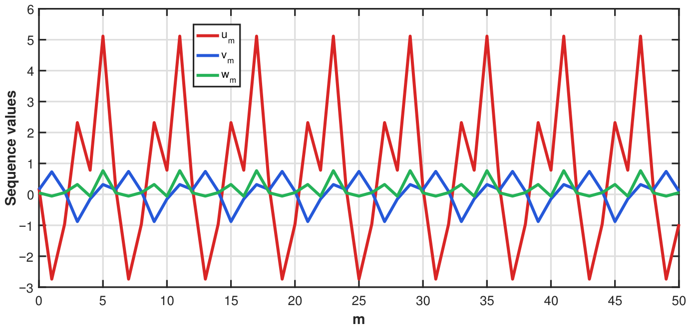
Figure 2 illustrates the graphical behavior of the sequences ( u m ) , ( v m ) , and ( w m ) .
Figure 2 illustrates a more intricate dynamical regime. In this case, the curve corresponding to u m exhibits pronounced initial jumps, whereas v m and w m respond more gradually, with temporary intersections occurring during the transient phase. This behavior reflects the influence of the negative coefficient b 1 = 0.20 , which enhances asymmetry in the interactions among the variables and introduces a higher level of dynamical irregularity, leading to larger fluctuations in the sequences. This phenomenon can be interpreted as an asymmetric perturbation of the system’s equilibrium, resulting in transient dynamical variations.
Example 3. 
Consider the system (1) with the following set of parameter values:
a 1 = 0.90 , b 1 = 0.30 , c 1 = 0.20 , a 2 = 0.90 , b 2 = 0.30 , c 2 = 0.20 , a 3 = 0.90 , b 3 = 0.30 , c 3 = 0.20 .
The initial conditions are chosen as:
u 0 = 0.50 , v 0 = 0.70 , w 0 = 0.20 , u 1 = 0.10 , v 1 = 0.30 , w 1 = 0.40 .
Figure 3 illustrates the graphical behavior of the sequences ( u m ) , ( v m ) , and ( w m ) .
In Figure 3, a high degree of symmetry is observed among the three curves, as the sequences evolve in nearly identical trajectories, often moving in parallel and converging. This behavior reflects the properties of a symmetric interaction structure and confirms that symmetry in the interaction parameters promotes uniform behavior within diversity, thereby enhancing predictability and facilitating the stability analysis of the system.
Example 4. 
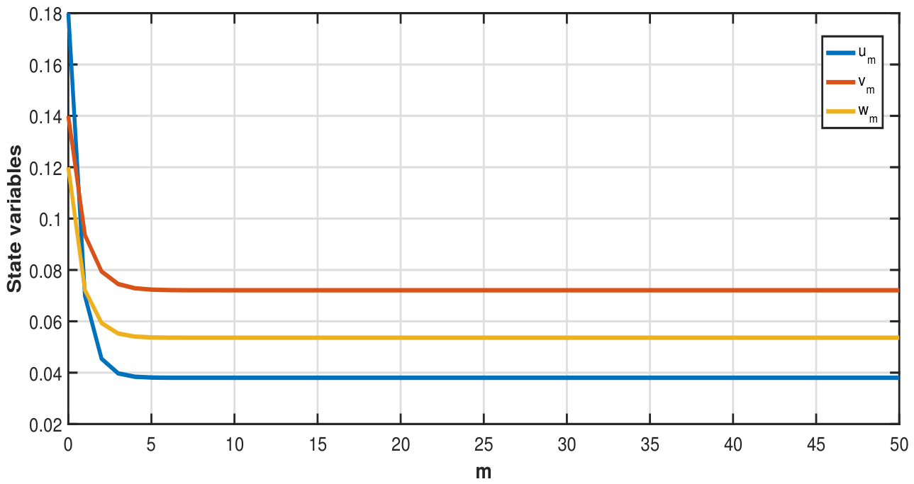
Consider the system (1) with the following set of parameter values:
a 1 = 0.15 , b 1 = 0.30 , c 1 = 0.05 , a 2 = 0.12 , b 2 = 0.25 , c 2 = 0.04 , a 3 = 0.10 , b 3 = 0.20 , c 3 = 0.03 .
The initial conditions are chosen as:
u 0 = 0.20 , v 0 = 0.15 , w 0 = 0.10 , u 1 = 0.18 , v 1 = 0.14 , w 1 = 0.12 .
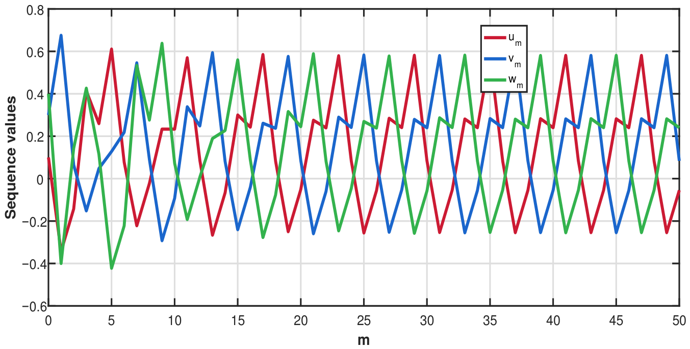
Figure 4 illustrates the graphical behavior of the sequences ( u m ) , ( v m ) , and ( w m ) .
Figure 4 depicts a comparatively “quiet” dynamical regime, in which the sequences exhibit a gradual stabilization without sharp fluctuations. The trajectories evolve smoothly and tend toward a stable pattern, reflecting the influence of small positive parameters. These parameters induce a mild stabilizing effect, leading to slow and controlled temporal variations. This behavior illustrates how stable dynamics can emerge in interconnected systems with relatively weak interactions.
Example 5. 
Consider the system (1) with the following set of parameter values:
a 1 = 0.60 , b 1 = 0.35 , c 1 = 0.35 , a 2 = 0.55 , b 2 = 0.60 , c 2 = 0.54 , a 3 = 0.65 , b 3 = 0.55 , c 3 = 0.43 .
The initial conditions are chosen as:
u 0 = 1.20 , v 0 = 0.90 , w 0 = 0.70 , u 1 = 0.80 , v 1 = 0.60 , w 1 = 0.50 .
Figure 5 illustrates the graphical behavior of the sequences ( u m ) , ( v m ) , and ( w m ) .
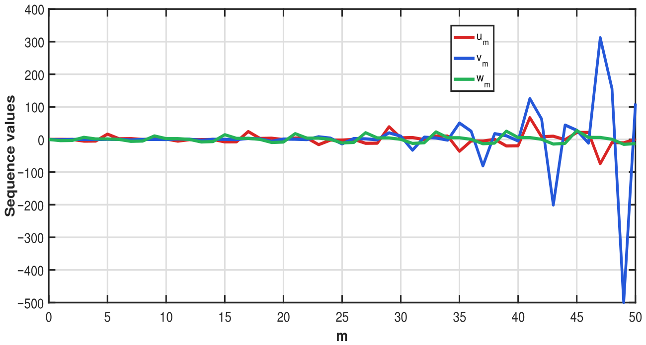
Figure 5 illustrates a highly complex dynamical regime characterized by abrupt jumps in the curves, reflecting the influence of large negative coefficients and strongly varying signals, which lead to highly volatile patterns and persistent dynamical complexity. Subsequently, the system gradually transitions toward a more stable behavior.

3. Conclusions

In this paper, we present and analyze a novel three-dimensional nonlinear system of second-order rational difference equations with periodic interactions. By employing appropriate transformations and identifying auxiliary sequences, we reduce the nonlinear system to a sixth-order periodic difference equation, enabling the derivation of explicit closed-form solutions. The system is rigorously validated under standard assumptions on the initial values and interaction coefficients, ensuring that the denominators remain nonzero within the fractional domain. Numerical examples demonstrate the richness of the system’s dynamics, highlighting oscillatory behavior, convergence, and the complex interrelationships among the sequences. This study not only generalizes previous results related to one- and two-dimensional systems but also provides a systematic methodological framework for the explicit solution of multidimensional nonlinear difference equations. These results complement recent advances in fuzzy differential theory, such as the existence and singularity results for two-dimensional systems with logarithmic interactions by Almoteri and Ghezal (2025 [34]), and the global stability analysis of higher-order fuzzy differential systems by Althaghafi and Ghezal (2025 [35]), suggesting the applicability of similar methodologies to broader classes of discrete dynamical systems characterized by uncertainty or fuzziness. Several promising directions lie ahead for future research. Extending the current framework to systems with more than three interacting components, incorporating periodic or time-varying coefficients, and exploring random or fuzzy perturbations could provide a deeper understanding of complex discrete dynamics. Furthermore, investigating the interplay between solvability, stability, and bifurcation phenomena in such multidimensional environments could yield new analytical tools for modeling applications in biology, neural networks, economics, and control systems.

Author Contributions

Methodology, A.G., A.A.A.G. and H.J.A.S.; Software, H.J.A.S.; Validation, A.A.A.G.; Formal analysis, A.A.A.G. and H.J.A.S.; Writing—original draft, A.G., A.A.A.G. and H.J.A.S.; Writing—review & editing, A.G., A.A.A.G. and H.J.A.S. All authors have read and agreed to the published version of the manuscript.

Funding

This work was supported by the Deanship of Scientific Research, Vice Presidency for Graduate Studies and Scientific Research, King Faisal University, Saudi Arabia [KFU261995].

Data Availability Statement

No new data were created or analyzed in this study. Data sharing is not applicable to this article.

Conflicts of Interest

The authors declare no conflicts of interest.

References

  1. Alzeley, O. On an asymmetric multivariate stochastic difference volatility: Structure and estimation. AIMS Math. 2024, 9, 18528–18552. [Google Scholar] [CrossRef] [Scilit]
  2. Alzeley, O. Periodic asymmetric LogGARCH stochastic volatility models: Structure and application. Axioms 2026, 15, 216. [Google Scholar] [CrossRef] [Scilit]
  3. Balegh, M.; Zemmouri, I. Markov-switching threshold stochastic volatility models with regime changes. AIMS Math. 2024, 9, 3895–3910. [Google Scholar] [CrossRef] [Scilit]
  4. Alraddadi, R. The Markov-switching threshold BLGARCH model. AIMS Math. 2025, 10, 18838–18860. [Google Scholar] [CrossRef] [Scilit]
  5. Alraddadi, R. The logTG-SV model: A threshold-based volatility framework with logarithmic shocks for exchange rate dynamics. AIMS Math. 2025, 10, 19495–19511. [Google Scholar] [CrossRef] [Scilit]
  6. Attia, N. Qualitative behavior of bidimensional rational fuzzy difference equations. Abstr. Appl. Anal. 2025, 2025, 7666805. [Google Scholar] [CrossRef] [Scilit]
  7. Althagafi, H. Solving a system of nonlinear difference equations with bilinear dynamics. AIMS Math. 2024, 9, 34067–34089. [Google Scholar] [CrossRef] [Scilit]
  8. Althagafi, H.; Ghezal, A. Stability analysis of biological rhythms using three-dimensional systems of difference equations with squared terms. J. Appl. Math. Comput. 2025, 71, 3211–3232. [Google Scholar] [CrossRef] [Scilit]
  9. Althagafi, H. Dynamics of difference systems: A mathematical study with applications to neural systems. AIMS Math. 2025, 10, 2869–2890. [Google Scholar] [CrossRef] [Scilit]
  10. Abo-Zeid, R.; Cinar, C. Global behavior of the difference equation xn+1 = Axn−1/BCxnxn−2. Bol. Soc. Parana. Mat. 2013, 31, 43–49. [Google Scholar] [CrossRef] [Scilit]
  11. Elsayed, E.M. On the solutions and periodicity of some rational systems of difference equations. Bull. Math. Soc. Sci. Math. Roum. 2017, 108, 159–171. [Google Scholar] [CrossRef] [Scilit]
  12. Elsayed, E.M. Expression and behavior of the solutions of some rational recursive sequences. Math. Methods Appl. Sci. 2016, 39, 5682–5694. [Google Scholar] [CrossRef] [Scilit]
  13. El-Metwally, H.; Elsayed, E.M. Qualitative behavior of some rational difference equations. J. Comput. Anal. Appl. 2016, 20, 226–236. [Google Scholar]
  14. Elsayed, E.M.; El-Metwally, H. Global behavior and periodicity of some difference equations. J. Comput. Anal. Appl. 2015, 19, 298–309. [Google Scholar]
  15. Alofi, B.S. Qualitative dynamics of a higher-order rational difference equation system. J. Math. Comput. Sci. 2026, 41, 519–534. [Google Scholar] [CrossRef] [Scilit]
  16. Althagafi, H. Analytical study of nonlinear systems of higher-order difference equations: Solutions, stability, and numerical simulations. Mathematics 2024, 12, 1159. [Google Scholar] [CrossRef] [Scilit]
  17. Ghezal, A.; Balegh, M.; Zemmouri, I. Solutions and local stability of the Jacobsthal system of difference equations. AIMS Math. 2024, 9, 3576–3591. [Google Scholar] [CrossRef] [Scilit]
  18. Elsayed, E.M.; El-Metwally, H. Stability and solutions for rational recursive sequence of order three. J. Comput. Anal. Appl. 2014, 17, 305. [Google Scholar]
  19. Gümüş, M. Global asymptotic behavior of a discrete system of difference equations with delays. Filomat 2023, 37, 251–264. [Google Scholar] [CrossRef] [Scilit]
  20. Gümüş, M.; Abo-Zeid, R. Global behavior of a rational second order difference equation. J. Appl. Math. Comput. 2020, 62, 119–133. [Google Scholar] [CrossRef] [Scilit]
  21. Al Salman, H.J. Closed-form solutions of systems of nonlinear difference equations and their connections to generalized Fibonacci numbers and related sequences. AIMS Math. 2025, 10, 25307–25328. [Google Scholar] [CrossRef] [Scilit]
  22. Al Ghafli, A.A. Closed-form solutions of a nonlinear bidimensional difference system via generalized Fibonacci sequences. AIMS Math. 2025, 10, 26545–26567. [Google Scholar] [CrossRef] [Scilit]
  23. Almoteri, Y. Solvability of three-dimensional nonlinear difference systems via transformations and generalized Fibonacci recursions. Mathematics 2025, 13, 3904. [Google Scholar] [CrossRef] [Scilit]
  24. Attia, N. Global stability and co-balancing numbers in a system of rational difference equations. Electron. Res. Arch. 2024, 32, 2137–2159. [Google Scholar] [CrossRef] [Scilit]
  25. Oğul, B.; Simşek, D. Dynamical behavior of one rational fifth-order difference equation. Carpathian Math. Publ. 2023, 15, 43–51. [Google Scholar] [CrossRef] [Scilit]
  26. Zhang, Y.; Yang, X.; Megson, G.M.; Evans, D.J. On the system of rational difference equations. Appl. Math. Comp. 2006, 176, 403–408. [Google Scholar] [CrossRef] [Scilit]
  27. Zhang, Q.; Yang, L.; Liu, J. Dynamics of a system of rational third order difference equation. Adv. Differ. Equ. 2012, 2012, 136. [Google Scholar] [CrossRef] [Scilit]
  28. Kara, M. Investigation of the global dynamics of two exponential-form difference equations systems. Electron. Res. Arch. 2023, 31, 6697–6724. [Google Scholar] [CrossRef] [Scilit]
  29. Elabbasy, E.; Elmatwally, H.; Elsayed, E. Qualitative behavior of higher order difference equation. Soochow J. Math. 2007, 33, 861–873. [Google Scholar]
  30. Haddad, N.; Touafek, N.; Rabago, J. Well-defined solutions of a system of difference equations. J. Appl. Math. Comput. 2018, 56, 439–458. [Google Scholar] [CrossRef] [Scilit]
  31. Yazlik, Y.; Kara, M. On a solvable system of difference equations of higher order with periodic coefficients. Commun. Fac. Sci. Univ. 2019, 68, 1675–1693. [Google Scholar] [CrossRef] [Scilit]
  32. Touafek, N.; AL-Juaid, J.G. On a second-order system of difference equations: Expressions and behavior of the solutions. AIMS Math. 2025, 10, 28077–28099. [Google Scholar] [CrossRef] [Scilit]
  33. Elaydi, S. An Introduction to Difference Equations; Springer: New York, NY, USA, 2005. [Google Scholar] [CrossRef] [Scilit]
  34. Almoteri, Y. On the existence and uniqueness of two-dimensional nonlinear fuzzy difference equations with logarithmic interactions. Mathematics 2025, 13, 3532. [Google Scholar] [CrossRef] [Scilit]
  35. Althagafi, H.; Ghezal, A. Higher-Order Fuzzy Difference Equations: Existence, Stability, and Illustrative Numerical Examples. Mathematics 2026, 14, 1051. [Google Scholar] [CrossRef] [Scilit]
Figure 1. Time evolution of the sequences ( u m ) , ( v m ) , and ( w m ) of system (1).
Mathematics 14 01396 g001
Figure 2. Time evolution of the sequences ( u m ) , ( v m ) , and ( w m ) of system (1).
Mathematics 14 01396 g002
Figure 3. Time evolution of the sequences ( u m ) , ( v m ) , and ( w m ) of system (1).
Mathematics 14 01396 g003
Figure 4. Time evolution of the sequences ( u m ) , ( v m ) , and ( w m ) of system (1).
Mathematics 14 01396 g004
Figure 5. Time evolution of the sequences ( u m ) , ( v m ) , and ( w m ) of system (1).
Mathematics 14 01396 g005
Disclaimer/Publisher’s Note: The statements, opinions and data contained in all publications are solely those of the individual author(s) and contributor(s) and not of MDPI and/or the editor(s). MDPI and/or the editor(s) disclaim responsibility for any injury to people or property resulting from any ideas, methods, instructions or products referred to in the content.