1. Introduction
The classical Ostrowski inequality, established by Ostrowski in [
1], provides an upper bound for the deviation of a differentiable function from its integral mean. More precisely, if
is continuous on
and differentiable on
with
, then for any
one has
Due to its relevance in numerical integration and error estimation, this inequality has been extended in several directions. Cerone and Dragomir [
2,
3] obtained generalizations for
n-times differentiable mappings. Liu [
4] and Alomari [
5] studied companion inequalities and applications. Further refinements under convexity assumptions, including
s-convexity, were investigated by Alomari et al. [
6] and Set et al. [
7].
The theory of time scales, introduced by Hilger and developed by Bohner and Peterson [
8], provides a unified framework for continuous and discrete analysis. Ostrowski-type inequalities on time scales were first obtained by Bohner and Matthews [
9], and further extended by Karpuz and Özkan [
10], Tuna and Daghan [
11], and Liu et al. [
12,
13,
14] who considered weighted and multi-point versions.
Additional structural improvements were studied by Sarikaya [
15], who introduced weighted Ostrowski and Čebyšev type inequalities on time scales, and further refined in [
16]. Generalized Ostrowski–Grüss inequalities were recently studied by Farid et al. [
17], and related
k-point generalizations were considered by Nwaeze et al. [
18] and Khan et al. [
19]. Cerone and Dragomir [
2] also discussed inequalities for functions satisfying convexity-type conditions. Earlier companion results of Alomari [
5] and Liu [
4] remain fundamental for understanding these developments.
Based on these results, this paper presents new two-sided Ostrowski-type inequalities on arbitrary time scales. The main assumption is that the delta derivative satisfies
where
m and
M are delta integrable functions. With additional monotonicity conditions on these limiting functions, it leads to sharper and more computable estimates. The results are particularly applicable to uniform time scales such as
and quantum time scales such as
.
The main novelty of the present paper lies in replacing the classical constant derivative bounds by variable monotone functions on arbitrary time scales. As a consequence, the obtained inequalities yield locally adaptive error estimates that reflect the graininess structure of the underlying time scale.
2. Preliminaries and Basic Definitions
For a comprehensive introduction to time scales calculus, we refer to Bohner and Peterson [
8]. A time scale
is a nonempty closed subset of
. The forward and backward jump operators
are defined by
The forward graininess function is
2.1. Delta Differentiation and Integration
A function
is said to be delta differentiable at
if there exists a number
such that, for every
, there exists a neighborhood
U of
satisfying
for all
.
The fundamental identity
holds whenever
f is delta differentiable at
.
The Cauchy delta integral is defined by
whenever
on
.
In particular:
2.2. Integration by Parts on Time Scales
If
f and
g are delta differentiable on
, then
or equivalently,
2.3. Basic Properties of the Delta Derivative
For delta differentiable functions and constants :
- 1.
.
- 2.
.
- 3.
In particular, on
,
- 4.
On
, for
,
3. Two-Sided Ostrowski-Type Inequalities on Time Scales
In this section, we develop a unified approach to Ostrowski-type inequalities on arbitrary time scales. The results are obtained by estimating the delta derivative of the basis function through appropriate integrable comparison functions. This approach provides sharp error bounds for the Ostrowski functional in a general time scale setting and will allow us to recover various continuous, discrete, and quantum versions known as special cases.
Theorem 1.
Let be a time scale and let be delta differentiable on . Assume that is delta integrable on and that there exist delta integrable functions such thatThen, for every , the following two-sided Ostrowski-type inequality holds: Proof. Fix
. For any
, by the Fundamental Theorem of Calculus on time scales,
Integrating both sides with respect to
over
, we obtain
The left-hand side simplifies to
Since
is delta integrable, we may change the order of delta integration. Splitting the region according to
and
, we obtain
Using the identity valid on any time scale,
we have
Hence,
Dividing by
, we obtain the identity
Since
and the weights
and
are nonnegative on their respective intervals, we obtain
and
Adding these inequalities and multiplying by
yields (
2). □
The bounds obtained in Theorem 1 can be further improved by introducing additional structural assumptions to the limiting functions. In particular, monotonicity leads to sharper and more explicit estimates.
Proposition 1.
Let be a time scale and let with . Assume that is delta differentiable on and that is delta integrable on . Suppose that there exist delta integrable functions such thatIf m and M are monotone on , then the bounds in Theorem 1 admit the estimates Proof. From Theorem 1 we have
Assume that
m is monotone increasing on
. Then
Using
and the positivity of the weights
and
, we obtain
Substituting these estimates into the above identity yields the lower bound. For the upper bound, assume that
M is monotone increasing on
. Then
Using
and the positivity of the weights
and
, we obtain the corresponding upper estimate, which yields the stated bound. □
Remark 1.
It is worth noting that the termsnaturally depend on the graininess function of the time scale. Indeed, on any time scale the identityholds. Therefore, the lower and upper bounds obtained in Proposition 1 inherently incorporate the local structure of the time scale through the graininess function. This provides a refined error estimate compared with the classical continuous case where . Remark 2.
The bounds obtained in Proposition 1 are sharp for the class of functions whose delta derivatives are monotone. Indeed, if itself is a monotone function on , we may chooseSubstituting this choice into the bounds of Proposition 1 reduces the inequalities to equalities and exactly reproduces the error functionalHence the obtained bounds are best possible for this class of functions. Remark 3.
The estimates obtained in Theorem 1 and Proposition 1 are closely related to recent results in the literature. In particular, results similar in spirit were considered in [16], where inequalities on time scales were derived under derivative bounds given by constants. The present results differ from [16] in two main aspects. First, the bounds for are given by monotone functions m and M rather than constants, which allows a more flexible description of the behavior of the derivative. Second, the obtained estimates explicitly reflect the structure of the time scale through the delta integralswhose values depend on the graininess function . Consequently, the bounds obtained here may provide sharper estimates, especially on nonuniform or discrete time scales where the graininess function varies.
Comparison with Classical Ostrowski-Type Inequalities
Table 1 highlights the main differences between the classical Ostrowski inequality, its time scale extension, and the result obtained in Proposition 1.
The comparison shows that the present results provide more flexible bounds since the derivative constraints are allowed to vary along the time scale.
Example 1.
Let and consider the function on . ThenTakingwhich are monotone functions on , the bounds obtained in Proposition 1 reduce to equalities. For we computeThis example illustrates that the bounds in Proposition 1 are exact for functions with monotone derivatives. Example 2.
Let with step size and consider on . The delta derivative becomesThus the derivative bounds can be chosen asApplying Proposition 1 yields bounds that explicitly depend on the graininess h of the time scale. Example 3.
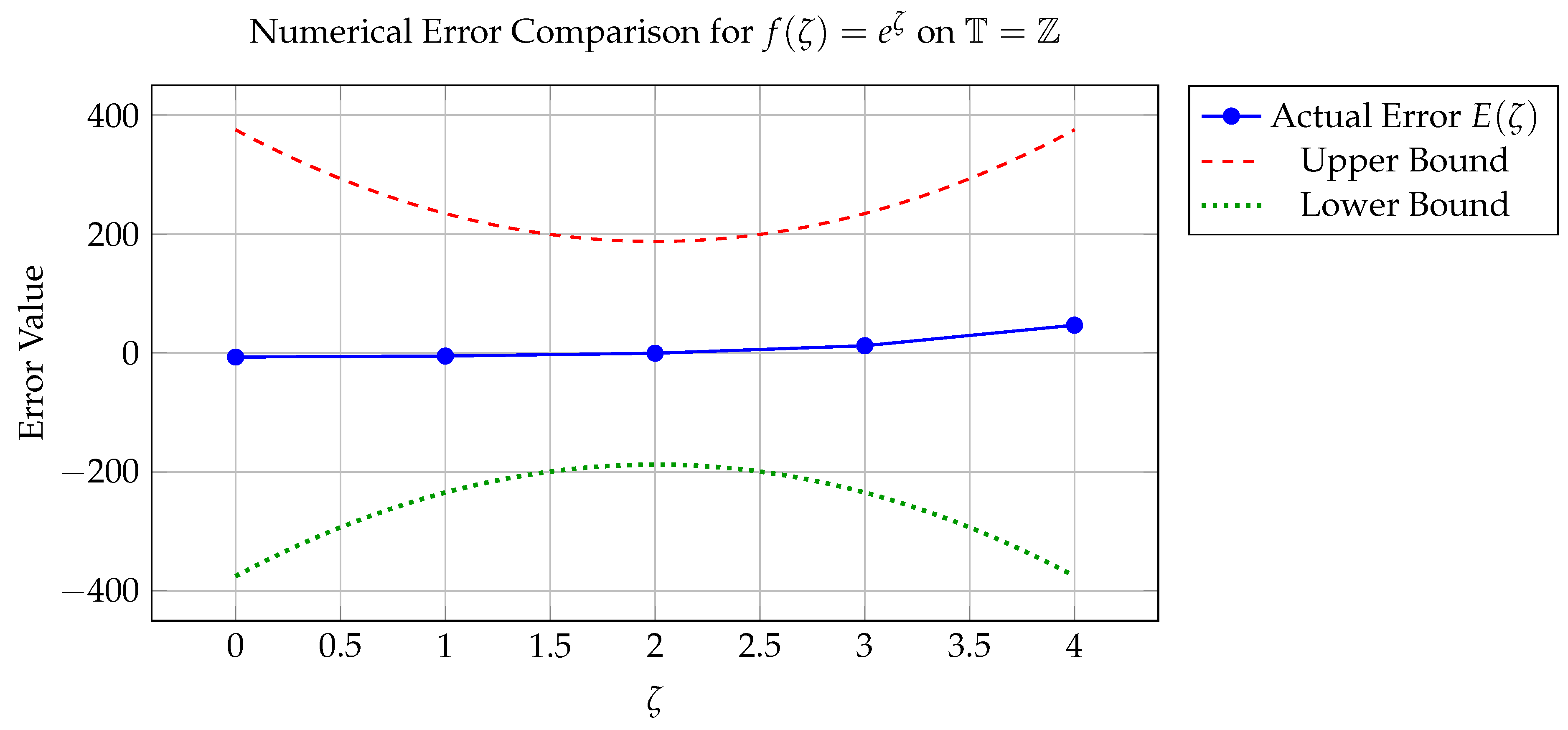
Consider the exponential function on the time scale or . The delta derivative is given byApplying the two-sided Ostrowski-type inequality from Proposition 1, we haveFor the interval and , the delta derivative values areand the actual error is bounded betweenThe numerical comparison between the actual error and the theoretical bounds can be plotted as in Figure 1. 4. Error Analysis
Now, let us show how Theorem 1 is reduced to classical discrete Ostrowski inequalities by considering certain choices of time scales as follows:
Corollary 1.
Let with , and let be a real sequence. Assume that there exist real constants L and U such thatThen, for any , the following inequality holds: Proof. This result follows as a direct specialization of Theorem 1 to the time scale .
On the integer time scale, the delta derivative reduces to the forward difference operator,
and the delta integral becomes a finite sum,
Substituting these identities into inequality (
2) of Theorem 1 yields
Under the additional assumption that the bounds are constant, namely
and
for all
k, the weighted sums can be evaluated explicitly using standard formulas for arithmetic series:
and
Substituting these expressions into the previous inequality immediately yields (
3), which completes the proof. □
Remark 4.
If is even and is the midpoint of the interval, then inequality (3) reduces towhich represents the discrete analogue of the classical Ostrowski inequality for differentiable functions. Corollary 2.
Let and let be the quantum time scale. Assume that with , and let be continuous on and delta differentiable on . Suppose that is delta integrable and that there exist delta integrable functions such thatThen, for every , the following quantum Ostrowski-type inequality holds: Proof. The result follows directly from Theorem 1 by choosing the time scale .
On the quantum time scale, the delta derivative is
and the delta integral reduces to the weighted sum
Applying these representations to the integrals appearing in (
2), we obtain
which completes the proof. □
Remark 5.
Assume that the bounds of the delta derivative are constants, that is, and with . Then inequality (4) yields the explicit quantum Ostrowski-type estimateOn the quantum time scale , the delta integrals admit the explicit representationsMoreover, as , the quantum delta derivative and delta integral converge to the classical derivative and the Riemann integral, and the above estimate reduces to the classical Ostrowski inequality on real intervals. Corollary 3.
Let and let . Assume that with , and let . Suppose that there exist functions such that Then, for every , the following discrete Ostrowski-type inequality holds: Remark 6.
This corollary follows from Theorem 1 by taking the uniform time scale . Let with . On this time scale, the forward jump operator satisfies , the graininess function is constant , and the delta derivative reduces toMoreover, for any function , the delta integral over becomesTherefore, inequality (5) represents the discrete version of Theorem 1 on the uniform lattice . In particular, when , it reduces to the classical Ostrowski-type inequality for integer sequences. Corollary 4.
Let and let . Assume that with , and let . Suppose that the forward differences satisfy the constant boundsThen, for any , the following explicit Ostrowski-type inequality holds: Proof. From Corollary 3, setting
and
, we obtain
where
Using the classical Gauss summation formula
we compute
and
Adding these expressions yields
Multiplying by
completes the proof. □
Proposition 2. Let be a time scale and let with . Assume that is delta differentiable on and thatwhere m and M are delta integrable and monotone functions on . Then, for any , the following estimates hold. - (i)
If m is increasing on , then - (ii)
If m is decreasing on , then Analogous inequalities hold for M with the inequality signs reversed where appropriate.
Proof. We prove part (i); part (ii) follows analogously by reversing the inequalities.
Assume that
m is increasing on
. Then, for all
, we have
. Since
on this interval, it follows that
Integrating both sides with respect to the delta integral yields
Similarly, for
, monotonicity of
m implies
, and since
, we obtain
Adding the two inequalities completes the proof of part (i). □
Remark 7.
If , then the delta integral coincides with the classical Riemann integral and the identitieshold exactly. In this case, Proposition 2 reduces to the classical monotone bounds used in Ostrowski-type inequalities. For general time scales, the integralsdepend on the graininess function and are, therefore, left in integral form. Remark 8.
Proposition 2 significantly enhances the applicability of the main theorem on time scales. In discrete settings, such as or , the error bounds can be evaluated by using only finitely many terms of a sequence, avoiding the explicit computation of delta integrals. In quantum calculus, where the q-integral may become technically involved, the monotonicity of the bounding functions allows one to estimate the bounds using only endpoint values. This feature makes the result particularly effective for numerical and computational purposes.
Example 4.
Let with , and consider the interval for some . Let , so thatClearly, is increasing on . SetFor with , Proposition 2 yieldsSinceand the bound is obtained explicitly in terms of finite sums, without any approximation. Example 5.
Let with , and consider the interval , where are integers. LetThen the delta derivative on is given byHence is increasing on . DefineFor with , Theorem 1 givesSince is increasing on , Proposition 2(i) impliesConsequently, we obtain the estimatewhich provides a sharper Ostrowski-type bound expressed only in terms of the endpoint values and . In this section, we analyze the deviation between the function value and its delta integral mean over the interval . Throughout, we follow the notation of Theorem 1.
Define the error functional by
4.1. Error Bound Under Derivative Constraints
Assume that
as in Theorem 1. If
with constants
, then Theorem 1 yields
4.2. Minimizing the Error Bound
Set
In the continuous case
,
which is minimized at
For uniform discrete time scales
, the minimum is attained at a grid point closest to
.
4.3. Endpoint Behavior on Uniform Time Scales
For
,
and, therefore,
5. Numerical Illustration of the Error Bound
In this section, we illustrate the sharpness of Theorem 1 on the uniform discrete time scale . The purpose is to compare the actual error with the theoretical bound.
6. Conclusions
In this paper, we established two-sided Ostrowski-type inequalities on arbitrary time scales by assuming upper and lower bounds for the delta derivative of the function. The obtained inequalities provide explicit estimates for the deviation and include, as particular cases, the classical continuous, uniform discrete, and quantum settings.
Furthermore, the established results provide a rigorous “safety corridor” for error estimation in the numerical analysis of dynamic equations on time scales. In practical scenarios such as population dynamics or control theory, where growth rates or parameters often vary monotonically, our bounds offer a reliable tool to determine the maximum possible deviation from average behavior without requiring an exact solution to the dynamic equation. This connection between abstract time scale theory and applied dynamic systems ensures the robustness of numerical simulations across non-uniform time domains.
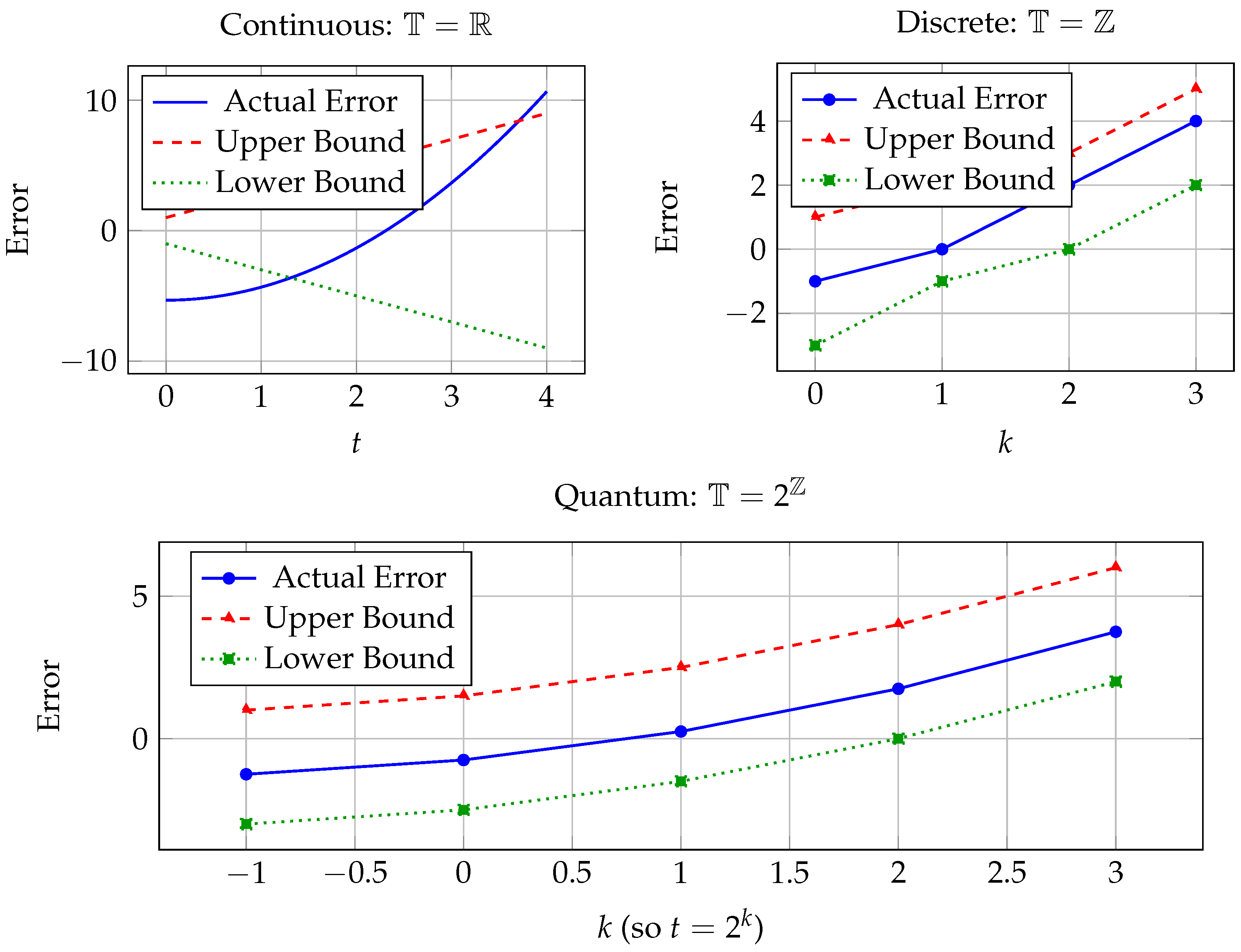
Under additional monotonicity assumptions regarding the limiting functions, improved integral estimates were obtained that remained fully consistent with the structure of the underlying time scale. These improvements are particularly important when the granularity function is not constant, since the error limit then clearly depends on the time scale geometry. Numerical samples on uniform discrete and quantum time scales validate the theoretical predictions. The approach developed here can be extended to weighted Ostrowski-type inequalities or inequalities involving higher-order delta derivatives.
Author Contributions
Conceptualization, R.T.A.; Methodology, R.T.A., N.H.A. and M.Z.S.; Software, N.H.A. and M.Z.S.; Validation, R.T.A., N.H.A. and M.Z.S.; Formal analysis, R.T.A., N.H.A. and M.Z.S.; Investigation, R.T.A., N.H.A. and M.Z.S.; Resources, R.T.A., N.H.A. and M.Z.S.; Data curation, R.T.A., N.H.A. and M.Z.S.; Writing—original draft, R.T.A., N.H.A. and M.Z.S.; Writing—review & editing, R.T.A., N.H.A. and M.Z.S.; Visualization, R.T.A. and N.H.A.; Supervision, R.T.A.; Funding acquisition, R.T.A. and N.H.A. All authors contributed equally to the writing of this paper. All authors have read and agreed to the published version of the manuscript.
Funding
This work was supported and funded by the Deanship of Scientific Research at Imam Mohammad Ibn Saud Islamic University (IMSIU) (grant number IMSIU-DDRSP2602).
Data Availability Statement
No new data were created or analyzed in this study.
Conflicts of Interest
The authors declare no conflicts of interest.
References
- Ostrowski, A. Über die Absolutabweichung einer differentiierbaren Funktion von ihrem Integralmittelwert. Comment. Math. Helv. 1937, 10, 226–227. [Google Scholar] [CrossRef]
- Cerone, P.; Dragomir, S.S. Ostrowski Type Inequalities for Functions Whose Derivatives Satisfy Certain Convexity Assumptions. Demonstr. Math. 2004, 37, 299–308. [Google Scholar] [CrossRef]
- Cerone, P.; Dragomir, S.S.; Roumeliotis, J. Some Ostrowski type inequalities for n-time differentiable mappings and applications. Demonstr. Math. 1999, 32, 697–712. [Google Scholar] [CrossRef]
- Liu, Z. Some Ostrowski type inequalities and applications. Vietnam J. Math. 2009, 37, 15–22. [Google Scholar]
- Alomari, M.W. A companion of Ostrowski’s inequality for mappings whose first derivatives are bounded and applications in numerical integration. Kragujev. J. Math. 2012, 36, 77–82. [Google Scholar]
- Alomari, M.; Darus, M.; Dragomir, S.S.; Cerone, P. Ostrowski Type Inequalities for Functions Whose Derivatives Are s-Convex in the Second Sense. Appl. Math. Lett. 2010, 23, 1071–1076. [Google Scholar] [CrossRef]
- Set, E.; Özdemir, E.M.; Sarikaya, M.Z. New inequalities of Ostrowski’s type for s-convex functions in the second sense with applications. Facta Univ.-Ser. Math. Informatics 2012, 27, 67–82. [Google Scholar]
- Bohner, M.; Peterson, A.C. Dynamic Equations on Time Scales: An Introduction with Applications; Birkhaäuser: Boston, MA, USA, 2001. [Google Scholar]
- Bohner, M.; Matthews, T. Ostrowski Inequalities on Time Scales. J. Inequal. Pure Appl. Math. 2008, 9, 1–8. [Google Scholar]
- Karpuz, B.; Özkan, U.M. Generalized Ostrowski’s Inequality on Time Scales. J. Inequal. Pure Appl. Math. 2008, 9, 1–7. [Google Scholar]
- Tuna, A.; Daghan, D. Generalization of Ostrowski and Ostrowski–Grüss Type Inequalities on Time Scales. Comput. Math. Appl. 2010, 60, 803–811. [Google Scholar] [CrossRef]
- Liu, W.; Tuna, A.; Jiang, Y. On weighted Ostrowski type, trapezoid type, Grüss type and Ostrowski-Grüss like inequalities on time scales. Appl. Anal. 2014, 93, 551–571. [Google Scholar] [CrossRef]
- Liu, W.; Ngô, Q.A. A generalization of Ostrowski inequality on time scales for k points. Appl. Math. Comput. 2008, 203, 754–760. [Google Scholar] [CrossRef]
- Liu, W. An Ostrowski-Grüss type inequality on time scales. Comput. Math. Appl. 2009, 58, 1207–1210. [Google Scholar] [CrossRef]
- Sarikaya, M.Z. New weighted Ostrowski and Čebyšev type inequalities on time scales. Comput. Math. Appl. 2010, 60, 1510–1514. [Google Scholar] [CrossRef]
- Sarikaya, M.Z.; Budak, H. Weighted Čebyšev- and Ostrowski-type inequalities on time scales. Int. Geom. Methods Mod. Phys. 2025, 22, 2450291. [Google Scholar] [CrossRef]
- Farid, G.; Mehmood, S.; Younis, B.A.; Ahamd, H.U.M.; Egami, R.H.; Adam, A.M.I. Generalized Ostrowski and Ostrowski-Grüss type inequalities. Rend. Del Circ. Mat. Di Palermo 2024, 73, 3241–3251. [Google Scholar] [CrossRef]
- Nwaeze, E.R.; Kermausuor, S.; Tameru, A.M. New time scale generalizations of the Ostrowski-Grüss type inequality for k points. J. Inequal. Appl. 2017, 2017, 245. [Google Scholar] [CrossRef] [PubMed]
- Khan, A.R.; Mehmood, F.; Shaikh, M.A. Generalization of the Ostrowski inequalities on time scales. Vladikavkaz Math. J. 2023, 25, 98–110. [Google Scholar] [CrossRef]
| Disclaimer/Publisher’s Note: The statements, opinions and data contained in all publications are solely those of the individual author(s) and contributor(s) and not of MDPI and/or the editor(s). MDPI and/or the editor(s) disclaim responsibility for any injury to people or property resulting from any ideas, methods, instructions or products referred to in the content. |