Looking into the i of the Storm: An Overview of Mid-1880s Contingency Table Indices for Studying Tornado Data

Abstract

One of the first serious attempts to study the indices that assess the association between the variables of a 2 × 2 contingency table was undertaken in the mid-1880s. Central to this study is the 1884 tornado observation/prediction data collected by Seargent John Park Finley (1854–1943), while working for the US Army Signal Service, and the controversial index he proposed to evaluate the success of his tornado predictions, which he denoted i. Subsequent improvements to Finley’s index were proposed, all of which pre-date the development of association measures made by pioneers such as Sir Francis Galton and Karl Pearson. This paper discusses Finley’s data, his index i, and the improvements made to this index. We also give historical context to Finley and his successors and their place in the early development of contingency table analysis.

1. Introduction

The contingency table remains one of the most ubiquitous ways of displaying data, especially data of a categorical nature; these categories may exist as “natural” distinctions of traits or characteristics or arise by converting numerical data so that each datum falls within an interval scale. Altham and Ferrie [1] (p. 3) said of the contingency table:

“Few tools are as useful to the social historian as the humble contingency table. In a matter of a few columns and rows, it can summarize information on an entire population and reveal striking patterns of association between characteristics. And it can make these relationships comprehensible even to readers who lack substantial statistical sophistication.”

Stigler [2] provides an excellent historical account of the analysis of the contingency table. He does so by first discussing the contributions made by Sir Francis Galton (1822–1911) and then talks of those by Galton’s protégé Karl Pearson (1857–1936), and of George Udny Yule (1871–1951) and Maurice Bartlett (1910–2002). Stigler [2] also points to the earlier contributions of Ireneé-Jules Bienaymé (1796–1878), Mikhail Vasilyevich Ostrogradsky (1801–1862), and Carl von Liebermeister (1833–1901) as key early contributors to the analysis of the 2 × 2 contingency table. Agresti [3] (Chapter 17) provides a historical tour of categorical data analysis by discussing the contributions made by Pearson and Yule but also includes the impact made by Sir Ronald A. Fisher (1890–1962). Therefore, it should be no surprise that the story of the formal, and rigorous, methods used to analyze the contingency table often begins in 1892. It was this year that Galton [4] analyzed the fingerprints of 105 pairs of fraternal twin brothers. His data and their analysis are important not just because of the impact they had on contingency table analysis (which I talk more about in Section 3.4) but also because Galton’s study was aided by his 1889 description of correlation [5]. However, it is the development of Pearson’s chi-squared statistic [6] that is often viewed as the mathematical origin of modern contingency table analysis. Lancaster [7] also provides an excellent discussion of the pre-history (that is, prior to Pearson [6]) of the chi-squared statistic. One that should not be neglected from any discussion on the early period of contingency table analysis is George Udny Yule. He was very much interested in examining the technical and practical implications of correlation, association, and its relationship to contingency tables [8,9]. Fienberg and Rinaldo [10] (Section 2.1) and, shortly after, Fienberg [11] (p. 173) point out that “most papers and statistical textbooks on categorical data analysis trace the history” back only as far as to the contributions of Pearson and Yule. The legacy left by Galton, Pearson, and Yule, and their contributions to contingency table/categorical data analysis, are deservingly still being felt amongst the statistical and her allied communities. However, the seeds of several of their ideas had been sown at least a decade earlier and in a very different part of the world. It is these seeds that shall be the focus of this paper. I begin by providing some background on those who first planted these seeds.

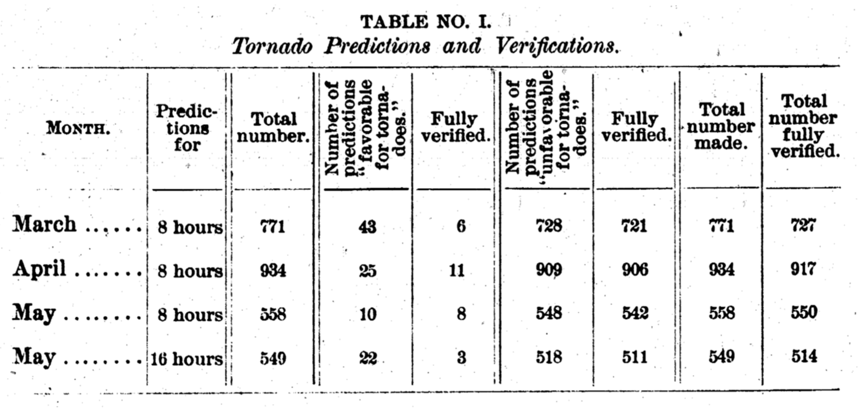
The seeds of modern-day contingency table analysis must acknowledge the contributions made by a quartet of American meteorologists/scientists in the mid-1880s who developed a range of indices to help verify the accuracy of tornado predictions in central USA. The first of these indices was put forward by Seargent John Park Finley (1854–1943) in 1884 who, while working for the US Army Signal Service, accompanied his index with four data sets that were formed by studying the number of successful and unsuccessful tornado predictions he made as well as the number of tornadoes that occurred and did not occur [12]. It must be pointed out at the outset that Finley’s index is fundamentally flawed (something I discuss at length throughout this paper); however, its importance stems primarily from the attention that quickly followed which focused on improving the quality and interpretability of his index. The contributors of these developments are very rarely, if ever, given full recognition outside of the meteorological communities, and there are only a very small number of exceptions that give some recognition to their contributions in the statistics literature; Goodman and Kruskal [13] (Section 3.1), Rovine and Anderson [14], Baker and Kramer [15], and Armistead [16] serve as examples of these exceptions. Therefore, this paper will discuss Finley’s tornado data—a screenshot of this data from his 1884 paper is given by Figure 1—and the index he developed for studying this data. This paper also provides a thorough discussion of the improvements made to Finley’s index that were put forward by Grobe Karl Gilbert (1843–1918) [17], Charles Sanders Peirce (1839–1914) [18], and Myrick Hascell Doolittle (1830–1913) [19]. We shall refer to Finley, Gilbert, Peirce, and Doolittle collectively as the “US quartet” with Finley’s index and data and the subsequent attention it gained described as the “Finley affair” [20].

This paper consists of the following six sections. I start by discussing Finley’s data in Section 2 and its presentation as a 2 × 2 contingency table formed from the cross-classification of the variables Predicted and Occurrence—these being the number of tornadoes that Finley predicted or failed to predict (Predicted) and the number of tornadoes that were observed to have occurred or not occurred (Occurrence).

Table 1. Notation of a generic 2 × 2 contingency table.

	Occurrence
Prediction	Tornado	No Tornado	Total
Tornado	${\mathrm{n}}_{11}$	${\mathrm{n}}_{12}$	${\mathrm{n}}_{1•}$
No Tornado	${\mathrm{n}}_{21}$	${\mathrm{n}}_{22}$	${\mathrm{n}}_{2•}$
Total	${\mathrm{n}}_{•1}$	${\mathrm{n}}_{•2}$	$\mathrm{n}$

summarizes the notation that will be used in this paper and defines a generic 2 × 2 contingency table. The sample size and the (1, 1)’th cell frequency is denoted by $\mathrm{n}$ and ${\mathrm{n}}_{11}$, respectively, while the first and second row (and column) marginal frequencies are denoted by ${\mathrm{n}}_{1•}$ and ${\mathrm{n}}_{2•}$ (${\mathrm{n}}_{•1}$ and ${\mathrm{n}}_{•2}$), respectively. Section 2 also describes the index that Finley proposed for assessing the accuracy of his predictions.

Gilbert’s [17] improvement of Finley’s [12] index is then discussed in Section 3 as is Gilbert’s proposal of e, a quantity that is equivalent to the expected frequency of the (1, 1)’th cell under independence between the Predictions and Occurrence variables. Section 4 and Section 5 discuss the indices of Peirce [18] and Doolittle [19], respectively. It is important to point out that Murphy [20] also provides a review of the indices presented by the US quartet. Although, where this paper differs from Murphy’s [20] is that the discussions made throughout Section 2, Section 3, Section 4 and Section 5 (inclusive) provide additional perspectives and discussions on the relevance of this early work to the foundations of contingency table analysis established by Galton, Pearson, and others. This paper also discusses how these indices and their contributions fit within the contingency table literature today. Unlike much of the literature that discusses the work of our US quartet, Section 6 will provide a thorough assessment of the features of each index with special attention given to their bounds, linkages, and behavior for changes in the ${\mathrm{n}}_{11}$ cell frequency. Some final remarks will be made in Section 7.

2. Finley’s Tornado Predictions

2.1. Finley’s Data

Finley’s [12] first data set in Figure 1 comes from predictions he made of a tornado occurring (or not) and the observations recorded on 10 March 1884, across 18 districts of the USA. Finley’s data are based on the observations and predictions he made that lie east of 105° longitude with “tornado alley” being on the western limit of this region. He started his predictions during the eight-hour period that day starting at 7 a.m. (Washington time). A second set of predictions was then made at 3 p.m. for the eight-hour period ending at 11 p.m. Further predictions of whether a tornado would be observed were made in April and twice in May.

Table 2. Finley’s tornado data of April 1884.

	Occurrence
Prediction	Tornado	No Tornado	Total
Tornado	11	14	25
No Tornado	3	906	909
Total	14	920	934

shows Finley’s data based on his observations and predictions in April 1884. Note that Finley made 934 predictions of which 11 tornadoes were predicted AND observed. Of central importance to many of the discussions of this data are the 906 predictions that Finley made of a tornado not occurring AND were observed to have not occurred.

2.2. The “Index of Verification”

Based on the data in Table 2, Finley calculated his index of verification, being the probability of successfully predicting whether a tornado would be observed or not, as:

$$i_{\mathrm{F}}={\displaystyle \frac{11+906}{934}}=0.9818.$$

This index suggests that 98.18% of the forecasts that Finley made were correct, an impressively large percentage. Finley [12] denoted his index by $i$ and so this convention is followed in this paper with a small, but important, refinement; the subscript “F” has been added here to distinguish it from indices proposed by others. With a few exceptions, improvements to $i_{\mathrm{F}}$ are also denoted by $i$ in this paper with the first letter of the author’s surname appearing in the subscript.

It is worth pointing out that Finley did not perform his calculations using any form of notation. Although, based on the notation outlined in Table 1, his index is defined by:

$$i_F={\displaystyle \frac{{\mathrm{n}}_{11}+{\mathrm{n}}_{22}}{\mathrm{n}}}.$$

(1)

Repeating the calculation of Finley’s April index for the predictions and observations made in March, May (8-h observation) and May (10-h observation) produce an $i_F$ index of 0.9429, 0.9857, and 0.9519, respectively. By aggregating each of the cell frequencies of the four 2 × 2 contingency tables from the data given in Figure 1, the overall probability of Finley [12] successfully predicting whether a tornado would be observed or not is 0.9661.

3. Gilbert’s Analysis

3.1. The “Ratio of Verification” Index

Gilbert [17] argued that predicting the number of tornadoes to occur should be based not just on the “favorable” predictions that Finley made but also on his “unfavorable” predictions. This is because the final prediction should be determined by not just how successful a prediction is—like Finley did—but that it should also be determined based on how unsuccessful the prediction is. Therefore, Gilbert defined:

▪

the number of “favorable” predictions to be those that occurred and those that did not occur, being ${\mathrm{n}}_{11}$ and $\left({\mathrm{n}}_{1•}-{\mathrm{n}}_{11}\right)$ respectively. Therefore, the total number of favorable predictions is ${\mathrm{n}}_{11}+\left({\mathrm{n}}_{1•}-{\mathrm{n}}_{11}\right)={\mathrm{n}}_{1•}$.

▪

the number of “unfavorable” predictions to be the number of tornadoes that occurred but were not predicted, this quantity being ${\mathrm{n}}_{•1}-{\mathrm{n}}_{11}$.

Therefore, Gilbert’s [17] (Equation (1)) probability of successfully predicting whether a tornado would be observed or not is:

$$v={\displaystyle \frac{{\mathrm{n}}_{11}}{{\mathrm{n}}_{1•}+\left({\mathrm{n}}_{•1}-{\mathrm{n}}_{11}\right)}}$$

(2)

and he referred to this as his ratio of verification. Gilbert’s index, (2), can also be expressed alternatively, and equivalently, by:

$$v={\displaystyle \frac{{\mathrm{n}}_{11}}{\mathrm{n}-{\mathrm{n}}_{22}}}={\displaystyle \frac{{\mathrm{n}}_{11}}{{\mathrm{n}}_{11}+{\mathrm{n}}_{12}+{\mathrm{n}}_{21}}}$$

and is still being used in the meteorological community where it is referred to as the critical success index (CSI) or threat score (Schaeffer [21,22]; Hogan et al. [23]). It should be noted that after Gilbert proposed (2) it was independently derived and used across a range of other disciplines. For example, it is equivalent to the coefficient discussed by Jaccard [24] who, in 1912, studied the distribution of flora across the French/Swiss Alpine region. It is also equivalent to the similarity coefficient of Sneath [25] (p. 203) who was concerned with bacterial classification.

Interestingly, unlike Finley’s index (1), Gilbert’s index (2) does not include ${\mathrm{n}}_{22}$; even removing it from the sample size in the denominator of $v$. When describing the various indices that can be obtained from an analysis of Table 1 (at least for ecological purposes), Janson and Vegelius [26] suggest that all indices should be independent of ${\mathrm{n}}_{22}$ noting that if it is not ignored it:

“… would tend to give a high value [of the index], indicating a high degree of coexistence between very rare species, even if they are seldom found together.”

[26] (p. 371)

This is certainly the case for Finley’s results. Gilbert was also aware of this saying of Finley’s observations:

“The occurrence of tornadoes in any given one of the districts indicated by him, is highly exceptional; their non-occurrence is the rule; and this consideration is overlooked when the predictions of occurrence and non-occurrence are classed together as of equal difficulty.”

[17] (p. 166)

Therefore, calculating Gilbert’s ratio of verification, (2), for Table 2, the probability of successfully predicting whether a tornado will occur or not is:

$$v={\displaystyle \frac{11}{14+25-11}}=0.3929$$

which is very different to Finley’s index of 0.9818. Similarly, the value of $v$ for the March, May (8-h) and May (10-h) observations are 0.1200, 0.5000, and 0.1034, respectively. Aggregating the four 2 $\times$ 2 tables produces an overall ratio of verification of 0.2276. Without knowing more about the behavior of $v$ for each data set, such as its bounds, its value cannot be clearly interpreted. Therefore, in Section 6.2 and Section 6.5 discussions are made on how reasonable the indices $i_F$ and $v$ are for quantifying the successful prediction of a tornado occurring or not.

3.2. Gilbert’s Revised Index and “e”

Gilbert [17] was not completely satisfied with his $v$. He realized that one aspect of his analysis that was missing was how good the predictions were compared to whether a prediction had been made by chance. Gilbert provided a clear explanation of the ratio of what is observed to what is expected to occur by “coincidence” saying:

“It is to be observed, however, that the ratio of verification falls far short of a just measure of success in scientific forecasting, for with the same skill in inference this ratio may be larger or smaller according as the phenomena foretold are normally frequent or rare.”

[17] (p. 168)

Therefore, Gilbert adjusted (2) by noting that (keeping to his original spelling and using the notation of Table 2):

“If the forcaster were to make his ${\mathrm{n}}_{1•}$ predictions at random it is probable that a certain number, e, of predictions would fortuitously coincide with occurrences. Making his predictions by the aid of inference, the number of coincidences is n₁₁. n₁₁ − e coincidences are thus the product of his skill in inference, and n₁₁ − e may be regarded as a measure of his success in inference, in precisely the same sense in which n₁₁ has been regarded above as a measure of verification.”

[17] (p. 168)

Such a comment reflects what “G” [27] (author unknown) colorfully stated in 1884 when referring to Finley’s analysis of the March results:

“… An ignoramus in tornado studies can predict no tornadoes for a whole season and obtain an average of fully ninety-five percent. The value of the expert work must, therefore, be measured by the excess which is obtained over the man who knows nothing of the subject.”

[17] (p. 126)

The excess that “G” speaks of is exactly what Gilbert’s $e$ assesses. Gilbert [17] (Equation (2)) then defined a second equation, $i$, which he referred to as the ratio of success inference. Using the notation outlined in Table 1, this index takes the form:

$$i_G={\displaystyle \frac{{\mathrm{n}}_{11}-e}{{\mathrm{n}}_{•1}+{\mathrm{n}}_{1•}-{\mathrm{n}}_{11}-e}}$$

(3)

where, as Section 3.3 will show, Gilbert defined e by:

$$e={\displaystyle \frac{{\mathrm{n}}_{1•}{\mathrm{n}}_{•1}}{\mathrm{n}}}.$$

(4)

Gilbert’s revised index (3) is, in principle, the same as $v$ but with the number of tornadoes occurring by chance subtracted from the numerator and the denominator of $v$ Therefore, using (3), the probability of correctly predicting whether a tornado will occur or not is now:

$$i_G={\displaystyle \frac{11-\frac{25·14}{934}}{\left(14+25-11\right)-\frac{25·14}{934}}}=0.3846$$

and not 0.3929 that is calculated using $v$. The slight difference between (2) and (3) is due to the small value of $e$; more will be said on the influence of $e$ on the various indices described by our US quartet in Section 6.6. When the variables of Table 1 are independent, (3) and (4) show that $i_G=0$.

3.3. On Gilbert’s “Success in Inference” Difference

Consider the numerator of (3), ${\mathrm{n}}_{11}-e$. Gilbert referred to it as the measure of success in inference and describes further his justification for subtracting the quantity e from the numerator and denominator of $v$ by saying:

“In [the] case of random prognostication, the ratio of the fortuitous coincidences ($e$) to the number of predictions [${\mathrm{n}}_{•1}$] is equal to the ratio of the occurrences [${\mathrm{n}}_{1•}$] to the total of cases—occurrences and non-occurrences [$\mathrm{n}$]

$${\displaystyle \frac{e}{{\mathrm{n}}_{1•}}}={\displaystyle \frac{{\mathrm{n}}_{•1}}{\mathrm{n}}}\hspace{0.33em}\mathrm{o}\mathrm{r}\hspace{0.33em}e={\displaystyle \frac{{\mathrm{n}}_{•1}{\mathrm{n}}_{1•}}{\mathrm{n}}}.\mathrm{”}$$

[25] (p. 169)

What should be immediately clear here is that while Gilbert’s interpretation of $e$ is that it is the number of correctly predicted tornadoes if the predictions were made by “fortuitous coincidence”, it is the expected frequency of the (1, 1)’th cell of a contingency table when its two variables are independent; see (4). It is also clear that Gilbert was aware that the counts being tabulated must be random for his $e$ to hold, a criterion that remains a core aspect of contingency table analysis today. While the numerator of Gilbert’s $i_G$, defined by (3), involves calculating the difference ${\mathrm{n}}_{11}-{\mathrm{n}}_{1•}{\mathrm{n}}_{•1}/\mathrm{n}$, the use and description of this difference measure is universally attributed to Pearson [6] in 1904. Although, Pearson considers a more general difference, ${\mathrm{n}}_{\mathrm{u}\mathrm{v}}-{\mathrm{n}}_{\mathrm{u}•}{\mathrm{n}}_{•\mathrm{v}}/\mathrm{n}$, it being for the (u, v)’th cell of a s $\times$ t contingency table where s > 2 and t > 2. Pearson [6] states that his difference ${\mathrm{n}}_{\mathrm{u}\mathrm{v}}-{\mathrm{n}}_{\mathrm{u}•}{\mathrm{n}}_{•\mathrm{v}}/\mathrm{n}$ is:

“the deviation from independent probability in the occurrence of the groups ${\mathrm{A}}_{\mathrm{u}}$, ${\mathrm{B}}_{\mathrm{v}}$”.

[6] (p. 5)

Here, Pearson defines ${\mathrm{A}}_{\mathrm{u}}$ and ${\mathrm{B}}_{\mathrm{v}}$ to be the u’th row and v’th column of his contingency table. On the next line, Pearson [6] (p. 5) goes on to say of the difference ${\mathrm{n}}_{\mathrm{u}\mathrm{v}}-{\mathrm{n}}_{\mathrm{u}•}{\mathrm{n}}_{•\mathrm{v}}/\mathrm{n}$:

“I term any measure of the total deviation of the classification from independent probability a measure of its contingency. Clearly the greater the contingency, the greater must be the amount of association or of correlation between the two [categorical variables], for such association or correlation is solely a measure from another standpoint of the degree of deviation from independence of occurrence”.

While Gilbert [17] did not discuss his index in terms of “association” or “correlation” (terms that would not come into the statistics vernacular for at least another decade), his use of “coincidence” to describe $e$ does perfectly encapsulate their meaning. For historical perspective, David [28] notes that “correlation” was first used by Galton [5] in 1889; it was used in Galton’s analysis of the relationship between the length of one’s arm and their leg. Furthermore, David [29] notes that the statistical use of “association” was first made by Yule [8] in 1900 and it was used for the analysis of categorical data. Of course, this does not imply that the concepts of association and correlation (not the terms themselves) in the statistics and the allied literature were first described by Galton and Yule.

Goodman and Kruskal [13] (p. 129) rightfully commented that Gilbert’s $i_G$, (3), is zero when the observed proportion of cell counts in the (1, 1)’th cell is equivalent to what is expected if the variables are not associated. However, they make no further comment on the origins $e$, including the contribution made by Gilbert in 1884 to this quantity. Since the numerator of (3) is just the “contingency” of the (1, 1)’th cell under independence then $i_G=0$ and this is consistent with most measures of associations used today.

3.4. Galton and the Expected Cell Count

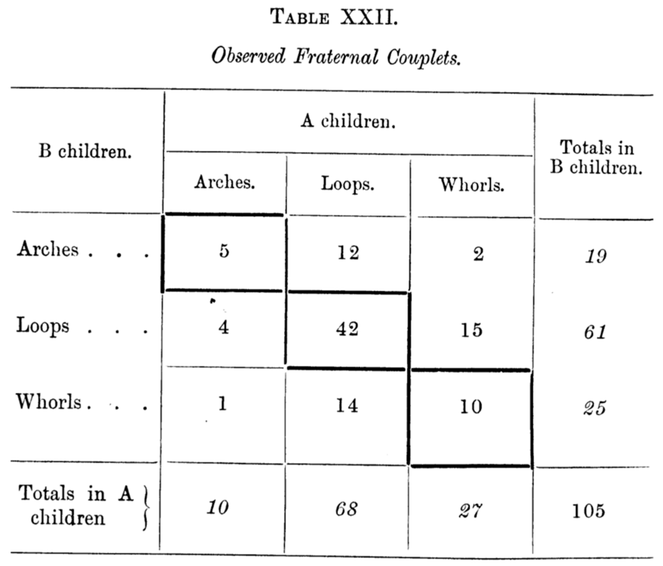
In 1892 Galton [4] published Finger Prints, a book that is considered by some to be the genesis of dactyloscopy; see, for example, Stigler [30], Gillham [31], and Kaldane [32]. By studying a sample of 105 sets of twin brothers, or couplets, Galton [4] was interested in determining the expected number of pairs with distinct fingerprint characteristics (those being arches, whorls, and loops) in their right forefinger; Figure 2 gives a screenshot—from Galton [4] (p. 175)—of the data that Galton analyzed, appearing as a 3 × 3 contingency table. Galton set one set of twin brothers totals to A and the other twin brothers to B and said:

“The question, then, was how far calculations from the above data [Figure 2] would correspond to the contents of [the observed random couplets]. The answer is that it does so admirably. Multiply each of the… A totals into each of the… B totals, and after dividing each result by [n]”

[4] (p. 174)

He then goes on to describe Figure 2 by saying:

“The squares that run diagonally from the top at the left, to the bottom at the right, contain the double events, and it is with these that we are now concerned. Are entries in those squares larger or not than the randoms calculated… viz. the values of 10 $\times$ 19, 68 $\times$ 61, 27 $\times$ 25, all divided by 105?”

[4] (pp. 175–176)

Galton referred to his expected cell frequencies as calculated random couplets, but they now commonly appear, in their simplest form, as:

$$\mathrm{Expected}\mathrm{cell}\mathrm{frequency}={\displaystyle \frac{\mathrm{row}\mathrm{total}\times \mathrm{column}\mathrm{total}}{\mathrm{sample}\mathrm{size}}}.$$

However, Galton’s [4] expected value of the (1, 1)’th cell frequency is just Gilbert’s [17] $e$ which is defined by (4). While Galton was interested in a general expression for this expected value, he was only interested in comparing the observed cell counts with their expected value along the diagonal of his 3 $\times$ 3 table; see the highlighted cell entries along the diagonal of Figure 2. In deriving (3), Gilbert [17] was only concerned with the (1, 1)’th cell of a 2 $\times$ 2 contingency table because he was interested only in verifying the prediction of tornadoes and was not concerned with verifying that tornadoes did not occur. If he had, then Gilbert’s analysis of Finley’s data is comparable in nature to Galton’s interest in his fingerprint data appearing in Figure 2.

It therefore seems reasonable to assign Gilbert [17] some credit for the derivation, justification, and interpretation of the expected cell frequency of a contingency table. Although, some may argue against this since Finley, and Gilbert, did not present or even analyze the data in Figure 1 in the same way that Pearson, Yule, and others analyze a 2 $\times$ 2 contingency table. It is also recognized that Galton’s impact on Pearson’s work is profound and is well documented; see, for example, Gillham [31], Yule and Filon [33], Haldane [34], and Kennedy-Shaffer [35]. One can therefore understand why, during the emergence of statistical thinking that was taking place in the UK at the turn of the 20th century, Gilbert’s [17] definition, justification, and interpretation of his $e$ in 1884—see (4)—would be greatly overshadowed by Galton’s [4] contribution that appeared eight years later. In fact, prior to Pearson’s classic 1904 paper [6], Galton’s expression of the expected cell frequency for Table 1 was also described in 1900 and 1903 by Yule [8] (§16) and Yule [9] (Equation (7)).

4. Peirce’s Analysis

4.1. The “Measure of the Science of the Method” Index

Immediately following Gilbert’s [17] analysis of Finley’s data (in Figure 1), Peirce [18] proposed his own index in 1884. The description of his index starts colorfully by discussing his interest in studying the difference between the observations of an “infallible witness” and those of “an utterly ignorant person”; the latter can be more diplomatically described as observations that would arise purely by chance. Peirce would propose his amendment of Gilbert’s, and Finley’s, index by also denoting it by $i$ and describing it as:

“… the proportion of questions put to the infallible witness”

[18] (p. 453)

It is implied here that the questions put to this “witness” are correctly answered, although his derivation of his index shows a slightly different interpretation. Framing Peirce’s [18] description in terms of Finley’s data, Peirce wanted to determine the difference between correctly and incorrectly predicting that a tornado will occur. Using such terms, his $i$ (we shall denote it as $i_P$) is therefore the proportion of tornadoes correctly predicted, and he referred to it as the measure of the science of the method. He also defined $j$ (here, $j_P$) to be the

“… proportion of questions which the ignorant witness answers in the first way”

[18] (p. 453)

Here, “first way” refers to the witness incorrectly observing the occurrence (or not) of a tornado. Peirce goes on to determine $i_P$ and $j_P$ by solving the following four equations:

$$\begin{gathered} {\mathrm{n}}_{11}=i_P{\mathrm{n}}_{•1}+\left(1-i_P\right)j_P{\mathrm{n}}_{•1}, {\mathrm{n}}_{12}=\left(1-i_P\right)j_P{\mathrm{n}}_{•2} \\ {\mathrm{n}}_{21}=\left(1-i_P\right)\left(1-j_P\right){\mathrm{n}}_{•1}, {\mathrm{n}}_{22}=i_P{\mathrm{n}}_{•2}+\left(1-i_P\right)\left(1-j_P\right){\mathrm{n}}_{•2}. \end{gathered}$$

(5)

The first two equations of (5) can be expressed as the relative cell frequencies of the first row (i.e., the prediction of a tornado) such that:

$${\displaystyle \frac{{\mathrm{n}}_{11}}{{\mathrm{n}}_{•1}}}=i_P+\left(1-i_P\right)j_P, {\displaystyle \frac{{\mathrm{n}}_{12}}{{\mathrm{n}}_{•2}}}=\left(1-i_P\right)j_P$$

and yields the solution to his index:

$$i_P={\displaystyle \frac{{\mathrm{n}}_{11}}{{\mathrm{n}}_{•1}}}-{\displaystyle \frac{{\mathrm{n}}_{12}}{{\mathrm{n}}_{•2}}}.$$

(6)

This is the first way that Peirce [18] defined his index, and it is the difference between the proportion of observed tornadoes that were predicted and the proportion of tornadoes that were not observed but were predicted. Armistead [16] describes (6) as being the difference between the “true positive fraction” (that is, correctly identifying the occurrence of a tornado) and the “false positive fraction” (that is, incorrectly predicting the occurrence of a tornado). Thus, while Section 3.2 has shown that Gilbert’s index for Table 2 is $i_G=0.3846$, Peirce’s [26] measure of the science of the method, (6), is:

$$i_P={\displaystyle \frac{11}{14}}-{\displaystyle \frac{14}{920}}=0.7705.$$

Therefore, Peirce’s index appears to show a stronger positive “link” between the prediction of tornadoes and what was observed when compared with Gilbert’s index. Section 6.7 examines the properties of $i_P$.

4.2. Other Peirce-Type Indices

While Peirce [18] did not give an expression for $j_P$ (that is, an index he denoted by $j$), the second of his four equations in (5) yield:

$$j_P={\displaystyle \frac{{\mathrm{n}}_{12}/{\mathrm{n}}_{•2}}{{\mathrm{n}}_{21}/{\mathrm{n}}_{•1}+{\mathrm{n}}_{12}/{\mathrm{n}}_{•2}}}$$

so that it is the probability of a predicted tornado not occurring given that the predictions made are incorrect.

The last two equations of (5) can also be expressed as relative cell frequencies of the second row (i.e., the prediction of a tornado not occurring) so that:

$${\displaystyle \frac{{\mathrm{n}}_{21}}{{\mathrm{n}}_{•1}}}=\left(1-i_P\right)\left(1-j_P\right) {\displaystyle \frac{{\mathrm{n}}_{22}}{{\mathrm{n}}_{•2}}}=i_P+\left(1-i_P\right)\left(1-j_P\right).$$

So, while Peirce did not show this, $i_P$ can also be defined as:

$$i_P={\displaystyle \frac{{\mathrm{n}}_{22}}{{\mathrm{n}}_{•2}}}-{\displaystyle \frac{{\mathrm{n}}_{21}}{{\mathrm{n}}_{•1}}}$$

(7)

which is the difference between the proportion of tornadoes that did not occur but were (correctly) not predicted and the proportion of tornadoes that were observed but were not predicted. For Table 2, (7) confirms that:

$$i_P={\displaystyle \frac{906}{920}}-{\displaystyle \frac{3}{14}}=0.7705.$$

Simultaneously solving all four of Peirce’s equations in (5) yields the solution:

$$i_P={\displaystyle \frac{{\mathrm{n}}_{11}{\mathrm{n}}_{22}-{\mathrm{n}}_{12}{\mathrm{n}}_{21}}{{\mathrm{n}}_{•1}{\mathrm{n}}_{•2}}}$$

which is identical to Youden’s [36] (p. 33) J-index of 1950. Youden’s motivation for deriving his index was the same as Peirce’s but their contexts were very different. While Peirce was concerned with correctly identifying that a predicted tornado occurred, Youden was concerned with correctly identifying that someone was diagnosed with having a disease. This last definition of the index also gives $i_P=0.7705$ for Table 2.

Rovine and Anderson [14] note that $i_P$ has the hallmarks of a coefficient of association described by Yule [8]. These being that $i_P=0$ when the two variables are independent—since ${\mathrm{n}}_{11}{\mathrm{n}}_{22}={\mathrm{n}}_{12}{\mathrm{n}}_{21}$; a property akin to an odds ratio of 1, and a feature of independence described by Yule [8] (§19). Additionally, $i_P=1$ when there is perfect positive association and $i_P=-1$ when there is perfect negative association; more will be said on these features in Section 6.7. In fact, in the case where ${\mathrm{n}}_{1•}={\mathrm{n}}_{•1}$ and ${\mathrm{n}}_{2•}={\mathrm{n}}_{•2},$ then (6), and hence (7), is equivalent to the square root of Pearson’s [6] (Equation (xxviii)) mean square contingency, a quantity I briefly speak of in Section 5.2.

5. Doolittle’s Analysis

5.1. The “Degree of Logical Connection” Index

Following on from Finley’s [12] study of his tornado data and Gilbert’s [17] response to this work, further improvements were undertaken by Doolittle [19] in 1885. Doolittle adopted the same notation used by Gilbert and introduced his paper by saying:

“Mr G. K. Gilbert has published… a method of estimating the ratio of skill in predictions of occurrences and non-occurrences of a simple event.”

[19] (p. 122)

While Doolittle refers to “a simple event” he derives his index in general terms before analyzing Finley’s tornado data. Doolittle [19] (p. 123) then describes that the probability of “success is proportional” to ${\mathrm{n}}_{11}/{\mathrm{n}}_{1•}$ and ${\mathrm{n}}_{11}/{\mathrm{n}}_{•1}$; here he is talking about the proportion of successfully predicted tornadoes to occur AND, based on the predictions that are made, the proportion of tornadoes that occurred, respectively. Therefore, Doolittle [19] defined the index by:

$$s_D={\displaystyle \frac{{\mathrm{n}}_{11}}{{\mathrm{n}}_{•1}}}·{\displaystyle \frac{{\mathrm{n}}_{11}}{{\mathrm{n}}_{1•}}}$$

(8)

which he refers to as the proportion of “successful” predictions. For Table 2,

$$s_D={\displaystyle \frac{11}{14}}·{\displaystyle \frac{11}{25}}=0.3457.$$

Doolittle was aware that (8) does not accommodate for the possibility of observations happening by “chance” but does say that:

“The fraction $\left[{\mathrm{n}}_{•1}/\mathrm{n}\right]$ represents the ratio of random success and therefore $\left[{\mathrm{n}}_{•1}{\mathrm{n}}_{1•}/\mathrm{n}\right]$ verifications out of $\left[{\mathrm{n}}_{1•}\right]$ predictions are to be ascribed to chance and must be subtracted throughout.”

[19] (p. 123)

There are two things to note here. Firstly, he is saying that of the ${\mathrm{n}}_{•1}$ predicted tornadoes, there are ${\mathrm{n}}_{•1}{\mathrm{n}}_{1•}/\mathrm{n}$ of them that occur by “chance”. This is precisely Gilbert’s $e$ and, hence, Galton’s [4] way of calculating the expected number of correctly predicted tornadoes to be observed—if the predicted number of tornadoes and the observed number of tornadoes—was completely independent. Secondly, by saying “throughout”, Doolittle is referring to the numerator and denominator of (8). Thus, Doolittle subtracts ${\mathrm{n}}_{•1}{\mathrm{n}}_{1•}/\mathrm{n}$ “throughout” and in doing so follows the same tact that Gilbert used when he derived his index, $i_G$; see (3). That is, Doolittle amended (8) so that it is of the form:

$$i_{\mathrm{D}}={\displaystyle \frac{{\mathrm{n}}_{11}-\frac{{\mathrm{n}}_{1•}{\mathrm{n}}_{•1}}{\mathrm{n}}}{{\mathrm{n}}_{•1}-\frac{{\mathrm{n}}_{1•}{\mathrm{n}}_{•1}}{\mathrm{n}}}}·{\displaystyle \frac{{\mathrm{n}}_{11}-\frac{{\mathrm{n}}_{1•}{\mathrm{n}}_{•1}}{\mathrm{n}}}{{\mathrm{n}}_{1•}-\frac{{\mathrm{n}}_{1•}{\mathrm{n}}_{•1}}{\mathrm{n}}}}$$

(9)

which he referred to as the degree of logical connection between the observed number of tornadoes and the predicted number of tornadoes. It is at this point that he also gives an alternative form of this revised index showing that (9) is also equivalent to:

$$i_{\mathrm{D}}={\displaystyle \frac{{\left(\mathrm{n}{\mathrm{n}}_{11}-{\mathrm{n}}_{1•}{\mathrm{n}}_{•1}\right)}^2}{{\mathrm{n}}_{1•}{\mathrm{n}}_{•1}\left(\mathrm{n}-{\mathrm{n}}_{1•}\right)\left(\mathrm{n}-{\mathrm{n}}_{•1}\right)}}$$

(10)

which can also be written as:

$$i_{\mathrm{D}}={\mathrm{n}}^2{\displaystyle \frac{{\left({\mathrm{n}}_{11}-\frac{{\mathrm{n}}_{1•}{\mathrm{n}}_{•1}}{\mathrm{n}}\right)}^2}{{\mathrm{n}}_{1•}{\mathrm{n}}_{•1}{\mathrm{n}}_{2•}{\mathrm{n}}_{•2}}}.$$

Therefore, Doolittle’s revision of Gilbert’s index for Table 2 gives an index value that is comparable to his own $s_D=0.3457$ and Gilbert’s index (of $i_G=0.3929$) where, using (10),

$$i_{\mathrm{D}}={\displaystyle \frac{{\left(934·11-25·14\right)}^2}{25·14·\left(934-25\right)\left(934-14\right)}}=0.3365$$

but differs substantially to Peirce’s index of $i_P=0.7705$. Like $i_{\mathrm{G}}$ and $i_{\mathrm{P}}$, when the variables of Table 1 are independent (9) and (10) shows that $i_{\mathrm{D}}=0$.

Doolittle then proceeds to derive (10) a second way. This time noting that (and keeping to his spelling and the notation outlined in Table 1):

“Since the skillful predictions are mingled indistinguishably with all the unskilled ones, and are vitiated accordingly, the value of the vitiated probability of the skillful prediction of any single occurrence may be represented by the product

$$i_{\mathrm{D}}=\left({\displaystyle \frac{{\mathrm{n}}_{11}}{{\mathrm{n}}_{•1}}}-{\displaystyle \frac{{\mathrm{n}}_{1•}-{\mathrm{n}}_{11}}{\mathrm{n}-{\mathrm{n}}_{•1}}}\right)\left({\displaystyle \frac{{\mathrm{n}}_{11}}{{\mathrm{n}}_{1•}}}-{\displaystyle \frac{{\mathrm{n}}_{•1}-{\mathrm{n}}_{11}}{\mathrm{n}-{\mathrm{n}}_{1•}}}\right)={\displaystyle \frac{{\left(\mathrm{n}{\mathrm{n}}_{11}-{\mathrm{n}}_{1•}{\mathrm{n}}_{•1}\right)}^2}{{\mathrm{n}}_{1•}{\mathrm{n}}_{•1}\left(\mathrm{n}-{\mathrm{n}}_{1•}\right)\left(\mathrm{n}-{\mathrm{n}}_{•1}\right)}}.”$$

[19] (p. 124)

By saying vitiated, Doolittle concedes that determining the probability of making a successful prediction is “spoiled” by any randomness that may exist in the process of calculating a successful outcome. Therefore, he deals with this “spoiled” prediction by removing it from the observed number of successful predictions, just as Gilbert did. This can be seen by rewriting $i_{\mathrm{D}}$ in a slightly different, but equivalent, way:

$$i_{\mathrm{D}}=\left({\displaystyle \frac{{\mathrm{n}}_{11}}{{\mathrm{n}}_{•1}}}-{\displaystyle \frac{{\mathrm{n}}_{12}}{{\mathrm{n}}_{•2}}}\right)\left({\displaystyle \frac{{\mathrm{n}}_{11}}{{\mathrm{n}}_{1•}}}-{\displaystyle \frac{{\mathrm{n}}_{21}}{{\mathrm{n}}_{2•}}}\right).$$

We can see here that this index removes from the two probabilities of “success” of predictions and observations their associated probabilities of “failure” and yields a value of $i_{\mathrm{D}}=0.3365$, just like his other expressions of $i_{\mathrm{D}}$.

5.2. Doolittle and the Mean Square Contingency

One may note that Peirce’s $s_{\mathrm{D}}$, (8), (of 1885) is equivalent to the (1, 1)’th element of the partition of Pearson’s [6] (Equation (xxviii)) mean square contingency (of 1904):

$${\varphi }^2={\displaystyle \frac{{\mathrm{X}}^2}{\mathrm{n}}}=\sum _{\mathrm{j}=1}^2\sum _{\mathrm{i}=1}^2\left({\displaystyle \frac{{\mathrm{n}}_{\mathrm{i}\mathrm{j}}}{{\mathrm{n}}_{\mathrm{i}•}}}·{\displaystyle \frac{{\mathrm{n}}_{\mathrm{i}\mathrm{j}}}{{\mathrm{n}}_{•\mathrm{j}}}}\right)-1$$

where ${\mathrm{X}}^2$ is Pearson’s chi-squared statistic of Table 1, not including Yates’ [37] continuity correction. Therefore, there is a thread of agreement as well as substantial differences with the way Doolittle viewed his measure of “success” and how Pearson derives his mean square contingency for a contingency table. Doolittle was only interested in the (1, 1)’th element of Table 1 while Pearson was concerned with all elements of a larger sized table. This difference comes about by how Doolittle and Pearson viewed their analysis of categorical data. Like Gilbert, Doolittle was only concerned with the verification of the tornadoes that were predicted to occur and so confined his attention to the (1, 1)’th cell frequency. On the other hand, Pearson was more interested in general measures of association and so was concerned with ALL cell frequencies. If Doolittle had considered determining his index for all four elements, then perhaps he would have simply summed his terms (being the simplest of operations) resulting in an emended version of (8):

$${\tilde{s}}_D={\displaystyle \frac{{\mathrm{n}}_{11}}{{\mathrm{n}}_{1•}}}·{\displaystyle \frac{{\mathrm{n}}_{11}}{{\mathrm{n}}_{•1}}}+{\displaystyle \frac{{\mathrm{n}}_{12}}{{\mathrm{n}}_{1•}}}·{\displaystyle \frac{{\mathrm{n}}_{12}}{{\mathrm{n}}_{•2}}}+{\displaystyle \frac{{\mathrm{n}}_{21}}{{\mathrm{n}}_{2•}}}·{\displaystyle \frac{{\mathrm{n}}_{21}}{{\mathrm{n}}_{•1}}}+{\displaystyle \frac{{\mathrm{n}}_{22}}{{\mathrm{n}}_{2•}}}·{\displaystyle \frac{{\mathrm{n}}_{22}}{{\mathrm{n}}_{•2}}}$$

where the first term on the right-hand side is just (8). Note that ${\tilde{s}}_D$ is equivalent to ${\varphi }^2+1$ for Table 1. Therefore, predicting a tornado purely by “chance” would mean that, ${\tilde{s}}_D=1$ so that any deviation away from 1 would show that there was some merit in the prediction process.

It can be established that Doolittle’s index $i_{\mathrm{D}}$ is far more closely aligned to Pearson’s mean square contingency than ${\tilde{s}}_D$. Examining (10) more carefully, it can also be written as:

$$i_{\mathrm{D}}={\displaystyle \frac{{\left({\mathrm{n}}_{11}{\mathrm{n}}_{22}-{\mathrm{n}}_{12}{\mathrm{n}}_{21}\right)}^2}{{\mathrm{n}}_{1•}{\mathrm{n}}_{•1}{\mathrm{n}}_{2•}{\mathrm{n}}_{•2}}}$$

which is Pearson’s [6] (Equation (xxviii)) mean square contingency! That is $i_{\mathrm{D}}={\varphi }^2$. Thus, it certainly appears that Doolittle proposed the famous mean square contingency (albeit, in context of a 2 $\times$ 2 contingency table) nearly 20 years prior to Pearson’s publication of the statistic, although the nature of its derivation differs. Perhaps if Doolittle was concerned with not just the vitiated proportion of successes but also considered the vitiated number of successful predictions he would have been apportioned some credit to the early development of the chi-squared statistic, at least for the 2 $\times$ 2 contingency table.

One may also note that $i_{\mathrm{D}}$ is the square of $\varphi$, where

$$\varphi ={\displaystyle \frac{{\mathrm{n}}_{11}{\mathrm{n}}_{22}-{\mathrm{n}}_{12}{\mathrm{n}}_{21}}{\sqrt{{\mathrm{n}}_{1•}{\mathrm{n}}_{•1}{\mathrm{n}}_{2•}{\mathrm{n}}_{•2}}}}$$

is Pearson’s phi correlation—see [38] (Equation (xxxviii)) and [39] (p. 167)—or phi coefficient [40] (Equation (6.2)) whose value ranges between −1 and +1 (inclusive). This quantity is also equivalent to Matthews’ correlation coefficient [41] and is used in a variety of disciplines including, but certainly not confined to, bioscience, medical science and machine learning literatures.

What should also be apparent is that the link between Peirce’s index (6) and Doolittle’s index (10) is:

$$i_{\mathrm{D}}=i_P^2\left({\displaystyle \frac{{\mathrm{n}}_{•1}{\mathrm{n}}_{•2}}{{\mathrm{n}}_{1•}{\mathrm{n}}_{2•}}}\right)$$

so that the square of Peirce’s index is proportional to Pearson’s chi-squared statistic of Table 1 since:

$${\mathrm{X}}^2=\mathrm{n}{i}_{\mathrm{D}}=\mathrm{n}{i}_P^2\left({\displaystyle \frac{{\mathrm{n}}_{•1}{\mathrm{n}}_{•2}}{{\mathrm{n}}_{1•}{\mathrm{n}}_{2•}}}\right).$$

When analyzing Finley’s data that is summarized in Figure 1 (except for May (8-h)), ${\mathrm{n}}_{•1}\approx 2{\mathrm{n}}_{•1}$ and ${\mathrm{n}}_{2•}\approx {\mathrm{n}}_{•2}$ so that ${\mathrm{X}}^2=\mathrm{n}{i}_{\mathrm{D}}\approx 0.5\mathrm{n}{i}_P^2$. This can be verified by noting that, for Table 2, ${\mathrm{X}}^2=314.3$ (without Yates’ continuity correction), $\mathrm{n}{i}_{\mathrm{D}}=934·0.3365=314.3$ and $0.5\mathrm{n}{i}_P^2=0.5·934·{0.7705}^2=277.2;$ since $\left({\mathrm{n}}_{•1}{\mathrm{n}}_{•2}\right)/\left({\mathrm{n}}_{1•}{\mathrm{n}}_{2•}\right)=\left(14·920\right)/\left(25·909\right)=0.5668$, and not 0.5, then $\mathrm{n}\left(\left({\mathrm{n}}_{•1}{\mathrm{n}}_{•2}\right)/\left({\mathrm{n}}_{1•}{\mathrm{n}}_{2•}\right)\right)i_P^2=314.3$, as expected.

6. Further Evaluations of the Indices

6.1. Some Preliminary Features of Table 2

With the various indices now derived and described, our attention turns to delving deeper into some of their features. To do this we evaluate the indices across the full range of values that ${\mathrm{n}}_{11}$ can take. This will be done by assuming that the marginal frequencies of Table 1 are known and fixed so that ${\mathrm{n}}_{11}$ lies within the Fréchet [42]-type bounds:

$$\mathrm{L}=\mathrm{m}\mathrm{a}\mathrm{x}\left(0, {\mathrm{n}}_{•1}-{\mathrm{n}}_{2•}\right)\le {\mathrm{n}}_{11}\le \mathrm{m}\mathrm{i}\mathrm{n}\left({\mathrm{n}}_{1•}, {\mathrm{n}}_{•1}\right)=\mathrm{U}.$$

(11)

For Table 2, ${\mathrm{n}}_{11}\in \left[0,14\right]$. Since the expected value of the (1, 1)’th cell under independence (that is, Gilbert’s $e$) plays an important role in the definition of some of the indices, for Table 2 it is:

$$e={\displaystyle \frac{25·14}{934}}=0.3747$$

and is very small in comparison to the observed (1, 1)’th cell frequency of 11. On the surface, this suggests that there are more tornadoes correctly predicted than what would be expected if the predictions were, using the terms of Gilbert, Peirce, and Doolittle, made “fortuitously”, by “chance”, or by “coincidence”. However, the large sample size (relative to ${\mathrm{n}}_{11}=14$) is accounted for by the very large (2, 2)’th cell frequency and helps to undervalue $e$ thereby exacerbating the points raised by “G” [27] (p. 126) and Gilbert [17] (p. 166). For the March, May (8-h observation), and May (10-h observation) data sets, $e$ is extremely small compared to its ${\mathrm{n}}_{11}$ and sample size, being 0.7250, 0.2509 and 0.4007, respectively. Aggregating the four data sets produces $e=1.8195$.

Confirmation of the statistical significance of the association between the Prediction and Occurrence variables of Table 2 can be made by performing a chi-squared test of independence. This will be done without using Yates’ continuity correction [37] since his correction came several decades after the work of Galton, Pearson, and the US quartet that is central to this discussion. Pearson’s chi-squared statistic can be expressed in terms of only ${\mathrm{n}}_{11}$ and the marginal frequencies by:

$${\mathrm{X}}^2\left({\mathrm{n}}_{11}\right)=\mathrm{n}{\left({\displaystyle \frac{{\mathrm{n}}_{11}-{\mathrm{n}}_{1•}{\mathrm{n}}_{•1}}{{\mathrm{n}}_{1•}{\mathrm{n}}_{2•}}}\right)}^2\left({\displaystyle \frac{{\mathrm{n}}_{1•}{\mathrm{n}}_{2•}}{{\mathrm{n}}_{•1}{\mathrm{n}}_{•2}}}\right)$$

and is a quadratic function of ${\mathrm{n}}_{11}$ Thus, with ${\mathrm{n}}_{11}=11$, Pearson’s chi-squared statistic for Table 2 is:

$${\mathrm{X}}^2\left(11\right)=934{\left({\displaystyle \frac{11-25·14}{25·909}}\right)}^2\left({\displaystyle \frac{25·909}{14·920}}\right)=314.268$$

so that it has a p-value that is less than 0.001. Therefore, there is enough evidence in the sample to conclude that there is a statistically significant association between the prediction of tornadoes and the observed tornadoes. However, since ${\mathrm{X}}^2\left({\mathrm{n}}_{11}\right)$ is linearly related to $\mathrm{n}$, the large sample size (again, relative to ${\mathrm{n}}_{11}$) helps to inflate the value of the chi-squared statistic. To accommodate this feature, many in the statistics literature, including Mosteller [43] and Mirkin [44], propose dividing the statistic by its sample size. Dividing ${\mathrm{X}}^2\left({\mathrm{n}}_{11}\right)$ by $\mathrm{n}$ gives Pearson’s [6] mean square contingency, ${\varphi }^2$, and, equivalently (since our focus here is on the analysis of Table 1), Doolittle’s $i_{\mathrm{D}}$.

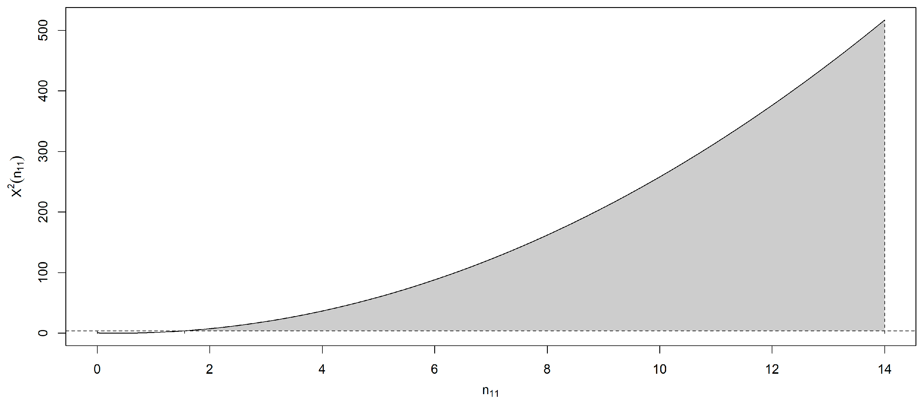
Figure 3 shows the relationship between ${\mathrm{n}}_{11}\in \left[0,14\right]$ and ${\mathrm{X}}^2\left({\mathrm{n}}_{11}\right)$ for Table 2 where the shaded region identifies where a statistically significant association exists between the variables of Table 2. This shaded region is based, in part, on the interval:

$${\mathrm{L}}_{\mathsf{\alpha }}=\mathrm{m}\mathrm{a}\mathrm{x}\left(0, {\displaystyle \frac{{{\mathrm{n}}_{1•}\mathrm{n}}_{•1}}{\mathrm{n}}}-{\displaystyle \frac{{{\mathrm{n}}_{1•}\mathrm{n}}_{2•}}{\mathrm{n}}}\sqrt{{\displaystyle \frac{{\mathsf{\chi }}_{\mathsf{\alpha }}^2}{\mathrm{n}}}{\displaystyle \frac{{\mathrm{n}}_{1•}{\mathrm{n}}_{2•}}{{\mathrm{n}}_{•1}{\mathrm{n}}_{•2}}}}\right)<{\mathrm{n}}_{11}<\mathrm{m}\mathrm{i}\mathrm{n}\left({\mathrm{n}}_{1•}, {\displaystyle \frac{{{\mathrm{n}}_{1•}\mathrm{n}}_{•1}}{\mathrm{n}}}+{\displaystyle \frac{{\mathrm{n}}_{1•}{\mathrm{n}}_{2•}}{\mathrm{n}}}\sqrt{{\displaystyle \frac{{\mathsf{\chi }}_{\mathsf{\alpha }}^2}{\mathrm{n}}}{\displaystyle \frac{{\mathrm{n}}_{1•}{\mathrm{n}}_{2•}}{{\mathrm{n}}_{•1}{\mathrm{n}}_{•2}}}}\right)={\mathrm{U}}_{\mathsf{\alpha }}$$

where ${\mathsf{\chi }}_{\mathsf{\alpha }}^2$ is the $1-\mathsf{\alpha }$ percentile of the chi-squared distribution with one degree of freedom. This is the interval of ${\mathrm{n}}_{11}$ where no statistically significant association exists and is an adaptation of the interval derived by Beh [45] for the conditional proportion ${\mathrm{P}}_1={\mathrm{n}}_{11}/{\mathrm{n}}_{1•}$. When testing the association between the Predictions and Occurrence variables of Table 2 at the $\mathsf{\alpha }=0.05$ level of significance, a statistically significant association exists for ${\mathrm{n}}_{11}$ lying outside interval [1.549, 14] which is a very small region since ${\mathrm{n}}_{11}\in \left[0,14\right]$. The dominance of the (2, 2)’th cell frequency plays a pivotal role in the calculation of this interval.

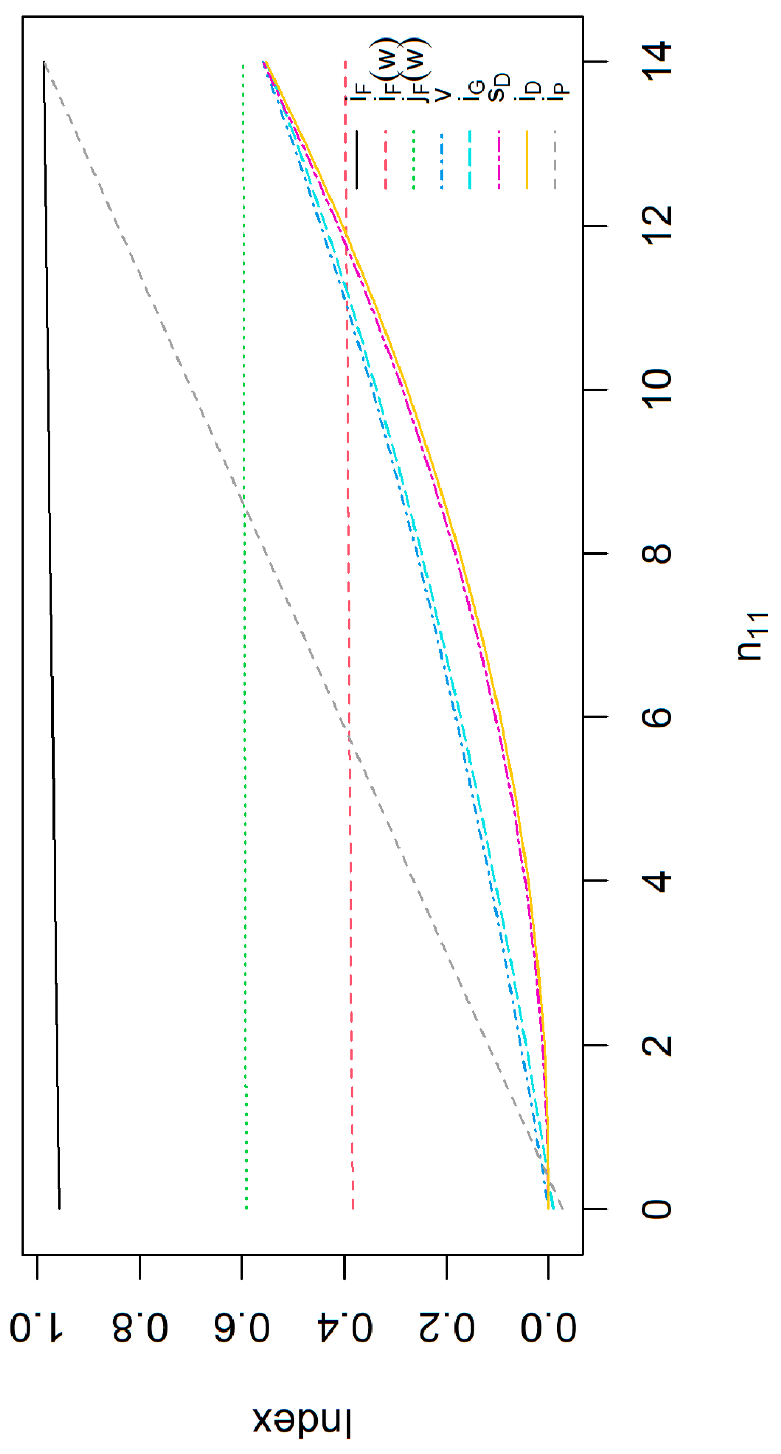
A comparison of the six indices—$i_F$, $v$, $i_G$, $i_P$, $s_{D,}$ and $i_D$—plus two weighted versions of $i_F$ is given in Figure 4 for Table 2 where ${\mathrm{n}}_{11}\in \left[0,14\right]$. I shall now discuss some of the key features of these indices and discuss their behavior in terms of ${\mathrm{n}}_{11}$. Summarized in

Table 3. Value of each observed index, their value under independence, and the interval of possible values it takes for the four data sets and their aggregation in Figure 1.

Index/Month	Index	Independence	Bounds
$i_F$
March	0.9429	0.9292	[0.9274, 0.9611]
April	0.9818	0.9590	[0.9582, 0.9882]
May (8 h)	0.9857	0.9579	[0.9570, 0.9928]
May (10 h)	0.9519	0.9422	[0.9407, 0.9778]
Aggregate	0.9661	0.9474	[0.9461, 0.9825]
$i_F\left(0.6\right)$
March	0.3787	0.3719	[0.3709, 0.3878]
April	0.3951	0.3837	[0.3833, 0.3983]
May (8 h)	0.3971	0.3832	[0.3828, 0.4007]
May (10 h)	0.3819	0.3771	[0.3763, 0.3948]
Aggregate	0.3884	0.3791	[0.3785, 0.3966]
$j_F\left(0.6\right)$
March	0.5886	0.5858	[0.5855, 0.5922]
April	0.5964	0.5918	[0.5916, 0.5976]
May (8 h)	0.5971	0.5916	[0.5914, 0.5986]
May (10 h)	0.5904	0.5884	[0.5881, 0.5956]
Aggregate	0.5932	0.5895	[0.5892, 0.5965]
$v$
March	0.1200	0.0131	[0, 0.3023]
April	0.3929	0.0097	[0, 0.5600]
May (8 h)	0.5000	0.0106	[0, 0.7143]
May (10 h)	0.1034	0.0129	[0, 0.4545]
Aggregate	0.2276	0.0122	[0, 0.5100]
$i_G$
March	0.1071	0	[−0.0131, 0.2904]
April	0.3846	0	[−0.0097, 0.5533]
May (8 h)	0.4920	0	[−0.0106, 0.7091]
May (10 h)	0.0907	0	[−0.0129, 0.4443]
Aggregate	0.2160	0	[−0.0122, 0.5009]
$i_P$
March	0.4127	0	[−0.0567, 0.9604]
April	0.7705	0	[−0.0272, 0.9880]
May (8 h)	0.5678	0	[−0.0184, 0.7143]
May (10 h)	0.2642	0	[−0.0415, 0.9774]
Aggregate	0.5229	0	[−0.0363, 0.9822]
$s_{\mathrm{D}}$
March	0.0644	0.0009	[0, 0.3023]
April	0.3457	0.0004	[0, 0.5600]
May (8 h)	0.4571	0.0004	[0, 0.7143]
May (10 h)	0.0409	0.0008	[0, 0.4545]
Aggregate	0.1537	0.0006	[0, 0.5100]
$i_{\mathrm{D}}$
March	0.0536	0	[0.0001, 0.2904]
April	0.3365	0	[0.0004, 0.5533]
May (8 h)	0.4480	0	[0.0005, 0.7091]
May (10 h)	0.0325	0	[0.0008, 0.4443]
Aggregate	0.1420	0	[0, 0.5009]

is the value of each index, its bounds, and the value of the index under the assumption of independence between Predictions and Occurrence for the four data sets in Figure 1.

6.2. Features of Finley’s $i_F$

Suppose we consider Finley’s index $i_F$; see (1). Some algebra shows that it can be alternatively, and equivalently, expressed as:

$$i_F={\displaystyle \frac{2}{\mathrm{n}}}{\mathrm{n}}_{11}+{\displaystyle \frac{{\mathrm{n}}_{2•}-{\mathrm{n}}_{•1}}{\mathrm{n}}}$$

so that $i_F$ is a linear function of ${\mathrm{n}}_{11}$. This alternative expression tells us that, when analyzing Finley’s data, since ${\mathrm{n}}_{2•}$ is very large in comparison to ${\mathrm{n}}_{•1}$ and any value that ${\mathrm{n}}_{11}$ can take, then $i_F\approx {\mathrm{n}}_{2•}/\mathrm{n}\lesssim 1$. Here “$\lesssim$ ” is used here to mean “less than but approximately equal to”; for example, $1.9876\lesssim 2$. For Table 2:

$$i_F=0.002{\mathrm{n}}_{11}+0.9582$$

so that $i_F\in \left[0.9582,0.9862\right]\lesssim 1$ for all ${\mathrm{n}}_{11}\in \left[0, 14\right]$; this interval is reflected by the solid black line in Figure 4. Since the bounds of ${\mathrm{n}}_{11}$ are given by (11), the bounds of (1) are:

$${\mathrm{L}}_F={\displaystyle \frac{{\mathrm{n}}_{2•}-{\mathrm{n}}_{1•}}{\mathrm{n}}}\le i_F\le 1+\mathrm{m}\mathrm{i}\mathrm{n}\left(0,{\displaystyle \frac{2\left({\mathrm{n}}_{•1}-{\mathrm{n}}_{1•}\right)}{\mathrm{n}}}\right)={\mathrm{U}}_F.$$

For Finley’s data ${\mathrm{n}}_{2•}\gg {\mathrm{n}}_{1•}$, ${\mathrm{n}}_{2•}\lesssim \mathrm{n}$ and ${\mathrm{n}}_{1•}\approx {\mathrm{n}}_{•1}$ so that ${\mathrm{L}}_F\lesssim i_F\lesssim {\mathrm{U}}_F\lesssim 1$ where ${\mathrm{L}}_F$ is less than (but still very close to) 1. So, the observed value of $i_{\mathrm{F}}=0.9818$ lies close to its upper bound suggesting that the predictions made by Finley are vastly better than if the predictions were made by chance. However, such a conclusion would also be valid for ANY value that ${\mathrm{n}}_{11}$ can take in the interval $\left[0, 14\right]$. Therefore, since the lower and upper bounds of $i_{\mathrm{F}}$ are both very close to 1, irrespective of how many tornadoes were predicted and observed, an analysis of Finley’s April 1884 data using his index will mean that his predictions will ALWAYS be viewed as extremely accurate. In fact, even if none of his predictions occurred, so that ${\mathrm{n}}_{11}=0$, then $i_F=0.9582$! Clearly the very large values that Finley’s index take across ${\mathrm{n}}_{11}\in \left[0, 14\right]$ shows how poor a quantity $i_F$ is. This behavior in the index is also observed for the March, May (8-h observation), and May (10-h observation) predictions and observations Finley made; the bounds of his index for these data sets are very similar to the bounds of his April records and are $\left[0.9274, 0.9611\right]$, $\left[0.9570, 0.9928\right]$ and $\left[0.9407, 0.9778\right]$, respectively. Aggregating the cell frequencies of the four tables in Figure 1 yields the bounds for Finley’s index $i_F\in \left[0.9461, 0.9825\right]$.

When the row and column variables of Table 1 are independent, Finley’s index, (1), is:

$$\begin{array}{cc}\hfill i_{F|I}& ={\displaystyle \frac{2}{\mathrm{n}}}e+{\displaystyle \frac{{\mathrm{n}}_{2•}-{\mathrm{n}}_{•1}}{\mathrm{n}}}\hfill \\ & ={\displaystyle \frac{2}{\mathrm{n}}}·{\displaystyle \frac{{\mathrm{n}}_{1•}{\mathrm{n}}_{•1}}{\mathrm{n}}}+{\displaystyle \frac{{\mathrm{n}}_{2•}-{\mathrm{n}}_{•1}}{\mathrm{n}}}\hfill \end{array}$$

where the addition of “|I” to the subscript indicates the index is calculated assuming there is independence between the Prediction and Occurrence variables of Table 1. Therefore, for Table 2:

$$i_{F|I}={\displaystyle \frac{2}{934}}·{\displaystyle \frac{25·14}{934}}+{\displaystyle \frac{909-14}{934}}=0.9590$$

which lies near the lower bound of the interval $\left[0.9582, 0.9882\right]$. This should be of no surprise since $e=0.3747$ lies close to the lower bound of the range of values ${\mathrm{n}}_{11}$ can take for Table 2.

6.3. A Weighted Finley Index (Version 1)

Gilbert remarked in his 1884 paper [17] on the flaw induced by the large value of ${\mathrm{n}}_{22}$ when calculating Finley’s index, (1), by saying:

“This fallacy consists in the assumption that verification of the predictions of a rare event may be classed with verifications of the predictions of frequent events, without any system of weighting.”

[17] (p. 166)

Gilbert did not propose a weighted version of (1) but two simple adaptations of Finley’s index will be discussed. I concede that there may well be various other ways in which a weighted Finley index can be defined but the first one I examine is:

$$i_F\left(w\right)={\displaystyle \frac{w{\mathrm{n}}_{11}+\left(1-w\right){\mathrm{n}}_{22}}{\mathrm{n}}}$$

(12)

for a given weight $w\in \left[0, 1\right]$. This index allows one to weigh the predictions of a rare event (tornadoes occurring) and a frequent event (tornado not occurring) differently. It is immediately clear that if ${\mathrm{n}}_{11}$ and ${\mathrm{n}}_{22}$ were given equal weighting so that $w=0.5$ then $i_F\left(0.5\right)=0.5i_F$. However, regardless of the choice of $w$, $i_F>i_F\left(w\right)$ and this seems, on the surface, to be an acceptable feature since $i_F>0.95$ for ${\mathrm{n}}_{11}\in \left[0, 14\right]$. Equation (12) can be alternatively expressed as a linear function of $w$ by:

$$\begin{array}{cc}\hfill i_F\left(w\right)& =w\left({\displaystyle \frac{{\mathrm{n}}_{11}-{\mathrm{n}}_{22}}{\mathrm{n}}}\right)+{\displaystyle \frac{{\mathrm{n}}_{22}}{\mathrm{n}}}\hfill \\ & =-w\left({\displaystyle \frac{{\mathrm{n}}_{2•}-{\mathrm{n}}_{•1}}{\mathrm{n}}}\right)+\left({\displaystyle \frac{{\mathrm{n}}_{11}+{\mathrm{n}}_{2•}-{\mathrm{n}}_{•1}}{\mathrm{n}}}\right).\hfill \end{array}$$

Since ${\mathrm{n}}_{11}\ll {\mathrm{n}}_{22}$ or, alternatively, because ${\mathrm{n}}_{•1}\ll {\mathrm{n}}_{2•}$, this relationship shows that the coefficient of $w$ is, approximately, $-1$ with an intercept of, approximately, $+1$ so that:

$$i_F\left(w\right)\approx -w+1.$$

For example, the relationship between $i_F\left(w\right)$ and $w$ for Table 2 is:

$$i_F\left(w\right)\approx -0.9582w+0.9700.$$

Unsurprisingly, $i_F\left(0.5\right)=0.4909$ for Table 2; exactly half of the $i_F=0.9818$ value. Additionally, since $w\in \left[0, 1\right],$ then $i_F\left(w\right)\in \left[0.0118, 0.9700\right]$, but this interval is dominated more by the chosen value of $w$ than on the cell frequencies of Table 2.

The weighted Finley index, (12), can also be written as a linear function of ${\mathrm{n}}_{11}$ by:

$$i_F\left({\mathrm{n}}_{11}|w\right)={\displaystyle \frac{1}{\mathrm{n}}}{\mathrm{n}}_{11}+\left(1-w\right)\left({\displaystyle \frac{{\mathrm{n}}_{2•}-{\mathrm{n}}_{•1}}{\mathrm{n}}}\right).$$

This function shows that the influence of ${\mathrm{n}}_{11}$ to changes in the index is very small—only $1/\mathrm{n}$ since the sample size for each of Finley’s data sets is quite large. This corroborates the feature that the impact of the cell frequencies on $i_F\left(w\right)$ is negligible so that the weighted index is dominated by $w$. For Table 2, this relationship is:

$$i_F\left({\mathrm{n}}_{11}|w\right)=0.0011{\mathrm{n}}_{11}+0.9582\left(1-w\right)\approx -w+1.$$

For example,

$$i_F\left({\mathrm{n}}_{11}|0.6\right)=0.0011{\mathrm{n}}_{11}+0.3833\lesssim 0.4$$

which is depicted by the red dashed line in Figure 4. Therefore, by weighing the (1, 1)’th and (2, 2)’th cell frequencies of Finley’s data like (12), this shows that $i_F\left(w\right)$ really is of no additional benefit when it is compared to (1). To further assess whether $i_F\left(w\right)$ is of greater utility (or not) than Finley’s index, (12) is bounded by:

$$0\le {\mathrm{L}}_{F|w}={\displaystyle \frac{\left(1-w\right)\left({\mathrm{n}}_{2•}-{\mathrm{n}}_{•1}\right)}{\mathrm{n}}}\le i_F\left(w\right)\le {\displaystyle \frac{\mathrm{m}\mathrm{i}\mathrm{n}\left({\mathrm{n}}_{1•}, {\mathrm{n}}_{•1}\right)}{\mathrm{n}}}+{\displaystyle \frac{\left(1-\mathrm{w}\right)\left({\mathrm{n}}_{2•}-{\mathrm{n}}_{•1}\right)}{\mathrm{n}}}={\mathrm{U}}_{F|w}<1.$$

Since $\left({\mathrm{n}}_{2•}-{\mathrm{n}}_{•1}\right)/\mathrm{n}\lesssim 1$, and with $\mathrm{n}\ge {\mathrm{n}}_{1•}$ and $\mathrm{n}\ge {\mathrm{n}}_{•1}$ for Finley’s data, then ${\mathrm{L}}_{F|w}$ and ${\mathrm{U}}_{F|w}$ will both be approximately $-w+1$. This result can also be obtained from $i_F\left({\mathrm{n}}_{11}|w\right)$ by also noting that $0\lesssim {\mathrm{n}}_{11}/\mathrm{n}$ for Finley’s data.

If the advice of Janson and Vegelius [26] is followed so that ${\mathrm{n}}_{22}$ is ignored from the calculation of the bounds of $i_F\left(w\right)$ then $w=1$ and:

$${\mathrm{L}}_{F|1}=0\le i_F\left(1\right)={\displaystyle \frac{{\mathrm{n}}_{11}}{\mathrm{n}}}\le {\displaystyle \frac{\mathrm{m}\mathrm{i}\mathrm{n}\left({\mathrm{n}}_{1•}, {\mathrm{n}}_{•1}\right)}{\mathrm{n}}}={\mathrm{U}}_{F|1}$$

which is just (11) for Table 2. However, if equal weights are given to ${\mathrm{n}}_{11}$ and ${\mathrm{n}}_{22}$ so that $w=0.5$ then for Table 2:

$${\mathrm{L}}_{F|0.5}=0.4732\le i_F\left(0.5\right)\le 0.4945={\mathrm{U}}_{F|0.5}$$

which, like $i_F\in \left[0.92, 0.97\right]$, is a very narrow interval with $i_F\left(0.5\right)=0.4909$ lying very close to its upper bound. When $w=0.6$ then $i_F\left(0.6\right)$ is bound by

$${\mathrm{L}}_{F|0.6}=0.3833\le i_F\left(0.6\right)\le 0.3987={\mathrm{U}}_{F|0.6}.$$

These results suggest that weighting ${\mathrm{n}}_{11}$ and ${\mathrm{n}}_{22}$ differently does not have any practical impact on the magnitude of $i_F\left(w\right)$ and the cell frequencies have very little bearing on it either. Therefore, irrespective of the choice of $w$, there seems to be little advantage in using $i_F\left(w\right)$ as an alternative to $i_F$.

6.4. A Weighted Finley Index (Version 2)

The second simple version of $i_F$ that allows for the incorrect predictions that Finley made to be included is to define it so that:

$$j_F\left(w\right)={\displaystyle \frac{w\left({\mathrm{n}}_{11}+{\mathrm{n}}_{22}\right)+\left(1-w\right)\left({\mathrm{n}}_{12}+{\mathrm{n}}_{21}\right)}{\mathrm{n}}}.$$

(13)

for $w\in \left[0, 1\right]$. When $w=1,$ then $j_F\left(1\right)=i_F$ while $j_F\left(0.5\right)=0.5$ and $j_F\left(0\right)=1-i_F$. Except for when $w=1$, $j_F\left(w\right)$ allows ${\mathrm{n}}_{12}$ and ${\mathrm{n}}_{21}$ to influence the magnitude of the index. This is a potential benefit since it means that less emphasis can be placed on ${\mathrm{n}}_{22}$ than when calculating $i_F$. However, this is at the cost of also placing less emphasis on ${\mathrm{n}}_{11}$.

Equation (13) can be expressed as a function of $w$ so that:

$$j_F\left(w\right)=\left[1-{\displaystyle \frac{2\left({\mathrm{n}}_{1•}+{\mathrm{n}}_{•1}-2{\mathrm{n}}_{11}\right)}{\mathrm{n}}}\right]w+{\displaystyle \frac{{\mathrm{n}}_{1•}+{\mathrm{n}}_{•1}-2{\mathrm{n}}_{11}}{\mathrm{n}}}.$$

Since $\left({\mathrm{n}}_{1•}+{\mathrm{n}}_{•1}-2{\mathrm{n}}_{11}\right)/\mathrm{n}\approx 0$ for all four of Finley’s data sets, an approximation of this function is:

$$j_F\left(w\right)\approx w$$

irrespective of the value of any of the cells of the contingency table. This version of the weighted Finley index can also be expressed as a function of ${\mathrm{n}}_{11}$ by

$$j_F\left({\mathrm{n}}_{11}|w\right)=-{\displaystyle \frac{2\left(1-2w\right)}{\mathrm{n}}}{\mathrm{n}}_{11}+\left[w+{\displaystyle \frac{\left(1-2w\right)\left({\mathrm{n}}_{1•}+{\mathrm{n}}_{•1}\right)}{\mathrm{n}}}\right].$$

Again, since $\mathrm{n}$ is large, then $-2\left(1-2w\right)/\mathrm{n}\lesssim 0$ so that the slope of this function is approximately zero. If $w<0.5$ then $-2\left(1-2w\right)/\mathrm{n}\lesssim 0$ while $-2\left(1-2w\right)/\mathrm{n}\gtrsim 0$ when $w>0.5$. Since $\left({\mathrm{n}}_{1•}+{\mathrm{n}}_{•1}\right)/\mathrm{n}\lesssim 0$ for Finley’s data, this function has an intercept of, approximately, $w$. Thus, $j_F\left(w\right)\lesssim w$ when $w>0.5$ and $j_F\left(w\right)\gtrsim w$ when $w<0.5$. For example, analyzing Table 2 when $w=0.3$ gives the function:

$$j_F\left(0.3\right)=-0.0009{\mathrm{n}}_{11}+0.3167\gtrsim 0.3$$

so that $j_F\left(0.3\right)\in \left[0.3047, 0.3167\right]$, while

$$j_F\left(0.6\right)=0.0004{\mathrm{n}}_{11}+0.5916\lesssim 0.6$$

so that $j_F\left(0.6\right)\in \left[0.5916, 0.5972\right]$; a plot of ${\mathrm{n}}_{11}$ versus $j_F\left(0.6\right)$ is depicted by the green dashed line in Figure 4. In fact, for $w\in \left[0, 1\right]$, the range of values for the slope of $j_F\left({\mathrm{n}}_{11}|w\right)$ when analyzing Table 2 is $\left[-0.00214, 0.00214\right]$ and is exactly zero at $w=0.5$, while the range of its intercept values is $\left[0.0418, 0.9582\right]$ and whose values correspond (approximately) to the choice of $w\in \left[0, 1\right]$. Therefore, like (12), there seems to be little advantage in using (13) as a weighted alternative to Finley’s index, (1).

6.5. Features of Gilbert’s $v$

As discussed in Section 3.1, in 1884 Gilbert [17] was concerned that the prediction of a tornado occurring or not was “classed together as of equal difficulty”. In proposing his ratio of verification, $v$, Gilbert was also cognizant of the range of values it could take stating:

“If these three quantities [${\mathrm{n}}_{11}$, ${\mathrm{n}}_{1•}$ and ${\mathrm{n}}_{•1}$] are numerically identical, it is evident that the ratio of verification will be unity. If $\left[{\mathrm{n}}_{11}\right]=0$, the ratio of verification is also 0. Between these limits fall all practical cases.”

[17] (p. 167)

Unlike Finley, Gilbert was thus aware that his index is bounded by $0\le v\le 1$, with the extremes being met when ${\mathrm{n}}_{11}={\mathrm{n}}_{1•}={\mathrm{n}}_{•1}$ and ${\mathrm{n}}_{11}=0$. A more general set of bounds for $v$, defined by (2), can be obtained using the bounds of ${\mathrm{n}}_{11}\in \left[\mathrm{L},\mathrm{U}\right]$ and are:

$${\mathrm{L}}_v={\displaystyle \frac{\mathrm{m}\mathrm{a}\mathrm{x}\left(0, {\mathrm{n}}_{•1}-{\mathrm{n}}_{2•}\right)}{{\mathrm{n}}_{1•}+\mathrm{m}\mathrm{i}\mathrm{n}\left({\mathrm{n}}_{1•}, {\mathrm{n}}_{2•}\right)}}\le v\le {\displaystyle \frac{\mathrm{m}\mathrm{i}\mathrm{n}\left({\mathrm{n}}_{1•}, {\mathrm{n}}_{•1}\right)}{\mathrm{m}\mathrm{a}\mathrm{x}\left({\mathrm{n}}_{1•}, {\mathrm{n}}_{•1}\right)}}={\mathrm{U}}_v.$$

However, since $\mathrm{m}\mathrm{i}\mathrm{n}\left({\mathrm{n}}_{1•}, {\mathrm{n}}_{2•}\right)={\mathrm{n}}_{1•}$ and ${\mathrm{n}}_{•1}\ll {\mathrm{n}}_{2•}$ for Finley’s data, the lower limit of $v$ simplifies to ${\mathrm{L}}_v=0$ while ${\mathrm{U}}_v=1$ if and only if ${\mathrm{n}}_{1•}={\mathrm{n}}_{•1}$, otherwise ${\mathrm{U}}_v<1$. Therefore, for Table 2, $v\in \left[0, 0.5600\right]$. Since $v=0.3929$ for this data, it is quite large, even keeping in mind that the maximum possible value it can take is 0.5600 and not 1. For the March, May (8-h), and May (10-h) observations, $v\in \left[0, 0.3023\right]$, $v\in \left[0, 0.7143\right],$ and $v\in \left[0, 0.4545\right]$, respectively.

Since ${\mathrm{n}}_{11}\in \left[0,14\right]$ for Table 2, Gilbert’s $v$ can be expressed as a function of ${\mathrm{n}}_{11}$ so that:

$$v\left({\mathrm{n}}_{11}\right)={\displaystyle \frac{{\mathrm{n}}_{11}}{\left({\mathrm{n}}_{1•}+{\mathrm{n}}_{•1}\right)-{\mathrm{n}}_{11}}}={\displaystyle \frac{{\mathrm{n}}_{11}}{39-{\mathrm{n}}_{11}}}$$

which is depicted by dark blue dashed line in Figure 4. Under independence, Gilbert’s $v$ is:

$$v_{|I}={\displaystyle \frac{{\mathrm{n}}_{1•}{\mathrm{n}}_{•1}}{\mathrm{n}\left({\mathrm{n}}_{1•}+{\mathrm{n}}_{•1}\right)-{\mathrm{n}}_{1•}{\mathrm{n}}_{•1}}}$$

so that

$$v_{|I}={\displaystyle \frac{25·14}{934·\left(25+14\right)-25·14}}=0.0097$$

for Table 2. Comparing this small value with its observed value highlights that Gilbert’s index appears to be a more appropriate index on which to assess the verification of the occurrence of a tornado than Finley’s index or its two weighted versions described in Section 6.3 and Section 6.4. The shape of (2) is certainly more aligned to the shape of Pearson’s chi-squared statistic (Figure 3) than the Finley-based indices.

6.6. Features of Gilbert’s $i_G$

Since Gilbert amended his ratio of verification, $v$, by subtracting $e$ from its numerator and denominator yielding $i_G$—see (3)—the upper and lower bound of this index is a variation of $\left[{\mathrm{L}}_v, {\mathrm{U}}_v\right]$ so that:

$${\mathrm{L}}_G={\displaystyle \frac{\mathrm{m}\mathrm{a}\mathrm{x}\left(0, {\mathrm{n}}_{•1}-{\mathrm{n}}_{2•}\right)-e}{{\mathrm{n}}_{1•}+\mathrm{m}\mathrm{i}\mathrm{n}\left({\mathrm{n}}_{•1}, {\mathrm{n}}_{2•}\right)-e}}\le i_G\le {\displaystyle \frac{\mathrm{m}\mathrm{i}\mathrm{n}\left({\mathrm{n}}_{1•}, {\mathrm{n}}_{•1}\right)-e}{\mathrm{m}\mathrm{a}\mathrm{x}\left({\mathrm{n}}_{1•}, {\mathrm{n}}_{•1}\right)-e}}={\mathrm{U}}_G.$$

Since ${\mathrm{n}}_{•1}\ll {\mathrm{n}}_{2•}$ for Finley’s data, these bounds simplify to:

$${\mathrm{L}}_G=-{\displaystyle \frac{{\mathrm{n}}_{1•}{\mathrm{n}}_{•1}}{{\mathrm{n}}^2-{\mathrm{n}}_{2•}{\mathrm{n}}_{•2}}}<0<i_G\le \mathrm{m}\mathrm{i}\mathrm{n}\left({\displaystyle \frac{{\mathrm{n}}_{1•}{\mathrm{n}}_{•2}}{{\mathrm{n}}_{2•}{\mathrm{n}}_{•1}}}, {\displaystyle \frac{{\mathrm{n}}_{2•}{\mathrm{n}}_{•1}}{{\mathrm{n}}_{1•}{\mathrm{n}}_{•2}}}\right)={\mathrm{U}}_G\le 1$$

so that the lower bound is always negative. Thus, for Table 2, $i_G\in \left[-0.0097, 0.5533\right]$ so that there is very little difference between this interval and the bounds of $v\in \left[0, 0.5600\right]$. The bounds of $i_G$ can also be determined for the March, May (8-h), and May (10-h) observations; they are $\left[-0.0131, 0.2904\right]$, $\left[-0.0106, 0.7091\right],$ and $\left[-0.0129, 0.4443\right]$, respectively. Therefore, removing what Gilbert described as the “fortuitous coincidences” ($e$) from the numerator and denominator of $v$ has not greatly impacted the magnitude of $i_G$ for the March and April observations but it has affected the values that $i_G$ can take for the two May data sets. Despite this, since independence between the variables results in $i_G=0$, it is posited that the observed value of $i_G=0.3846$, being more similar to its upper bound than its value at independence, provides sufficient evidence to declare that Gilbert’s index is a more suitable index for tornado prediction purposes than Finley’s index.

Since Gilbert proposed a revision of his $v$ index resulting in $i_G$, it is then of interest to compare the two indices across the range of ${\mathrm{n}}_{11}\in \left[\mathrm{L},\mathrm{U}\right]$ values. While the lower bound of $v$, ${\mathrm{L}}_v$, is always zero, ${\mathrm{L}}_G\lesssim 0$. Furthermore, since ${\mathrm{n}}_{2•}\approx {\mathrm{n}}_{•2}$ for all four of Finley’s data sets, then ${\mathrm{U}}_G\approx {\mathrm{U}}_v=1$. The general shape of the two indices can be compared by observing that the first derivative of (2) and (3) with respect to ${\mathrm{n}}_{11}$ are almost identical since:

$${\displaystyle \frac{\mathrm{d}}{\mathrm{d}{\mathrm{n}}_{11}}}v={\displaystyle \frac{{\mathrm{n}}_{12}+{\mathrm{n}}_{21}}{{\left({\mathrm{n}}_{1•}+{\mathrm{n}}_{•1}-{\mathrm{n}}_{11}\right)}^2}}$$

and

$${\displaystyle \frac{\mathrm{d}}{\mathrm{d}{\mathrm{n}}_{11}}}{i}_G={\displaystyle \frac{{\mathrm{n}}_{12}+{\mathrm{n}}_{21}}{{\left({\mathrm{n}}_{1•}+{\mathrm{n}}_{•1}-{\mathrm{n}}_{11}-e\right)}^2}}.$$

Since $e$ is very small for Table 2 ($e=0.3747$)—as it is for the other three of Finley’s data sets—then it has a negligible effect on the derivative of $i_G$. Thus, the behavior of (2) and (3) are virtually identical when analyzing Finley’s data. This can also be seen by observing the close proximity of the two blue lines of Figure 4, representing the relationship of the two indices against ${\mathrm{n}}_{11}$. While there may well be practical benefits in removing $e$ from the numerator and denominator of $v$ for Table 1, doing so has virtually no impact on the value of the two indices when analyzing Table 2.

6.7. Features of Peirce’s $i_P$

We now turn our attention to the features of Peirce’s index and assess its suitability for assessing tornado predictions. Peirce’s index, $i_P$—see (6)—can be alternatively expressed as:

$$i_P\left({\mathrm{n}}_{11}\right)=\left({\displaystyle \frac{1}{{\mathrm{n}}_{•1}}}+{\displaystyle \frac{1}{{\mathrm{n}}_{•2}}}\right){\mathrm{n}}_{11}-{\displaystyle \frac{{\mathrm{n}}_{1•}}{{\mathrm{n}}_{•2}}}$$

so that, like Finley’s index, $i_F$ is a linear function of ${\mathrm{n}}_{11}$. For example, for Table 2,

$$i_P\left({\mathrm{n}}_{11}\right)=0.0725{\mathrm{n}}_{11}-0.02717$$

which is depicted by the dashed grey line in Figure 4 where $i_P$ has bounds:

$${\mathrm{L}}_P=\mathrm{m}\mathrm{a}\mathrm{x}\left(0, {\displaystyle \frac{\left({\mathrm{n}}_{•1}-{\mathrm{n}}_{2•}\right)\left({\mathrm{n}}_{•2}+{\mathrm{n}}_{1•}\right)}{{\mathrm{n}}_{1•}{\mathrm{n}}_{2•}}}\right)-{\displaystyle \frac{{\mathrm{n}}_{1•}}{{\mathrm{n}}_{•2}}}\le i_P\le \mathrm{m}\mathrm{i}\mathrm{n}\left({\displaystyle \frac{{\mathrm{n}}_{1•}}{{\mathrm{n}}_{•1}}}, 1+{\displaystyle \frac{{\mathrm{n}}_{•1}-{\mathrm{n}}_{1•}}{{\mathrm{n}}_{•2}}}\right)={\mathrm{U}}_P.$$

Since ${\mathrm{n}}_{•1}-{\mathrm{n}}_{2•}<0$ when studying Finley’s data and ${\mathrm{n}}_{•1}-{\mathrm{n}}_{1•}$ is very small relative to the very large ${\mathrm{n}}_{•2}$, then the bounds can be simplified to:

$${\mathrm{L}}_P=-{\displaystyle \frac{{\mathrm{n}}_{1•}}{{\mathrm{n}}_{•2}}}\le i_P\le \mathrm{m}\mathrm{i}\mathrm{n}\left({\displaystyle \frac{{\mathrm{n}}_{1•}}{{\mathrm{n}}_{•1}}}, 1\right)\approx {\mathrm{U}}_P$$

so that the lower bound of $i_P$ is always negative. A further approximation of these bounds can be made by noting that, for Finley’s data, ${\mathrm{n}}_{•2}\gg {\mathrm{n}}_{1•}$ and (for Table 2) ${\mathrm{n}}_{1•}\approx {\mathrm{n}}_{•1}$. Thus, like Gilbert’s index:

$${\mathrm{L}}_P\approx 0\le i_P\le 1\approx {\mathrm{U}}_G.$$

For example, the bounds of $i_P$ for Table 2 are $i_P\in \left[-0.0272, 0.9880\right]\approx \left[0, 1\right]$ as expected; see also Figure 4. For the March, May (10-h) observations/predictions the bounds of $i_P$ all approximately $\left[0, 1\right]$; $\left[-0.0567, 0.9604\right]$ and $\left[-0.0415, 0.9774\right]$ respectively. Although this approximation of the bounds, $0\lesssim i_P\lesssim 1$ is not always satisfied since $i_P\in \left[-0.0184, 0.7143\right]$ for the May (8-h) data set.

Suppose Peirce’s index is now assessed under the assumption that the row and column variables of Table 1 are independent. Then:

$$i_{P|I}={\displaystyle \frac{{\mathrm{n}}_{1•}{\mathrm{n}}_{•1}}{\mathrm{n}}}\left({\displaystyle \frac{1}{{\mathrm{n}}_{•1}}}+{\displaystyle \frac{1}{{\mathrm{n}}_{•2}}}\right)-{\displaystyle \frac{{\mathrm{n}}_{1•}}{{\mathrm{n}}_{•2}}}$$

which, when simplified, is equal to zero.

6.8. Features of Doolittle’s $s_D$

To investigate the features of Doolittle’s $s_D$—see (8)—the parabolic relationship it has with ${\mathrm{n}}_{11}$ yields a function that has positive concavity. For Table 2 this relationship is:

$$s_D\left({\mathrm{n}}_{11}\right)=0.0029{\mathrm{n}}_{11}^2$$

and this is depicted by the dashed pink line in Figure 4. More generally, the first derivative of (8) with respect to ${\mathrm{n}}_{11}$ is:

$${\displaystyle \frac{\mathrm{d}}{\mathrm{d}{\mathrm{n}}_{11}}}{s}_D={\displaystyle \frac{2{\mathrm{n}}_{11}}{{{\mathrm{n}}_{•1}\mathrm{n}}_{1•}}}$$

while its concavity is:

$${\displaystyle \frac{{\mathrm{d}}^2}{\mathrm{d}{\mathrm{n}}_{11}^2}}{s}_D={\displaystyle \frac{2}{{{\mathrm{n}}_{•1}\mathrm{n}}_{1•}}}>0$$

so that the turning point of $s_D$ coincides with its minimum value of zero at ${\mathrm{n}}_{11}=0$. The second derivative also shows that the shape of this relationship is only dependent on ${\mathrm{n}}_{•1}$ and ${\mathrm{n}}_{1•}$ so that the sample size and the large (2, 2)’th value have no direct bearing on its shape. The quadratic relationship also suggests that there are two local maxima, those being the bounds of $s_D$. However, since the minimum exists at the lower bound the global maximum lies at the upper bound of the interval:

$${\mathrm{L}}_s=0\le s_D\le \mathrm{m}\mathrm{i}\mathrm{n}\left({\displaystyle \frac{{\mathrm{n}}_{1•}}{{\mathrm{n}}_{•1}}}, {\displaystyle \frac{{\mathrm{n}}_{•1}}{{\mathrm{n}}_{1•}}}\right)={\mathrm{U}}_s$$

where the index will have a maximum of 1 only when ${\mathrm{n}}_{1•}={\mathrm{n}}_{•1}$, otherwise, $\mathrm{m}\mathrm{a}\mathrm{x}\left(s_D\right)<1$. For Table 2, the range of values that $s_D$ can take is:

$${\mathrm{L}}_s=0\le s_D\le 0.5600={\mathrm{U}}_s.$$

If predicting the number of tornadoes happens completely by chance, then Doolittle’s index simplifies to:

$$s_{D|I}={\displaystyle \frac{{\mathrm{n}}_{1•}{\mathrm{n}}_{•1}}{{\mathrm{n}}^2}}$$

and is the expected value of the proportion of successfully predicted tornadoes, ${\mathrm{p}}_{11}={\mathrm{n}}_{11}/\mathrm{n}$, when the row and column variables of Table 1 are independent. Therefore, under independence, Doolittle’s index, (8), for Table 2 is:

$$s_{D|I}={\displaystyle \frac{25·14}{{934}^2}}=0.0004$$

which lies very close to $\mathrm{m}\mathrm{i}\mathrm{n}\left({\mathrm{n}}_{11}/\mathrm{n}\right)=0$.

6.9. Features of Doolittle’s $i_D$

Like $s_D$, Doolittle’s $i_D$—see (9)—is a quadratic function of ${\mathrm{n}}_{11}$ with positive concavity. For Table 2, this function is:

$$i_{\mathrm{D}}\left({\mathrm{n}}_{11}\right)=0.00298{\left({\mathrm{n}}_{11}-0.3747\right)}^2$$

which, upon expansion, is:

$$i_{\mathrm{D}}\left({\mathrm{n}}_{11}\right)=s_D\left({\mathrm{n}}_{11}\right)-\left(0.00223{\mathrm{n}}_{11}+0.00042\right)$$

so that $i_{\mathrm{D}}\left({\mathrm{n}}_{11}\right)\lesssim s_D\left({\mathrm{n}}_{11}\right)$. Therefore, for all practical purposes, there is very little difference between $i_{\mathrm{D}}\left({\mathrm{n}}_{11}\right)$ and $s_D\left({\mathrm{n}}_{11}\right)$ when ${\mathrm{n}}_{11}\in \left[0, 14\right]$. This near equivalency can be seen by observing that the solid yellow line depicting $i_{\mathrm{D}}\left({\mathrm{n}}_{11}\right)$ in Figure 4 lies (with the slightest of deviations) below the pink line depicting $s_{\mathrm{D}}\left({\mathrm{n}}_{11}\right)$. In fact, since ${\mathrm{X}}^2\left({\mathrm{n}}_{11}\right)\propto i_{\mathrm{D}}\left({\mathrm{n}}_{11}\right)$, the yellow solid line in Figure 4 is identical in shape to the curve depicted in Figure 3.

In more general terms, the first and second derivative of (9) with respect to ${\mathrm{n}}_{11}$ is:

$${\displaystyle \frac{\mathrm{d}}{\mathrm{d}{\mathrm{n}}_{11}}}{i}_D={\displaystyle \frac{2{\mathrm{n}}^2}{{\mathrm{n}}_{1•}{\mathrm{n}}_{•1}{\mathrm{n}}_{2•}{\mathrm{n}}_{•2}}}\left({\mathrm{n}}_{11}-{\displaystyle \frac{{\mathrm{n}}_{1•}{\mathrm{n}}_{•1}}{\mathrm{n}}}\right)$$

and

$${\displaystyle \frac{{\mathrm{d}}^2}{\mathrm{d}{\mathrm{n}}_{11}^2}}{i}_D={\displaystyle \frac{2{\mathrm{n}}^2}{{\mathrm{n}}_{1•}{\mathrm{n}}_{•1}{\mathrm{n}}_{2•}{\mathrm{n}}_{•2}}}>0$$

respectively. Thus, unlike $s_D$, the shape of $i_D$ depends on the sample size, $\mathrm{n}$, and ${\mathrm{n}}_{2•}$ and ${\mathrm{n}}_{•2},$ and so is dependent on the magnitude of ${\mathrm{n}}_{22}$. These derivatives also show that the minimum value that $i_D$ can take is when there is independence between the row and column variables of Table 1; that is, when ${\mathrm{n}}_{11}=e=0.3750$ for Table 2 (a feature it shares with $s_{\mathrm{D}}$). Thus, there are two local maxima which lie at the bounds:

$${\mathrm{L}}_D={\displaystyle \frac{{\left\{\mathrm{m}\mathrm{i}\mathrm{n}\left({\mathrm{n}}_{1•}{\mathrm{n}}_{•1}, {\mathrm{n}}_{2•}{\mathrm{n}}_{•2}\right)\right\}}^2}{{\mathrm{n}}_{1•}{\mathrm{n}}_{•1}{\mathrm{n}}_{2•}{\mathrm{n}}_{•2}}}\le i_D\le {\displaystyle \frac{{\left\{\mathrm{m}\mathrm{i}\mathrm{n}\left({\mathrm{n}}_{1•}{\mathrm{n}}_{•2}, {\mathrm{n}}_{2•}{\mathrm{n}}_{•1}\right)\right\}}^2}{{\mathrm{n}}_{1•}{\mathrm{n}}_{•1}{\mathrm{n}}_{2•}{\mathrm{n}}_{•2}}}={\mathrm{U}}_D.$$

These bounds can be simplified further to:

$$0\lesssim {\mathrm{L}}_D=\mathrm{m}\mathrm{i}\mathrm{n}\left({\displaystyle \frac{{\mathrm{n}}_{1•}{\mathrm{n}}_{•1}}{{\mathrm{n}}_{2•}{\mathrm{n}}_{•2}}}, {\displaystyle \frac{{\mathrm{n}}_{2•}{\mathrm{n}}_{•2}}{{\mathrm{n}}_{1•}{\mathrm{n}}_{•1}}}\right)\le i_D\le \mathrm{m}\mathrm{i}\mathrm{n}\left({\displaystyle \frac{{\mathrm{n}}_{1•}{\mathrm{n}}_{•2}}{{\mathrm{n}}_{2•}{\mathrm{n}}_{•1}}}, {\displaystyle \frac{{\mathrm{n}}_{2•}{\mathrm{n}}_{•1}}{{\mathrm{n}}_{1•}{\mathrm{n}}_{•2}}}\right)={\mathrm{U}}_D<1.$$

Since ${\mathrm{n}}_{1•}\ll {\mathrm{n}}_{2•}$ and ${\mathrm{n}}_{1•}\ll {\mathrm{n}}_{2•}$ for Finley’s data then:

$$0\lesssim {\mathrm{L}}_D={\displaystyle \frac{{\mathrm{n}}_{1•}{\mathrm{n}}_{•1}}{{\mathrm{n}}_{2•}{\mathrm{n}}_{•2}}}\le i_D\le \mathrm{m}\mathrm{i}\mathrm{n}\left({\displaystyle \frac{{\mathrm{n}}_{1•}{\mathrm{n}}_{•2}}{{\mathrm{n}}_{2•}{\mathrm{n}}_{•1}}}, {\displaystyle \frac{{\mathrm{n}}_{2•}{\mathrm{n}}_{•1}}{{\mathrm{n}}_{1•}{\mathrm{n}}_{•2}}}\right)={\mathrm{U}}_D<1.$$

so that the global maximum of $i_D$ lies at the upper bound of this interval, ${\mathrm{U}}_D$. Note that the upper bound of $i_D$ is identical to the upper bound of $i_G$ for all 2 $\times$ 2 contingency tables and not just for Finley’s data. For Table 2:

$${\mathrm{L}}_D=0.0004\le i_D\le 0.5533={\mathrm{U}}_D$$

where the (minimum) turning point coincides with independence that lies near close to the lower bound.

Suppose a comparison is now made of the shape of $i_D$ and $s_D$ against ${\mathrm{n}}_{11}$. First, note that the bounds of both indices are approximately the same; ${\mathrm{L}}_s\lesssim {\mathrm{L}}_D$ since ${\mathrm{n}}_{1•}{\mathrm{n}}_{•1}\ll {\mathrm{n}}_{2•}{\mathrm{n}}_{•2}$ while ${\mathrm{U}}_s\approx {\mathrm{U}}_D$ when ${\mathrm{n}}_{2•}\approx {\mathrm{n}}_{•2}$ which is certainly the case for Finley’s data. A comparison of the concavity of $i_D$ and $s_D$ can be made by observing that:

$${\displaystyle \frac{{\mathrm{d}}^2}{\mathrm{d}{\mathrm{n}}_{11}^2}}{i}_D=\left({\displaystyle \frac{{\mathrm{d}}^2}{\mathrm{d}{\mathrm{n}}_{11}^2}}{s}_D\right)\left({\displaystyle \frac{\mathrm{n}}{{\mathrm{n}}_{2•}}}·{\displaystyle \frac{\mathrm{n}}{{\mathrm{n}}_{•2}}}\right).$$

Since ${\mathrm{n}}_{2•}\lesssim \mathrm{n}$ and ${\mathrm{n}}_{•2}\lesssim \mathrm{n}$ then:

$${\displaystyle \frac{{\mathrm{d}}^2}{\mathrm{d}{\mathrm{n}}_{11}^2}}{s}_D\lesssim {\displaystyle \frac{{\mathrm{d}}^2}{\mathrm{d}{\mathrm{n}}_{11}^2}}{i}_D$$

and are equivalent only when all the sample is allocated into the second row and second column categories; this was not observed in Finley’s predictions/observations and is not considered to be a legitimate allocation of marginal frequencies for a 2 × 2 contingency table. For Table 2, ${\mathrm{d}}^2{i}_D/\mathrm{d}{\mathrm{n}}_{11}^2=0.00596$ and ${\mathrm{d}}^2{s}_D/\mathrm{d}{\mathrm{n}}_{11}^2=0.00571$ and so, since the bounds and shape of Doolittle’s two indices are near equivalent, their behavior across the interval of ${\mathrm{n}}_{11}$ values is approximately the same. This suggests that, while Doolittle felt compelled to obtain his “vitiated probability”, there was no practical reason for doing so when analyzing Finley’s data. Figure 4 shows that the behavior of $s_D$ and $i_D$ across the interval ${\mathrm{n}}_{11}\in \left[0,14\right]$ are near equivalent.

7. Conclusions

7.1. Which Index?

A reasonable question that one may ask at this point is of the indices that have been examined, which (if any) is the most preferred for analyzing a 2 × 2 contingency table? If Pearson’s mean square contingency, ${\varphi }^2$, is the benchmark on which any evaluation is based, then it should now be clear that Doolittle’s $i_D$ is the index of choice for analyzing ANY 2 $\times$ 2 contingency tables since $i_D={\varphi }^2$ However, when restricting ourselves to the analysis of Finley’s data, then Doolittle’s $s_D$ works equally well since $e\approx 0$.

Gilbert’s $v$ and $i_G$ work well for Finley’s data with the latter of these two being preferable in general since it incorporates any deviation ${\mathrm{n}}_{11}$ has from what is expected under independence (e). Recall that, like Doolittle’s two indices, both of Gilbert’s indices behave in a very similar way since $e\approx 0$ for Table 2.

Peirce’s index performs admirably for gaining a broad understanding of the association and has the features that Yule espoused for assessing association. However, given the four options just discussed, there are better indices available.

Despite the energy that followed the publication of Finley’s data and his index, and the improvements that were subsequently made, it should be clear that his index is to be avoided at all costs. While this paper has made a point of ensuring that there may be options other than those presented in Section 6.3 and Section 6.4 for better weighting the cells of Table 1, the weighted versions, $i_F\left(w\right)$ and $j_F\left(w\right)$, are also to be avoided.

While this paper has focused entirely on the suitability of the indices proposed by our US quartet, another common measure of association that can be used to explore the association in Finley’s data is the odds ratio; a very common measure of association for the analysis of 2 $\times$ 2 contingency tables. The interested reader is directed to Stephenson [46] for a discussion of the odds ratio, and other related measures, applied to Finley’s data.

7.2. On the Lack of Attention Received from Those in the UK

Another natural question arising from this discussion is to ask why has the work of the US quartet not received more credit than they have been given in discussions on the early history of contingency table analysis? While their work has received only limited attention within the statistical literature—see, for example, Goodman and Kruskal [12] (Section 3.1), Rovine and Anderson [14], Baker and Kramer [15], and Armistead [16]—the work of the US quartet has remained on the periphery. No doubt there are a multitude of intermingled answers to this question, but I present two rather broad possible reasons that help to show this disparity, keeping in mind the state of global scientific research in the late 19th century.

7.2.1. Differences in Vernacular

Throughout this paper I have emphasized that much of the language used by the US quartet to describe the relationship between random categorical events was described by the term’s “chance”, “coincidence”, and “fortuitous”. While the terminology of “correlation” and “association” would not be introduced for another decade—thereby shifting the vernacular used within the contingency table analysis literature away from the casual terms used by the US quartet—the context in which these terms were used has remained consistent.

A further parallel can be established by noting that, like Galton, Pearson, and Yule for contingency table analysis in general, the US quartet were not concerned with causal links between the categorical variables of Finley’s data. Therefore, it is interesting to note that, when writing about Galton’s development of correlation, Karl Pearson stated in 1930:

“Up to 1889 men of science had thought only in terms of causation, in future they were to admit another working category, that of correlation…”

[47] (p. 1)

This comment clearly does not represent the analyses performed by Finley, Gilbert, Peirce, and Doolittle. It is very possible that Pearson was speaking only on behalf of the “men of science” in the UK.

7.2.2. A Continental or Discipline Divide?

It may be tempting to argue that the lack of awareness of the work of the US quartet by those in Europe/UK (including Galton and Pearson) is due to the geographical distance of the two continents. Perhaps this divide is due to some bias that existed between scientists in the UK and the US. The first two sentences of Kelves, Sturchio, and Carroll [48] may help to address this issue. They paint a vivid and stark picture of the “continental biases” that existed between European (including those in the UK) scientists and those in the US at the turn of the 20th century saying:

“For many years American science circa 1880 was understood to have been a primitive enterprise, a colonial outpost of European research, an intellectual backwater. The research of the time was written off as merely applied work and, hence, by some mysterious logic, as insignificant.”

[48] (p. 26)

Such a sentiment was shared in 1883 (a year prior to the publication of Finley’s data and index) when US physicist Henry Augustus Rowland (1858–1901) colorfully said of the state of science in the US at the time:

“I go out to gather grain ripe to the harvest, and I find only tares. Here and there a noble head of grain rises above the weeds; but so few are they, that I find the majority of my countrymen know them not, but think that they have a waving harvest, while it is only one of weeds after all.”

[49] (p. 242)

It therefore seems plausible that, in the eyes of scientists in the UK and throughout Europe, the work of the US quartet was not viewed as being significant or original. At the very least, if may have been perceived as being “merely applied”. Therefore, it may even be plausible to suggest that Galton and Pearson were not aware of the work undertaken by the US quartet. The evidence for this may be substantiated by noting that the work of Finley, Gilbert, Peirce, and Doolittle appeared only in US-centric publications (for example, The American Meteorological Journal, Science and Bulletin of the Philosophical Society of Washington) while the works of Galton, Pearson, Yule and their successors appeared in UK-centric publications (such as Philosophical Transactions of the Royal Society of London, Philosophical Magazine, Biometrika, Drapers’ Company Research Memoirs and Journal of the Royal Statistical Society). However, it seems that some transatlantic awareness existed since, in 1884, Galton [50] was familiar with some of what appeared in Science having published a letter in its 48th issue. One also does not have to go too far into his 1892 Finger Prints book [4] to see further evidence of his familiarity with some of the science that was being published in the US. For example, Galton [4] (p. 26) states “A correspondent of the American Journal Science, viii 166, …” in reference to an 1886 paper of Hough’s [51] who discussed the use of “thumb and finger markings” in Chinese pots. Pearson’s awareness of the activities in the US was also apparent. Bellhouse [52] provides a very interesting account of Pearson’s influence in the US and the contacts he maintained there. However, this account only includes the contact he had with US researchers from 1900 to his death in 1936. Pearson’s connections with US researchers intensified only after he co-founded (with Galton and Raphael Weldon) the Biometrika journal in 1901.

Furthermore, the major bibliographic tool available to scientists in the UK, the Catalogue of Scientific Papers compiled by the Royal Society (1867–1901), provided inconsistent coverage of American scientific journals. It is therefore possible that Galton, Pearson, and other statisticians in the UK were unfamiliar with contributions made by the US quartet near the end of the 19th century. An excellent historical discussion of the Royal Society’s Catalogue was made by Csiszar [53].

7.3. A Final Thought

The legacy of Finley, his data and his index are well documented and understood within the meteorological literature. The limited attention given to Finley, Gilbert, Peirce, and Doolittle within the categorical data analysis literature (aside from the few exceptions noted above) is not a reflection of the importance of their contributions, which are considerable. Rather, the impact of their work may simply be due to it being overshadowed by the impressive, thorough, and mathematically rigorous way Pearson, Yule, and their successors went about developing the foundations of categorical data analysis. Therefore, it is hoped that this paper better places the contributions of the US quartet in further discussions on the evolution of contingency table analysis and that any conversation on this topic includes something of their work.

References

1. Altham, P.M.E.; Ferrie, J.P. Comparing contingency tables: Tools for analyzing data from two groups cross-classified by two characteristics. Hist. Methods 2007, 40, 3–16. [Google Scholar] [CrossRef]
2. Stigler, S. The missing early history of contingency tables. Ann. Fac. Sci. Toulouse Mathématiques Ser. 6 2002, 11, 563–573. [Google Scholar] [CrossRef]
3. Agresti, A. Categorical Data Analysis, 3rd ed.; Wiley: New York, NY, USA, 2013. [Google Scholar]
4. Galton, F. Finger Prints; MacMillan and Co.: London, UK, 1892. [Google Scholar]
5. Galton, F. Co-relations and their measurement, chiefly from anthropometric data. Proc. R. Soc. Lond. 1889, 45, 135–145. [Google Scholar] [CrossRef]
6. Pearson, K. On the Theory of Contingency and Its Relation to Association and Normal Correlation; Biometric Series; Drapers Memoirs: London, UK, 1904; Volume 1. [Google Scholar]
7. Lancaster, H.O. Forerunners of the Pearson χ2. Aust. J. Stat. 1966, 8, 117–126. [Google Scholar] [CrossRef]
8. Yule, G.U. On the association of attributes in statistics: With illustrations from the material of childhood society. Philos. Trans. R. Soc. Lond. Ser. A 1900, 194, 257–319. [Google Scholar] [CrossRef]
9. Yule, G.U. Notes on the theory of association of attributes in statistics. Biometrika 1903, 2, 121–134. [Google Scholar] [CrossRef]
10. Fienberg, S.E.; Rinaldo, A. Three centuries of categorical data analysis: Log-linear models and maximum likelihood estimation. J. Stat. Plan. Inference 2007, 137, 3430–3445. [Google Scholar] [CrossRef]
11. Fienberg, S.E. The analysis of contingency tables: From chi-squared tests and log-linear models to models of mixed membership. Stat. Biopharm. Res. 2011, 3, 173–184. [Google Scholar] [CrossRef]
12. Finley, J.P. Tornado predictions. Am. Meteorol. J. 1884, 1, 85–88. [Google Scholar]
13. Goodman, L.A.; Kruskal, W.H. Measures of association for cross classifications II: Further discussions and references. J. Am. Stat. Assoc. 1959, 54, 123–163. [Google Scholar] [CrossRef]
14. Rovine, M.J.; Anderson, D.R. Peirce and Bowditch: An American contribution to correlation and regression. Am. Stat. 2004, 58, 232–236. [Google Scholar] [CrossRef]
15. Baker, S.G.; Kramer, B.S. Peirce, Youden, and receiver operating characteristic curves. Am. Stat. 2007, 61, 343–346. [Google Scholar] [CrossRef]
16. Armistead, T.W. Misunderstood and unattributed: Revisiting M. H. Doolittle’s measures of association, with a note on Bayes theorem. Am. Stat. 2016, 70, 63–73. [Google Scholar] [CrossRef]
17. Gilbert, G.K. Finley’s tornado predictions. Am. Meteorol. J. 1884, 1, 166–172. [Google Scholar]
18. Peirce, C.S. The numerical measure of the success of predictions. Science 1884, 4, 453–454. [Google Scholar] [CrossRef]
19. Doolittle, M.H. The verification of predictions. Bull. Philos. Soc. Wash. 1885, 7, 122–127. [Google Scholar]
20. Murphy, A.H. The Finley affair: A signal event in the history of forecast verification. Weather. Forecast. 1996, 11, 3–20. [Google Scholar] [CrossRef]
21. Schaeffer, J.T. Severe thunderstorm forecasting: A historical perspective. Weather Forecast. 1986, 1, 164–189. [Google Scholar] [CrossRef][Green Version]
22. Schaeffer, J.T. The critical success index as an indicator of warning skill. Weather Forecast. 1990, 5, 570–575. [Google Scholar] [CrossRef]
23. Hogan, R.J.; Ferro, C.A.T.; Jolliffe, I.T.; Stephenson, D.B. Equitability revisited: Why the ‘equitable threat score’ is not equitable. Weather Forecast. 2009, 25, 710–726. [Google Scholar] [CrossRef]
24. Jaccard, P. The distribution of the flora in the Alpine zone. New Phytol. 1912, 11, 37–50. [Google Scholar] [CrossRef]
25. Sneath, P.H.A. The application of computers to taxonomy. Microbiology 1957, 17, 201–226. [Google Scholar] [CrossRef]
26. Janson, S.; Vegelius, J. Measure of ecological association. Oecologia 1981, 49, 371–376. [Google Scholar] [CrossRef]
27. G. Tornado predictions. Science 1884, 4, 126–127. [Google Scholar] [CrossRef][Green Version]
28. David, H.A. First (?) occurrence of common terms in mathematical statistics. Am. Stat. 1995, 49, 121–133. [Google Scholar] [CrossRef]
29. David, H.A. First (?) occurrence of common terms in probability and statistics—A second list, with corrections. Am. Stat. 1998, 52, 36–40. [Google Scholar] [CrossRef]
30. Stigler, S.M. Galton and identification by fingerprints. Genetics 1995, 140, 857–860. [Google Scholar] [CrossRef]
31. Gillham, N.W. Sir Francis Galton and the birth of eugenics. Annu. Rev. Genet. 2001, 35, 83–101. [Google Scholar] [CrossRef]
32. Kadane, J.B. Fingerprint science. Ann. Appl. Stat. 2018, 12, 771–787. [Google Scholar] [CrossRef]
33. Yule, G.U.; Filon, L.N.G. Karl Pearson 1857–1936. Obit. Not. Fellows R. Soc. 1936, 2, 72–110. [Google Scholar] [CrossRef]
34. Haldane, J.B.S. Karl Pearson, 1857–1957. Biometrika 1957, 44, 303–313. [Google Scholar] [CrossRef]
35. Kennedy-Shaffer, L. Teaching the difficult past of statistics to improve the future. J. Stat. Data Sci. Educ. 2024, 32, 108–119. [Google Scholar] [CrossRef]
36. Youden, W.J. Index for rating diagnostic tests. Cancer 1950, 3, 32–35. [Google Scholar] [CrossRef]
37. Yates, F. Contingency tables involving small numbers and the χ2 test. Suppl. J. R. Stat. Soc. 1934, 1, 217–235. [Google Scholar] [CrossRef]
38. Pearson, K. Mathematical contributions to the theory of evolution—VII. On the correlation of characters not quantitatively measurable. Philos. Trans. R. Soc. Lond. Ser. A 1900, 195, 1–47. [Google Scholar] [CrossRef]
39. Pearson, K.; Heron, D. On theories of association. Biometrika 1913, 9, 159–315. [Google Scholar] [CrossRef]
40. Fleiss, J.L.; Levin, B.; Paik, M.C. Statistical Methods for Rates and Proportions, 3rd ed.; Wiley: Hoboken, NJ, USA, 2003. [Google Scholar]
41. Matthews, B.W. Comparison of the predicted and observed secondary structure of T4 phage lysozyme. Biochim. Biophys. Acta (BAA)—Protein Struct. 1975, 405, 442–451. [Google Scholar] [CrossRef]
42. Fréchet, M. Sur les tableaux de corrélation dont les marges sont données. Ann. l’Université Lyon Sect. A Ser. 3 1951, 14, 53–77. [Google Scholar]
43. Mosteller, F. Association and estimation in contingency tables. J. Am. Stat. Assoc. 1968, 63, 1–28. [Google Scholar] [CrossRef]
44. Mirkin, B. Eleven ways to look at the chi-squared coefficient for contingency tables. Am. Stat. 2001, 55, 111–120. [Google Scholar] [CrossRef]
45. Beh, E.J. The aggregate association index. Comput. Stat. Data Anal. 2010, 54, 1570–1580. [Google Scholar] [CrossRef]
46. Stephenson, D.B. Use of the “odds ratio” for diagnosing forecast skill. Weather Forecast. 2000, 15, 221–232. [Google Scholar] [CrossRef]
47. Pearson, K. The Life, Letters and Labours of Francis Galton, Volume III: Correlation, Personal Identification and Eugenics; Cambridge University Press: Cambridge, UK, 1930. [Google Scholar]
48. Kelves, D.J.; Sturchio, J.L.; Carroll, P.T. The sciences in America, circa 1880. Science 1980, 209, 26–32. [Google Scholar] [CrossRef][Green Version]
49. Rowland, H.A. A plea for pure science. Science 1883, 2, 242–250. Available online: https://www.jstor.org/stable/1758976 (accessed on 13 March 2026).
50. Galton, F. Mr. Francis Galton’s proposed ‘family registers’. Science 1884, 3, 3. [Google Scholar] [CrossRef]
51. Hough, W. Thumb marks. Science 1886, 8, 166–168. [Google Scholar] [CrossRef]
52. Bellhouse, D.R. Karl Pearson’s influence in the United States. Int. Stat. Rev. 2009, 77, 51–63. [Google Scholar] [CrossRef]
53. Csiszar, A. How lives became lists and scientific papers became data: Cataloguing authorship during the nineteenth century. Br. J. Hist. Sci. 2017, 50, 23–60. [Google Scholar] [CrossRef] [PubMed]
Figure 1. Finley’s [12] (p. 86) data: the number of tornadoes observed and predicted across 18 US districts between March and May 1884.
Mathematics 14 01019 g001
Figure 2. Galton’s [4] (p. 175) original data of 1892 that cross-classifies the fingerprint characteristics between 105 pairs of fraternal twin brothers.
Mathematics 14 01019 g002
Figure 3. Relationship between n 11 and X 2 n 11 for Table 2; the shaded region reflects those values of n 11 where a statistically significant association exists between Prediction and Occurrence ( α = 0.05 ).
Mathematics 14 01019 g003
Figure 4. Plot of the n 11 versus i F , i F 0.6 , j F 0.6 , v , i G , s G , i D , and i P for Finley’s April predictions and observations (Table 2).
Mathematics 14 01019 g004