A Hybrid Machine Learning–Metaheuristic Approach to Solving the Quadratic Multidimensional Knapsack Problem

Abstract

The quadratic multidimensional knapsack problem (QMdKP) is a combinatorial optimization problem that involves selecting a subset of items to maximize both linear and quadratic profits without exceeding the capacity constraints across multiple dimensions. Due to its NP-hard nature, this paper presents a framework that integrates machine learning to mitigate the high computational cost associated with its resolution. The proposed methodology employs a classification model to predict item inclusion in the optimal solution prior to the optimization process, effectively reducing the number of decision variables handled by the solver. Additionally, to address large-scale instances, we propose an iterated local search metaheuristic initialized via the predictive algorithm. These strategies were benchmarked against a standard solver, demonstrating their capability of finding optimal or near-optimal solutions with execution time improvements of up to 83%.

1. Introduction

The knapsack problem (KP) is one of the fundamental problems of combinatorial optimization, which involves selecting a subset of items from a given set to maximize total profit, while restricted by a capacity constraint. This problem has attracted the attention of researchers for decades, largely due to its wide range of applications in industrial and financial contexts. Despite significant advances in solution methods, the KP remains computationally challenging, as the solution time tends to grow exponentially with the number of items due to its NP-hard nature [1].

Over the years, different variants of the knapsack problem have been formulated. The multidimensional knapsack problem (MdKP) is a generalization of the standard KP in which the selection of a subset of items is restricted by multiple capacity constraints and each item has a distinct weight for each of these constraints [2]. Furthermore, the quadratic knapsack problem (QKP) is a special case where an extra profit is earned if two items are selected simultaneously [3].

The quadratic multidimensional knapsack problem (QMdKP) combines the characteristics of both variants and was first proposed by Djerdjour et al. [4]. The problem involves selecting, among various items, those that maximize the sum of linear and quadratic contributions while satisfying the capacity constraints across all dimensions.

Early work introduced surrogate-relaxation-based approaches to bounding and solving the problem [4,5], while heuristic strategies have also been explored and found to obtain good feasible solutions, including applications that naturally fit the QMdKP structure [6]. A more detailed discussion of existing exact and heuristic approaches is provided in Section 2.

Despite these contributions, solving the QMdKP efficiently remains an open challenge, particularly for large-scale instances. Exact methods, while guaranteeing optimality, suffer from prohibitive computational costs as the number of items and dimensions increases. On the other hand, metaheuristics offer good-quality solutions within reasonable timeframes, though without guaranteeing optimality. This highlights the need for advanced strategies that can guide the search process more intelligently.

Recently, machine learning (ML) has been consolidated as a powerful tool for tackling combinatorial optimization problems, driven by the necessity of overcoming the scalability limits of traditional exact methods. This subfield of artificial intelligence focuses on discovering patterns within data to facilitate the execution of complex tasks, such as classification [7]. Leveraging these capabilities, ML models can act as intelligent guides that enhance the decision-making process of optimization solvers. This synergy offers profound benefits, particularly in reducing computational burdens; through techniques such as instance preprocessing and dimensionality reduction, ML can effectively prune the search space by identifying unpromising regions beforehand, thereby accelerating convergence toward optimal or near-optimal solutions.

In this article, we propose a framework to address the QMdKP by combining ML with general-purpose solvers. Our approach trains a classifier to recognize critical items and exclude unpromising variables, generating a reduced sub-problem. To achieve this, we conduct a comparative analysis of predictive models to select a robust architecture. Computational experiments demonstrate significant improvements in solution time without compromising solution quality, validating the proposed strategy.

Furthermore, to extend the applicability of our framework to large-scale scenarios where exact solvers may still face limitations, we developed a hybrid metaheuristic. This algorithm utilizes the same predictive model to guide the construction of solutions. By integrating the ML-based filtering with a local search, we demonstrate the versatility of our variable-fixing mechanism.

The remaining sections of this work are organized as follows. Section 2 provides a review of the relevant literature on ML applications for the KP and other combinatorial optimization problems. Section 3 begins with the mathematical formulation of the QMdKP and then details the development of the predictive model, describing the feature extraction, preprocessing, and training phases. Section 4 introduces the proposed hybrid solving approach, explaining the variable-fixing mechanism employed to reduce the problem size. Section 5 presents the metaheuristic algorithm designed to address large-scale instances. Section 6 describes the experimental setup and offers a comprehensive analysis of the results obtained. Finally, Section 7 summarizes our main findings and outlines potential avenues for future research.

2. Related Work

This section focuses on presenting articles from the last five years. For this purpose, it is divided into three subsections. In Section 2.1, we review recent contributions on the QKP and related problems, including modern exact and heuristic approaches, as well as multiobjective extensions with conflicts. In Section 2.2, we present representative works on the Multiple and Multidimensional Knapsack Problems and their sub-variants, highlighting large-scale proposals and specific metaheuristics. Finally, in Section 2.3, we synthesize machine learning–based approaches, emphasizing the role of learning either as a solution generator or as a component that supports decision-making in the optimization process.

2.1. The Quadratic Knapsack Family in Recent Research

With exact methods for knapsack problems with quadratic interactions, recent advances aim to strengthen formulations and relaxations to make the search more efficient. In this line, Fomeni et al. [8] propose a cut-and-branch scheme for the QKP, through which the systematic use of cuts tightens the relaxation and improves pruning in the branching tree. Galli et al. [9] study the QMKP through polynomial-size formulations and upper bounds, comparing linear, surrogate, and Lagrangian relaxations and analyzing dominance properties that explain why some reformulations work better in practice. Finally, Fleszar [10] develops a branch-and-bound for the QMKP with an upper bound based on distributing quadratic profits into individual contributions evaluated through an auxiliary model, reinforcing the notion that exact performance depends critically on the quality of bounding and the strength of the relaxation.

In addition to exact approaches, recent literature prioritizes heuristic and metaheuristic methods to obtain high-quality solutions within a limited time. Fennich et al. [11] propose a dynamic programming–based heuristic for the QKP that exploits the combinatorial structure of interactions, achieving a practical balance between solution quality and computational cost. Hochbaum et al. [12] present a breakpoint-based method to build and improve solutions using fast rules tied to relevant structural changes in the problem. Finally, Zhou et al. [13] develop a hybrid search that combines intensification and diversification to remain robust on heterogeneous instances, which is common when nonlinear terms and dependencies between decisions are present.

A third research stream extends the base model to capture more realistic operational settings by incorporating conflicts, multiple objectives, and additional hierarchical decisions. In this line, Granata et al. [14] analyze a bi-objective knapsack with conflicts, showing that practical difficulty arises from combining quadratic profits with incompatibilities. Olivier et al. [15] generalize the Quadratic Multiknapsack by adding pairwise conflicts and balance constraints, comparing constraint programming and integer programming. From a methodological viewpoint, Aïder et al. [16] study large-scale branch-and-solve schemes that integrate fix-and-solve with local branching. Finally, Galli et al. [17] propose the Quadratic Knapsack Problem with Setup, introducing class-activation decisions through setup costs and positioning this variant as a natural bridge between the classical QKP and models with hierarchical decisions.

In parallel, a line of work has emerged that reinterprets the QKP through QUBO or Ising formulations, motivated by annealing machines and heuristics, for which the focus shifts to feasibility and competitive performance under penalty-based encodings. Bontekoe et al. [18] show that how the capacity constraint is modeled in the QUBO has a strong impact on performance and can reduce the need for auxiliary variables. Ohno et al. [19] propose an efficient two-stage post-processing method to improve feasible solutions and their final quality in Ising-like settings.

A detailed analysis of these problems can be found in Galli et al. [20].

2.2. Recent Research on MKP and MdKP

In the recent MKP/MdKP literature, several works combine richer modeling with strategies to maintain feasibility and scalability. Mancini et al. [21] study the Multiple Multidimensional Knapsack with family-split rules, showing that multidimensionality becomes more challenging when structural dependencies and partition penalties are introduced. Martins [22], in turn, proposes a randomized heuristic repair scheme for large-scale instances, arguing that, in massive or highly constrained problems, feasibility is often the main bottleneck, and that repair can restore feasibility without sacrificing solution quality or search diversity.

A second stream groups results around subfamilies with additional decisions, particularly the Multiple-Choice Multidimensional Knapsack (MMKP/MMdKP). Mkaouar et al. [23] propose a swarm-inspired metaheuristic (Artificial Bee Colony) with intensification/diversification mechanisms and relaxation components to handle group-based selection under multiple capacity constraints. Lamanna et al. [24] present a two-phase Kernel Search that separates feasibility construction from quality improvement through adaptive restricted subproblems. Finally, Szkaliczki [25] provides a synthesis that organizes subfamilies, terminology, and approaches in the multiple-choice setting.

A third point extends the analysis to decision settings and experimental practices that shape empirical conclusions. Yang et al. [26] address the Online MdKP, with sequential and irrevocable decisions, proposing threshold-based policies and competitive analysis. For the Multi-Demand MKP, García et al. [27] show that performance may depend more on operator engineering (Add/Drop/Swap) than on the metaheuristic label itself, while Scherer et al. [28] emphasize the need for diverse, well-characterized instances through generators that ensure coverage and feasibility. Overall, these works suggest that progress in MKP/MdKP relies not only on algorithms but also on online frameworks and robust evaluation.

2.3. Machine Learning Integration in Knapsack Optimization

In ML–KP integration, a cross-cutting line treats the problem as data and uses learning to support decisions within the solving process, rather than replacing it entirely. In this context, the surveys by Bengio et al. [29] and Karimi-Mamaghan et al. [30] systematize how ML can be embedded in combinatorial optimization and, in particular, in metaheuristics covering algorithm selection, initialization, and control. Building on this view, applied work uses supervised learning for algorithm selection: Huerta et al. [31] propose an anytime scheme that predicts the best method, given a time limit, while Zárate-Aranda and Ortiz-Bayliss [32] develop classification-guided hyper-heuristics to choose constructive heuristics based on instance features.

Another stream focuses on constructive methods with which the model learns to build solutions through sequential decisions. In this line, Nomer et al. [33] propose a neural-network-based heuristic for the KP, while Deep RL models item selection as a decision process: Reza et al. [34] introduce state aggregation to handle variable-size instances, and Zhang et al. [35] is often used as a reference for the base KP with RL. Building on this core, G. Sur et al. [36] extend the idea to the multiple-knapsack setting, reinforcing RL/DRL as a scalable constructive heuristic, though with increased difficulty when moving to multiple knapsacks or additional constraints.

As constraints and the decision space grow, a line of work combines RL with mechanisms to structure the state and improve feasibility/stability during learning. In this direction, Bushaj and Büyüktahtakın [37] integrate K-means as support within an RL framework for the MdKP, aiming for more manageable representations and competitive solution quality. In parallel, more pragmatic designs appear where ML acts as an auxiliary module: Rezoug [38] proposes a two-stage scheme that combines heuristics with ML for MKP/MdKP, using learning to guide or prioritize candidates without replacing classical search.

A very active line of work uses ML to shrink the solution space before or during optimization by filtering out unpromising decisions, making subsequent solving easier. In the Polynomial Robust Knapsack, González-Cortés and Contreras-Bolton [39] propose an iterative neural-network-based heuristic to reduce effective complexity and improve performance over baselines. In the Quadratic Multiple Knapsack, Yáñez-Oyarce [40] shows that predictive models can identify relevant feature patterns to prune the search space and support the optimization process, reinforcing ML’s role as a useful screening mechanism.

2.4. Research Gap

Overall, these works show clear progress in exact methods for the QKP, in modern heuristics for the QKP and its variants, and in learning-based approaches applied to the KP and to multiple and multidimensional settings. However, a recurring gap remains: learning techniques that capture structure are not always systematically coupled with optimization mechanisms that use this information to guide or controllably shrink the search space in more demanding variants involving complex interactions and multiple constraints. A natural direction, and one addressed in this paper, is to couple machine learning with metaheuristics so that learned signals inform initialization and neighborhood exploration while preserving the robustness and flexibility of classical search for QMdKP.

3. Machine Learning Model Development

The methodology used in this study aligns with the Knowledge Discovery in Databases (KDD) framework [41] to construct a robust ML model. The general workflow is structured into three sequential stages, described as follows: first, synthetic data is generated; second, preprocessing techniques are applied to ensure quality and compatibility; and lastly, supervised learning algorithms are trained, selecting the one with the best performance.

3.1. Problem Formulation

The QMdKP is a generalization of the standard knapsack problem that combines linear and pairwise quadratic profits with multiple constraints. Formally, given a set of candidate items, $N=\{1,\dots ,n\}$, and a set of dimensions, $D=\{1,\dots ,d\}$, let $x_j$ be a binary decision variable equal to 1 if item j is selected and 0 otherwise. The problem can be written as follows:

$$\begin{array}{cc}\hfill \mathrm{maximize}Z=& \sum _{j=1}^n{p}_j{x}_j+\sum _{j=1}^{n-1}\sum _{k=j+1}^n{p}_{jk}{x}_j{x}_k\hfill \end{array}$$

(1)

$$\begin{array}{cc}\hfill \mathrm{subject}\mathrm{to}& \sum _{j=1}^n{w}_{ij}{x}_j\le C_i,\forall i=1,\dots ,d\hfill \end{array}$$

(2)

$$\begin{array}{cc}\hfill & x_j\in \{0,1\},\forall j=1,\dots ,n\hfill \end{array}$$

(3)

where $p_j$ represents the linear profit of item j, $p_{jk}$ denotes the quadratic profit earned when both j and k items are selected, $w_{ij}$ specifies the weight of item j in dimension i, and $C_i$ indicates the capacity limit for dimension i. Definitions of the parameters and variables are provided in

Table 1. Summary of notation used in the problem formulation.

Symbol	Description
n	Parameter: number of items available for selection.
d	Parameter: number of dimensions or resource constraints.
N	Set: set of available items.
D	Set: set of dimensions.
$x_j$	Decision variable: binary variable associated with item j; takes value 1 if the item is included, and 0 otherwise.
$p_j$	Parameter: linear profit associated with item j.
$p_{jk}$	Parameter: quadratic profit earned if both items j and k are selected.
$w_{ij}$	Parameter: weight of item j in dimension i.
$C_i$	Parameter: capacity constraint for dimension i.

.

Equation (1) defines the objective function, which aggregates both individual and pairwise profits. Equation (2) ensures that the total weight in each dimension, i, does not exceed its capacity, $C_i$. Finally, Equation (3) restricts the decision variables to be binary.

3.2. Dataset Generation

For a predictive model to accurately determine whether an item belongs to the optimal solution, it must be trained on data that effectively exposes the underlying structural patterns of the problem. Therefore, extracting a comprehensive set of descriptive features for each item is critical for the successful implementation of the proposed approach.

The set of attributes is based on the proposal by Yáñez-Oyarce et al. [40] and the literature review [42]. The list of generated attributes is presented below:

• $\Delta$: density of the instance to which the item belongs.
• d: number of dimensions of the instance.
• $p_j$: linear profit of item j.
• $\mathrm{zeros}\left(p_{ij}\right)$: number of quadratic profits equal to zero for item j.
• $\mathrm{mean}\left(p_{ij}\right)$: average quadratic profit of item j.
• $\max \left(p_{ij}\right)$: maximum quadratic profit of item j.
• $\min \left(p_{ij}\right)$: minimum quadratic profit of item j.
• $\mathrm{sum}\left(p_{ij}\right)$: sum of all quadratic profits of item j.
• $p_j/\mathrm{sum}\left(p_j\right)$: ratio of the linear profit of item j to the total linear profit of the instance.
• $\mathrm{sum}\left(w_{ij}\right)$: sum of all weights of item j.
• $\max \left(w_{ij}\right)$: maximum weight of item j.
• ${\mu }_{rc}$: average relative consumption. It represents the mean portion of capacity consumed by item j in each dimension:

  $${\mu }_{rc}={\displaystyle \frac{1}{d}}\sum _{i=1}^d{\displaystyle \frac{w_{ij}}{c_i}}$$

  (4)
• $NB{P}_j$: normalized bid-price. It measures the linear profit of item j per unit of total weight consumed across all dimensions:

  $$NB{P}_j={\displaystyle \frac{p_j}{{\sum }_{i=1}^d{w}_{ij}}}$$

  (5)
• $SNB{P}_j$: scaled normalized bid-price. It adjusts the normalized bid-price of item j by accounting for the relative tightness of each constraint:

  $$SNB{P}_j={\displaystyle \frac{p_j}{{\sum }_{i=1}^d\frac{w_{ij}}{c_i}}}$$

  (6)
• ${\delta }_j$: generalized density. It evaluates the linear profitability of item j with respect to its most restrictive dimension:    

  $${\delta }_j={\displaystyle \frac{p_j}{max\left(\frac{w_{ij}}{c_i}\right)}}$$

  (7)
• $ES{T}_j$: It measures the profit of item j while accounting for the overall slack of the instance:

  $$ES{T}_j={\displaystyle \frac{p_j}{{\sum }_{i=1}^d{w}_{ij}\left({\sum }_{k=1}^n{w}_{ik}-c_i\right)}}$$

  (8)
• ${\overline{x}}_j$: value of the linear relaxation solution of the item j.
• $\max \left(\overline{X}\right)$: maximum value found in the linear relaxation.
• $\min \left(\overline{X}\right)$: minimum value found in the linear relaxation.
• $\mathrm{range}\left(\overline{X}\right)$: difference between the maximum and minimum values of the linear relaxation.
• ${\mu }_{\overline{x}}$: average value of the linear relaxation.
• ${\sigma }_{\overline{x}}$: standard deviation of the linear relaxation values.
• $1/{\sigma }_{\overline{x}}$: inverse of the standard deviation of the linear relaxation.
• $RR$: relaxation ratio. Relation between the relaxation value and the average:

  $$RR={\displaystyle \frac{\overline{x}}{{\mu }_{\overline{x}}}}$$

  (9)
• $D{P}_j$: density-adjusted profit. It adjusts the linear benefit of item j by incorporating the density of the instance:    

  $$D{P}_j={\displaystyle \frac{p_j}{\Delta }}$$

  (10)
• $x_j$: if the item j forms part of the optimal solution, its value is equal to 1; otherwise, it is 0.

These features were generated for a set of random instances, constructed following the methodological standards proposed in [43,44]. Specifically, five independent instances were generated for each combination of the following parameters: variables $n\in \{20, 40, 60\}$, dimensions $d\in \{3, 5, 7\}$, density $\Delta \in \{0.25, 0.5, 0.75\}$, and tightness ratio $\alpha \in \{0.25, 0.5, 0.75\}$. Additionally, 30 extra instances were generated for $n=80$, restricted to $d=3$ and $\Delta \in \{0.25, 0.5\}$. This restriction was applied due to the exponential computational complexity associated with increasing problem sizes. Finally, the training dataset was composed of 435 instances.

3.3. Data Preprocessing

Raw synthetic datasets often exhibit redundancies, varying feature scales, or distributional irregularities that can impede algorithm convergence or lead to drastic performance degradation in models like a support vector machine (SVM) [45]. Consequently, a preprocessing phase is implemented to ensure that the resulting dataset is suitable for reliable model training.

3.3.1. Feature Selection

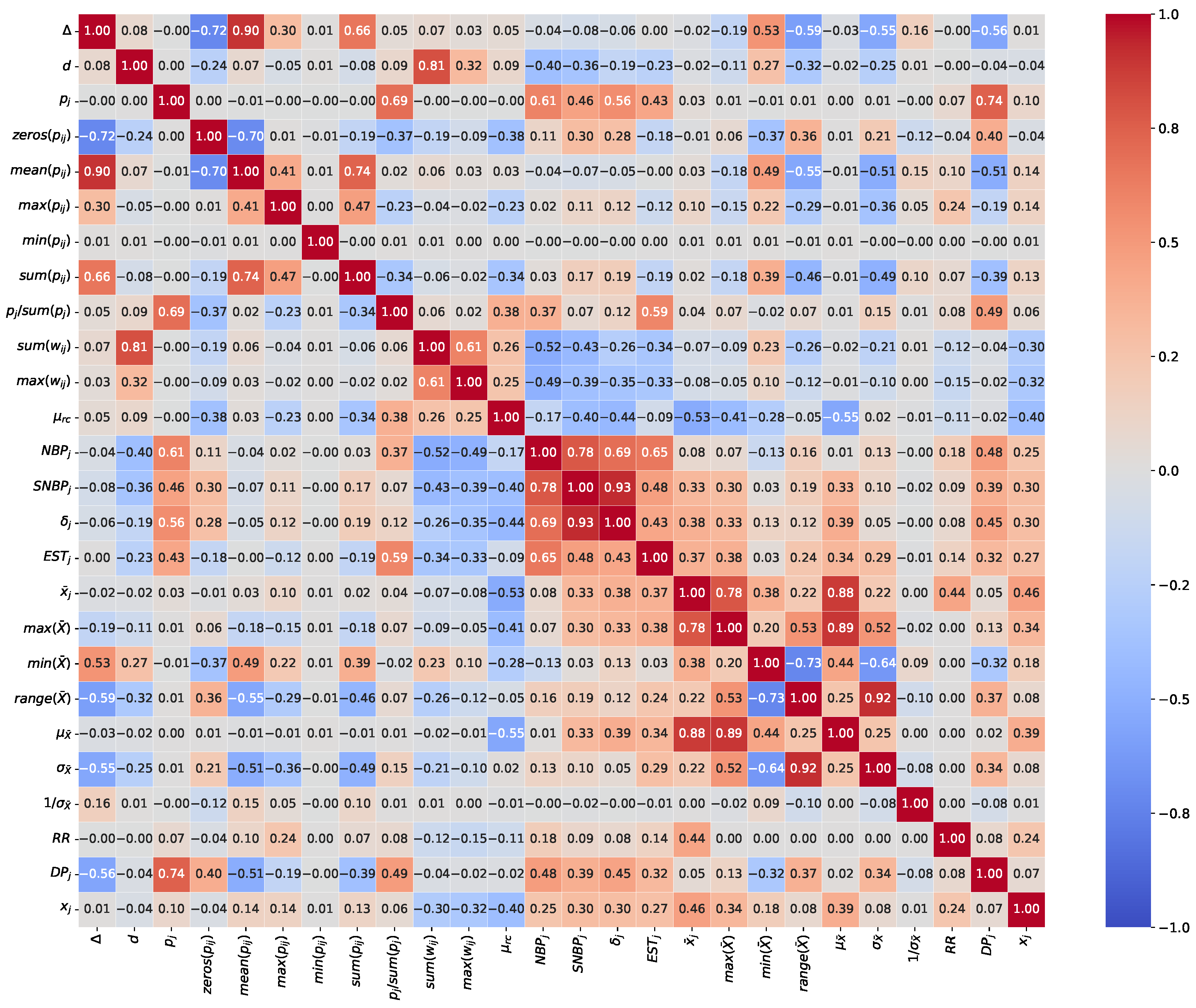
A correlation matrix was computed to identify potential collinearity among generated features, as shown in Figure 1. The analysis revealed strong correlations between specific feature pairs, most notably:

• $\Delta$ and $\mathrm{mean}\left(p_{ij}\right)$.
• d and $\mathrm{sum}\left(w_{ij}\right)$.
• $SNB{P}_j$ and ${\delta }_j$.
• ${\overline{x}}_j$ and ${\mu }_{\overline{x}}$.
• $\max \left(\overline{X}\right)$ and ${\mu }_{\overline{x}}$.
• $\mathrm{range}\left(\overline{X}\right)$ and ${\sigma }_{\overline{x}}$.

Despite these findings, the decision was made to retain the majority of the feature set. This strategy aims to enable non-linear models, such as a Multi-Layer Perceptron (MLP) or SVMs, to capture complex interactions that might be lost when all correlated variables are strictly eliminated.

The sole exception to this approach was the variable $\min \left(p_{ij}\right)$. Preliminary experimental trials indicated that this attribute, in some cases, slightly reduced performance metrics. Consequently, it was excluded from the final training set.

3.3.2. Transformation and Scaling

Skewed data can affect the performance of some machine learning algorithms, such as logistic regression (LR). To mitigate the impact of data asymmetry and facilitate the learning process, a feature-specific transformation strategy was implemented. An analysis of the input variables revealed different degrees of skewness; therefore, distinct transformations were applied, depending on the distributional characteristics of each feature. A natural logarithm was applied to variables exhibiting extreme positive skewness, specifically $SNB{P}_j$ and ${\delta }_j$. Similarly, the Box–Cox transformation was utilized for $NB{P}_j$ and $ES{T}_j$. Finally, a square root transformation was employed for features showing moderate skewness, such as $D{P}_j$, ${\mu }_{rc}$ and $p_j/\mathrm{sum}\left(p_j\right)$.

Following these adjustments, a feature-scaling technique was applied to standardize the variables. This step ensures that all features contribute equally to the model training process, preventing attributes with larger magnitudes from dominating the objective function.

3.3.3. Final Dataset Composition

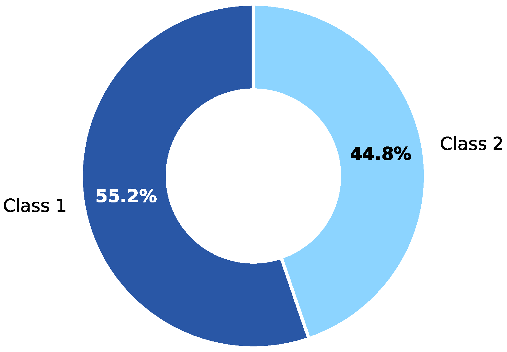
The final data set comprises 435 instances, totaling 18,600 items, of which 10,273 items belong to class 1 (items included in the solution) and 8327 to class 0 (excluded items). Figure 2 illustrates the proportion of both classes. Since they are essentially balanced, no resampling techniques were necessary to address class imbalance.

3.4. Model Training and Selection

Model training is the fundamental process of learning patterns from data by optimizing an algorithm’s internal parameters to minimize an error function, which quantifies the discrepancy between the model’s predictions and the actual target values. The ultimate objective of this phase is generalization, the ability of the model to accurately predict outcomes on unseen instances effectively [7].

Given the combinatorial complexity of the QMdKP, it was not possible to assume a priori the nature of the relationship between instance features and optimal solutions. Therefore, a diverse battery of twelve predictive models spanning multiple learning paradigms was evaluated, with the aim of empirically determining which approach best characterizes the underlying patterns in the data.

The selected models are defined as follows:

• Logistic Regression (LR): a linear model that estimates the probability of class membership using the logistic function to map the output between 0 and 1 [46].
• Gaussian Naive Bayes (GNB): a probabilistic classifier that assumes the features of each class follow a Gaussian distribution. It estimates the required parameters independently for each feature [45].
• Decision Tree (DT): a model that classifies data through a hierarchy of conditional rules, represented visually as a tree structure with decision nodes and leaves [45].
• Random Forest (RF): An ensemble method composed of multiple decision trees. For classification, it employs a “soft voting” strategy, determining the final prediction by averaging the probabilities calculated by the individual trees [45].
• Gradient Boosting (GB): a sequential ensemble technique that builds shallow trees, with which each new model is trained specifically to correct the residual errors of the previous ones [45].
• AdaBoost (AB): an adaptive ensemble algorithm that trains weak learners sequentially, assigning higher weights to instances misclassified by previous models to focus training on difficult cases [7].
• XGBoost: an open-source software library that provides an optimized, distributed, and scalable implementation of the gradient boosting framework [47].
• LightGBM: a gradient boosting framework that uses tree-based learning algorithms, designed specifically for efficient training on large-scale datasets [48].
• CatBoost: a gradient boosting library that implements a specialized algorithm to handle categorical features automatically and uses an ordered boosting scheme to reduce overfitting [49].
• K-Nearest Neighbors (k-NN): an instance-based algorithm that classifies a new data point by finding its k nearest neighbors in the training set and assigning the most common class among them [45].
• Support Vector Machine (SVM): a classification algorithm that uses kernel functions to map data into a higher-dimensional feature space, where it seeks the hyperplane that maximizes the margin between classes [45].
• Multi-Layer Perceptron (MLP): a neural network architecture consisting of an input layer, one or more hidden layers, and an output layer, capable of modeling complex non-linear relationships [7].

These particular algorithms were selected to assess distinct structural approaches. LR was established as a performance baseline, offering high computational efficiency and interpretability [45]. To address the limitations of single estimators, ensemble methods were included; specifically, RF was selected for its robustness against overfitting [45]. Furthermore, the boosting family represented by AB, GB, and optimized implementations such as XGBoost, LightGBM, and CatBoost was incorporated due to its capability to sequentially correct residual errors [7]. Finally, algorithms capable of modeling complex non-linear decision boundaries were essential. This category includes SVM and MLP, which allow the capture of intricate patterns that linear or shallow learners might overlook.

3.4.1. Machine Learning Hyperparameters

Regarding model configuration, we adopted the default settings provided via the standard libraries. This decision was made to ensure a fair baseline assessment of the intrinsic capabilities of each classifier, avoiding the bias that could be introduced through unequal optimization efforts across different algorithms. The specific hyperparameters utilized for each model are detailed in

Table 2. Hyperparameter configuration for the evaluated models.

Algorithm	Parameters
LR	penalty = l2, $C=1.0$, solver = lbfgs
GNB	(No hyperparameters)
DT	criterion = gini, splitter = best
RF	n_estimators = 100, criterion = gini, max_depth = None, max_features = sqrt
GB	n_estimators = 100, learning_rate = 0.1, max_depth = 3
AB	n_estimators = 50, learning_rate = 1.0
XGBoost	eval_metric = logloss, use_label_encoder = False
LightGBM	boosting_type = gbdt, n_estimators = 100
CatBoost	iterations = 1000
k-NN	n_neighbors = 5, metric = minkowski
SVM	kernel = rbf, $C=1.0$, gamma = scale
MLP	max_iter = 1000, hidden_layer_sizes = (100,), activation = relu

Note: Values correspond to the standard default implementations provided via the scikit-learn library. These parameters were maintained fixed to establish a consistent baseline for comparative analysis.

.

Finally, to assess the generalization capability of the classifiers, the dataset was randomly partitioned into a training set (80%) and a testing set (20%). A fixed random seed was employed across all procedures to ensure the reproducibility of the experiments. All models were fitted exclusively on the training partition to prevent data leakage, ensuring an unbiased evaluation on unseen instances.

3.4.2. Model Evaluation

Following the training phase, we validated the predictive capability of the suite of models configured on the testing set. The goal of this evaluation was to identify the most suitable classifier to integrate into the hybrid solver. To guarantee the complete reproducibility of the analysis, model training utilized a fixed random seed.

Table 3. Comparative Summary of Classifier Performance.

Algorithm	Precision	Recall	F1-Score	Accuracy
LR	0.844	0.861	0.852	0.835
GNB	0.770	0.790	0.780	0.753
DT	0.780	0.779	0.780	0.756
RF	0.822	0.829	0.825	0.806
GB	0.835	0.847	0.841	0.823
AB	0.808	0.822	0.815	0.793
XGBoost	0.849	0.842	0.846	0.830
LightGBM	0.852	0.856	0.854	0.838
CatBoost	0.847	0.854	0.851	0.834
k-NN	0.810	0.815	0.813	0.792
SVM	0.858	0.850	0.854	0.839
MLP	0.867	0.833	0.850	0.837

summarizes the performance metrics obtained, including precision, recall, F1-score, and accuracy.

As observed, the results reflect a scenario of high competitiveness among the tested classifiers, with several models showing performance above $80\%$. The F1-Score performance is narrowly led by the SVM and LightGBM models, both achieving $85.4\%$. Regarding precision, MLP leads with $86.7\%$, followed by SVM at $85.8\%$. In terms of recall, the performance is led by LR and LightGBM at $86.1\%$ and $85.6\%$, respectively. Furthermore, SVM achieves the best accuracy with $83.9\%$, closely followed by LightGBM at $83.8\%$.

Although specific algorithms exhibit slightly superior performance in either precision or recall, these improvements are achieved at the expense of the opposing metric. For instance, while the MLP model reaches the highest precision in the suite ($86.7\%$), it does so with a notable drop in recall ($83.3\%$).

Therefore, despite the narrow margins across performance metrics, the SVM is selected for the hybrid optimization framework. Its selection is justified by its ability to maintain a robust equilibrium, combining high precision ($85.8\%$) with strong recall ($85.0\%$), which is essential for the reliability of the solver.

4. Hybrid Solving Approach

The proposed hybrid strategy integrates the predictive model with the exact solver, utilizing the former not as a substitute but as an intelligent filter. Specifically, the ML algorithm is employed to reduce the size of the problem, effectively defining a condensed subproblem for subsequent resolution by the exact optimizer. The descriptions of the variables and parameters are presented in

Table 4. Summary of notation used in the Hybrid-Exact Approach.

Symbol	Description
${\widehat{p}}_j$	predicted probability of item j belonging to the optimal solution
${\tau }_{low}$	lower probability threshold for fixing variables to 0
${\tau }_{high}$	upper probability threshold for fixing variables to 1
${\mathcal{J}}_0$	set of items fixed to 0 (discarded)
${\mathcal{J}}_1$	set of items fixed to 1 (included)
${\mathcal{J}}_{free}$	set of free variables to be optimized by the exact solver

.

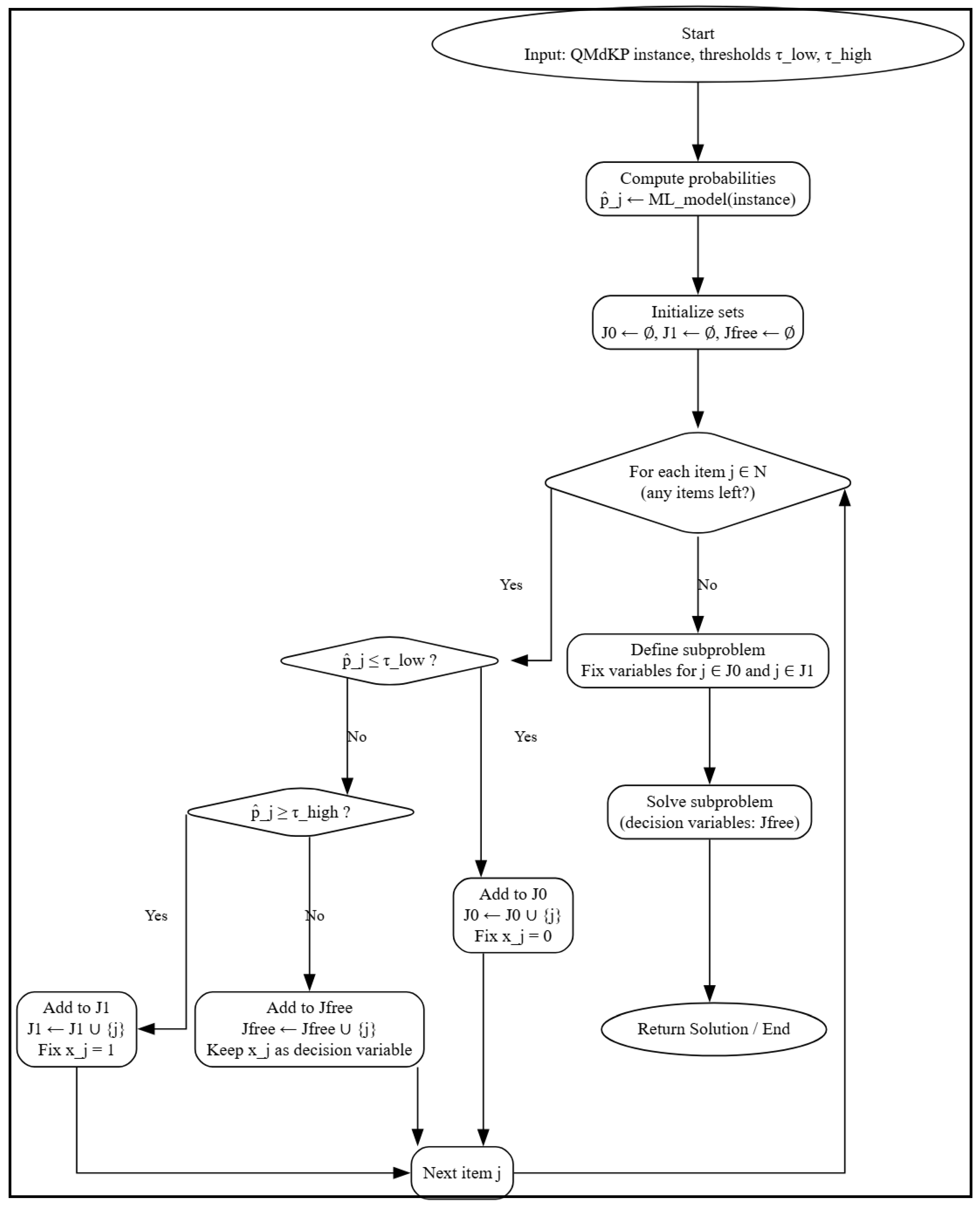
The workflow of the proposed variable reduction mechanism is illustrated in Figure 3. Given a new instance, we compute the corresponding feature vectors and apply the same normalization and preprocessing steps used during training, ensuring that the inference data remain consistent with the model’s input representation. A detailed explanation of the procedure, together with its Algorithm 1, is provided later in this section.

The predictive model then generates a continuous probability score ${\widehat{p}}_j\in [0, 1]$ for each item j, quantifying the likelihood of its inclusion in the optimal solution. Instead of applying a direct binary classification (which uses a default threshold of 0.5), we establish a conservative decision rule defined by a lower threshold, ${\tau }_{low}=0.05$, and an upper threshold, ${\tau }_{high}=0.95$. Based on these confidence levels, the decision variables $x_j$ are partitioned into three sets. First, the set ${\mathcal{J}}_0$ comprises items where ${\widehat{p}}_j\le {\tau }_{low}$; these are deemed irrelevant and fixed to zero ($x_j=0$). Conversely, the set ${\mathcal{J}}_1$ includes items with ${\widehat{p}}_j\ge {\tau }_{high}$, which are fixed to one ($x_j=1$). Finally, items falling within the uncertainty interval form the set ${\mathcal{J}}_{free}$, remaining as free variables.

Algorithm 1 Solution Space Reduction Mechanism

Require: QMdKP instance, thresholds ${\tau }_{low}$, ${\tau }_{high}$ Ensure: Solution   1: Get probabilities ${\widehat{p}}_j\leftarrow$ ML_model$\left(\mathrm{QMdKP}\mathrm{instance}\right)$   2: for each item $j\in N$ do   3:        if ${\widehat{p}}_j\le {\tau }_{low}$ then   4:             ${\mathcal{J}}_0\leftarrow {\mathcal{J}}_0\cup \left\{j\right\}$                                                                                                          ▷ Fix $x_j=0$   5:        else if ${\widehat{p}}_j\ge {\tau }_{high}$ then   6:             ${\mathcal{J}}_1\leftarrow {\mathcal{J}}_1\cup \left\{j\right\}$                                                                                                          ▷ Fix $x_j=1$   7:        else   8:             ${\mathcal{J}}_{free}\leftarrow {\mathcal{J}}_{free}\cup \left\{j\right\}$                                                                  ▷ Keep $x_j$ as a decision variable   9:        end if 10: end for 11: Define a subproblem using fixed variables from ${\mathcal{J}}_0$ and ${\mathcal{J}}_1$ 12: Solve the subproblem for ${\mathcal{J}}_{free}$ 13: return Solution

Following the variable fixation, the optimization scope is restricted exclusively to ${\mathcal{J}}_{free}$. The exact solver is invoked to determine the optimal values for these remaining items, while the variables belonging to ${\mathcal{J}}_0$ and ${\mathcal{J}}_1$ are treated as constants.

The resulting reduced subproblem is formulated as follows:

$$\begin{array}{cc}\hfill \mathrm{maximize}Z=& \sum _{j=1}^n{p}_j{x}_j+\sum _{j=1}^{n-1}\sum _{k=j+1}^n{p}_{jk}{x}_j{x}_k\hfill \end{array}$$

(11)

$$\begin{array}{cc}\hfill \mathrm{subject}\mathrm{to}& \sum _{j=1}^n{w}_{ij}{x}_j\le C_i,\forall i=1,\dots ,d\hfill \end{array}$$

(12)

$$\begin{array}{cc}\hfill & x_j=0,\forall j\in {\mathcal{J}}_0\hfill \end{array}$$

(13)

$$\begin{array}{cc}\hfill & x_j=1,\forall j\in {\mathcal{J}}_1\hfill \end{array}$$

(14)

$$\begin{array}{cc}\hfill & \hspace{0.17em}{x}_j\in \{0,1\},\forall j\in {\mathcal{J}}_{free}\hfill \end{array}$$

(15)

Equations (13) and (14) serve as the mechanism for dimensionality reduction. In fact, by pre-assigning values to high-confidence items, the dimensionality of the optimization problem decreases from n to $|{\mathcal{J}}_{free}|$. Given that the computational complexity of exact algorithms, such as Branch-and-Bound, is primarily driven by the number of binary decisions required to build the search tree, this mechanism is designed to prune the combinatorial space significantly. Consequently, the solver is relieved from evaluating trivial branches, allowing it to focus its resources exclusively on the most uncertain items (${\mathcal{J}}_{free}$).

It is important to emphasize that this strategy does not replace the exact solver with a predicted approximation. Instead, the ML model functions as a pre-processing filter that enhances the solver’s efficiency. By identifying potentially trivial decisions (variables in ${\mathcal{J}}_0$ and ${\mathcal{J}}_1$), the mechanism allows the optimizer to focus its computational efforts solely on the complex, uncertain region of the search space, thereby extending its applicability to larger instances that would otherwise be computationally prohibitive.

5. Metaheuristic Approach

While the hybrid framework aims to accomplish optimality by reducing the search space, large-scale instances of the QMdKP often remain computationally prohibitive for exact methods due to their NP-hard nature. To address this scalability issue, we propose a metaheuristic approach designed to find high-quality solutions within limited time windows. The algorithm integrates an ML-guided initialization that allows bypassing the initial exploration phase, focusing on refining an already promising feasible solution. Additionally, a first-improvement strategy is incorporated to avoid the burden of exhaustive neighborhood evaluation.

The core algorithm is based on an iterated local search (ILS) architecture, a method chosen for its proven ability to balance intensification (local search) and diversification (perturbation) in combinatorial optimization problems [50]. The ML-based construction strategy is compared against a standard randomized heuristic to measure the impact of the predictive model in finding high-quality initial solutions. The metaheuristic variables are shown in

Table 5. Summary of notation used in the problem formulation and the proposed framework.

Symbol	Description
$S_0$	initial feasible solution for the metaheuristic
S	current solution
$S_{best}$	best solution found throughout the search
$\delta$	marginal contribution of an item to the objective function
$patience$	counter of consecutive non-improving iterations
$T_{low}$	lower threshold of iterations defining the first perturbation phase
$T_{high}$	upper threshold of iterations triggering the strong perturbation phase

.

The first stage of the ILS is the construction of an initial feasible solution, $S_0$. We implement two distinct strategies. The first one is a deterministic approach that is guided by the machine-learning model and used only to generate the starting solution. Starting with an empty knapsack, items are then sorted in descending order, based on their SVM probability score, ${\widehat{p}}_j$. The algorithm then scans this ranked list and attempts to insert each item (setting $x_j=1$) into the solution; if adding an item would violate any knapsack capacity constraint, the item is skipped, ensuring feasibility throughout the construction.

In contrast to the deterministic ML-based approach, which relies strictly on the probabilities predicted by the model, we establish a performance baseline using a randomized construction driven by a heuristic score. This strategy adopts the principles of the Greedy Randomized Adaptive Search Procedure (GRASP), which builds a solution iteratively by combining a greedy criterion with a stochastic selection mechanism. Unlike the previous strategy, this method avoids local optima during the construction phase by selecting a random item from a restricted candidate list (RCL) of high-quality elements, rather than always choosing the absolute best one [51].

In the absence of predictive guidance, the potential contribution of an item to the objective function is estimated via a score, $h_j$, defined as the ratio between its aggregate profit (linear and quadratic) and its average resource consumption:

$$h_j={\displaystyle \frac{p_j+{\sum }_{k\ne j}{p}_{jk}}{\frac{1}{d}{\sum }_{i=1}^d{w}_{ij}}}.$$

(16)

Based on this score, the algorithm builds the RCL with the top $\beta$ items (configured with $\beta =0.3$) and selects one randomly to attempt insertion. This ensures that different execution threads explore diverse regions of the solution space.

Upon establishing the initial solution, $S_0$, the algorithm transitions to an improvement phase based on the Variable Neighborhood Descent (VND) framework [52]. This approach relies on the principle that a local optimum with respect to one neighborhood is not necessarily a local optimum for another. Consequently, the algorithm systematically alternates between two search operators to navigate the solution space in depth.

First, a swap operator is applied. This mechanism attempts to improve the current solution by simultaneously removing a randomly selected item, i, and inserting a non-selected, also random item, j. A move is executed strictly if the swap maintains feasibility with respect to all constraints and yields an increase in the objective function’s value. This operation is particularly effective for navigating the search space without significantly altering the total resource consumption, allowing the replacement of inefficient items with more profitable ones.

Subsequently, an insertion operator is employed. Here, the algorithm iterates through the remaining non-selected items and attempts to activate them ($x_j:0\to 1$) to fill any remaining capacity left after the exchange operations.

To maximize computational speed, the VND follows a first-improvement strategy: candidate moves are scanned in random order, and the first modification that improves the objective value is immediately accepted. The process iterates between these two operators until no further improvements can be found.

When neither the swap nor the insertion operators can find a better solution, the algorithm applies a perturbation mechanism to escape the local optima and explore new regions of the search space. This phase forcibly removes a subset of items from the current solution ($x_j:1\to 0$). The intensity of this perturbation follows a progressive scheme, governed by a patience counter that tracks consecutive non-improving iterations and two thresholds, $T_{low}$ and $T_{high}$, that separate the stagnation phases.

Initially, when the counter value remains below $T_{low}$, the mechanism applies a minimal perturbation by removing the item with the lowest marginal contribution to the total profit ($\delta$). If the search remains trapped ($T_{low}\le patience<T_{high}$), the perturbation strength increases, removing a small random set of items. Finally, if the counter exceeds $T_{high}$, a larger proportional subset is dropped (up to a 15% of the active variables) to force a strong diversification.

Following the perturbation, the algorithm restarts the VND phase from the new partial solution. This cycle of local search and perturbation repeats until a maximum iteration count is reached. The complete workflow of the proposed metaheuristic is summarized in Algorithm 2.

Algorithm 2 Proposed metaheuristic

Input: Initial solution $S_0$, $MaxIter$, thresholds $T_{low},T_{high}$ Output: Best solution $S_{best}$   1: $S\leftarrow S_0;$$S_{best}\leftarrow S_0;$$patience\leftarrow 0;$$iterations\leftarrow 0$   2: while $iterations<MaxIter$ do   3:       repeat   4:             $S\leftarrow$Swap(S)   5:             $S\leftarrow$Add(S)   6:       until no further improvement   7:       if $f\left(S\right)>f\left(S_{best}\right)$ then   8:             $S_{best}\leftarrow S$   9:             $patience\leftarrow 0$ 10:       else 11:             $patience\leftarrow patience+1$ 12:       end if 13:       if $patience<T_{low}$ then 14:             $S\leftarrow$Drop(S, lowest $\delta$) 15:       else if $patience<T_{high}$ then 16:             $S\leftarrow$Drop(S, small random set) 17:       else 18:             $S\leftarrow$Drop(S, 15% of items) 19:       end if 20:       $iterations\leftarrow iterations+1$ 21: end while 22: return $S_{best}$

6. Results and Discussion

6.1. Experimental Setup

All computational experiments were performed on a Linux-based server (Ubuntu 22.04.4 LTS) equipped with an Intel Core i7-5820K CPU @ 3.30GHz and 46 GB of RAM. The algorithms were coded in Python 3.10.12, using Gurobi 12.0.3 as the general-purpose solver. The experiments were run in a serial manner to avoid bias in CPU time measurements caused by parallel execution. Standard data science libraries were used for the machine learning components: pandas, numpy, scikit-learn, matplotlib, seaborn, and joblib.

The experimental evaluation was conducted on an independent validation dataset, generated as described in Section 3.2. The analysis is structured into three main phases. First, in Section 6.2, we evaluate the computational time reduction on medium-sized instances ($n\in \{20, 40, 60, 80\}$), comparing the proposed framework against the standard exact solver. The evaluation begins at $n=20$ because smaller instances (e.g., $n=10$) are computationally trivial for state-of-the-art solvers. Thus, the selected range of instance sizes allows for the observation of the exponential growth of the solving time, avoiding redundant sampling through an increment of 20. Second, in Section 6.3, we assess the solution quality on larger-scale instances ($n\in \{100, 120\}$), for which exact methods become computationally prohibitive. Finally, in Section 6.4, the statistical significance of the performance differences is evaluated.

To quantify the performance improvements, we defined three specific metrics:

• Variable reduction rate ($VR$): The percentage of decision variables fixed by the ML model before the exact solver is entered.

  $$VR={\displaystyle \frac{|S_{\mathrm{fixed}}|}{n}}\times 100$$

  (17)

  where $|S_{\mathrm{fixed}}|$ is the number of variables fixed (either to 0 or 1).
• Relative time improvement ($\Delta T$): This value quantifies the percentage variation in the computational time required by the proposed ML method ($T_{ML}$) (Hybrid Solver or ML-based Metaheuristic) with respect to the baseline reference ($T_{base}$). $T_{ML}$ accounts for the entire predictive process, including preprocessing and inference.

  $$\Delta T(\%)={\displaystyle \frac{T_{base}-T_{ML}}{T_{base}}}\times 100$$

  (18)
• Gap ($\Delta Z$): The relative difference in the objective function value between the baseline solution ($Z_{base}$) and the proposed ML method’s solution ($Z_{ML}$), defined as:

  $$\Delta Z(\%)={\displaystyle \frac{Z_{base}-Z_{ML}}{Z_{base}}}\times 100$$

  (19)
  Since the QMdKP is a maximization problem, a negative gap value indicates that the proposed method achieved a better solution than the baseline.

6.2. Hybrid Approach Performance

To evaluate the impact of the proposed hybrid framework, we compared its performance against the standard exact solver. The experiments were conducted on the validation set of 540 instances, categorized by problem size (n).

Table 6. Performance summary: hybrid vs. exact method.

Size	Exact	Hybrid	Var.	Time	Gap
($\mathit{n}$)	Time (s)	Time (s)	Red. ($\mathit{V}\mathit{R}$)	Imp. ($\mathbf{\Delta }\mathit{T}$)	($\mathbf{\Delta }\mathit{Z}$)
20	0.11	0.28	21.56%	−278.90%	0.51%
40	2.18	0.56	33.59%	20.05%	0.26%
60	120.32	5.33	34.94%	71.38%	0.14%
80	1555.66	110.08	31.45%	83.00%	0.01%

summarizes the average results obtained for each instance size according to the metrics defined earlier.

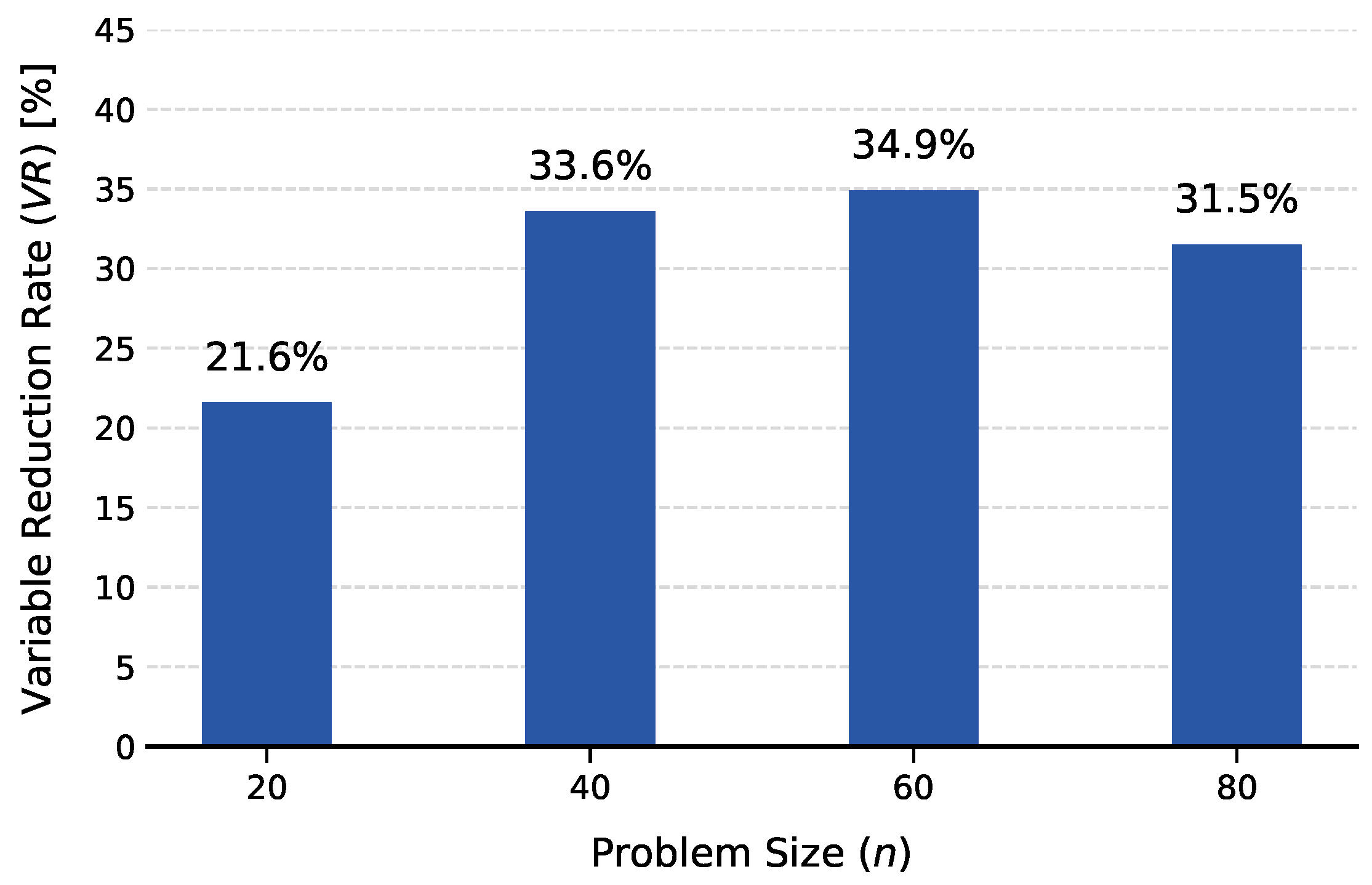
As illustrated in Figure 4, the variable fixation mechanism demonstrates robust behavior. While the reduction rate ($VR$) is more conservative for small instances ($21.6\%$ for $n=20$), it stabilizes between $31\%$ and $35\%$ for instances of size $n\ge 40$. This indicates that the predictive capability of the classifier does not degrade as the combinatorial complexity increases; rather, it consistently identifies and fixes approximately one-third of the search space, regardless of the problem dimension.

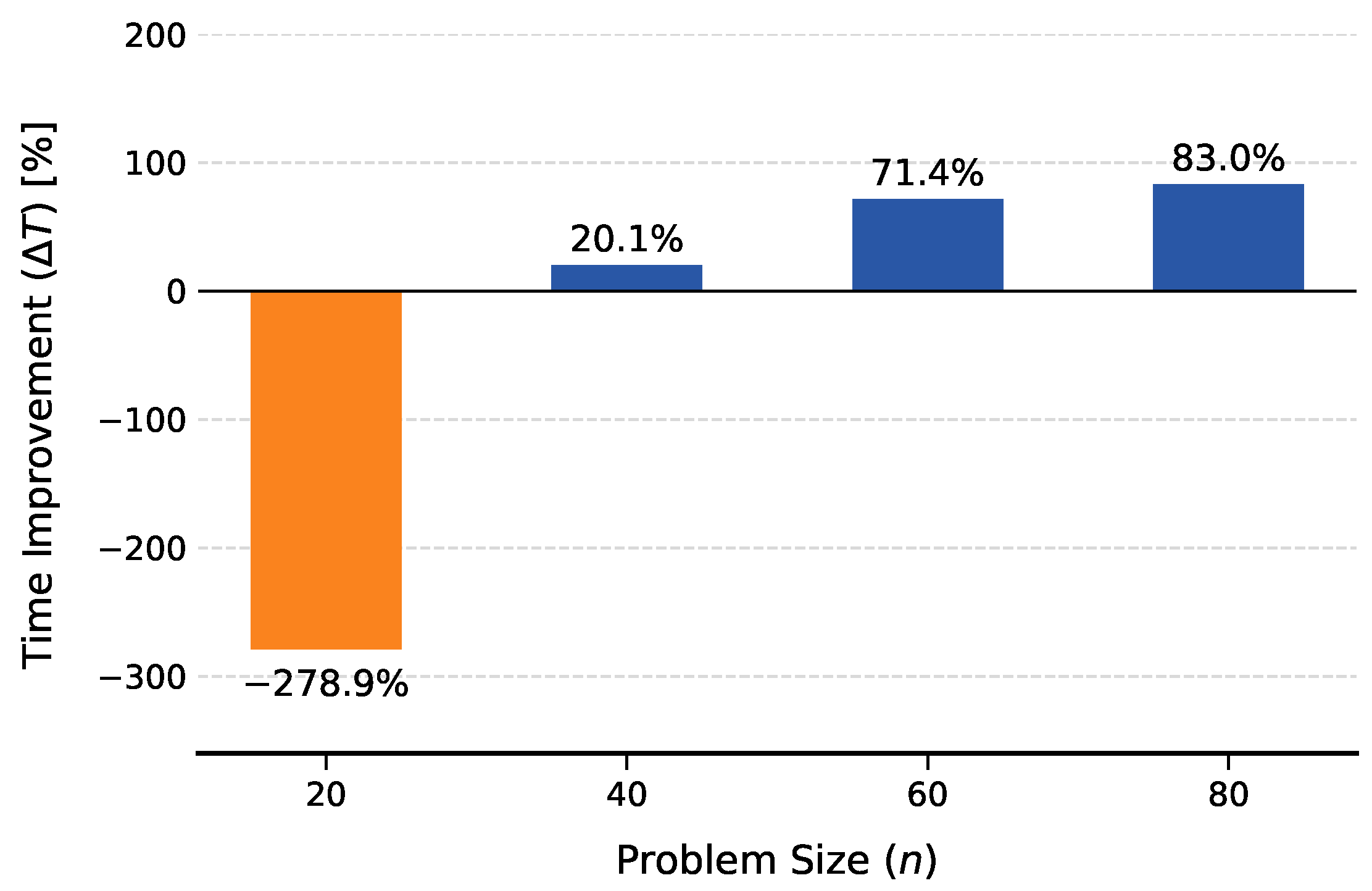
Figure 5 illustrates the relative time improvement ($\Delta T$) achieved across different instance sizes. For small instances ($n=20$), the hybrid approach exhibits a negative performance ($\Delta T=-278.9\%$), implying that the overhead of feature extraction and ML prediction outweighs the solving time for trivial problems. However, a crossover occurs at $n=40$; where the method achieves a $20.1\%$ improvement. This gain scales dramatically for larger instances, reaching a time reduction of 83.0% for $n=80$. This trend confirms the scalability of the hybrid framework: while the runtime of exact solvers grows exponentially with size, the proposed method leverages variable reduction to maintain tractability.

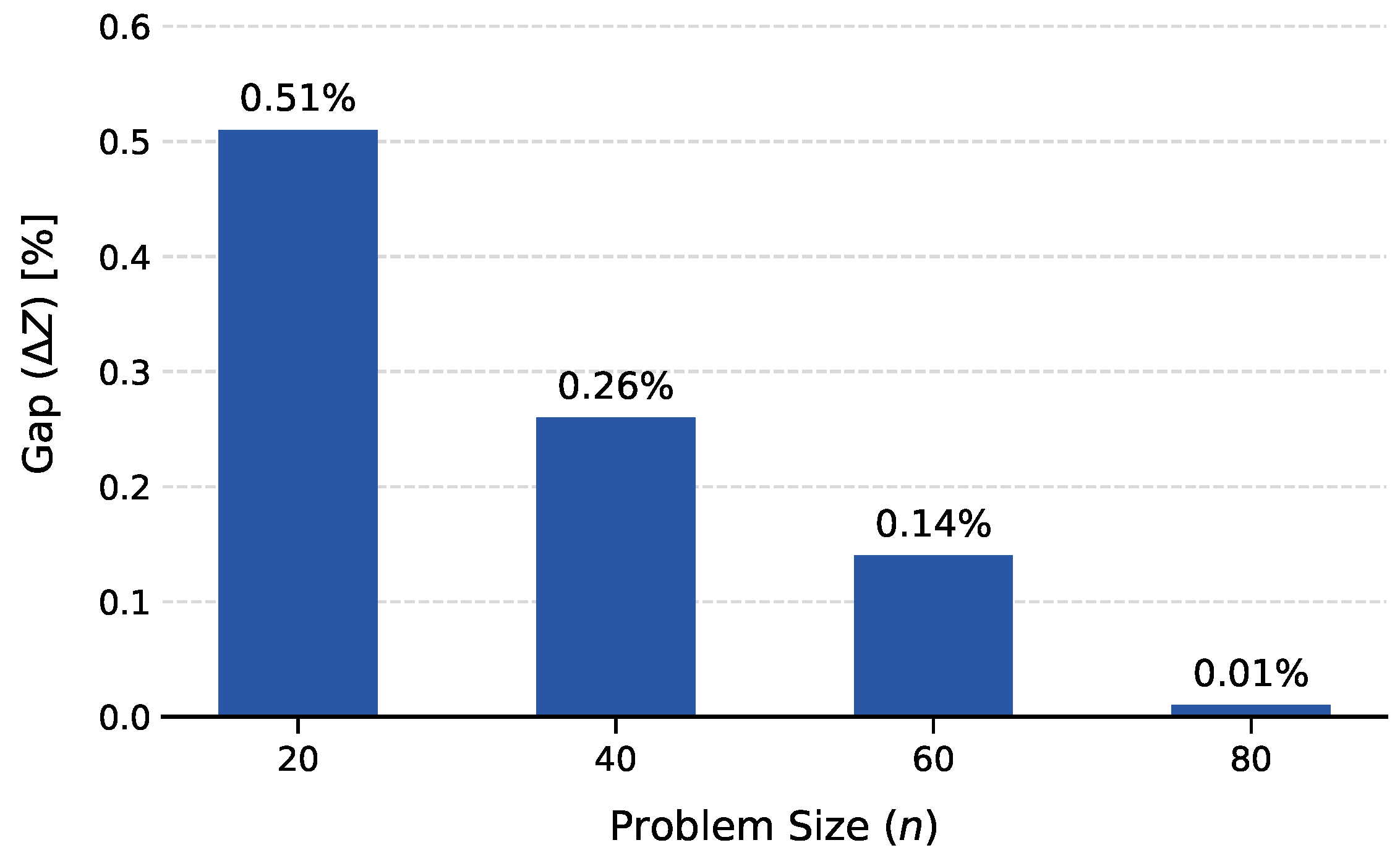
Notably, these efficiency gains are not obtained to the detriment of solution quality. Figure 6 shows an inverse relationship between problem complexity and the optimally gap ($\Delta Z$). The maximum gap observed is marginal ($0.51\%$ for $n=20$) and decreases to a virtually negligible 0.01% for $n=80$. This suggests that, in large-scale problems, the classifier effectively discriminates critical items, preserving the optimal structure within the reduced subproblem.

Overall, the hybrid method yields substantial reductions in computational time for medium-sized instances (40-80 variables) while maintaining competitive solution quality.

6.3. Metaheuristic Approach Performance

In this second phase of the analysis, we assess the efficacy of the proposed metaheuristic by conducting experiments on a validation set of 270 large-scale instances. Since exact methods are computationally prohibitive for these dimensions, the analysis focuses on two key aspects: the impact of the initialization strategy and the overall performance of the proposed algorithm.

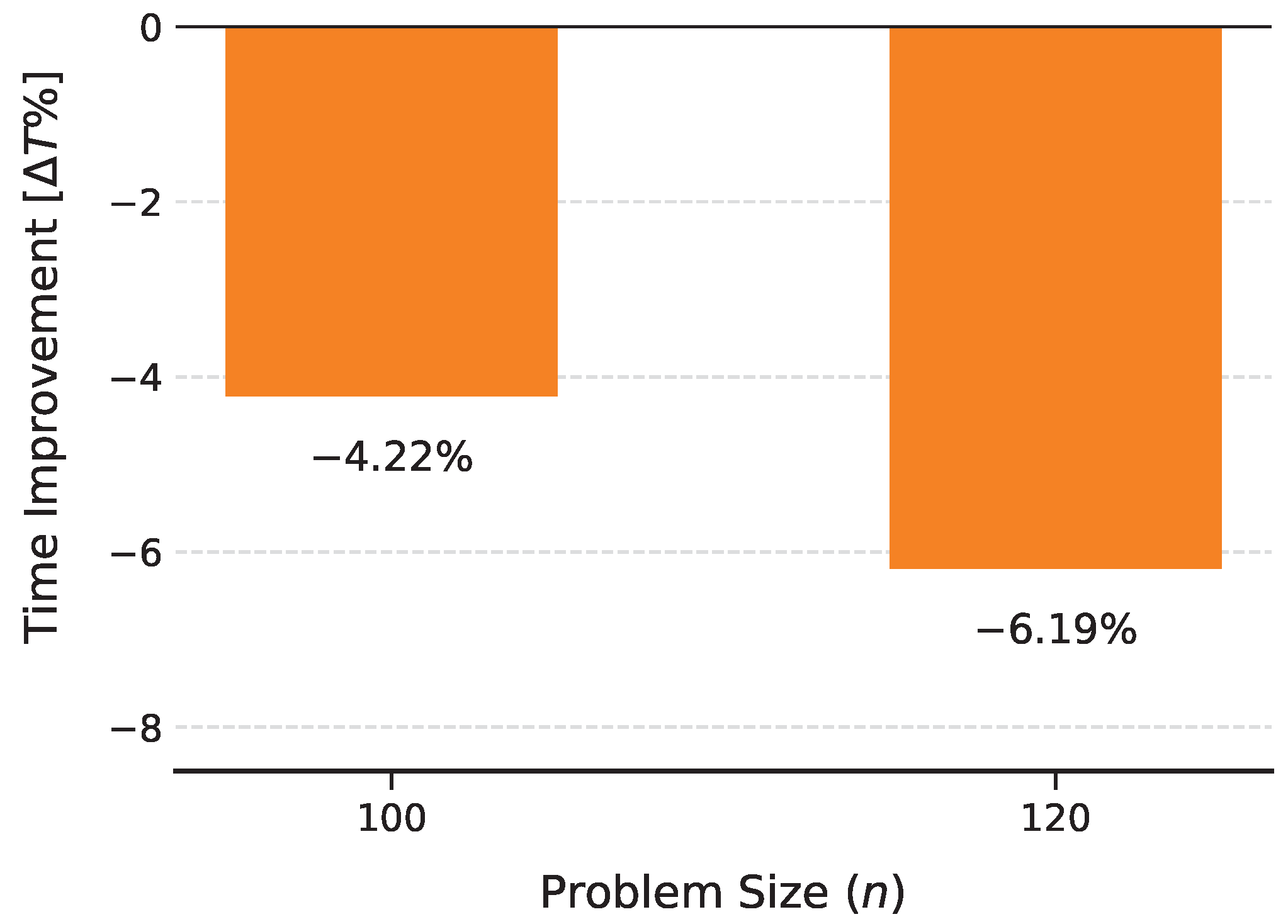
We first tackle the construction method for the initial solution ($S_0$) to evaluate the contribution of the machine learning model compared to the standard GRASP-based heuristic. Specifically, we measure the quality of the $S_0$ and the computational time required to generate it.

Table 7. Comparative summary between the baseline and the ML-based strategy.

Size	Average Time (s)		Time Imp.	Gap
($\mathit{n}$)	Baseline	ML-Based	(%)	(%)
100	4.16	4.19	−4.22	−0.28
120	5.65	5.88	−6.19	−0.40

presents the average metrics obtained for instances of 100 and 120 variables.

Figure 7 illustrates the time difference achieved through the predictive approach relative to the baseline. As observed, the negative values indicate that the ML-based construction incurs a computational overhead, meaning the standard heuristic generates a feasible solution faster than the predictive one. This behavior is expected, as the time measurement accounts for the data preprocessing, feature extraction and prediction stages required by the ML pipeline.

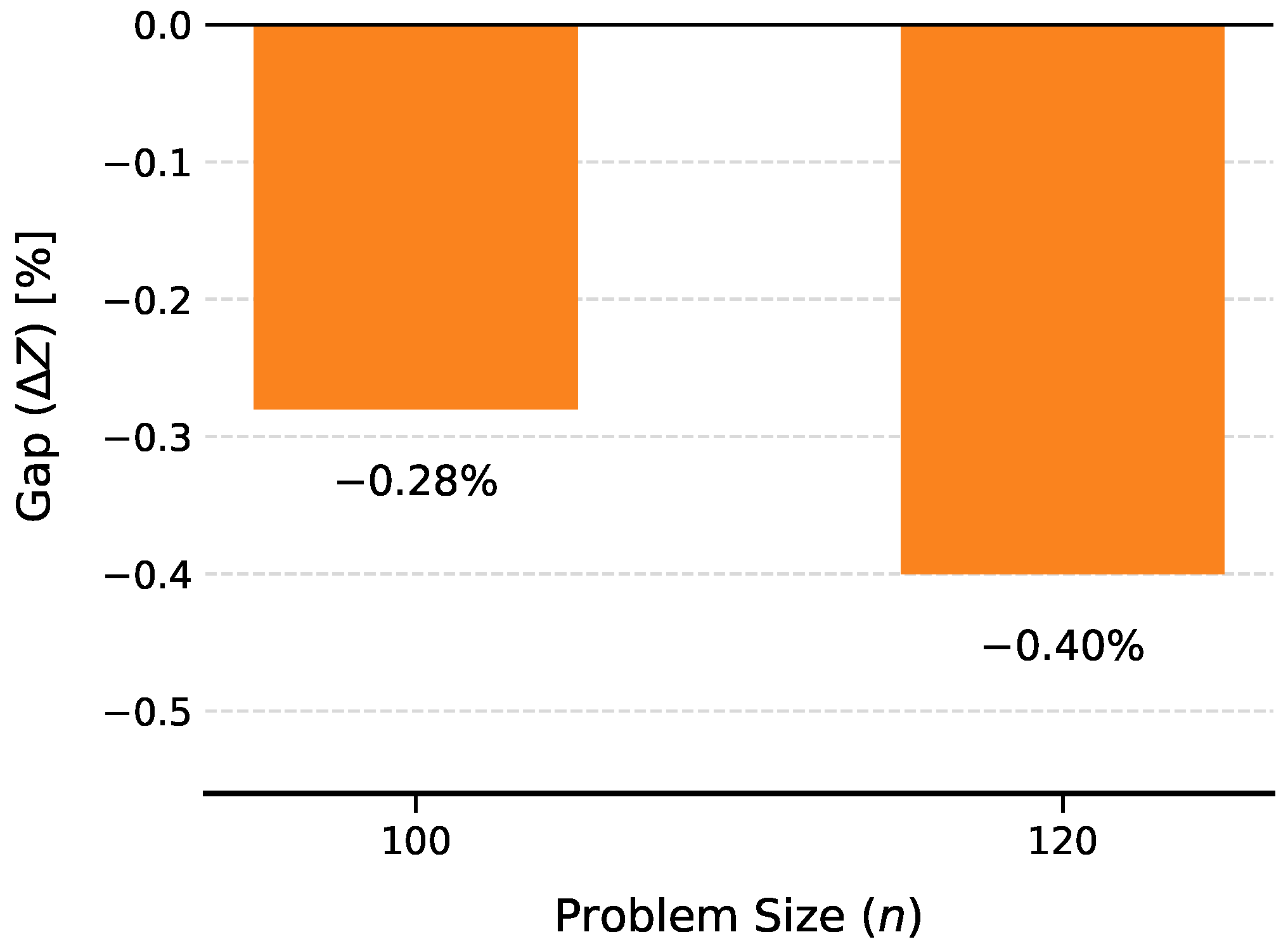
Regarding solution quality, Figure 8 illustrates the average gap of the ML-based solutions relative to the baseline. The consistently negative values across all instances indicate that the ML model provides a superior starting point for the subsequent local search phase. This suggests that the patterns learned by the classifier effectively capture the structural characteristics of high-quality solutions, outperforming the standard greedy criteria based on average weights.

Consequently, the ML-based initialization is selected as the preferred strategy for the proposed metaheuristic. Although this approach incurs a slight computational overhead due to the preprocessing stage (less than 3 s on average), this cost is negligible when contrasted with the amount of time required by exact methods. This trade-off is justified because a superior starting point directs the subsequent local search toward more promising regions of the solution space, increasing the likelihood of reaching high-quality solutions.

Comparison with the Hybrid Solver

Having established the configuration of the metaheuristic, we proceed to compare its performance against the Hybrid Solver on the same set of large-scale instances. This analysis focuses on two critical dimensions: computational efficiency and solution stability.

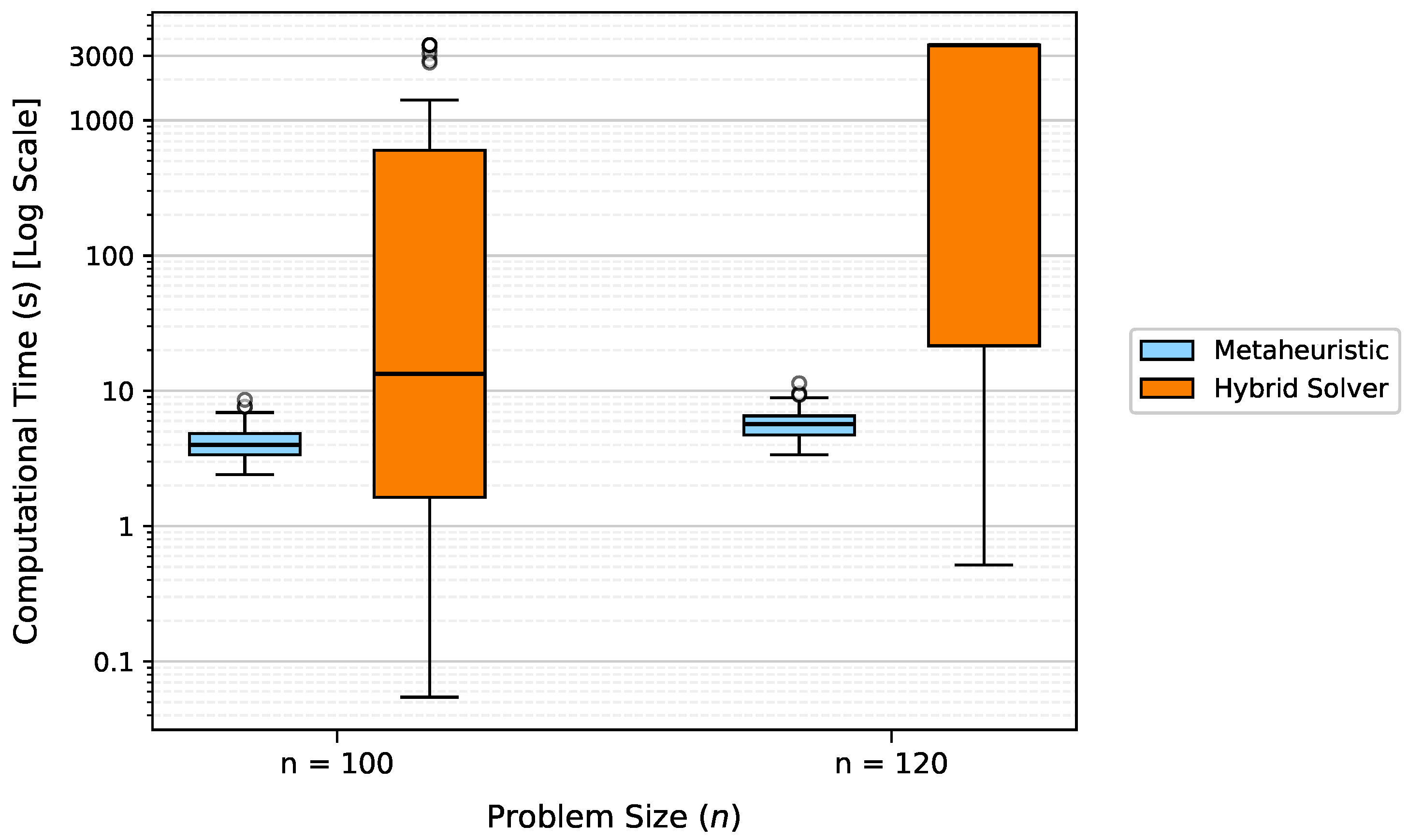
Figure 9 presents the distribution of computational times required for both methods. Note that a logarithmic scale is used on the y-axis to visualize the significant difference in magnitude. The results reveal a noticeable contrast in behavior: while the hybrid solver exhibits high variability, with execution times ranging from a fraction of a second to over 3000 s, the ML-based Metaheuristic demonstrates remarkable robustness. The narrow interquartile range of the proposed method indicates a consistent performance, regardless of the instance complexity. This represents a time reduction of several orders of magnitude compared to the median performance of the hybrid approach.

Table 8. Comparison of computational time and gap between the hybrid solver and the proposed metaheuristic. Note: The gap (%) represents the relative deviation of the metaheuristic with respect to the hybrid solver’s solution.

Size (n)	Average Time (s)		Gap (%)
	Hybrid Solver	Metaheuristic (ML)
100	786.0 ± 1391.5	4.19 ± 1.11	1.74
120	2015.5 ± 1714.2	5.88 ± 1.46	1.85

details the average execution times alongside their standard deviations. As shown, the ML-based strategy requires less than 6 s on average, with a negligible standard deviation that corroborates its stability. In contrast, the hybrid solver presents deviation values that exceed its own mean, confirming its unpredictability. Crucially, the table also addresses the solution quality. Despite the massive reduction in computational time, the ML-based strategy yields solutions with a gap of less than 2% in comparison with the ones found by the hybrid solver. This indicates that the proposed method achieves a highly favorable balance, offering near-optimal solutions in a negligible fraction of the time required by the exact method.

6.4. Statistical Analysis

To rigorously validate the performance differences between the proposed strategies and their respective baseline methods, we conducted a statistical analysis using the Wilcoxon signed-rank test. The significance level was set to $\alpha =0.05$. The results, summarized in

Table 9. Summary of statistical comparisons using the Wilcoxon signed-rank test.

Metric	Size (n)	p-Value	Significance
Hybrid Solver vs. Exact Method
Time	20	1.0000	No
	40	<0.001	Yes
	60	<0.001	Yes
	80	<0.001	Yes
Objective Function	20	<0.001	Yes
	40	<0.001	Yes
	60	<0.001	Yes
	80	0.5192	No
ML Initialization vs. Random Construction
Time	100	0.1822	No
	120	<0.001	Yes
Objective Function	100	<0.001	Yes
	120	<0.001	Yes
ML Metaheuristic vs. Hybrid Solver
Time	100	<0.001	Yes
	120	<0.001	Yes
Objective Function	100	<0.001	Yes
	120	<0.001	Yes

, address three key dimensions of our contribution: the efficiency of the hybrid solver, the impact of the ML initialization, and the scalability of the metaheuristic.

First, we compared the hybrid solver against the exact method on small and medium-sized instances. Regarding computational time, the results show no significant difference for small instances ($n=20$, $p=1.0$), for which the overhead of the ML model offsets the time saved by the problem reduction. However, for $n\in \{40, 60, 80\}$, the hybrid solver becomes significantly faster ($p<0.001$), confirming its ability to accelerate the resolution process. In terms of solution quality, the exact method is statistically superior for $n=20, 40,$ and 60. Remarkably, for the largest instances in this set ($n=80$), the difference in quality becomes statistically non-significant ($p=0.5192$). This suggests that, for this size, the hybrid solver’s solutions are statistically indistinguishable from those of the exact method.

Second, we evaluated both construction approaches for the metaheuristic. The analysis confirms that the ML-based initialization yields significantly better objective function values than the random construction. Regarding computational cost, for $n=100$, the time difference is not statistically significant ($p=0.1822$), indicating that the ML prediction overhead is negligible in this case. However, a significant time difference appears for $n=120$. As we have explained previously, the superior quality of the starting solution justifies this additional computational cost.

Finally, comparing the metaheuristic against the hybrid-exact solver, the tests confirm the significant reduction in computational time. While, as is expected of an exact method, the hybrid solver maintains a statistical advantage in solution quality, the metaheuristic achieves significantly lower execution times.

7. Conclusions

This paper has introduced a framework comprising two distinct solution strategies for the QMdKP. The first strategy employs a variable-fixing mechanism to prune the search space prior to optimization, while the second constructs an initial solution utilizing ML predictions for an iterated local search metaheuristic. First, a comprehensive description of the synthetic data generation process and exploratory analysis is detailed. Subsequently, a variety of ML models are trained on the consolidated dataset and tested on their capability to effectively predict the inclusion of an item to the optimal solution.

Several algorithms, including LR, LightGBM, CatBoost, and SVM, show similar performance across the evaluation metrics, yielding values over 84% for precision, recall, F1-score, and accuracy. The SVM is ultimately selected due to its high F1-score, reflecting well-balanced precision and recall. However, it is worth noting that similar outcomes for the solution strategies could likely have been achieved using the other top-performing models.

Therefore, the performance of the hybrid solver was evaluated against the exact method. Statistical analysis confirms that, while the proposed approach offers no advantage for small instances due to computational overhead, it significantly outperforms the standard solver for medium-sized instances. In fact, the tests revealed that, for $n=80$, the solutions provided by the ML solver are statistically indistinguishable from the optimal ones found by the exact method, achieving an average time reduction of 83%.

Regarding instances with a larger number of items, the ML-guided constructive method is compared against a randomized heuristic. Although the ML-based strategy incurs a slight time cost of approximately 5%, the approach yields significantly superior solution quality, justifying the selection of this one as the initialization method. Finally, the ML metaheuristic is benchmarked against the hybrid-exact solver. The results show that, on average, the metaheuristic maintains a stable execution time of around five seconds, whereas the hybrid solver exhibits significant variability, reaching up to 3400 s in certain cases. This reduction in time was proven to be significant, demonstrating the method’s capability of providing high-quality solutions within limited time windows.

While solution space reduction approaches have been applied to other knapsack problem variants [40], to the best of our knowledge, this work represents the first specific design of ML techniques for the QMdKP. Furthermore, this paper extends the scope of the framework by integrating the predictive model into a metaheuristic, effectively tackling instances where exact methods are computationally prohibitive.

The ML-based variable fixing consistently reduced the decision space by ≈31–35% for $n\ge 40$, yielding average time savings of 20.1% (n = 40), 71.4% (n = 60) and 83.0% (n = 80) with a negligible optimality loss (average gap down to 0.01%). Wilcoxon tests confirm that the time improvements are significant for $n\in \{40, 60, 80\}$ ($p<0.001$) and that, for $n=80$, the objective values are statistically indistinguishable from the exact solver ($p=0.5192$). For large instances, the ML-initialized ILS remains highly stable (4.19 ± 1.11 s for $n=100$, 5.88 ± 1.46 s for $n=120$), while the hybrid solver exhibits large variability (786 ± 1392 s and 2016 ± 1714 s, respectively), achieving solutions within <2% of the hybrid solver.

For future work, we suggest performing hyperparameter tuning to further refine the accuracy of the classifiers. Additionally, future studies should focus on minimizing the computational overhead of the ML component; investigating algorithms with lower inference times could significantly reduce total execution times. Moreover, alternative ML paradigms, such as DRL or graph neural networks, could be explored to tackle this problem. Finally, we propose extending this ML-driven framework to other knapsack problem variants, particularly those involving quadratic profits.