Appendix A
Proof of Lemma 1. We use backward induction to obtain the equilibrium results without the supplier learning effect under no private label encroachment (strategy ON). Given the wholesale price , we can obtain the equilibrium order quantity for the subgame conditional on the wholesale price (i.e., ) from the first-order condition () and the second-order condition (). Anticipating the retailer’s optimal order quantity in the second period, the supplier decides to maximize its profit with the first-order condition () and the second-order condition (), and then, the supplier’s optimal wholesale price is . Based on the above results, we consider the firms’ total optimization problem during two periods, that is, the total profits of the supplier and the retailer are and , respectively. Similarly, based on the wholesale price , we obtain the retailer’s order quantity from the first-order condition and the second-order condition (). Substituting into the expression , we obtain the optimal wholesale price from the first-order condition () and the second-order condition (). Continuing back to the substitution, we further obtain the equilibrium results as shown in Lemma 1. Similarly, simple algebraic calculation leads to the equilibrium results under strategies OF, OS, WN, as shown in Lemmas 2, 3, and 4, respectively. □
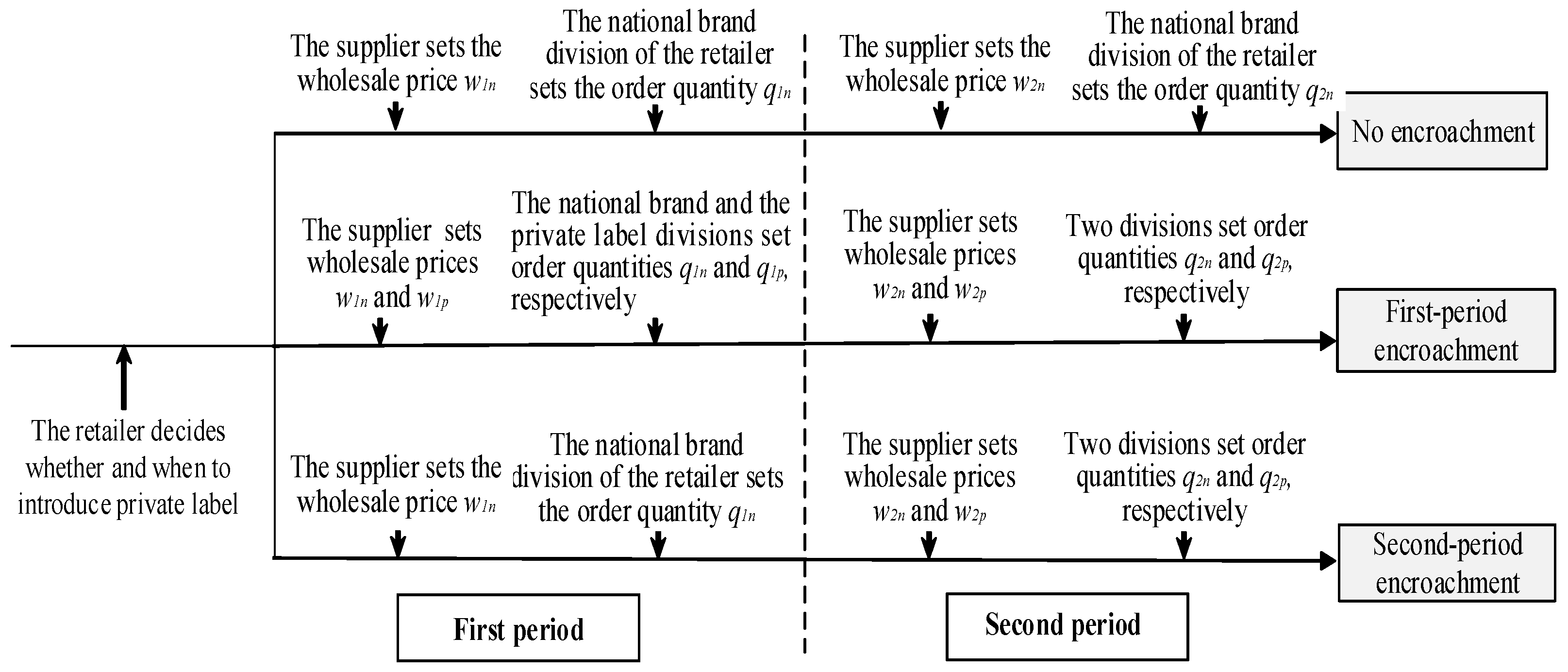
Proof of Lemma 5. In the case where the retailer chooses the first-period encroachment of private labels with the supplier learning effect (strategy WF), we start with the analytical results in the second period. Based on wholesale prices and , order quantities of the retailer’s national brand and private label divisions in the second period are shown as and from first-order conditions ( and ) and second-order conditions ( and ). Anticipating the two divisions’ optimal order quantity in the second period, we further obtain the supplier’s optimal wholesale prices and from first-order conditions ( and ) and the negative semidefinite Hessian matrix (). Based on the above results, we consider the firms’ total optimization problem during two periods. The total profits of the supplier’s and the retailer’s divisions are and , respectively, where and . Similarly, given wholesale prices and , order quantities of the retailer’s divisions in the first period are shown as and from first-order conditions ( and ) and second-order conditions ( and ). Substituting and into , we obtain the optimal wholesale prices from first-order conditions ( and ) and the negative semidefinite Hessian matrix (). Continuing back to the substitution, we further obtain the equilibrium results as shown in Lemma 5. □
Proof of Lemma 6. Similarly, we use backward induction to solve the game when the retailer chooses second-period encroachment of private labels with the supplier learning effect (strategy WS). A similar algebraic calculation leads to the equilibrium results as shown in Lemma 6. Moreover, based on the equilibrium results in Lemmas 1–6, in order to ensure that our model yields interior solutions where second-period production cost, all order quantities, wholesale/retail prices, and margin profits are strictly non-negative, we first derive the most basic necessary conditions to ensure the non-negative second-period production cost among strategies WN, WF, and WS (i.e., , , and ), that is, the initial unit production cost should satisfy that . Next, we verified that non-negative order quantities, wholesale/retail prices and margin profits of the supplier’s and retailer’s two divisions always hold in strategy WF based on Lemma 5 (i.e., , , , , , , where ). Similarly, a similar calculation leads to the analytical results for non-negative order quantities, wholesale/retail prices and margin profits of the supplier’s and retailer’s two divisions in other strategies (i.e., strategies ON, OF, OS, WN, WS) based on Lemmas 1–4 and Lemma 6. These transparent derivations make it clear what constitutes a realistic range of market parameters, which rule out corner solutions. That is to say, in order to avoid trivial analysis, the initial unit production cost is assumed to be relatively high, namely , such that the second-period production cost, wholesale/retail prices, order quantities, and margin profits of supply chain firms are non-negative. □
Proof of Proposition 1. Based on the equilibrium results in Lemmas 1–3, it is clear that , , , . □
Proof of Proposition 2. Based on the equilibrium results in Lemmas 1–3, it is clear that , , , , , ; , , , , , . □
Proof of Proposition 3. Based on the equilibrium results in Lemmas 4–6, we find that , , , , , , where , , . A similar algebraic calculation leads to , ; if or and ; if and , where is a unique solution of , and is a unique solution of . As such, ; if or and , ; if and , ;. Moreover, a similar algebraic calculation leads to results for order quantities, retail prices, supplier’s margin profits and two divisions’ margin profits among scenarios WN, WF and WS, as shown in Propositions 3(2)–3(5). □
Proposition 4. Based on the equilibrium results in Lemmas 4–6, it is clear that , , , , , , , , and . Moreover, a similar algebraic calculation leads to results for the impacts of market parameters (i.e., initial unit production cost , product competition intensity , and supplier learning rate ) on the retailer’s profit under strategies WN, WF, and WS.
Proof of Proposition 5. Based on the equilibrium results in Lemmas 1–3, we find that , , . Clearly, when , ; when , , where is a unique solution of . Moreover, when , , when , . □
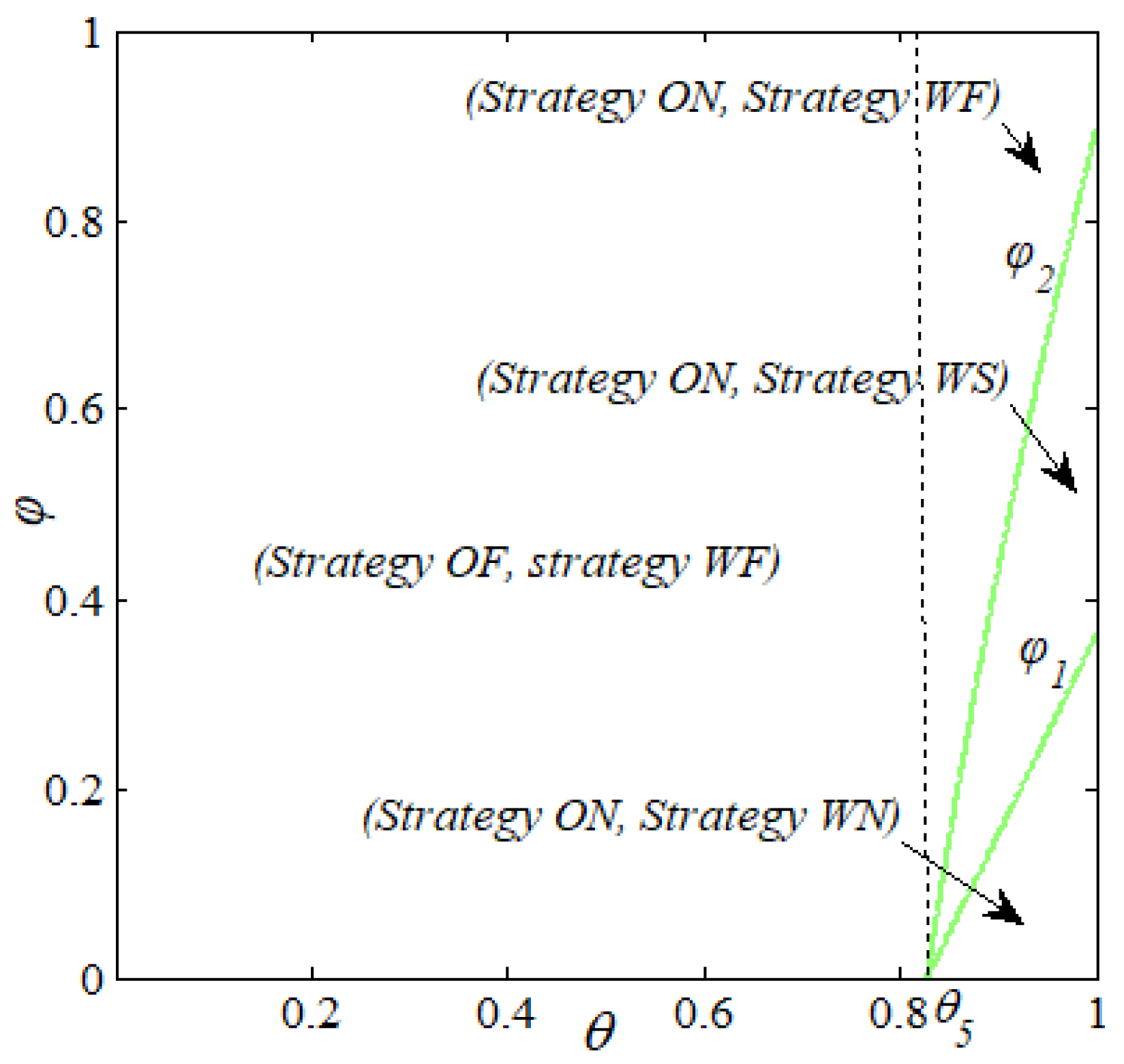
Proof of Proposition 6. Based on the equilibrium results in Lemmas 4–6, we obtain that , , , where , and . Based on the multiple-order differentiation with parameter to reduce the power exponent, we verify that , and increase in . Due to the fact that , and increases in , it suffices to find that if or and , if and , where is a unique solution of and is a unique solution of . Similarly, we find that if or and , if and , where is a unique solution of ; if or and , if and , where is a unique solution of . Note that when , and , that is, and , it suffices to find that . Based on the aforementioned results, we verify that when , ; when and , ; when and , ; when and , . □
Proof of Proposition 7. Based on the analytical results in Propositions 5 and 6, it is clear that when , and ; when , and if , and if , and if .
Moreover, we have employed a numerical experiment design to verify the robustness of the analytical results pertaining to the retailer’s encroachment decisions with/without the supplier learning effect and interaction mechanisms between private label encroachment cases (i.e., no encroachment, first-period encroachment, and second-period encroachment) and the supplier learning effect, as shown in Propositions 5–7. Below, we detail the design of this numerical experiment and validate the practical reproduction of our analytical results, which are summarized in
Table A1.
Table A1.
The numerical experiment of analytical results.
Table A1.
The numerical experiment of analytical results.
| Assignment of Market Parameters | Profit Comparison |
|---|
Without the supplier learning effect
(Proposition 5) | ; c | | ,
| |
| ; c | | ,
| |
With the supplier learning effect
(Proposition 6) | ; c | | ,
| |
| ,
|
| ,
|
| | ,
| |
| ,
| |
| ,
| |
Interaction mechanisms between private label encroachment and the supplier learning effect
(Proposition 7) | ; c | | |
| | |
| |
| |
Proof of Proposition 8. Based on the equilibrium results in Lemmas 1–3, we find that , , , , . A similar calculation leads to the analytical results for consumer surplus and social welfare among scenarios ON, OF and OS, as shown in Propositions 8(2). □
Proof of Proposition 9. Based on the equilibrium results of Lemmas 4–6, we find that , , , , , , , , where , , , , , , . Similarly, based on the multiple-order differentiation with parameter to reduce the power exponent, we verify that , , , , , and . As such, , , , , and . A similar algebraic calculation leads to the analytical results for consumer surplus and social welfare among scenarios WN, WF and WS, as shown in Propositions 9(2). □