Extragradient Algorithms for Solving Certain Nonlinear Problems with Application to Image Restorations

Abstract

In this paper, we introduced an inertial extragradient algorithm to approximate the common solution of split fixed point, split variational inclusion and split equilibrium problems involving nonexpansive mappings and pseudomonotone Lipschitz-type bifunctions in Hilbert spaces. Moreover, using some assumptions on the control parameters, we prove the strong convergence of the proposed algorithm and then apply our main result to solve the split minimization, split feasibility and split variational inequality problems. We also present some numerical examples to show the effectiveness and applicability of the proposed scheme. We include tables illustrating the number of iterations, the CPU time for convergence, comparisons among different algorithms, and the error analysis. We apply our proposed scheme to solve the image restoration problem as another application of the result presented herein.

1. Introduction

Throughout this paper, we denote N, $R^{+}$ and R as the set of all natural numbers, the set of positive real numbers and real numbers, respectively. The set given by $\mathcal{F}\left(T\right)=\{p^{\ast }\in \mathcal{C}:p^{\ast }=T{p}^{\ast }\}$ denotes the set of fixed points of T, where $T:\mathcal{C}\to \mathcal{C}$ is a mapping. A mapping T is called Lipschitz if for all $p,q\in \mathcal{C}$, there is a constant $c>0$ such that $\parallel Tp-Tq\parallel \le c\parallel p-q\parallel$ holds. If we restrict c in the interval $(0,1),$ then T is called a contraction, for $c=1$, T is nonexpansive.

The fixed points of nonexpansive mappings rely on the geometrical structure of fundamental space instead of topological properties such as compactness and weak compactness. Also, these mappings appear in differential inclusions involving dissipative or accretive mappings. Many nonlinear problems such as convex optimization, monotone inclusions, image restoration and variational inequality problems can be modeled as operator equations involving nonexpansive mappings; for details, see for example [1,2]. Furthermore, there is a strong connection between nonexpansive mappings (with respect to the hyperbolic metric) and the holomorphic mappings on the unit ball in the Hilbert space (see [3,4]). The classical examples of nonexpansive mappings are resolvent operators and metric projections.

Recall that a multivalued mapping $T:\mathcal{H}\to 2^{\mathcal{H}}$ is monotone if $\langle p-q,u-v\rangle \ge 0,$ where $p,q\in \mathcal{H}$, $u\in Tp$ and $v\in Tq$, and T is called maximal monotone if its graph is not properly contained in the graph of any other monotone mapping. Let $\eta >0$, define

$$J(\eta ;T)=J_{\eta }^T={(I+\eta T)}^{-1};$$

the operator $J_{\eta }^T$ is known as the resolvent of the operator T, and I is the identity mapping. If T maximal monotone then $J_{\eta }^T$ is single valued nonexpansive mapping and $J_{\eta }^T:R(I+\eta T)\to D\left(T\right).$

For any $p\in \mathcal{H}$, there is a unique element $P_{\mathcal{C}}p\in \mathcal{C}$ with

$$\parallel p-P_{\mathcal{C}}p\parallel =\inf \{\parallel p-q\parallel \mathrm{where}q\in \mathcal{C}\}.$$

where $P_{\mathcal{C}}:\mathcal{H}\to \mathcal{C}$ is known as metric projection.

An important characterization of the metric projection is as follows: for any $p\in \mathcal{H}$,

$$P_{\mathcal{C}}p=q\mathrm{iff}\langle p-q,q-r\rangle \ge 0,\forall r\in \mathcal{C}.$$

(1)

For more details about metric projections, we refer to [3,5].

1.1. Some Nonlinear Problems

In the sequel, $\mathcal{H},{\mathcal{H}}_1,{\mathcal{H}}_2$ denote the Hilbert spaces, $\mathcal{C}$ and $\mathcal{Q}$ are nonempty closed and convex subsets of ${\mathcal{H}}_1$ and ${\mathcal{H}}_2$, respectively, and $L:{\mathcal{H}}_1\to {\mathcal{H}}_2$ is a bounded linear operator with $L^{\ast }$ as its adjoint.

Let $T:\mathcal{C}\to \mathcal{C}$ be a mapping. Define the fixed point problem as

$$\mathrm{Find} p^{\ast }\in \mathcal{C} \mathrm{with} T{p}^{\ast }=p^{\ast }.$$

Solving the differential and integral equation problems is same as solving the fixed point problem of certain operators on functional spaces. These problems play a key role in modeling equilibrium states and analyzing stability across various fields such as economics, engineering, and image processing. Furthermore, it can be equivalently formulated as a variational inequality problem, an optimization problem, or a split feasibility problem, among others.

Moreover, the split fixed point problem is given by: find $p^{\ast }\in \mathcal{C}$ such that

$$T{p}^{\ast }=p^{\ast } \mathrm{with}L{p}^{\ast }\in \mathcal{Q} \mathrm{and} S\left(L{p}^{\ast }\right)=L{p}^{\ast },$$

where, T and S are self mappings on $\mathcal{C}$ and $\mathcal{Q}$, respectively, and $L:\mathcal{C}\to \mathcal{Q}$ is a nonlinear operator.

Define the equilibrium problem (EP): Find a point $p^{\ast }\in \mathcal{C}$ such that

$$F(p^{\ast },q)\ge 0,\forall q\in \mathcal{C},$$

(2)

where, $F:\mathcal{C}\times \mathcal{C}\to R$ is a bifunction.

Equilibrium problems provide a unified approach for modeling and solving complex problems in economics, game theory, and engineering.

The split equilibrium problem (SEP) is defined as follows: Find a point $p^{\ast }\in \mathcal{C}$ such that

$$F_1(p^{\ast },q)\ge 0,\forall q\in \mathcal{C},\mathrm{such}\mathrm{that}L{p}^{\ast }\in \mathcal{Q}\mathrm{and}{F}_2(L{p}^{\ast },r)\ge 0,\forall r\in \mathcal{Q}.$$

(3)

where, $F_1$ and $F_2$ are real-valued bifunctions on $\mathcal{C}\times \mathcal{C}$ and $\mathcal{Q}\times \mathcal{Q}$, respectively.

The variational inequality problem (VIP) is defined as follows: Find a point $p^{\ast }\in \mathcal{C}$ such that

$$\langle T{p}^{\ast },q-p^{\ast }\rangle \ge 0,\forall q\in \mathcal{C},$$

(4)

where the operator $T:\mathcal{C}\to \mathcal{H}$ is nonlinear.

Remark 1.

If we set $F(p,q)=\langle Tp,q-p\rangle \forall q,p\in \mathcal{C}$, then the VIP (4) is equivalent to EP (3).

The variational inequality has focused the considerable attention of many authors because of its ability to model a wide range of problems of a practical nature, including optimal control, image processing, and signal processing, for further details, see [6,7,8,9]. Furthermore, the split inverse problem (SIP) is given as follows:

Find a point

$$p^{\ast }\in {\mathcal{H}}_1 \mathrm{that} \mathrm{can} \mathrm{solve} {\mathcal{I}}_1, \mathrm{with} Lp\ast \in {\mathcal{H}}_2 \mathrm{that} \mathrm{can} \mathrm{can} \mathrm{solve}{\mathcal{I}}_2,$$

where ${\mathcal{I}}_1$ and ${\mathcal{I}}_2$ are the inverse problems in ${\mathcal{H}}_1$ and ${\mathcal{H}}_2$, respectively.

Now, we define the split variational inclusion problem (SVIP) as follows:

Let $M_1:{\mathcal{H}}_1\to 2^{{\mathcal{H}}_1}$ and $M_2:{\mathcal{H}}_2\to 2^{{\mathcal{H}}_2}$ be two mappings which are maximal monotone. The SVIP is given by

$$p^{\ast }\in {\mathcal{H}}_1 \mathrm{with} 0\in M_1\left(p^{\ast }\right),$$

and

$$L{p}^{\ast }\in {\mathcal{H}}_2, \mathrm{such} \mathrm{that} 0\in M_2\left(L{p}^{\ast }\right).$$

Furthermore, SVIPs have many practical applications (see [10,11]).

Remark 2.

From [12,13], the following observations hold:

$\left(i\right)$

The map M is a maximal monotone if $J_{\eta }^M$ is a single-valued map.

$\left(ii\right)$

$J_{\eta }^M{p}^{\ast }=p^{\ast }$ if $p^{\ast }\in M^{-1}\left(0\right).$

$\left(iii\right)$

The SVIP is given as follows:

Find $p^{\ast }\in {\mathcal{H}}_1$ with

$$J_{{\eta }_1}^{M_1}{p}^{\ast }=p^{\ast }\mathit{such}\mathit{that}L{p}^{\ast }\in {\mathcal{H}}_2\mathit{and}L{p}^{\ast }=J_{\eta 2}^{M_2}L{p}^{\ast }.$$

(5)

1.2. Review of Some Iterative Algorithms

Since the approximation of fixed points for the class of nonexpansive mappings has been observed extensively with the help of iterative algorithms (see [14,15]). Many algorithms have been proposed and applied in this direction, for instance, Abbas et al. [16] proposed the AA-algorithm, which is described as follows in Algorithm 1.

Algorithm 1 AA-algorithm from Abbas et al. [16]

Initialization: Take $\left\{{\alpha }_n\right\}$, $\left\{{\beta }_n\right\}$ and $\left\{{\gamma }_n\right\}$ as control parameters in $(0,1)$. Choose any $p_1\in \mathcal{C}$, define $p_{n+1}$ as: $$\begin{array}{c}{s}_n=(1-{\gamma }_n)p_n+{\gamma }_{n}T{p}_n,\hfill \\ r_n=T((1-{\beta }_n)s_n+{\beta }_{n}T{s}_n),\hfill \\ q_n=T((1-{\alpha }_n)T{s}_n+{\alpha }_{n}T{r}_n),\hfill \\ p_{n+1}=T{q}_n.\hfill \end{array}$$

The authors in [16] claimed that the AA-algorithm converges faster than other comparable existing algorithms. After that, many researchers used the AA-algorithm to obtain the solutions of nonlinear problems, see [17,18,19,20].

Further, Byrne et al. [21] introduced the algorithm to find the solution of the SVIP using maximal monotone operators $M_1$ and $M_2$ and presented in Algorithm 2.

Algorithm 2 Algorithm proposed in Byrne et al. [21]

Initialization: Let $\left\{{\alpha }_n\right\}\subset (0,1)$, $\eta >0$, and $\omega \in \left(0,{\displaystyle \frac{2}{L}}\right)$, where $L=\parallel A^{\ast }A\parallel$. Select $p_1\in {\mathcal{H}}_1$. Define the sequence $\left\{p_n\right\}$ by $$p_{n+1}={\alpha }_n{p}_n+(1-{\alpha }_n)J_{\eta }^{M_1}\left(p_n+\omega A^{\ast }(J_{\eta }^{M_2}-I)A{p}_n\right),$$ where ${\lim }_{n\to \infty }{\alpha }_n=0$ and ${\sum }_{n=1}^{\infty }{\alpha }_n=\infty$.

To find the common solution of FPP and SVIP, the following algorithm was proposed in [22] and given in Algorithm 3.

Algorithm 3 Algorithm proposed in Wangkeeree et al. [22]

Initialization: Assume $\left\{{\alpha }_n\right\}\in (0,1)$, $\eta >0$, $\omega \in (0,{\displaystyle \frac{2}{L}})$, here L is spectral radius of $A^{\ast }A$. Take any $p_1\in {\mathcal{H}}_1$, find $p_{n+1}$ as: $$q_n=J_{\eta }^{M_1}(p_n+\omega A^{\ast }(J_{\eta }^{M_2}-I)A{p}_n)$$ $$p_{n+1}={\alpha }_n\eta f\left(p_n\right)+(1-{\alpha }_{n}B)S{q}_n,$$ The f is contraction and S is a nonexpansive self mapping on ${\mathcal{H}}_1$, $B:{\mathcal{H}}_1\to {\mathcal{H}}_1$ is linear and $M_1:{\mathcal{H}}_1\to 2^{{\mathcal{H}}_1}$ and $M_2:{\mathcal{H}}_2\to 2^{{\mathcal{H}}_2}$ are the maximal monotone.

The authors in [22] have shown the strong convergence of the sequence to the common solution of FPP and SVIP. Furthermore, to obtain the common solution, SVIP remains the focus of many authors, for some recent work in this direction, we refer to [23,24].

The convergence rate of an iterative algorithm relies on its construction and the selection of step sizes. By choosing an appropriate step size, one can approximate the solution in a fewer number of steps. Since, in the Algorithms 2 and 3, the step size depend upon the operator norm, and it is indeed difficult to find the exact operator norm or it is too expensive to compute. To overcome this problem, Tang [12] modified Algorithm 2 with a step size that is independent of this requirement and obtained the solution of SVIP. An algorithm thus developed is presented in Algorithm 4.

Algorithm 4 Algorithm proposed in Tang [12]

Initialization: Let $\left\{{\lambda }_n\right\}$ be a sequence in ${\lambda }_n\subset (0,4)$ with $\inf {\lambda }_n(4-{\lambda }_n)>0$. Find $${\omega }_n={\displaystyle \frac{{\lambda }_{n}g\left(p_n\right)}{\parallel G{p}_n{\parallel }^2+{\parallel H{p}_n\parallel }^2}},$$ compute $$p_{n+1}={\alpha }_n{p}_n+(1-{\alpha }_n)J_{\eta }^{M_1}(p_n-{\omega }_n{A}^{\ast }(I-J_{\eta }^{M_2})A{p}_n),$$ where $g\left(p\right)={\displaystyle \frac{1}{2}}\parallel (I-J_{{\eta }_1}^{M_2})Ap{\parallel }^2$, $G\left(p\right)=A^{\ast }(I-J_{{\eta }_1}^{M_2})Ap$, $H\left(p\right)=(I-J_{{\eta }_1}^{{\beta }_2})p$.

Many authors have proposed different algorithms by incorporating the inertial technique for accelerating the convergence rate of an algorithm, for instance, see [25,26,27,28].

Continuing in this direction, Narin et al. [29] proposed the following extragradient algorithm, which is given in Algorithm 5 as follows:

Algorithm 5 Extragradient algorithm proposed in Narin et al. [29]

Initialization: Under certain assumptions on the controlled parameters, choose any $p_1\in {\mathcal{H}}_1$; Find $p_{n+1}$ as follows: $$\begin{array}{c}{v}_n=arg\min \left\{{\theta }_n\psi (P_{\mathcal{Q}}\left(L{p}_n\right),u)+{\displaystyle \frac{1}{2}}{\parallel u-P_{\mathcal{Q}}\left(L{p}_n\right)\parallel }^2:u\in \mathcal{Q}\right\},\hfill \\ u_n=arg\min \left\{{\theta }_n\psi (v_n,u)+{\displaystyle \frac{1}{2}}{\parallel u-P_{\mathcal{Q}}\left(L{p}_n\right)\parallel }^2:u\in \mathcal{Q}\right\},\hfill \\ q_n=P_{\mathcal{C}}\left(p_n+{\zeta }_n{L}^{\ast }(S{u}_n-L{p}_n)\right),\hfill \\ s_n=arg\min \left\{{\sigma }_n\varphi (q_n,q)+{\displaystyle \frac{1}{2}}{\parallel q-q_n\parallel }^2:q\in \mathcal{C}\right\},\hfill \\ r_n=arg\min \left\{{\sigma }_n\varphi (s_n,q)+{\displaystyle \frac{1}{2}}{\parallel q-q_n\parallel }^2:q\in \mathcal{C}\right\},\hfill \\ p_{n+1}={\alpha }_{n}f\left(p_n\right)+(1-{\alpha }_n)\left({\beta }_n{p}_n+(1-{\beta }_n)T{r}_n\right).\hfill \end{array}$$

The authors showed the strong convergence of Algorithm 5, which involves pseudomonotone bifunctions and Lipschitzian nonexpansive mappings. However, to obtain the solution of the same problem, Ezeora et al. [30] modified Algorithm 5 by adding the inertial step size to speed up the algorithm, which is given in Algorithm 6.

Algorithm 6 Extragradient algorithm proposed in Ezeora et al. [30]

Initialization: Under appropriate assumptions on the controlled parameters, choose any $p_1\in {\mathcal{H}}_1$; Find $p_{n+1}$ as follows: $$\begin{array}{c}{w}_n=x_n+{\pi }_n(p_n-p_{n-1}),\hfill \\ v_n=arg\min \left\{{\theta }_n\psi (P_{\mathcal{Q}}\left(L{w}_n\right),u)+{\displaystyle \frac{1}{2}}{\parallel u-P_{\mathcal{Q}}\left(L{w}_n\right)\parallel }^2:u\in \mathcal{Q}\right\},\hfill \\ u_n=arg\min \left\{{\theta }_n\psi (v_n,u)+{\displaystyle \frac{1}{2}}{\parallel u-P_{\mathcal{Q}}\left(L{w}_n\right)\parallel }^2:u\in \mathcal{Q}\right\},\hfill \\ q_n=P_{\mathcal{C}}\left(p_n+{\zeta }_n{L}^{\ast }(S{u}_n-L{w}_n)\right),\hfill \\ s_n=arg\min \left\{{\sigma }_n\varphi (q_n,q)+{\displaystyle \frac{1}{2}}{\parallel q-q_n\parallel }^2:q\in \mathcal{C}\right\},\hfill \\ r_n=arg\min \left\{{\sigma }_n\varphi (s_n,q)+{\displaystyle \frac{1}{2}}{\parallel q-q_n\parallel }^2:q\in \mathcal{C}\right\},\hfill \\ p_{n+1}={\alpha }_{n}f\left(w_n\right)+(1-{\alpha }_n)\left({\beta }_n{p}_n+(1-{\beta }_n)T{r}_n\right).\hfill \end{array}$$

Although several inertial and extragradient-type algorithms with strong convergence have been proposed in recent years, most existing methods focus on a single problem class, such as variational inequalities or split variational inclusions; see, for example, [6,7,31,32]. Moreover, some recent approaches employ multiple inertial terms or require stronger assumptions on operators. In contrast, the proposed algorithm integrates viscosity regularization, a single inertial extrapolation, and an extragradient step into a unified framework for computing a common solution of split fixed point, split variational inclusion, and split equilibrium problems. This unified treatment allows us to establish strong convergence under standard assumptions while covering a broader class of coupled problems.

Remark 3.

Various algorithms were proposed in the existing literature to approximate solutions to the aforementioned nonlinear problems; however, they have certain limitations. For instance, the algorithms proposed in [29,33,34] do not involve the inertial term, which plays a significant role to speed up the rate of convergence of an algorithm. Moreover, these algorithms require the prior knowledge of the norm of a bounded linear operator involved therein. Similarly, the algorithms defined in [35,36] involve the monotone bifunctions and have the limited applications. The algorithms used in [29,30] require a large number of iterations and hence consume much CPU time for their convergence in the case of very high dimensions; see Table 1, Table 2 and Table 3. Moreover, these algorithms typically approximate a common solution for only two nonlinear problems, which limits their range of applications.

Remark 4.

Many problems arising in optimization, equilibrium theory and inverse problems can be modeled as fixed-point problems, variational inclusions, or equilibrium problems, often coupled through linear operators. In practical applications, such as image restoration and signal processing, these problems usually appear together rather than in isolation, and a solution is required to satisfy all models simultaneously. The study of a common solution framework allows these related problems to be handled in a unified way, which protects against solving each problem separately and sequentially. This unified approach not only reduces computational cost but also leads to algorithms with stronger theoretical guarantees and better numerical stability. Moreover, the common solution formulation naturally connects with recent developments in split problems and operator splitting methods, making it well suited for modern applications involving coupled constraints and multi-model systems.

If we think, is it possible to construct an algorithm that has a good convergence rate and is able to find the unified solution of more general nonlinear problems without the operator norm and require fewer iterative steps with CPU time? Motivated by the above directions and the AA-algorithm, the aim of this paper is to propose an efficient algorithm with the inertial term, independent of the norm of the operator and the self-adaptive step size, as opposed to the methods described above. It enables us to solve certain nonlinear problems at a time in a fewer number of steps with less CPU time than the above-mentioned algorithms. Moreover, it involves the pseudomonotone bifunctions, a more general class than the class of monotone mappings, and hence extends the scope of applications. We obtained a strong convergence result to approximate the common solution of SVIP, SEP and SFP using appropriate control parameters. These problems have applications in fields such as signal and image processing, network resources, and others (see, for details, [37,38]). Finally, we apply our algorithm to solve the image restoration problem and compare it with the comparable method proposed in [39] with respect to peak signal-to-noise ratio and the CPU time, which shows the potential of our iterative algorithm presented herein.

2. Preliminaries

Definition 1.

A mapping T from $\mathcal{C}$ onto $\mathcal{H}$ is said to be firmly nonexpansive if, for any $p,q\in \mathcal{C}$, the following holds:

$$\langle Tp-Tq,p-q\rangle \ge {\parallel Tp-Tq\parallel }^2.$$

Note that $P_{\mathcal{C}}$ is an example of firmly nonexpansive mapping and hence nonexpansive. For further details on firmly nonexpansive mappings, we refer the reader to [3].

Definition 2.

If ϕ is a bifunction such that $\varphi :\mathcal{C}\times \mathcal{C}\to R$, we say ϕ is:

$\left(i\right)$

Monotone on $\mathcal{C}$ if

$$\varphi (p,q)+\varphi (q,p)\le 0,\forall p,q\in \mathcal{C}.$$

$\left(ii\right)$

Pseudomonotone on $\mathcal{C}$ if $\varphi (p,q)\ge 0$ implies that $\varphi (q,p)\le 0,\forall p,q\in \mathcal{C}$.

$\left(iii\right)$

Lipschitzian-type if we have ${\mu }_1,{\mu }_2>0$ (called Lipschitzian constants) such that:

$$\varphi (p,r)-{\mu }_1{\parallel p-q\parallel }^2-{\mu }_2{\parallel q-r\parallel }^2\le \varphi (p,q)+\varphi (q,r),\forall p,q,r\in \mathcal{C}.$$

Definition 3.

The subdifferential of a mapping ϕ denoted by $\partial \varphi$ and defined as follows:

$$\partial \varphi \left(p\right)=\{q\in \mathcal{H}:\varphi p-\varphi r\le \langle q,p-r\rangle \forall r\in \mathcal{H}\},\mathit{for}\mathit{each}p\in \mathcal{H}.$$

Definition 4.

The normal cone $N_{\mathcal{C}}{p}_0$ at $p_0\in \mathcal{C}$ is defined by

$$N_{\mathcal{C}}{p}_0=\{p\in \mathcal{H}:\langle p,q-p_0\rangle \le 0,\forall q\in \mathcal{C}\}.$$

Lemma 1

([40]). If $p,q\in \mathcal{H}$ and $\xi \in R,$ then we have the followings:

(i) 

${\parallel p+q\parallel }^2\le {\parallel p\parallel }^2+2\langle p+q,q\rangle$,

(ii) 

${\parallel p+q\parallel }^2={\parallel p\parallel }^2+2\langle p,q\rangle +{\parallel q\parallel }^2$,

(iii) 

${\parallel p-q\parallel }^2={\parallel p\parallel }^2-2\langle p,q\rangle +{\parallel q\parallel }^2$,

(iv) 

${\parallel \xi p+(1-\xi )q\parallel }^2={\xi \parallel p\parallel }^2{-\xi (1-\xi )\parallel p-q\parallel }^2+(1-\xi ){\parallel q\parallel }^2$.

Lemma 2

([41]). Assume that $\left\{{\overline{x}}_n\right\},\left\{{\overline{z}}_n\right\}\in R^{+}$ with ${\sum }_{n=0}^{\infty }{\overline{z}}_n<\infty$, $\left\{{\overline{y}}_n\right\}\subset R$, $\left\{{\xi }_n\right\}\subset (0,1)$ and

$${\overline{x}}_{n+1}\le (1-{\xi }_n){\overline{x}}_n+{\overline{y}}_n+{\overline{z}}_n,\forall n\ge 0.$$

(i) 

If ${\overline{y}}_n\le k{\xi }_n$, where $k\ge 0,$ then $\left\{{\overline{x}}_n\right\}$ is bound.

(ii) 

If ${\sum }_{n=0}^{\infty }{\xi }_n=\infty$ with $\underset{n\to \infty }{\lim \sup }{\displaystyle \frac{{\overline{y}}_n}{{\xi }_n}}\le 0,$ then $\underset{n\to \infty }{\lim }{\overline{x}}_n\to 0$.

Lemma 3

([42]). If T is a self-nonexpansive mapping on $\mathcal{H}$ with $\mathcal{F}\left(T\right)\ne \varnothing$. Then $I-T$ is demi-closed at zero, which means, for each $\left\{p_n\right\}$ in $\mathcal{H}$, with

$$p_n\rightharpoonup p^{\ast }\mathit{and}\parallel p_n-T{p}_n\parallel \to 0,$$

we have $p^{\ast }\in \mathcal{F}\left(T\right)$.

Lemma 4

([43]). Assume that $\left\{{\overline{x}}_n\right\}\subset R^{+}$, $\left\{{\overline{y}}_n\right\}\subset R$, $\left\{{\sigma }_n\right\}\subset (0,1)$ and ${\sum }_{n=0}^{\infty }{\sigma }_n=\infty$ and $\left\{{\overline{y}}_n\right\}\subset R$ with 

$${\overline{x}}_{n+1}\le (1-{\sigma }_n){\overline{x}}_n+{\sigma }_n{\overline{y}}_n.$$

If $\underset{n\to \infty }{\lim \sup } {\overline{y}}_{n_i}\le 0$, and for each subsequence $\left\{{\overline{x}}_{n_i}\right\}$ of $\left\{{\overline{x}}_n\right\}$ with $\underset{n\to \infty }{\lim \inf }({\overline{x}}_{n_{i+1}}-{\overline{x}}_{n_i})\ge 0,$ then $\underset{n\to \infty }{\lim }{\overline{x}}_n=0.$

Lemma 5

([44]). If $\left\{p_n\right\}\in \mathbb{R}$ and there exists a subsequence such that $p_{n_i}<p_{n_i+1}$. Then, there is the sequence $\left\{m_k\right\}$, which is nondecreasing with $m_k\to \infty$ and

$$p_{m_k}\le p_{m_{k+1}}\mathit{and}{p}_k\le p_{m_{k+1}}.$$

where $m_k=\max \{j\le k:p_j<p_{j+1}\}$.

3. Convergence Results

Assumption 1.

If $\mathcal{C}\subset \mathcal{H}$ and $\varphi :\mathcal{C}\times \mathcal{C}\to R$ are bifunctions, the following apply:

$\left(A_1\right)$

 ϕ is a pseudomonotone mapping on $\mathcal{C}$ and $\varphi (p,p)=0$, for all $p\in \mathcal{C}$.

$\left(A_2\right)$

 ϕ is a weakly continuous mapping on $\mathcal{C}\times \mathcal{C}$.

$\left(A_3\right)$

 $\varphi (.,p)$ is convex and subdifferentiable on $\mathcal{C}$ for each fixed p.

$\left(A_4\right)$

 ϕ is Lipschitz-type continuous on $\mathcal{C}$ with Lipschitzian constants ${\mu }_1,{\mu }_2>0,$ which is

$$\varphi (p,r)-{\mu }_n{\parallel p-q\parallel }^2-{\mu }_2{\parallel q-r\parallel }^2\le \varphi (p,q)+\varphi (q,r),\forall p,q,r\in \mathcal{C}.$$

Proposed Algorithm

Let us set the following notations:

Suppose that $M_1:{\mathcal{H}}_1\to 2^{{\mathcal{H}}_1}$ and $M_2:{\mathcal{H}}_2\to 2^{{\mathcal{H}}_2}$ are maximal monotone mappings, $\varphi :\mathcal{C}\times \mathcal{C}\to \mathbb{R}$ and $\psi :\mathcal{Q}\times \mathcal{Q}\to \mathbb{R}$ satisfy the conditions $(i–ii)$ in Assumption 1, and $L:{\mathcal{H}}_1\to {\mathcal{H}}_2$ is bounded linear operator with $L^{\ast }$ as its adjoint. Let $T:\mathcal{C}\to \mathcal{C}$ and $S:\mathcal{Q}\to \mathcal{Q}$ be nonexpansive mappings and $f:{\mathcal{H}}_1\to {\mathcal{H}}_1$ satisfies the contractive condition with contraction constant c.

Define the following mappings as follows:

$$\begin{array}{cc}\hfill a\left(p\right)=& {\displaystyle \frac{1}{2}}\parallel (I-J_{{\eta }_2}^{M_2})Lp{\parallel }^2,b\left(p\right)={\displaystyle \frac{1}{2}}\parallel (I-J_{{\eta }_1}^{M_1})p{\parallel }^2,\hfill \\ \hfill A\left(p\right)=& L^{\ast }(I-J_{{\eta }_2}^{M_2})Lp,B\left(p\right)=(I-J_{{\eta }_1}^{M_1})p.\hfill \end{array}$$

where a and b are convex, differentiable and weakly lower semi-continuous [45]. Also, A and B are Lipschitzian [12]. Now we present our proposed technique and given in Algorithm 7.

Choose ${\delta }_n$ as follows: ${\delta }_n\in \left(ϵ,{\displaystyle \frac{\parallel L{w}_n-S{u}_n{\parallel }^2}{\parallel L^{\ast }(L{w}_n-S{u}_n){\parallel }^2}}-ϵ\right)$ if $L{w}_n-S{u}_n\ne 0$, otherwise take ${\delta }_n$ equal to $\delta$, which is a nonnegative real number. The other control parameters in the above algorithm satisfy the following conditions:

(i)

$\left\{{\alpha }_n\right\}\in \left(0,{\displaystyle \frac{1}{2(1-c)}}\right),$ with ${\lim }_{n\to \infty }{\alpha }_n=0$ and ${\sum }_{n=0}^{\infty }{\alpha }_n=\infty$.

(ii)

$\left\{{\beta }_n\right\},\left\{{\gamma }_n\right\}\in (0,1)$.

(iii)

$\kappa >0$ is fixed and $\left\{{\theta }_n\right\}\in {\mathbb{R}}^{+}$ with ${\lim }_{n\to \infty }{\displaystyle \frac{{\theta }_n}{{\alpha }_n}}=0.$

(iv)

$0<{\sigma }_1\le {\sigma }_n\le {\sigma }_2<\min \left\{{\displaystyle \frac{1}{{\mu }_1}},{\displaystyle \frac{1}{{\mu }_2}}\right\}$.

(v)

$0<{\theta }_1\le {\theta }_n\le {\theta }_2<\min \left\{{\displaystyle \frac{1}{o_1}},{\displaystyle \frac{1}{o_2}}\right\}$.

(vi)

$0<{\lambda }_n<4$ and ${\eta }_i>0$ for $i\in \{1,2\}.$

Remark 5.

By using the above conditions, we have

$$\underset{n\to \infty }{\lim }{\displaystyle \frac{{\kappa }_n}{{\alpha }_n}}\parallel p_n-p_{n-1}\parallel =0.$$

Define the following problem:

Find $p^{\ast }\in \mathcal{F}\left(T\right)\cap \mathcal{EP}\left(\varphi \right)\cap \mathcal{VIP}\left(M_1\right)$ such that $L{p}^{\ast }\in \mathcal{F}\left(S\right)\cap \mathcal{EP}\left(\psi \right)\cap \mathcal{VIP}\left(M_2\right)$. Suppose that $\mathsf{\Omega }$ is the solution set of the above problem and $P_{\mathsf{\Omega }}:{\mathcal{H}}_1\to \mathsf{\Omega }$ is a mapping.

Lemma 6

([46]). Suppose that ϕ satisfies Assumption 1 such that $\mathcal{EP}\left(\varphi \right)\ne \varnothing .$ Set

$$0<j_0<\min \left\{{\displaystyle \frac{1}{2{\mu }_1}},{\displaystyle \frac{1}{2{\mu }_2}}\right\}.$$

If $p_0\in \mathcal{C}$ and define $q_0$ and $r_0$ as follows:

$$q_0=arg\min \left\{j_0\varphi (p_0,q)+{\displaystyle \frac{1}{2}}{\parallel q-p_0\parallel }^2:q\in \mathcal{C}\right\}.$$

and

$$r_0=arg\min \left\{j_0\varphi (q_0,q)+{\displaystyle \frac{1}{2}}{\parallel q-p_0\parallel }^2:q\in \mathcal{C}\right\}.$$

Then, for all $p^{\ast }\in \mathcal{EP}\left(\varphi \right),$ we have the following:

(i) 

$j_0[\varphi (p_0,q)-\varphi (p_0,q_0)]\ge \langle q_0-p_0,q_0-p\rangle ,$ for all $q\in \mathcal{C}.$

(ii) 

$\parallel r_0-p^{\ast }{\parallel }^2 \le \parallel p_0-p^{\ast }{\parallel }^2-(1-2j_0{\mu }_1)\parallel p_0-q_0{\parallel }^2-(1-2j_0{\mu }_2){\parallel q_0-r_0\parallel }^2$.

Algorithm 7 Proposed inertial extragradient algorithm

Initialization: Let $p_0,p_1\in {\mathcal{H}}_1$, $\kappa \in [0,1)$, and $ϵ>0$ be sufficiently small. Step 1. Let ${\sum }_{n=1}^{\infty }{\theta }_n<\infty$ and choose ${\kappa }_n$ such that ${\displaystyle {\kappa }_n\in [0,{\widehat{\kappa }}_n],{\widehat{\kappa }}_n=\left\{\begin{array}{cc}\min \left\{\kappa ,\frac{{\theta }_n}{\parallel p_n-p_{n-1}\parallel }\right\},\hfill & p_n\ne p_{n-1}\hfill \\ \kappa ,\hfill & \mathrm{otherwise}.\hfill \end{array}\right.}$ Step 2. Compute $${\displaystyle w_n=p_n+{\kappa }_n(p_n-p_{n-1}).}$$ Step 3. Calculate $${\displaystyle v_n=arg\min \left\{{\theta }_n\psi \left(P_{\mathcal{Q}}\left(L{w}_n\right),v\right)+\frac{1}{2}{\parallel v-P_{\mathcal{Q}}\left(L{w}_n\right)\parallel }^2:v\in \mathcal{Q}\right\}.}$$ Step 4. Find $${\displaystyle u_n=arg\min \left\{{\theta }_n\psi (v_n,v)+\frac{1}{2}{\parallel v-P_{\mathcal{Q}}\left(L{w}_n\right)\parallel }^2:v\in \mathcal{Q}\right\}.}$$ Step 5. Find $${\displaystyle q_n=P_{\mathcal{C}}\left(w_n+{\delta }_n{L}^{\ast }(S{u}_n-L{w}_n)\right).}$$ Step 6. Compute $${\displaystyle s_n=arg\min \left\{{\sigma }_n\varphi (q_n,q)+\frac{1}{2}{\parallel q-q_n\parallel }^2:q\in \mathcal{C}\right\}.}$$ Step 7. Calculate $${\displaystyle r_n=arg\min \left\{{\sigma }_n\varphi (s_n,q)+\frac{1}{2}{\parallel q-q_n\parallel }^2:q\in \mathcal{C}\right\}.}$$ Step 8. Set $${\displaystyle x_n={\gamma }_n{w}_n+(1-{\gamma }_n)r_n.}$$ Step 9. Find $${\displaystyle t_n=J_{{\eta }_1}^{M_1}\left(I-{\zeta }_n{L}^{\ast }(I-J_{{\eta }_2}^{M_2})L\right)x_n,}$$ where $${\displaystyle {\zeta }_n=\left\{\begin{array}{cc}{\displaystyle \frac{{\lambda }_{n}a\left(x_n\right)}{\parallel A\left(x_n\right){\parallel }^2+{\parallel B\left(x_n\right)\parallel }^2}},\hfill & \parallel A\left(x_n\right){\parallel }^2+{\parallel B\left(x_n\right)\parallel }^2\ne 0,\hfill \\ 0,\hfill & \mathrm{otherwise}.\hfill \end{array}\right.}$$ Step 10. Compute $${\displaystyle y_n=T\left((1-{\beta }_n)x_n+{\beta }_{n}T{t}_n\right).}$$ Step 11. Update $${\displaystyle p_{n+1}={\alpha }_{n}f\left(w_n\right)+(1-{\alpha }_n)T{y}_n.}$$

Theorem 1.

Suppose that $\varphi ,\psi ,L,S,T,M_1,M_2$ and f are as above. If $\left\{p_n\right\}$ is given by Algorithm 7 and fulfills $\left(i\right)–\left(vi\right)$, then $\left\{p_n\right\}$ converges strongly to the fixed point of mapping $P_{\mathsf{\Omega }}of$.

Lemma 7.

The sequence $\left\{p_n\right\}$, defined in Algorithm 7 is bounded.

Proof. 

   Since $P_{\mathsf{\Omega }}of$ is a contraction based on the Banach contraction principle, there exists $p^{\ast }\in {\mathcal{H}}_1$ such that $P_{\mathsf{\Omega }}of\left(p^{\ast }\right)=p^{\ast }$ and $p^{\ast }\in \mathsf{\Omega }$. This gives us $T\left(p^{\ast }\right)=p^{\ast },S\left(L{p}^{\ast }\right)=L{p}^{\ast },J_{{\eta }_1}^{M_1}{p}^{\ast }=p^{\ast },J_{{\eta }_2}^{M_2}\left(L{p}^{\ast }\right)=L{p}^{\ast }.$ From Algorithm 7, we have

$$\begin{array}{cc}\hfill \parallel w_n-p^{\ast }\parallel & =\parallel p_n+{\kappa }_n(p_n-p_{n-1})-p^{\ast }\parallel \hfill \\ \hfill & \le \parallel p_n-p^{\ast }\parallel +{\kappa }_n\parallel p_n-p_{n-1}\parallel \hfill \\ \hfill & =\parallel p_n-p^{\ast }\parallel +{\alpha }_n{\displaystyle \frac{{\kappa }_n}{{\alpha }_n}}\parallel p_n-p_{n-1}\parallel .\hfill \end{array}$$

(6)

By Remark 5, we have ${\lim }_{n\to \infty }{\displaystyle \frac{{\kappa }_n}{{\alpha }_n}}\parallel p_n-p_{n-1}\parallel =0$, which implies that there exists a constant $C_1>0$ such that ${\displaystyle \frac{{\kappa }_n}{{\alpha }_n}}\parallel p_n-p_{n-1}\parallel \le C_1$, for all $n\ge 1$. Hence, by (6), we have

$$\parallel w_n-p^{\ast }\parallel \le \parallel p_n-p^{\ast }\parallel +{\alpha }_n{C}_1.$$

(7)

Using Lemma 1 and $P_{\mathcal{Q}}$ being firmly nonexpansive, we have

$$\begin{array}{cc}\hfill \parallel P_{\mathcal{Q}}\left(L{w}_n\right)-L{p}^{\ast }{\parallel }^2& =\parallel P_{\mathcal{Q}}\left(L{w}_n\right)-P_{\mathcal{Q}}\left(L{p}^{\ast }\right){\parallel }^2\hfill \\ \hfill & \le \langle P_{\mathcal{Q}}\left(L{w}_n\right)-P_{\mathcal{Q}}\left(L{p}^{\ast }\right),L{w}_n-L{p}^{\ast }\rangle \hfill \\ \hfill & =\langle P_{\mathcal{Q}}\left(L{w}_n\right)-L{p}^{\ast },L{w}_n-L{p}^{\ast }\rangle \hfill \\ \hfill & ={\displaystyle \frac{1}{2}}\left[\parallel P_{\mathcal{Q}}\left(L{w}_n\right)-L{p}^{\ast }{\parallel }^2+{\parallel L{w}_n-L{p}^{\ast }\parallel }^2\right.\hfill \\ \hfill & \left.-\parallel P_{\mathcal{Q}}\left(L{w}_n\right)-L{w}_n{\parallel }^2\right]\hfill \\ \hfill & =\parallel L{w}_n-L{p}^{\ast }{\parallel }^2-{\parallel P_{\mathcal{Q}}\left(L{w}_n\right)-L{w}_n\parallel }^2.\hfill \end{array}$$

(8)

Since S is nonexpansive, based on $L{p}^{\ast }\in \mathcal{F}\left(S\right)$ from Lemma 6, we get that

$$\begin{array}{cc}\hfill \parallel S{u}_n-L{p}^{\ast }{\parallel }^2& =\parallel S{u}_n-S\left(L{p}^{\ast }\right){\parallel }^2\hfill \\ \hfill & \le \parallel u_n-L{p}^{\ast }{\parallel }^2\hfill \\ \hfill & \le \parallel P_{\mathcal{Q}}\left(L{w}_n\right)-L{p}^{\ast }{\parallel }^2-(1-2{\theta }_n{o}_1){\parallel P_{\mathcal{Q}}\left(L{w}_n\right)-v_n\parallel }^2\hfill \\ \hfill & -(1-2{\theta }_n{o}_2){\parallel v_n-u_n\parallel }^2,\forall n\in \mathbb{N}.\hfill \end{array}$$

(9)

By using the assumptions (8) and (9), we have

$$\parallel S{u}_n-L{p}^{\ast }{\parallel }^2 \le \parallel L{w}_n-L{p}^{\ast }{\parallel }^2-{\parallel P_{\mathcal{Q}}\left(L{w}_n\right)-L{w}_n\parallel }^2.$$

(10)

From Lemma 1 and (10), we have

$$\begin{array}{cc}\hfill \langle L(w_n-p^{\ast }),S{u}_n-L{w}_n\rangle & =\langle S{u}_n-L{p}^{\ast },S{u}_n-L{w}_n\rangle -{\parallel S{u}_n-L{w}_n\parallel }^2\hfill \\ \hfill & ={\displaystyle \frac{1}{2}}\left[\parallel S{u}_n-L{p}^{\ast }{\parallel }^2-\parallel L{w}_n-L{p}^{\ast }{\parallel }^2-{\parallel S{u}_n-L{w}_n\parallel }^2\right]\hfill \\ \hfill & \le -{\displaystyle \frac{1}{2}}\parallel P_{\mathcal{Q}}\left(L{w}_n\right)-L{w}_n{\parallel }^2-{\displaystyle \frac{1}{2}}{\parallel S{u}_n-L{w}_n\parallel }^2.\hfill \end{array}$$

(11)

From (11), we get that

$$2{\delta }_n\langle L(w_n-p^{\ast }),S{u}_n-L{w}_n\rangle \le -{\delta }_n\parallel P_{\mathcal{Q}}\left(L{w}_n\right)-L{w}_n{\parallel }^2-{\delta }_n{\parallel S{u}_n-L{w}_n\parallel }^2.$$

(12)

If $S{w}_n-L{w}_n\ne 0$, then from the condition on ${\delta }_n$, we get

$$\begin{array}{cc}\hfill {\delta }_n{\parallel L^{\ast }(L{w}_n-S{w}_n)\parallel }^2& <\parallel S{w}_n-L{w}_n{\parallel }^2-\epsilon {\parallel S{u}_n-L{w}_n\parallel }^2\hfill \\ \hfill & <\parallel S{w}_n-L{w}_n{\parallel }^2.\hfill \end{array}$$

Which gives

$$\begin{array}{c}\hfill {\delta }_n^2\parallel L^{\ast }(L{w}_n-S{w}_n){\parallel }^2<{\delta }_n{\parallel S{w}_n-L{w}_n\parallel }^2.\end{array}$$

Hence, we have

$${\delta }_n\left[\parallel S{w}_n-L{w}_n{\parallel }^2-{\delta }_n{\parallel L^{\ast }(L{w}_n-S{w}_n)\parallel }^2\right]>0.$$

(13)

Using (12), (13), Lemma 1 and the nonexpansive property of $P_{\mathcal{C}}$, we have

$$\begin{array}{cc}\hfill \parallel q_n-p^{\ast }{\parallel }^2& =\parallel P_{\mathcal{C}}(w_n-{\delta }_n{L}^{\ast }(L{w}_n-S{u}_n))-P_{\mathcal{C}}{p}^{\ast }{\parallel }^2\hfill \\ \hfill & \le \parallel (w_n-p^{\ast })-{\delta }_n{L}^{\ast }(L{w}_n-S{u}_n){\parallel }^2\hfill \\ \hfill & =\parallel w_n-p^{\ast }{\parallel }^2-2{\delta }_n\langle w_n-p^{\ast },L^{\ast }(L{w}_n-S{u}_n)\rangle \hfill \\ \hfill & +{\delta }_n^2{\parallel L^{\ast }(L{w}_n-S{u}_n)\parallel }^2\hfill \\ \hfill & =\parallel w_n-p^{\ast }{\parallel }^2+2{\delta }_n\langle w_n-p^{\ast },L^{\ast }(S{u}_n-L{w}_n)\rangle \hfill \\ \hfill & +{\delta }_n^2{\parallel L^{\ast }(L{w}_n-S{u}_n)\parallel }^2\hfill \\ \hfill & \le \parallel w_n-p^{\ast }{\parallel }^2+{\delta }_n^2\parallel L^{\ast }(L{w}_n-S{u}_n){\parallel }^2-{\delta }_n{\parallel P_{\mathcal{Q}}\left(L{w}_n\right)-L{w}_n\parallel }^2\hfill \\ \hfill & -{\delta }_n{\parallel S{u}_n-L{w}_n\parallel }^2.\hfill \\ \hfill & =\parallel w_n-p^{\ast }{\parallel }^2-{\delta }_n\left[\parallel P_{\mathcal{Q}}\left(L{w}_n\right)-L{w}_n{\parallel }^2-{\delta }_n{\parallel L^{\ast }(L{w}_n-S{u}_n)\parallel }^2\right]\hfill \\ \hfill & -{\delta }_n{\parallel S{u}_n-L{w}_n\parallel }^2.\hfill \end{array}$$

(14)

By assumption on ${\delta }_n$, we have

$${\delta }_n\left[\parallel S{u}_n-L{w}_n{\parallel }^2-{\delta }_n{\parallel L^{\ast }(L{w}_n-S{u}_n)\parallel }^2\right]>0.$$

From (14), we obtain

$$\parallel q_n-p^{\ast }\parallel \le \parallel w_n-p^{\ast }\parallel ,\mathrm{for}\mathrm{all}n\in \mathbb{N}.$$

(15)

Similarly, we have

$$\parallel r_n-p^{\ast }\parallel \le \parallel q_n-p^{\ast }\parallel ,\mathrm{for}\mathrm{all}n\in \mathbb{N}.$$

(16)

By (15) and (16), we obtain that

$$\parallel r_n-p^{\ast }\parallel \le \parallel w_n-p^{\ast }\parallel ,\mathrm{for}\mathrm{all}n\in \mathbb{N}.$$

(17)

From (17), we have

$$\begin{array}{cc}\hfill \parallel x_n-p^{\ast }\parallel & =\parallel {\gamma }_n{w}_n+(1-{\gamma }_n)r_n-p^{\ast }\parallel \hfill \\ \hfill & \le {\gamma }_n\parallel w_n-p^{\ast }\parallel +(1-{\gamma }_n)\parallel r_n-p^{\ast }\parallel \hfill \\ \hfill & \le {\gamma }_n\parallel w_n-p^{\ast }\parallel +(1-{\gamma }_n)\parallel w_n-p^{\ast }\parallel \hfill \\ \hfill & =\parallel w_n-p^{\ast }\parallel .\hfill \end{array}$$

(18)

Since $I-J_{{\eta }_2}^{M_2}$ is firmly nonexpansive; using the definition of $A\left(p\right)$, we have

$$\begin{array}{cc}\hfill \langle A{x}_n,x_n-p^{\ast }\rangle =& \langle L^{\ast }(I-J_{{\eta }_2}^{M_2})L{x}_n,x_n-p^{\ast }\rangle \hfill \\ \hfill =& \langle (I-J_{{\eta }_2}^{M_2})L{x}_n,L{x}_n-L{p}^{\ast }\rangle \hfill \\ \hfill =& \langle (I-J_{{\eta }_2}^{M_2})L{x}_n-L{p}^{\ast }+L{p}^{\ast },L{x}_n-L{p}^{\ast }\rangle \hfill \\ \hfill =& \langle (I-J_{{\eta }_2}^{M_2})L{x}_n-L{p}^{\ast }+J_{{\eta }_2}^{M_2}L{p}^{\ast },L{x}_n-L{p}^{\ast }\rangle \hfill \\ \hfill =& \langle (I-J_{{\eta }_2}^{M_2})L{x}_n-(I-J_{{\eta }_2}^{M_2})L{p}^{\ast },L{x}_n-L{p}^{\ast }\rangle \hfill \\ \hfill \ge & \parallel (I-J_{{\eta }_2}^{M_2})L{x}_n-(I-J_{{\eta }_2}^{M_2})L{p}^{\ast }{\parallel }^2\hfill \\ \hfill =& \parallel (I-J_{{\eta }_2}^{M_2})L{x}_n{\parallel }^2\hfill \\ \hfill =& 2a\left(x_n\right).\hfill \end{array}$$

(19)

By Lemma 1, Equation (19) and the nonexpansivity of $J_{{\eta }_1}^{M_1}$, we get

$$\begin{array}{cc}\hfill \parallel t_n-p^{\ast }{\parallel }^2=& \parallel J_{{\eta }_1}^{M_1}(I-{\zeta }_n{L}^{\ast }(I-J_{{\eta }_2}^{M_2})L)x_n-p^{\ast }{\parallel }^2\hfill \\ \hfill \le & \parallel x_n-{\zeta }_n{L}^{\ast }(I-J_{{\eta }_2}^{M_2})L{x}_n-p^{\ast }{\parallel }^2\hfill \\ \hfill =& \parallel x_n-p^{\ast }-{\zeta }_{n}A\left(x_n\right){\parallel }^2\hfill \\ \hfill =& \parallel x_n-p^{\ast }{\parallel }^2+{\zeta }_n^2{\parallel A\left(x_n\right)\parallel }^2-2{\zeta }_n\langle A\left(x_n\right),x_n-p^{\ast }\rangle .\hfill \end{array}$$

By definition of ${\zeta }_n$, we obtain

$$\begin{array}{cc}\hfill =& \parallel x_n-p^{\ast }{\parallel }^2+{\displaystyle \frac{{\lambda }_n^2{a}^2\left(x_n\right)}{(\parallel A\left(x_n\right){\parallel }^2+\parallel B\left(x_n\right){{\parallel }^2)}^2}}{\parallel A\left(x_n\right)\parallel }^2-{\displaystyle \frac{4{\lambda }_n{a}^2\left(x_n\right)}{\parallel A\left(x_n\right){\parallel }^2+{\parallel B\left(x_n\right)\parallel }^2}}\hfill \\ \hfill \le & \parallel x_n-p^{\ast }\parallel -{\displaystyle \frac{(4-{\lambda }_n){\lambda }_n{a}^2\left(x_n\right)}{\parallel A\left(x_n\right){\parallel }^2+{\parallel B\left(x_n\right)\parallel }^2}}.\hfill \end{array}$$

(20)

Using assumption on ${\lambda }_n$ in Equation (20) we get

$$\parallel t_n-p^{\ast }\parallel \le \parallel x_n-p^{\ast }\parallel .$$

(21)

By (21), we obtain that

$$\begin{array}{cc}\hfill \parallel y_n-p^{\ast }\parallel & =\parallel T\left((1-{\beta }_n)x_n+{\beta }_{n}T{t}_n\right)-p^{\ast }\parallel \hfill \\ \hfill & \le \parallel (1-{\beta }_n)x_n+{\beta }_{n}T{t}_n-p^{\ast }\parallel \hfill \\ \hfill & \le (1-{\beta }_n)\parallel x_n-p^{\ast }\parallel +{\beta }_n\parallel T{t}_n-p^{\ast }\parallel \hfill \\ \hfill & \le (1-{\beta }_n)\parallel x_n-p^{\ast }\parallel +{\beta }_n\parallel t_n-p^{\ast }\parallel \hfill \\ \hfill & \le (1-{\beta }_n)\parallel x_n-p^{\ast }\parallel +{\beta }_n\parallel x_n-p^{\ast }\parallel \hfill \\ \hfill & =\parallel x_n-p^{\ast }\parallel .\hfill \end{array}$$

(22)

From (7), (8) and (22), we get that

$$\begin{array}{cc}\hfill \parallel p_{n+1}-p^{\ast }\parallel & =\parallel {\alpha }_{n}f\left(w_n\right)+(1-{\alpha }_n)T{y}_n-p^{\ast }\parallel \hfill \\ \hfill & \le {\alpha }_n\parallel f{w}_n-f\left(p^{\ast }\right)\parallel +{\alpha }_n\parallel f\left(p^{\ast }\right)-p^{\ast }\parallel +(1-{\alpha }_n)\parallel T{y}_n-p^{\ast }\parallel \hfill \\ \hfill & \le {\alpha }_{n}c\parallel w_n-p^{\ast }\parallel +{\alpha }_n\parallel f\left(p^{\ast }\right)-p^{\ast }\parallel +(1-{\alpha }_n)\parallel y_n-p^{\ast }\parallel \hfill \\ \hfill & \le {\alpha }_{n}c\parallel w_n-p^{\ast }\parallel +{\alpha }_n\parallel f\left(p^{\ast }\right)-p^{\ast }\parallel +(1-{\alpha }_n)\parallel x_n-p^{\ast }\parallel \hfill \\ \hfill & \le {\alpha }_{n}c\parallel w_n-p^{\ast }\parallel +{\alpha }_n\parallel f\left(p^{\ast }\right)-p^{\ast }\parallel +(1-{\alpha }_n)\parallel w_n-p^{\ast }\parallel \hfill \\ \hfill & =[{\alpha }_{n}c+(1-{\alpha }_n)]\parallel w_n-p^{\ast }\parallel +{\alpha }_n\parallel f\left(p^{\ast }\right)-p^{\ast }\parallel \hfill \\ \hfill & \le [1-{\alpha }_n(1-c)][\parallel p_n-p^{\ast }\parallel +{\alpha }_n{C}_1]+{\alpha }_n\parallel f\left(p^{\ast }\right)-p^{\ast }\parallel \hfill \\ \hfill & =[1-{\alpha }_n(1-c)]\parallel p_n-p^{\ast }\parallel +{\alpha }_n[\parallel f\left(p^{\ast }\right)-p^{\ast }\parallel +(1-{\alpha }_n(1-c))C_1]\hfill \\ \hfill & =[1-{\alpha }_n(1-c)]\parallel p_n-p^{\ast }\parallel +{\alpha }_n(1-c)\left[{\displaystyle \frac{\parallel f\left(p^{\ast }\right)-p^{\ast }\parallel }{1-c}}+{\displaystyle \frac{(1-{\alpha }_n(1-c))C_1}{1-c}}\right]\hfill \\ \hfill & \le [1-{\alpha }_n(1-c)]\parallel p_n-p^{\ast }\parallel +2{\alpha }_n(1-c)C^{\ast },\hfill \end{array}$$

(23)

where $C^{\ast }=\left\{{\displaystyle \frac{\parallel f\left(p^{\ast }\right)-p^{\ast }\parallel }{1-c}},{\displaystyle \frac{(1-{\alpha }_n(1-c))C_1}{1-c}}\right\}$.

Using Lemma 2 with ${\overline{x}}_n=\parallel p_n-{\underline{p}}^{\ast }\parallel ,{\overline{y}}_n={\alpha }_n(1-c)C^{\ast },{\overline{z}}_n=0$ and ${\xi }_n={\alpha }_n(1-c)$ along with the assumptions on the parameters, we have $\{\parallel p_n-p^{\ast }\parallel \}$ that is bounded, which implies that $\left\{p_n\right\}$ is also bounded. Moreover, $\left\{w_n\right\},$$\left\{L{w}_n\right\},$$\left\{P_{\mathcal{Q}}\left(L{w}_n\right)\right\},$$\left\{q_n\right\},$$\left\{r_n\right\},$$\left\{t_n\right\}$ and $\left\{y_n\right\}$ are also bounded.    □

Lemma 8.

For the sequence $\left\{p_n\right\}$ defined in Algorithm 7 with the assumptions of Theorem 1 and $p^{\ast }\in \mathsf{\Omega }$, we have the following:

$$\begin{array}{cc}\hfill \parallel p_{n+1}-p^{\ast }{\parallel }^2\le & \left(1-{\displaystyle \frac{2{\alpha }_n(1-c)}{1-{\alpha }_{n}c}}\right){\parallel p_n-p^{\ast }\parallel }^2+{\displaystyle \frac{{\alpha }_n(1-c)}{1-{\alpha }_{n}c}}[{\displaystyle \frac{{\alpha }_n{C}_3}{(1-c)}}+{\displaystyle \frac{3C_2{\chi }_n}{1-c}}\hfill \\ \hfill & +{\displaystyle \frac{1}{1-c}}\langle p_{n+1}-p^{\ast },f\left(p^{\ast }\right)-p^{\ast }\rangle ]-{\displaystyle \frac{{(1-{\alpha }_n)}^2}{(1-{\alpha }_{n}c)}}[{\gamma }_n(1-{\gamma }_n)\hfill \\ \hfill & \parallel w_n-r_n{\parallel }^2+{\displaystyle \frac{(4-{\lambda }_n){\lambda }_n{\beta }_n{a}^2\left(x_n\right)}{\parallel A\left(x_n\right){\parallel }^2+{\parallel B\left(x_n\right)\parallel }^2}}+{\beta }_n(1-{\beta }_n){\parallel x_n-T{t}_n\parallel }^2-3C_2{\chi }_n].\hfill \end{array}$$

Proof. 

If $p^{\ast }\in \mathsf{\Omega },$ then by Lemma 1$\left(i\right)$, the Cauchy–Schwartz inequality and contraction condition on f, we get

$$\begin{array}{cc}\hfill \parallel p_{n+1}-p^{\ast }{\parallel }^2& =\parallel {\alpha }_{n}f\left(w_n\right)+(1-{\alpha }_n)T{y}_n-p^{\ast }{\parallel }^2\hfill \\ \hfill & \le {(1-{\alpha }_n)}^2{\parallel T{y}_n-p^{\ast }\parallel }^2+2{\alpha }_n\langle p_{n+1}-p^{\ast },f\left(w_n\right)-p^{\ast }\rangle \hfill \\ \hfill & ={(1-{\alpha }_n)}^2{\parallel T{y}_n-p^{\ast }\parallel }^2+2{\alpha }_n\langle p_{n+1}-p^{\ast },f\left(w_n\right)-f\left(p^{\ast }\right)\rangle \hfill \\ \hfill & +2{\alpha }_n\langle p_{n+1}-p^{\ast },f\left(p^{\ast }\right)-p^{\ast }\rangle \hfill \\ \hfill & \le {(1-{\alpha }_n)}^2{\parallel y_n-p^{\ast }\parallel }^2+2{\alpha }_{n}c\langle p_{n+1}-p^{\ast },w_n-p^{\ast }\rangle \hfill \\ \hfill & +2{\alpha }_n\langle p_{n+1}-p^{\ast },f\left(p^{\ast }\right)-p^{\ast }\rangle \hfill \\ \hfill & \le {(1-{\alpha }_n)}^2\parallel y_n-p^{\ast }{\parallel }^2+2{\alpha }_{n}c[\parallel p_{n+1}-p^{\ast }\parallel \parallel w_n-p^{\ast }\parallel ]\hfill \\ \hfill & +2{\alpha }_n\langle p_{n+1}-p^{\ast },f\left(p^{\ast }\right)-p^{\ast }\rangle .\hfill \end{array}$$

(24)

By Lemma 1, we have

$$\begin{array}{cc}\hfill \parallel w_n-p^{\ast }{\parallel }^2=& \parallel p_n+{\kappa }_n(p_n-p_{n-1})-p^{\ast }{\parallel }^2\hfill \\ \hfill =& \parallel p_n-p^{\ast }{\parallel }^2+{\kappa }_n^2{\parallel p_n-p_{n-1}\parallel }^2+2{\kappa }_n\langle p_n-p^{\ast },p_n-p_{n-1}\rangle \hfill \\ \hfill \le & \parallel p_n-p^{\ast }{\parallel }^2+{\kappa }_n^2\parallel p_n-p_{n-1}{\parallel }^2+2{\kappa }_n\parallel p_n-p^{\ast }\parallel \parallel p_n-p_{n-1}\parallel \hfill \\ \hfill =& \parallel p_n-p^{\ast }{\parallel }^2+{\kappa }_n\parallel p_n-p_{n-1}\parallel \left({\kappa }_n\parallel p_n-p_{n-1}\parallel +2\parallel p_n-p^{\ast }\parallel \right)\hfill \\ \hfill \le & \parallel p_n-p^{\ast }{\parallel }^2+3C_2{\kappa }_n\parallel p_n-p_{n-1}\parallel \hfill \\ \hfill \le & \parallel p_n-p^{\ast }{\parallel }^2+3C_2{\displaystyle \frac{{\kappa }_n}{{\alpha }_n}}\parallel p_n-p_{n-1}\parallel \hfill \\ \hfill =& \parallel p_n-p^{\ast }{\parallel }^2+3C_2{\chi }_n,\hfill \end{array}$$

(25)

where $C_2:={\sup }_{n\in N}\left\{\parallel p_n-p^{\ast }\parallel ,{\kappa }_n\parallel p_n-p_{n-1}\parallel \right\}$ and ${\chi }_n={\displaystyle \frac{{\kappa }_n}{{\alpha }_n}}\parallel p_n-p_{n-1}\parallel$. From Lemma 1 $\left(iv\right)$ and Equation (17), we have

$$\begin{array}{cc}\hfill \parallel x_n-p^{\ast }{\parallel }^2=& \parallel {\gamma }_n{w}_n+(1-{\gamma }_n)r_n-p^{\ast }{\parallel }^2\hfill \\ \hfill =& \parallel {\gamma }_n{w}_n+(1-{\gamma }_n)r_n-{\gamma }_n{p}^{\ast }+{\gamma }_n{p}^{\ast }-p^{\ast }{\parallel }^2\hfill \\ \hfill =& \parallel {\gamma }_n(w_n-p^{\ast })+(1-{\gamma }_n)(r_n-p^{\ast }){\parallel }^2\hfill \\ \hfill =& {\gamma }_n\parallel w_n-p^{\ast }{\parallel }^2+(1-{\gamma }_n)\parallel r_n-p^{\ast }{\parallel }^2-{\gamma }_n(1-{\gamma }_n){\parallel w_n-r_n\parallel }^2\hfill \\ \hfill \le & {\gamma }_n\parallel w_n-p^{\ast }{\parallel }^2+(1-{\gamma }_n)\parallel w_n-p^{\ast }{\parallel }^2-{\gamma }_n(1-{\gamma }_n){\parallel w_n-r_n\parallel }^2\hfill \\ \hfill =& \parallel w_n-p^{\ast }{\parallel }^2-{\gamma }_n(1-{\gamma }_n){\parallel w_n-r_n\parallel }^2.\hfill \end{array}$$

(26)

Using (20), we get

$$\begin{array}{cc}\hfill \parallel y_n-p^{\ast }{\parallel }^2=& \parallel T((1-{\beta }_n)x_n+{\beta }_{n}T{t}_n)-p^{\ast }{\parallel }^2\hfill \\ \hfill \le & \parallel (1-{\beta }_n)x_n+{\beta }_{n}T{t}_n-p^{\ast }{\parallel }^2\hfill \\ \hfill =& \parallel (1-{\beta }_n)(x_n-p^{\ast })+{\beta }_n(T{t}_n-p^{\ast }){\parallel }^2\hfill \\ \hfill =& (1-{\beta }_n)\parallel x_n-p^{\ast }{\parallel }^2+{\beta }_n\parallel T{t}_n-p^{\ast }{\parallel }^2-{\beta }_n(1-{\beta }_n){\parallel x_n-T{t}_n\parallel }^2\hfill \\ \hfill \le & (1-{\beta }_n)\parallel x_n-p^{\ast }{\parallel }^2+{\beta }_n\parallel t_n-p^{\ast }{\parallel }^2-{\beta }_n(1-{\beta }_n){\parallel x_n-T{t}_n\parallel }^2\hfill \\ \hfill \le & (1-{\beta }_n){\parallel x_n-p^{\ast }\parallel }^2+{\beta }_n\left\{\parallel x_n-p^{\ast }{\parallel }^2-{\displaystyle \frac{(4-{\lambda }_n){\lambda }_n{a}^2\left(x_n\right)}{\parallel A\left(x_n\right){\parallel }^2+{\parallel B\left(x_n\right)\parallel }^2}}\right\}\hfill \\ \hfill -& {\beta }_n(1-{\beta }_n){\parallel x_n-T{t}_n\parallel }^2\hfill \\ \hfill =& \parallel x_n-p^{\ast }{\parallel }^2-{\displaystyle \frac{(4-{\lambda }_n){\lambda }_n{\beta }_n{a}^2\left(x_n\right)}{\parallel A\left(x_n\right){\parallel }^2+{\parallel B\left(x_n\right)\parallel }^2}}-{\beta }_n(1-{\beta }_n){\parallel x_n-T{t}_n\parallel }^2\hfill \\ \hfill =& \parallel {\gamma }_n{w}_n+(1-{\gamma }_n)r_n-p^{\ast }{\parallel }^2-{\displaystyle \frac{(4-{\lambda }_n){\lambda }_n{\beta }_n{a}^2\left(x_n\right)}{\parallel A\left(x_n\right){\parallel }^2+{\parallel B\left(x_n\right)\parallel }^2}}\hfill \\ \hfill -& {\beta }_n(1-{\beta }_n){\parallel x_n-T{t}_n\parallel }^2\hfill \\ \hfill =& {\gamma }_n\parallel w_n-p^{\ast }{\parallel }^2+(1-{\gamma }_n)\parallel r_n-p^{\ast }{\parallel }^2-{\gamma }_n(1-{\gamma }_n){\parallel w_n-r_n\parallel }^2\hfill \\ \hfill -& {\displaystyle \frac{(4-{\lambda }_n){\lambda }_n{\beta }_n{a}^2\left(x_n\right)}{\parallel A\left(x_n\right){\parallel }^2+{\parallel B\left(x_n\right)\parallel }^2}}-{\beta }_n(1-{\beta }_n){\parallel x_n-T{t}_n\parallel }^2\hfill \\ \hfill \le & {\gamma }_n\parallel w_n-p^{\ast }{\parallel }^2+(1-{\gamma }_n)\parallel w_n-p^{\ast }{\parallel }^2-{\gamma }_n(1-{\gamma }_n){\parallel w_n-r_n\parallel }^2\hfill \\ \hfill -& {\displaystyle \frac{(4-{\lambda }_n){\lambda }_n{\beta }_n{a}^2\left(x_n\right)}{\parallel A\left(x_n\right){\parallel }^2+{\parallel B\left(x_n\right)\parallel }^2}}-{\beta }_n(1-{\beta }_n){\parallel x_n-T{t}_n\parallel }^2\hfill \\ \hfill =& \parallel w_n-p^{\ast }{\parallel }^2-{\gamma }_n(1-{\gamma }_n){\parallel w_n-r_n\parallel }^2-{\displaystyle \frac{(4-{\lambda }_n){\lambda }_n{\beta }_n{a}^2\left(x_n\right)}{\parallel A\left(x_n\right){\parallel }^2+{\parallel B\left(x_n\right)\parallel }^2}}\hfill \\ \hfill -& {\beta }_n(1-{\beta }_n){\parallel x_n-T{t}_n\parallel }^2.\hfill \end{array}$$

(27)

It follows from (24), (25) and (27) that

$$\begin{array}{cc}\hfill \parallel p_{n+1}-p^{\ast }{\parallel }^2& \le {(1-{\alpha }_n)}^2\parallel y_n-p^{\ast }{\parallel }^2+2{\alpha }_{n}c[\parallel p_{n+1}-p^{\ast }\parallel \parallel w_n-p^{\ast }\parallel ]\hfill \\ \hfill & +2{\alpha }_n\langle p_{n+1}-p^{\ast },f\left(p^{\ast }\right)-p^{\ast }\rangle \hfill \\ \hfill & \le {(1-{\alpha }_n)}^2[\parallel w_n-p^{\ast }{\parallel }^2-{\gamma }_n(1-{\gamma }_n){\parallel w_n-r_n\parallel }^2-{\displaystyle \frac{(4-{\lambda }_n){\lambda }_n{\beta }_n{a}^2\left(x_n\right)}{\parallel A\left(x_n\right){\parallel }^2+{\parallel B\left(x_n\right)\parallel }^2}}\hfill \\ \hfill & -{\beta }_n(1-{\beta }_n)\parallel x_n-T{t}_n{\parallel }^2]+2{\alpha }_{n}c[\parallel p_{n+1}-p^{\ast }\parallel \parallel w_n-p^{\ast }\parallel ]\hfill \\ \hfill & +2{\alpha }_n\langle p_{n+1}-p^{\ast },f\left(p^{\ast }\right)-p^{\ast }\rangle \hfill \\ \hfill & \le {(1-{\alpha }_n)}^2[\parallel w_n-p^{\ast }{\parallel }^2-{\gamma }_n(1-{\gamma }_n){\parallel w_n-r_n\parallel }^2-{\displaystyle \frac{(4-{\lambda }_n){\lambda }_n{\beta }_n{a}^2\left(x_n\right)}{\parallel A\left(x_n\right){\parallel }^2+{\parallel B\left(x_n\right)\parallel }^2}}\hfill \\ \hfill & -{\beta }_n(1-{\beta }_n)\parallel x_n-T{t}_n{\parallel }^2]+{\alpha }_{n}c[\parallel p_{n+1}-p^{\ast }{\parallel }^2+\parallel w_n-p^{\ast }{\parallel }^2]\hfill \\ \hfill & +2{\alpha }_n\langle p_{n+1}-p^{\ast },f\left(p^{\ast }\right)-p^{\ast }\rangle \hfill \\ \hfill & \le [{(1-{\alpha }_n)}^2+{\alpha }_{n}c]\parallel w_n-p^{\ast }{\parallel }^2+{(1-{\alpha }_n)}^2[-{\gamma }_n(1-{\gamma }_n){\parallel w_n-r_n\parallel }^2-{\displaystyle \frac{(4-{\lambda }_n){\lambda }_n{\beta }_n{a}^2\left(x_n\right)}{\parallel A\left(x_n\right){\parallel }^2+{\parallel B\left(x_n\right)\parallel }^2}}\hfill \\ \hfill & -{\beta }_n(1-{\beta }_n)\parallel x_n-T{t}_n{\parallel }^2]+{\alpha }_{n}c{\parallel p_{n+1}-p^{\ast }\parallel }^2+2{\alpha }_n\langle p_{n+1}-p^{\ast },f\left(p^{\ast }\right)-p^{\ast }\rangle \hfill \\ \hfill & \le [{(1-{\alpha }_n)}^2+{\alpha }_{n}c]\left[\parallel p_n-p^{\ast }{\parallel }^2+3C_2{\chi }_n\right]+{(1-{\alpha }_n)}^2[-{\gamma }_n(1-{\gamma }_n){\parallel w_n-r_n\parallel }^2\hfill \\ \hfill & -{\displaystyle \frac{(4-{\lambda }_n){\lambda }_n{\beta }_n{a}^2\left(x_n\right)}{\parallel A\left(x_n\right){\parallel }^2+{\parallel B\left(x_n\right)\parallel }^2}}-{\beta }_n(1-{\beta }_n)\parallel x_n-T{t}_n{\parallel }^2]+{\alpha }_{n}c{\parallel p_{n+1}-p^{\ast }\parallel }^2\hfill \\ \hfill & +2{\alpha }_n\langle p_{n+1}-p^{\ast },f\left(p^{\ast }\right)-p^{\ast }\rangle \hfill \\ \hfill & \le [{(1-{\alpha }_n)}^2+{\alpha }_{n}c]\parallel p_n-p^{\ast }{\parallel }^2+{(1-{\alpha }_n)}^2[-{\gamma }_n(1-{\gamma }_n){\parallel w_n-r_n\parallel }^2\hfill \\ \hfill & -{\displaystyle \frac{(4-{\lambda }_n){\lambda }_n{\beta }_n{a}^2\left(x_n\right)}{\parallel A\left(x_n\right){\parallel }^2+{\parallel B\left(x_n\right)\parallel }^2}}-{\beta }_n(1-{\beta }_n)\parallel x_n-T{t}_n{\parallel }^2+3C_2{\chi }_n]+{\alpha }_{n}c{\parallel p_{n+1}-p^{\ast }\parallel }^2\hfill \\ \hfill & +{\alpha }_n\left[3c{C}_2{\chi }_n+2\langle p_{n+1}-p^{\ast },f\left(p^{\ast }\right)-p^{\ast }\rangle \right]\hfill \\ \hfill & =\left(1-{\displaystyle \frac{2{\alpha }_n(1-c)}{1-{\alpha }_{n}c}}\right)\parallel p_n-p^{\ast }{\parallel }^2+{\displaystyle \frac{{\alpha }_n^2}{1-{\alpha }_{n}c}}\parallel p_n-p^{\ast }{\parallel }^2+{(1-{\alpha }_n)}^2[-{\gamma }_n(1-{\gamma }_n){\parallel w_n-r_n\parallel }^2\hfill \\ \hfill & -{\displaystyle \frac{(4-{\lambda }_n){\lambda }_n{\beta }_n{a}^2\left(x_n\right)}{\parallel A\left(x_n\right){\parallel }^2+{\parallel B\left(x_n\right)\parallel }^2}}-{\beta }_n(1-{\beta }_n)\parallel x_n-T{t}_n{\parallel }^2+3C_2{\chi }_n]+{\alpha }_{n}c{\parallel p_{n+1}-p^{\ast }\parallel }^2\hfill \\ \hfill & +{\alpha }_n\left[3c{C}_2{\chi }_n+2\langle p_{n+1}-p^{\ast },f\left(p^{\ast }\right)-p^{\ast }\rangle \right]\hfill \end{array}$$

Hence, we have

$$\begin{array}{cc}\hfill \parallel p_{n+1}-p^{\ast }{\parallel }^2& \le \left(1-{\displaystyle \frac{2{\alpha }_n(1-c)}{1-{\alpha }_{n}c}}\right)\parallel p_n-p^{\ast }{\parallel }^2+{\displaystyle \frac{{\alpha }_n^2}{1-{\alpha }_{n}c}}{C}_3+{(1-{\alpha }_n)}^2[-{\gamma }_n(1-{\gamma }_n){\parallel w_n-r_n\parallel }^2\hfill \\ \hfill & -{\displaystyle \frac{(4-{\lambda }_n){\lambda }_n{\beta }_n{a}^2\left(x_n\right)}{\parallel A\left(x_n\right){\parallel }^2+{\parallel B\left(x_n\right)\parallel }^2}}-{\beta }_n(1-{\beta }_n)\parallel x_n-T{t}_n{\parallel }^2+3C_2{\chi }_n]+{\alpha }_{n}c{\parallel p_{n+1}-p^{\ast }\parallel }^2\hfill \\ \hfill & +{\alpha }_n\left[3c{C}_2{\chi }_n+2\langle p_{n+1}-p^{\ast },f\left(p^{\ast }\right)-p^{\ast }\rangle \right]\hfill \\ \hfill & \le \left(1-{\displaystyle \frac{2{\alpha }_n(1-c)}{1-{\alpha }_{n}c}}\right){\parallel p_n-p^{\ast }\parallel }^2+{\displaystyle \frac{{\alpha }_n(1-c)}{1-{\alpha }_{n}c}}[{\displaystyle \frac{{\alpha }_n{C}_3}{(1-c)}}+{\displaystyle \frac{3C_2{\chi }_n}{1-c}}\hfill \\ \hfill & +{\displaystyle \frac{1}{1-c}}\langle p_{n+1}-p^{\ast },f\left(p^{\ast }\right)-p^{\ast }\rangle ]-{\displaystyle \frac{{(1-{\alpha }_n)}^2}{(1-{\alpha }_{n}c)}}[{\gamma }_n(1-{\gamma }_n)\hfill \\ \hfill & \parallel w_n-r_n{\parallel }^2+{\displaystyle \frac{(4-{\lambda }_n){\lambda }_n{\beta }_n{a}^2\left(x_n\right)}{\parallel A\left(x_n\right){\parallel }^2+{\parallel B\left(x_n\right)\parallel }^2}}+{\beta }_n(1-{\beta }_n){\parallel x_n-T{t}_n\parallel }^2-3C_2{\chi }_n],\hfill \end{array}$$

(28)

where $C_3=\{\sup \parallel p_n-p^{\ast }\parallel ,n\in N\}$.    □

Lemma 9.

Under the assumptions of Lemma 8, we have the following inequality:

$$\begin{array}{cc}\hfill \parallel p_{n+1}-p^{\ast }{\parallel }^2\le & (1-{\alpha }_n)\parallel p_n-p^{\ast }{\parallel }^2+{\alpha }_n{\parallel f\left(w_n\right)-p^{\ast }\parallel }^2+(1-{\alpha }_n)[3C_2{\chi }_n\hfill \\ \hfill & -{\gamma }_n(1-{\gamma }_n){\parallel w_n-r_n\parallel }^2+{\beta }_n\left(-\parallel t_n-x_n{\parallel }^2+2C_4\parallel L^{\ast }(I-J_{{\eta }_2}^{M_2})L{x}_n\parallel \right)].\hfill \end{array}$$

Proof. 

Using Equation (20) we get

$$\parallel x_n-{\zeta }_n{L}^{\ast }(I-J_{{\eta }_2}^{M_2})L{x}_n-p^{\ast }{\parallel }^2\le {\parallel x_n-p^{\ast }\parallel }^2.$$

Using the firmly nonexpansivity of $J_{{\eta }_1}^{M_1}$ and Lemma 1, we have

$$\begin{array}{cc}\hfill \parallel t_n-p^{\ast }{\parallel }^2=& \parallel J_{{\eta }_1}^{M_1}(I-{\zeta }_n{L}^{\ast }(I-J_{{\eta }_2}^{M_2})L{x}_n)-p^{\ast }{\parallel }^2\hfill \\ \hfill \le & \langle t_n-p^{\ast },x_n-{\zeta }_n{L}^{\ast }(I-J_{{\eta }_2}^{M_2})L{x}_n-p^{\ast }\rangle \hfill \\ \hfill =& {\displaystyle \frac{1}{2}}(\parallel t_n-p^{\ast }{\parallel }^2+\parallel x_n-{\zeta }_n{L}^{\ast }(I-J_{{\eta }_2}^{M_2})L{x}_n-p^{\ast }{\parallel }^2-\parallel t_n-x_n\hfill \\ \hfill +& {\zeta }_n{L}^{\ast }(I-J_{{\eta }_2}^{M_2})L{x}_n{\parallel }^2)\hfill \\ \hfill \le & {\displaystyle \frac{1}{2}}\left(\parallel t_n{-p\parallel }^2+\parallel x_n-p^{\ast }{\parallel }^2-(\parallel t_n-x_n+{\zeta }_n{L}^{\ast }(I-J_{{\eta }_2}^{M_2})L{x}_n{\parallel }^2)\right)\hfill \\ \hfill =& {\displaystyle \frac{1}{2}}(\parallel t_n{-p\parallel }^2+\parallel x_n-p^{\ast }{\parallel }^2-(\parallel t_n-x_n{\parallel }^2+{\zeta }_n^2{\parallel L^{\ast }(I-J_{{\eta }_2}^{M_2})L{x}_n\parallel }^2\hfill \\ \hfill -& 2{\zeta }_n\langle x_n-t_n,L^{\ast }(I-J_{{\eta }_2}^{M_2})L{x}_n\rangle \left)\right)\hfill \\ \hfill \le & {\displaystyle \frac{1}{2}}(\parallel t_n-p^{\ast }{\parallel }^2+\parallel x_n-p^{\ast }{\parallel }^2-\parallel t_n-x_n{\parallel }^2-{\zeta }_n^2{\parallel L^{\ast }(I-J_{{\eta }_2}^{M_2})L{x}_n\parallel }^2\hfill \\ \hfill +& 2{\zeta }_n\parallel x_n-t_n\parallel \parallel L^{\ast }(I-J_{{\eta }_2}^{M_2})L{x}_n\parallel )\hfill \\ \hfill \le & {\displaystyle \frac{1}{2}}(\parallel t_n{-p\parallel }^2+\parallel x_n-p^{\ast }{\parallel }^2-\parallel t_n-x_n{\parallel }^2+2{\zeta }_n\parallel x_n-t_n\parallel \parallel L^{\ast }(I-J_{{\eta }_2}^{M_2})L{x}_n\parallel ).\hfill \end{array}$$

Hence, we have

$$\begin{array}{cc}\hfill \parallel t_n-p^{\ast }{\parallel }^2\le & \parallel x_n-p^{\ast }{\parallel }^2-\parallel t_n-x_n{\parallel }^2+2{\zeta }_n\parallel x_n-t_n\parallel \parallel L^{\ast }(I-J_{{\eta }_2}^{M_2})L{x}_n\parallel \hfill \\ \hfill \le & \parallel x_n-p^{\ast }{\parallel }^2-\parallel t_n-x_n{\parallel }^2+2C_4\parallel L^{\ast }(I-J_{{\eta }_2}^{M_2})L{x}_n\parallel ,\hfill \end{array}$$

(29)

where $C_4={\sup }_{n\in N}\{{\zeta }_n\parallel x_n-t_n\parallel \}$.

From Lemma 1 $\left(iv\right)$ and Equations (25), (26) and (29) we get

$$\begin{array}{cc}\hfill \parallel p_{n+1}-p^{\ast }{\parallel }^2& =\parallel {\alpha }_{n}f\left(w_n\right)+(1-{\alpha }_n)T{y}_n-p^{\ast }{\parallel }^2\hfill \\ \hfill & =\parallel {\alpha }_n(f\left(w_n\right)-p^{\ast })+(1-{\alpha }_n)(T{y}_n-p^{\ast }){\parallel }^2\hfill \\ \hfill & ={\alpha }_n\parallel f\left(w_n\right)-p^{\ast }{\parallel }^2+(1-{\alpha }_n)\parallel T{y}_n-p^{\ast }{\parallel }^2-{\alpha }_n(1-{\alpha }_n)\parallel f\left(w_n\right)-T{y}_n\parallel \hfill \\ \hfill & \le {\alpha }_n\parallel f\left(w_n\right)-p^{\ast }{\parallel }^2+(1-{\alpha }_n){\parallel T{y}_n-p^{\ast }\parallel }^2\hfill \\ \hfill & \le {\alpha }_n\parallel f\left(w_n\right)-p^{\ast }{\parallel }^2+(1-{\alpha }_n){\parallel y_n-p^{\ast }\parallel }^2\hfill \\ \hfill & ={\alpha }_n\parallel f\left(w_n\right)-p^{\ast }{\parallel }^2+(1-{\alpha }_n){\parallel T\left((1-{\beta }_n)x_n+{\beta }_{n}T{t}_n\right)-p^{\ast }\parallel }^2\hfill \\ \hfill & \le {\alpha }_n\parallel f\left(w_n\right)-p^{\ast }{\parallel }^2+(1-{\alpha }_n){\parallel (1-{\beta }_n)x_n+{\beta }_{n}T{t}_n-p^{\ast }\parallel }^2\hfill \\ \hfill & ={\alpha }_n\parallel f\left(w_n\right)-p^{\ast }{\parallel }^2+(1-{\alpha }_n){\parallel (1-{\beta }_n)(x_n-p^{\ast })+{\beta }_n(T{t}_n-p^{\ast })\parallel }^2\hfill \\ \hfill & ={\alpha }_n\parallel f\left(w_n\right)-p^{\ast }{\parallel }^2+(1-{\alpha }_n)[(1-{\beta }_n)\parallel x_n-p^{\ast }{\parallel }^2+{\beta }_n{\parallel T{t}_n-p^{\ast }\parallel }^2\hfill \\ \hfill & -{\beta }_n(1-{\beta }_n)\parallel x_n-T{t}_n\parallel ]\hfill \\ \hfill & \le {\alpha }_n{\parallel f\left(w_n\right)-p^{\ast }\parallel }^2+(1-{\alpha }_n)\left[(1-{\beta }_n)\parallel x_n-p^{\ast }{\parallel }^2+{\beta }_n{\parallel t_n-p^{\ast }\parallel }^2\right]\hfill \\ \hfill & \le {\alpha }_n\parallel f\left(w_n\right)-p^{\ast }{\parallel }^2+(1-{\alpha }_n)(1-{\beta }_n){\parallel x_n-p^{\ast }\parallel }^2\hfill \\ \hfill & +(1-{\alpha }_n){\beta }_n\left[\parallel x_n-p^{\ast }{\parallel }^2-\parallel t_n-x_n{\parallel }^2+2C_4\parallel L^{\ast }(I-J_{{\eta }_2}^{M_2})L{x}_n\parallel \right]\hfill \\ \hfill & \le {\alpha }_n{\parallel f\left(w_n\right)-p^{\ast }\parallel }^2+(1-{\alpha }_n)\left[\parallel w_n-p^{\ast }{\parallel }^2-{\gamma }_n(1-{\gamma }_n){\parallel w_n-r_n\parallel }^2\right]\hfill \\ \hfill & +(1-{\alpha }_n){\beta }_n\left[\parallel x_n-p^{\ast }{\parallel }^2-\parallel t_n-x_n{\parallel }^2+2C_4\parallel L^{\ast }(I-J_{{\eta }_2}^{M_2})L{x}_n\parallel \right]\hfill \\ \hfill & \le {\alpha }_n{\parallel f\left(w_n\right)-p^{\ast }\parallel }^2+(1-{\alpha }_n)\left[\parallel p_n-p^{\ast }{\parallel }^2+3C_2{\chi }_n-{\gamma }_n(1-{\gamma }_n){\parallel w_n-r_n\parallel }^2\right]\hfill \\ \hfill & +(1-{\alpha }_n){\beta }_n\left[\parallel x_n-p^{\ast }{\parallel }^2-\parallel t_n-x_n{\parallel }^2+2C_4\parallel L^{\ast }(I-J_{{\eta }_2}^{M_2})L{x}_n\parallel \right]\hfill \\ \hfill =& (1-{\alpha }_n)\parallel p_n-p^{\ast }{\parallel }^2+{\alpha }_n{\parallel f\left(w_n\right)-p^{\ast }\parallel }^2+(1-{\alpha }_n)[3C_2{\chi }_n\hfill \\ \hfill & -{\gamma }_n(1-{\gamma }_n){\parallel w_n-r_n\parallel }^2+{\beta }_n\left(-\parallel t_n-x_n{\parallel }^2+2C_4\parallel L^{\ast }(I-J_{{\eta }_2}^{M_2})L{x}_n\parallel \right)].\hfill \end{array}$$

(30)

  □

Lemma 10.

Suppose that $\left\{p_n\right\}$ is a sequence given by Algorithm 7 and the assumptions of Theorem 1 are satisfied. Then, $\left\{p_n\right\}\to p^{\ast }\in \mathsf{\Omega }$ and $p^{\ast }=P_{\mathsf{\Omega }}\circ f\left(p^{\ast }\right)$.

Proof. 

From Lemma 8, we have

$$\begin{array}{cc}\hfill \parallel p_{n+1}-p^{\ast }{\parallel }^2\le & \left(1-{\displaystyle \frac{2{\alpha }_n(1-c)}{1-{\alpha }_{n}c}}\right){\parallel p_n-p^{\ast }\parallel }^2+{\displaystyle \frac{{\alpha }_n(1-c)}{1-{\alpha }_{n}c}}[{\displaystyle \frac{{\alpha }_n{C}_3}{(1-c)}}+{\displaystyle \frac{3C_2{\chi }_n}{1-c}}\hfill \\ \hfill & +{\displaystyle \frac{1}{1-c}}\langle p_{n+1}-p^{\ast },f\left(p^{\ast }\right)-p^{\ast }\rangle ]-{\displaystyle \frac{{(1-{\alpha }_n)}^2}{(1-{\alpha }_{n}c)}}\left[{\gamma }_n(1-{\gamma }_n){\parallel w_n-r_n\parallel }^2\right].\hfill \end{array}$$

(31)

Now we need to show ${\lim }_{n\to \infty }\parallel p_n-p^{\ast }\parallel =0$. Since by setting $\overline{x_n}=\parallel p_n-p^{\ast }\parallel$, we receive $\overline{y_n}={\displaystyle \frac{{\alpha }_n{C}_3}{(1-c)}}+{\displaystyle \frac{3C_2{\chi }_n}{1-c}}+{\displaystyle \frac{1}{1-c}}\langle p_{n+1}-p^{\ast },f\left(p^{\ast }\right)-p^{\ast }\rangle$ in Lemma 4, then we can prove that

$$\underset{k\to \infty }{\lim \sup }\langle f\left(p^{\ast }\right)-p^{\ast },p_{n+1}-p^{\ast }\rangle \le 0,$$

If $\{\parallel p_{n_k}-p^{\ast }\parallel \}$, then we have the following:

$$\underset{k\to \infty }{\lim \inf }(\parallel p_n-p^{\ast }\parallel -\parallel p_{n_k}-p^{\ast }\parallel )\ge 0.$$

(32)

Suppose

$$\underset{k\to \infty }{\lim \inf }(\parallel p_{n_k+1}-p^{\ast }\parallel -\parallel p_{n_k}-p^{\ast }\parallel )\ge 0.$$

(33)

By using Equation (31),

$$\begin{array}{cc}\hfill {\displaystyle \frac{{(1-{\alpha }_{n_k})}^2{\gamma }_{n_k}(1-{\gamma }_{n_k})}{(1-{\alpha }_{n_k}c)}}& \parallel w_{n_k}-r_{n_k}{\parallel }^2\le \left(1-{\displaystyle \frac{2{\alpha }_{n_k}(1-c)}{1-{\alpha }_{n_k}c}}\right){\parallel p_{n_k}-p^{\ast }\parallel }^2\hfill \\ \hfill & -\parallel p_{n_k+1}-p^{\ast }{\parallel }^2+{\displaystyle \frac{{\alpha }_{n_k}(1-c)}{1-{\alpha }_{n_k}c}}[{\displaystyle \frac{{\alpha }_{n_k}{C}_3}{(1-c)}}+{\displaystyle \frac{3C_2{\chi }_{n_k}}{1-c}}\hfill \\ \hfill & +{\displaystyle \frac{1}{1-c}}\langle p_{n_k+1}-p^{\ast },f\left(p^{\ast }\right)-p^{\ast }\rangle ].\hfill \end{array}$$

By (33) and by taking ${\alpha }_{n_k}\to 0$ as $k\to \infty$, we obtain

$${\displaystyle \frac{{(1-{\alpha }_{n_k})}^2{\gamma }_{n_k}(1-{\gamma }_{n_k})}{(1-{\alpha }_{n_k}c)}}{\parallel w_{n_k}-r_{n_k}\parallel }^2\to 0.$$

Hence, we get that

$$\underset{k\to \infty }{\lim }\parallel w_{n_k}-r_{n_k}\parallel =0.$$

(34)

Similarly, by Lemma 8, we have

$$\begin{array}{cc}\hfill {\displaystyle \frac{{(1-{\alpha }_{n_k})}^2{\beta }_{n_k}(1-{\beta }_{n_k})}{(1-{\alpha }_{n_k}c)}}& \parallel x_{n_k}-T{t}_{n_k}{\parallel }^2\le \left(1-{\displaystyle \frac{2{\alpha }_{n_k}(1-c)}{1-{\alpha }_{n_k}c}}\right){\parallel p_{n_k}-p^{\ast }\parallel }^2\hfill \\ \hfill & -\parallel p_{n_k+1}-p^{\ast }{\parallel }^2+{\displaystyle \frac{{\alpha }_{n_k}(1-c)}{1-{\alpha }_{n_k}c}}[{\displaystyle \frac{{\alpha }_{n_k}{C}_3}{(1-c)}}+{\displaystyle \frac{3C_2{\chi }_{n_k}}{1-c}}\hfill \\ \hfill & +{\displaystyle \frac{1}{1-c}}\langle p_{n_k+1}-p^{\ast },f\left(p^{\ast }\right)-p^{\ast }\rangle ].\hfill \end{array}$$

And

$$\underset{k\to \infty }{\lim }\parallel x_{n_k}-T{t}_{n_k}\parallel =0.$$

(35)

Again, by Lemma 8, we get that

$${\displaystyle \frac{(4-{\lambda }_{n_k}){\lambda }_{n_k}{\beta }_{n_k}{a}^2\left(x_{n_k}\right)}{\parallel A\left(x_{n_k}\right){\parallel }^2+{\parallel B\left(x_{n_k}\right)\parallel }^2}}\to 0,\mathrm{as}k\to \infty .$$

Since A and B are Lipschitzian and from ${\lambda }_{n_k}$, we have

$$a^2\left(x_{n_k}\right)\to 0\mathrm{as}k\to \infty ,$$

and

$$\underset{k\to \infty }{\lim }a\left(x_{n_k}\right)=\underset{k\to \infty }{\lim }{\displaystyle \frac{1}{2}}\parallel (I-J_{{\eta }_2}^{M_2})L{x}_{n_k}\parallel =0.$$

(36)

Hence, we have

$$\underset{k\to \infty }{\lim }\parallel (I-J_{{\eta }_2}^{M_2})L{x}_{n_k}\parallel =0.$$

(37)

Thus,

$$\parallel L^{\ast }(I-J_{{\eta }_2}^{M_2})L{x}_{n_k}\parallel \le \parallel L^{\ast }\parallel \parallel (I-J_{{\eta }_2}^{M_2})L{x}_{n_k}\parallel =\parallel L\parallel \parallel (I-J_{{\eta }_2}^{M_2})L{x}_{n_k}\parallel \to 0,\mathrm{as}k\to \infty .$$

(38)

Now, by Lemma 9, we get that

$$\begin{array}{cc}\hfill (1-{\alpha }_{n_k}){\beta }_{n_k}{\parallel t_{n_k}-x_{n_k}\parallel }^2\le & (1-{\alpha }_{n_k})\parallel p_{n_k}-p^{\ast }{\parallel }^2+{\alpha }_{n_k}\parallel f\left(w_{n_k}\right)-p^{\ast }{\parallel }^2-{\parallel p_{n_k+1}-p^{\ast }\parallel }^2\hfill \\ \hfill & +(1-{\alpha }_{n_k})\left[3C_2{\chi }_{n_k}+2C_4\parallel L^{\ast }(I-J_{{\eta }_2}^{M_2})L{x}_{n_k}\parallel \right].\hfill \end{array}$$

By Remark 5, Equation (37) and ${\lim }_{k\to \infty }{\alpha }_{n_k}=0$, we get

$$\underset{k\to \infty }{\lim }\parallel t_{n_k}-x_{n_k}\parallel =0.$$

(39)

Again using Remark 5, we obtain that

$$\underset{k\to \infty }{\lim }\parallel w_{n_k}-p_{n_k}\parallel =\underset{k\to \infty }{\lim }(k_{n_k}\parallel p_{n_k}-p_{n_k-1}\parallel )=0.$$

(40)

Similarly, from Lemma 9, we have

$$\underset{k\to \infty }{\lim }\parallel p_{n_k+1}-p_{n_k}\parallel =\underset{k\to \infty }{\lim }\parallel p_{n_k}-x_{n_k}\parallel =\underset{k\to \infty }{\lim }\parallel p_{n_k}-y_{n_k}\parallel =\underset{k\to \infty }{\lim }\parallel t_{n_k}-y_{n_k}\parallel =0.$$

(41)

Also,

$$\underset{k\to \infty }{\lim }\parallel p_{n_k}-T{t}_{n_k}\parallel \le \underset{k\to \infty }{\lim }(\parallel p_{n_k}-x_{n_k}\parallel +\parallel x_{n_k}-T{t}_{n_k}\parallel ).$$

So,

$$\underset{k\to \infty }{\lim }\parallel p_{n_k}-T{t}_{n_k}\parallel =0.$$

Using arguments similar to those given above, we get that

$$\underset{k\to \infty }{\lim }\parallel p_{n_k}-T{y}_{n_k}\parallel =\underset{k\to \infty }{\lim }\parallel p_{n_k}-T{r}_{n_k}\parallel =\underset{k\to \infty }{\lim }\parallel w_{n_k}-T{y}_{n_k}\parallel =\underset{k\to \infty }{\lim }\parallel w_{n_k}-T{t}_{n_k}\parallel =0.$$

(42)

Here we consider the two cases below.

Case 1: If $\{\parallel p_n-p^{\ast }\parallel \}$ is a monotone non-increasing sequence, then it is convergent. Obviously,

$$\underset{n\to \infty }{\lim }\parallel p_n-p^{\ast }\parallel =\underset{n\to \infty }{\lim }\parallel p_{n+1}-p^{\ast }\parallel .$$

Since the sequence $\left\{w_n\right\}$ is bound and $w_{n_k}\rightharpoonup p^{\ast \ast }\in \mathcal{C}$ with $k\to \infty$. Since $\parallel w_n-p_n\parallel \to 0$ and $\left\{p_n\right\}$ are bound, then a subsequence $\left\{p_{n_k}\right\}$ of $\left\{p_n\right\}$ exists, such that $p_{n_k}\rightharpoonup p^{\ast \ast }$. Thus,

$$\begin{array}{cc}\hfill \underset{n\to \infty }{\lim }\sup \langle f\left(p^{\ast }\right)-p^{\ast },p_{n+1}-p^{\ast }\rangle & =\underset{k\to \infty }{\lim }\langle f\left(p^{\ast }\right)-p^{\ast },p_{n_k+1}-p^{\ast }\rangle \hfill \\ \hfill & =\langle f\left(p^{\ast }\right)-p^{\ast },p^{\ast \ast }-p^{\ast }\rangle .\hfill \end{array}$$

Here by using (18), along with Lemma 1$\left(iv\right)$ and Lemma 6, we have

$$\begin{array}{cc}\hfill \parallel x_n-p^{\ast }{\parallel }^2& =\parallel {\gamma }_n{w}_n+(1-{\gamma }_n)r_n-p^{\ast }{\parallel }^2\hfill \\ \hfill & \le {\gamma }_n\parallel w_n-p^{\ast }{\parallel }^2+(1-{\gamma }_n){\parallel r_n-p^{\ast }\parallel }^2\hfill \\ \hfill & \le {\gamma }_n\parallel w_n-p^{\ast }{\parallel }^2+(1-{\gamma }_n)[\parallel q_n-p^{\ast }{\parallel }^2-(1-2{\sigma }_n{\mu }_1){\parallel q_n-s_n\parallel }^2\hfill \\ \hfill & -(1-2{\sigma }_n{\mu }_2){\parallel s_n-r_n\parallel }^2]\hfill \\ \hfill & \le {\gamma }_n\parallel w_n-p^{\ast }{\parallel }^2+(1-{\gamma }_n)[\parallel w_n-p^{\ast }{\parallel }^2-(1-2{\sigma }_n{\mu }_1){\parallel q_n-s_n\parallel }^2\hfill \\ \hfill & -(1-2{\sigma }_n{\mu }_2){\parallel s_n-r_n\parallel }^2].\hfill \\ \hfill & =\parallel w_n-p^{\ast }{\parallel }^2+(1-{\gamma }_n)[-(1-2{\sigma }_n{\mu }_1){\parallel q_n-s_n\parallel }^2\hfill \\ \hfill & -(1-2{\sigma }_n{\mu }_2){\parallel s_n-r_n\parallel }^2].\hfill \end{array}$$

(43)

Similarly, from (22) and Lemma 1 $\left(iv\right)$, we get that

$$\begin{array}{cc}\hfill \parallel p_{n+1}-p^{\ast }{\parallel }^2& \le {\alpha }_n\parallel f\left(w_n\right)-p^{\ast }{\parallel }^2+(1-{\alpha }_n){\parallel T{y}_n-p^{\ast }\parallel }^2\hfill \\ \hfill & \le {\alpha }_n\parallel f\left(w_n\right)-p^{\ast }{\parallel }^2+(1-{\alpha }_n){\parallel y_n-p^{\ast }\parallel }^2\hfill \\ \hfill & \le {\alpha }_n\parallel f\left(w_n\right)-p^{\ast }{\parallel }^2+(1-{\alpha }_n){\parallel x_n-p^{\ast }\parallel }^2\hfill \\ \hfill & \le {\alpha }_n\parallel f\left(w_n\right)-p^{\ast }{\parallel }^2+(1-{\alpha }_n)[{\parallel w_n-p^{\ast }\parallel }^2\hfill \\ \hfill & +(1-{\gamma }_n)\left[-(1-2{\sigma }_n{\mu }_1)\parallel q_n-s_n{\parallel }^2-(1-2{\sigma }_n{\mu }_2){\parallel s_n-r_n\parallel }^2\right]].\hfill \end{array}$$

(44)

Now (25) and (44) imply that

$$\begin{array}{cc}\hfill (1-{\gamma }_n)[& (1-2{\sigma }_n{\mu }_1)\parallel q_n-s_n{\parallel }^2+(1-2{\sigma }_n{\mu }_2)\parallel s_n-r_n{\parallel }^2]\le {\alpha }_n{\parallel f\left(w_n\right)-p^{\ast }\parallel }^2\hfill \\ \hfill & -\parallel p_{n+1}-p^{\ast }{\parallel }^2+(1-{\alpha }_n){\parallel w_n-p^{\ast }\parallel }^2\hfill \\ \hfill & \le {\alpha }_n\parallel f\left(w_n\right)-p^{\ast }{\parallel }^2-{\parallel p_{n+1}-p^{\ast }\parallel }^2+(1-{\alpha }_n)\left[\parallel p_n-p^{\ast }{\parallel }^2+3C_2{\chi }_n\right]\hfill \\ \hfill & \le \parallel p_n-p^{\ast }{\parallel }^2-{\parallel p_{n+1}-p^{\ast }\parallel }^2+{\alpha }_n{C}_0,\hfill \end{array}$$

(45)

where $C_0={\sup }_{n\in N}\{\parallel f\left(w_n\right)-p^{\ast }{\parallel }^2-{\parallel p_n-p^{\ast }\parallel }^2+{\displaystyle \frac{3C_2{\chi }_n}{{\alpha }_n}}$}. As $n\to \infty$, using (45) and the assumptions on ${\alpha }_n,$ we have

$$\underset{n\to \infty }{\lim }\parallel q_n-s_n\parallel =\underset{n\to \infty }{\lim }\parallel s_n-r_n\parallel =0.$$

(46)

Since

$$\parallel p_n-q_n\parallel \le \parallel p_n-w_n\parallel +\parallel w_n-r_n\parallel +\parallel r_n-s_n\parallel +\parallel s_n-q_n\parallel .$$

From (34), (40) and (46), we have

$$\underset{n\to \infty }{\lim }\parallel p_n-q_n\parallel =0.$$

(47)

By (24), we obtain that

$$\begin{array}{cc}\hfill \parallel p_{n+1}-p^{\ast }{\parallel }^2& \le {(1-{\alpha }_n)}^2{\parallel T{y}_n-p^{\ast }\parallel }^2+2{\alpha }_n\langle p_{n+1}-p^{\ast },f\left(w_n\right)-p^{\ast }\rangle \hfill \\ \hfill & \le \parallel y_n-p^{\ast }{\parallel }^2+2{\alpha }_n\langle p_{n+1}-p^{\ast },f\left(w_n\right)-p^{\ast }\rangle +\parallel p_n-p^{\ast }{\parallel }^2-{\parallel p_n-p^{\ast }\parallel }^2.\hfill \end{array}$$

(48)

Using (24) and (25), we have

$$\begin{array}{cc}\hfill \parallel p_{n+1}-p^{\ast }{\parallel }^2-& \parallel p_n-p^{\ast }{\parallel }^2-2{\alpha }_n\langle p_{n+1}-p^{\ast },f\left(w_n\right)-p^{\ast }\rangle \le \parallel y_n-p^{\ast }{\parallel }^2-{\parallel p_n-p^{\ast }\parallel }^2\hfill \\ \hfill & \le \parallel w_n-p^{\ast }{\parallel }^2-{\parallel p_n-p^{\ast }\parallel }^2\hfill \\ \hfill & \le \parallel p_n-p^{\ast }{\parallel }^2+{\alpha }_n\left[{\displaystyle \frac{3C_2{\chi }_n}{{\alpha }_n}}\right]-{\parallel p_n-p^{\ast }\parallel }^2.\hfill \end{array}$$

(49)

As a limit $n\to \infty$, and using (49) we get

$$\underset{n\to \infty }{\lim }\parallel y_n-p^{\ast }\parallel =\underset{n\to \infty }{\lim }\parallel p_n-p^{\ast }\parallel .$$

(50)

Similarly, from (15)–(18), (21) and (22), we have

$$\left\{\begin{array}{c}\begin{array}{c}\underset{n\to \infty }{\lim }\parallel q_n-p^{\ast }\parallel =\underset{n\to \infty }{\lim }\parallel p_n-p^{\ast }\parallel \hfill \\ \underset{n\to \infty }{\lim }\parallel w_n-p^{\ast }\parallel =\underset{n\to \infty }{\lim }\parallel p_n-p^{\ast }\parallel \hfill \\ \underset{n\to \infty }{\lim }\parallel t_n-p^{\ast }\parallel =\underset{n\to \infty }{\lim }\parallel p_n-p^{\ast }\parallel \hfill \\ \underset{n\to \infty }{\lim }\parallel r_n-p^{\ast }\parallel =\underset{n\to \infty }{\lim }\parallel p_n-p^{\ast }\parallel .\hfill \end{array}\hfill \end{array}\right.$$

(51)

From (14) and (51), we get

$$\underset{n\to \infty }{\lim }\left[\parallel L^{\ast }(L{w}_n-S{u}_n){\parallel }^2-{\parallel S{u}_n-L{w}_n\parallel }^2\right]=\underset{n\to \infty }{\lim }\parallel P_{\mathcal{Q}}\left(L{w}_n\right)-L{w}_n\parallel =0.$$

(52)

Note that

$$\begin{array}{cc}\hfill \parallel L^{\ast }(L{w}_n-S{w}_n){\parallel }^2& <\parallel S{w}_n-L{w}_n{\parallel }^2-{\parallel L^{\ast }(S{u}_n-L{w}_n)\parallel }^2\hfill \\ \hfill & <\parallel S{w}_n-L{w}_n{\parallel }^2-{\delta }_n{\parallel L^{\ast }(S{u}_n-L{w}_n)\parallel }^2.\hfill \end{array}$$

Which implies that

$$\parallel L^{\ast }(L{w}_n-S{w}_n)\parallel \to 0,\mathrm{as}n\to \infty .$$

Hence, we have

$$\begin{array}{cc}\hfill \parallel S{w}_n-L{w}_n{\parallel }^2=& \parallel S{w}_n-L{w}_n{\parallel }^2+{\delta }_n{\parallel L^{\ast }(S{u}_n-L{w}_n)\parallel }^2\hfill \\ \hfill & -{\delta }_n{\parallel L^{\ast }(S{u}_n-L{w}_n)\parallel }^2\to 0\mathrm{as}n\to \infty .\hfill \end{array}$$

(53)

Using (52) and (53), we get

$$\begin{array}{cc}\hfill \underset{n\to \infty }{\lim }\parallel S{u}_n-L{w}_n\parallel =& \underset{n\to \infty }{\lim }\parallel L^{\ast }(L{w}_n-S{u}_n)\parallel \hfill \\ \hfill & =\underset{n\to \infty }{\lim }\parallel P_{\mathcal{Q}}\left(L{w}_n\right)-L{w}_n\parallel =0.\hfill \end{array}$$

This implies

$$\underset{n\to \infty }{\lim }\parallel S{u}_n-P_{\mathcal{Q}}\left(L{w}_n\right)\parallel =0.$$

(54)

It follows from (9) that

$$\begin{array}{cc}\hfill (1-& 2{\theta }_n{o}_1)\parallel P_{\mathcal{Q}}\left(L{w}_n\right)-v_n{\parallel }^2+(1-2{\theta }_n{o}_2){\parallel v_n-u_n\parallel }^2\hfill \\ \hfill & \le \parallel P_{\mathcal{Q}}\left(L{w}_n\right)-L{p}^{\ast }{\parallel }^2-{\parallel S{u}_n-L{p}^{\ast }\parallel }^2\hfill \\ \hfill & =\left[\parallel P_{\mathcal{Q}}\left(L{w}_n\right)-L{p}^{\ast }\parallel +\parallel S{u}_n-L{p}^{\ast }\parallel \right]\left[\parallel P_{\mathcal{Q}}\left(L{w}_n\right)-L{p}^{\ast }\parallel -\parallel S{u}_n-L{p}^{\ast }\parallel \right]\hfill \\ \hfill & \le \left[\parallel P_{\mathcal{Q}}\left(L{w}_n\right)-L{p}^{\ast }\parallel +\parallel S{u}_n-L{p}^{\ast }\parallel \right]\parallel P_{\mathcal{Q}}\left(L{w}_n\right)-L{p}^{\ast }\parallel \hfill \end{array}$$

(55)

By (54) and (55), we get that

$$\underset{n\to \infty }{\lim }\parallel P_{\mathcal{Q}}\left(L{w}_n\right)-v_n\parallel =\underset{n\to \infty }{\lim }\parallel v_n-u_n\parallel =0.$$

(56)

Thus,

$$\underset{n\to \infty }{\lim }\parallel P_{\mathcal{Q}}\left(L{w}_n\right)-u_n\parallel =0.$$

(57)

By (56) and (57), we have

$$\underset{n\to \infty }{\lim }\parallel L{w}_n-u_n\parallel =0.$$

(58)

As $\parallel L{w}_n-L{p}_n\parallel \le \parallel L\parallel \parallel w_n-p_n\parallel ,$

$$\underset{n\to \infty }{\lim }\parallel L{w}_n-L{p}_n\parallel =0.$$

Using (56) and the nonexpansiveness of the projection operator, we have

$$\left\{\begin{array}{c}\begin{array}{c}{\lim }_{n\to \infty }\parallel P_{\mathcal{Q}}\left(L{w}_n\right)-P_{\mathcal{Q}}\left(L{p}_n\right)\parallel =0,\hfill \\ {\lim }_{n\to \infty }\parallel L{p}_n-u_n\parallel \le {\lim }_{n\to \infty }\parallel L{p}_n-L{w}_n\parallel +{\lim }_{n\to \infty }\parallel L{w}_n-u_n\parallel =0,\hfill \\ \mathrm{Similarly}\hfill \\ {\lim }_{n\to \infty }\parallel P_{\mathcal{Q}}\left(L{p}_n\right)-v_n\parallel ={\lim }_{n\to \infty }\parallel P_{\mathcal{Q}}\left(L{p}_n\right)-u_n\parallel =0.\hfill \end{array}\hfill \end{array}\right.$$

(59)

Using $p_{n_k}\rightharpoonup p^{\ast \ast }$ and from L being a continuous bound linear operator, $L{p}_{n_k}\rightharpoonup L{p}^{\ast \ast }$. Suppose that $\omega \left(p_n\right)$ is the set of all weak limits of $\left\{p_n\right\}$. We now show that $\omega \left(p_n\right)\subseteq \mathsf{\Omega }$. Clearly, for each $n\in N$, $p_n\in \mathcal{C}$, $L{p}_n\in \mathcal{Q}$, $\mathcal{C}$ and $\mathcal{Q}$ are weakly closed convex sets. Thus, $p^{\ast \ast }\in \mathcal{C}$ and $L{p}^{\ast \ast }\in \mathcal{Q}$. Further, $\left\{q_{n_k}\right\},\left\{s_{n_k}\right\}$ and $\left\{r_{n_k}\right\}$ converge weakly to $p^{\ast \ast }$. Also, one can see that $\left\{v_{n_k}\right\},\left\{P_{\mathcal{Q}}\left(L{p}_{n_k}\right)\right\}$ and $\left\{P_{\mathcal{Q}}\left(L{w}_{n_k}\right)\right\}$ converge weakly to $L{p}^{\ast \ast }$. Now by Lemma 6, we have

$$\begin{array}{cc}\hfill {\sigma }_{n_k}\left(\varphi (q_{n_k},q)-\varphi (q_{n_k},s_{n_k})\right)& \ge \langle s_{n_k}-q_{n_k},s_{n_k}-q\rangle \hfill \\ \hfill & \ge -\parallel s_{n_k}-q_{n_k}\parallel \parallel s_{n_k}-q\parallel ,\forall q\in \mathcal{C}.\hfill \end{array}$$

Also,

$$\begin{array}{cc}\hfill {\theta }_{n_k}\left(\psi (P_{\mathcal{Q}}\left(L{w}_{n_k}\right),p)-\psi (P_{\mathcal{Q}}\left(L{w}_{n_k}\right),v_{n_k})\right)& \ge \langle v_{n_k}-P_{\mathcal{Q}}\left(L{w}_{n_k}\right),v_{n_k}-p\rangle \hfill \\ \hfill & \ge -\parallel v_{n_k}-P_{\mathcal{Q}}\left(L{w}_{n_k}\right)\parallel \parallel v_{n_k}-p\parallel .\hfill \end{array}$$

Hence, we have

$$\varphi (q_{n_k},q)-\varphi (q_{n_k},s_{n_k})+{\displaystyle \frac{1}{{\sigma }_{n_k}}}\parallel s_{n_k}-q_{n_k}\parallel \parallel s_{n_k}-q\parallel \ge 0,\forall q\in \mathcal{C},$$

and

$$\psi (P_{\mathcal{Q}}\left(L{w}_{n_k}\right),p)-\psi (P_{\mathcal{Q}}\left(L{w}_{n_k}\right),v_{n_k})+{\displaystyle \frac{1}{{\theta }_{n_k}}}\parallel u_{n_k}-P_{\mathcal{Q}}\left(L{w}_{n_k}\right)\parallel \parallel v_{n_k}-p\parallel \ge 0,\forall p\in \mathcal{Q}.$$

As $k\to \infty$, using Equations (46) and (56) and the assumptions on $\left\{{\sigma }_n\right\},\left\{{\theta }_n\right\}$, along with the weak continuity of $\varphi$ and $\psi$, we have

$$\varphi (p^{\ast \ast },q)\ge 0,\forall q\in \mathcal{C}\mathrm{and}\psi (L{p}^{\ast \ast },p)\ge 0,\forall p\in \mathcal{Q}.$$

Which means $p^{\ast \ast }\in \mathcal{EP}\left(\varphi \right)$ and $L{p}^{\ast \ast }\in \mathcal{EP}\left(\psi \right)$.

We now show that $p^{\ast \ast }\in \mathcal{VIP}\left(M_1\right)$ and $L{p}^{\ast \ast }\in \mathcal{VIP}\left(M_2\right)$. From the lower semi-continuity of a and Equation (36), we have

$$a\left(p^{\ast \ast }\right)\le \underset{k\to \infty }{\lim }a\left(x_{n_k}\right)=\underset{k\to \infty }{\lim }a\left(x_n\right)=0,$$

which implies that

$$a\left(p^{\ast \ast }\right)={\displaystyle \frac{1}{2}}{\parallel (I-J_{{\eta }_2}^{M_2})L{p}^{\ast }\parallel }^2=0.$$

Using Remark 2, we have

$$L{p}^{\ast \ast }\in M_2^{-1}\left(0\right)\mathrm{or}0\in M_2\left(L{p}^{\ast \ast }\right).$$

(60)

Moreover, $t_{n_k}=J_{{\eta }_1}^{M_1}(x_{n_k}-{\zeta }_{n_k}{L}^{\ast }(I-J_{{\eta }_2}^{M_2})L{x}_{n_k})$ can be written as $x_{n_k}-{\zeta }_{n_k}{L}^{\ast }(I-J_{{\eta }_2}^{M_2})L{x}_{n_k}\in t_{n_k}+{\eta }_1{M}_1\left(t_{n_k}\right)$ or

$${\displaystyle \frac{(x_{n_k}-t_{n_k})-{\zeta }_{n_k}{L}^{\ast }(I-J_{{\eta }_2}^{M_2})L{x}_{n_k}}{{\eta }_1}}\in M_1\left(t_{n_k}\right)$$

(61)

As $k\to \infty$, then using (61), (38) and (39), along with the fact that the graph of the maximal monotone operator is weakly strongly closed, one can obtain that $0\in M_1\left(p^{\ast \ast }\right)$. Combining it with Equation (60), we get the required.

Now, from (46), (42) and (47) we have

$$\parallel r_n-T{r}_n\parallel \le \parallel r_n-s_n\parallel +\parallel s_n-q_n\parallel +\parallel q_n-p_n\parallel +\parallel p_n-T{r}_n\parallel \to 0.$$

From Lemma 3, we have $p^{\ast \ast }\in \mathcal{F}\left(T\right)$.

Using (57) and (59), we get that

$$\parallel u_n-P_{\mathcal{Q}}\left(L{p}_n\right)\parallel \le \parallel u_n-P_{\mathcal{Q}}\left(L{w}_n\right)\parallel +\parallel P_{\mathcal{Q}}\left(L{w}_n\right)-P_{\mathcal{Q}}\left(L{p}_n\right)\parallel \to 0.$$

(62)

Hence, we get

$$\parallel P_{\mathcal{Q}}\left(L{p}_n\right)-S{u}_n\parallel \le \parallel P_{\mathcal{Q}}\left(L{p}_n\right)-P_{\mathcal{Q}}\left(L{w}_n\right)\parallel +\parallel P_{\mathcal{Q}}\left(L{w}_n\right)-S{u}_n\parallel \to 0.$$

(63)

By (62) and (63), we obtain

$$\parallel u_n-S{u}_n\parallel \le \parallel u_n-P_{\mathcal{Q}}\left(L{p}_n\right)\parallel +\parallel P_{\mathcal{Q}}\left(L{p}_n\right)-S{u}_n\parallel \to 0.$$

(64)

Using Lemma 3, we get $L{p}^{\ast \ast }\in \mathcal{F}\left(S\right)$.

As $\left\{p_{n_k}\right\}$ is bound, there exists a subsequence $\left\{p_{n_{k_i}}\right\}$ of $\left\{p_{n_k}\right\}$ such that $p_{n_{k_i}}\rightharpoonup p^{″}$ and

$$\begin{array}{cc}\hfill \underset{i\to \infty }{\lim }\langle f\left(p^{\ast }\right)-p^{\ast },p_{n_{k_i}}-p^{\ast }\rangle =& \underset{k\to \infty }{\lim \sup }\langle f\left(p^{\ast }\right)-p^{\ast },p_{n_k}-p^{\ast }\rangle \hfill \\ \hfill =& \underset{k\to \infty }{\lim \sup }\langle f\left(p^{\ast }\right)-p^{\ast },t_{n_k}-p^{\ast }\rangle .\hfill \end{array}$$

As $p^{\ast }$ belongs to a fixed point set of $P_{\mathsf{\Omega }}of$,

$$\begin{array}{cc}\hfill \underset{k\to \infty }{\lim \sup }\langle f\left(p^{\ast }\right)-p^{\ast },p_{n_k}-p^{\ast }\rangle =& \underset{i\to \infty }{\lim }\langle f\left(p^{\ast }\right)-p^{\ast },p_{n_{k_i}}-p^{\ast }\rangle \hfill \\ \hfill =& \langle f\left(p^{\ast }\right)-p^{\ast },p^{″}-p^{\ast }\rangle \le 0.\hfill \end{array}$$

(65)

By (41) and (65),

$$\begin{array}{cc}\hfill \underset{k\to \infty }{\lim \sup }\langle f\left(p^{\ast }\right)-p^{\ast },p_{n_{k+1}}-p^{\ast }\rangle =& \underset{k\to \infty }{\lim \sup }\langle f\left(p^{\ast }\right)-p^{\ast },p_{n_k}-p^{\ast }\rangle \hfill \\ \hfill =& \langle f\left(p^{\ast }\right)-p^{\ast },p^{″}-p^{\ast }\rangle \le 0.\hfill \end{array}$$

(66)

Now applying Lemma 4 on Equation (31), and from Equation (66), along with ${\lim }_{n\to \infty }{\displaystyle \frac{{\kappa }_n}{{\alpha }_n}}\parallel p_n-p_{n-1}\parallel =0$, we have ${\lim }_{n\to \infty }{\parallel p_n-p^{\ast }\parallel }^2=0$; so, we conclude that ${\lim }_{n\to \infty }\parallel p_n-p^{\ast }\parallel =0$.

Case 2: Now assume that there exists a subsequence $\left\{n_i\right\}$ of $\left\{n\right\}$ such that

$$\parallel p_{n_i}-x^{\ast }\parallel <\parallel p_{n_i+1}-x^{\ast }\parallel ,\forall i\in N.$$

Using Lemma 5, there exists a non-decreasing sequence $\left\{m_k\right\}\subset N$ such that $m_k\to \infty$,

$$\parallel p_{m_k}-x^{\ast }\parallel \le \parallel p_{m_k+1}-x^{\ast }\parallel \mathrm{and}\parallel x-x^{\ast }\parallel \le \parallel p_{m_k+1}-x^{\ast }\parallel ,\forall k\in N.$$

(67)

By (45) and (67), we have

$$\begin{array}{cc}\hfill (1-2{\sigma }_{m_k}{\mu }_1){\parallel q_{m_k}-s_{m_k}\parallel }^2& +(1-2{\sigma }_{m_k}{\mu }_2){\parallel s_{m_k}-r_{m_k}\parallel }^2\hfill \\ \hfill & \le \parallel p_n-p^{\ast }{\parallel }^2-{\parallel p_{n+1}-p^{\ast }\parallel }^2+{\alpha }_{m_k}{C}_0,\hfill \end{array}$$

Similar arguments similar to those in obtaining Equation (46), we have

$$\parallel q_{m_k}-s_{m_k}\parallel \to 0,\parallel s_{m_k}-r_{m_k}\parallel \to 0,\parallel q_{m_k}-r_{m_k}\parallel \to 0.$$

(68)

Similar to Case 1, we have

$$\parallel w_{m_k}-T{y}_{m_k}\parallel \to 0,\parallel w_{m_k}T{t}_{m_k}\parallel \to 0,\parallel p_{m_k}-T{y}_{m_k}\parallel \to 0.$$

(69)

Using arguments similar to those in obtaining Equation (51), we have

$$\left\{\begin{array}{c}\begin{array}{c}{\lim }_{m_k\to \infty }\parallel q_{m_k}-p^{\ast }\parallel ={\lim }_{m_k\to \infty }\parallel p_{m_k}-p^{\ast }\parallel \hfill \\ {\lim }_{m_k\to \infty }\parallel w_{m_k}-p^{\ast }\parallel ={\lim }_{m_k\to \infty }\parallel p_{m_k}-p^{\ast }\parallel \hfill \\ {\lim }_{m_k\to \infty }\parallel t_{m_k}-p^{\ast }\parallel ={\lim }_{m_k\to \infty }\parallel p_{m_k}-p^{\ast }\parallel \hfill \\ {\lim }_{m_k\to \infty }\parallel r_{m_k}-p^{\ast }\parallel ={\lim }_{m_k\to \infty }\parallel p_{m_k}-p^{\ast }\parallel .\hfill \end{array}\hfill \end{array}\right.$$

(70)

$$\underset{k\to \infty }{\lim \sup }\langle f\left(p^{\ast }\right)-p^{\ast },p_{m_k+1}-p^{\ast }\rangle \le 0.$$

From Lemma 8, we get

$$\parallel p_{m_k+1}-p^{\ast }{\parallel }^2\le (1-{\rho }_{m_k}){\parallel p_{m_k}-p^{\ast }\parallel }^2+{\tau }_{m_k},$$

(71)

where ${\rho }_{m_k}={\displaystyle \frac{2{\alpha }_{m_k}(1-c)}{1-{\alpha }_{m_k}c}}$ and ${\tau }_{m_k}={\sup }_k\left\{{\displaystyle \frac{{\alpha }_{m_k}(1-c)}{1-{\alpha }_{m_k}c}}\left[{\displaystyle \frac{{\alpha }_{m_k}{C}_3}{(1-c)}}+{\displaystyle \frac{3C_2{\chi }_{m_k}}{1-c}}+{\displaystyle \frac{1}{1-c}}\langle p_{m_k+1}-p^{\ast },f\left(p^{\ast }\right)-p^{\ast }\rangle \right]\right\}.$ Now from Equation (71), we have

$$\parallel p_{m_k+1}-p^{\ast }{\parallel }^2\le (1-{\rho }_{m_k}){\parallel p_{m_k+1}-p^{\ast }\parallel }^2+{\tau }_{m_k}.$$

Hence, we have

$$\parallel p_{m_k+1}-p^{\ast }{\parallel }^2\le {\displaystyle \frac{{\tau }_{m_k}}{{\rho }_{m_k}}}.$$

Also,

$$\parallel p_{m_k}-p^{\ast }{\parallel }^2\le {\parallel p_{m_k+1}-p^{\ast }\parallel }^2\le {\displaystyle \frac{{\tau }_{m_k}}{{\rho }_{m_k}}}.$$

(72)

By taking a limit $k\to \infty ,$ we get the required.    □

4. Applications

4.1. Split Minimization Problem

Assume that $F_1:{\mathcal{H}}_1\to R\cup \{\infty \}$ and $F_2:{\mathcal{H}}_2\to R\cup \{\infty \}$ are lower semicontinuous, convex and proper functions. The split minimization problem is denoted by (SMP) and is given by the following:

Find

$$p^{\ast }\in {\mathcal{H}}_1\mathrm{with}{p}^{\ast }\in arg\underset{p\in {\mathcal{H}}_1}{\min }{F}_1\left(p\right)\mathrm{and}A{p}^{\ast }=q^{\ast }\in arg\underset{q\in {\mathcal{H}}_2}{\min }{F}_2\left(q\right).$$

(73)

THe solution sets of the minimization problem in ${\mathcal{H}}_1$ and ${\mathcal{H}}_2$ are denoted by ${\mathsf{\Gamma }}_{M{P}_1}$ and ${\mathsf{\Gamma }}_{M{P}_2},$ respectively.

Let us recall the following definition:

Definition 5.

For $\eta >0$ and $F:\mathcal{H}\to R\cup \{\infty \}$ lower semicontinuous, convex and proper. The proximal operator of F is given by:

$$pro{x}_{\eta ,F}\left(p\right)=arg\underset{q\in \mathcal{H}}{\min }\left\{F\left(q\right)+{\displaystyle \frac{1}{2\eta }}{\parallel p-q\parallel }^2\right\}.\forall p\in \mathcal{H}.$$

Since the operator F is a proper lower semicontinuous convex function, the proximal operator of F coincides with the resolvent of the subdifferential operator $\partial F$

$$pro{x}_{\eta ,F}\left(p\right)={(I+\eta \partial F)}^{-1}\left(p\right)=J_{\eta }^{\partial F}\left(p\right),$$

(74)

The idea of SMP was introduced in [47] and then used in many fields, such as Fourier regularization, signal synthesis problems, multi-resolution and sparse regularization and hard-constrained feasibility problems (see [48]).

Since $\partial F$ is a firmly nonexpansive and maximal monotone mapping, if we take $\partial F_1=M_1$ and $\partial F_2=M_2$ in Theorem 1, and then using Algorithm 8 given below, we construct a sequence $\left\{p_n\right\}$, which converges to the common solution of SMP, $SEP$ and SFP.

Algorithm 8 Algorithm for solving split minimization problem

Let $p_0,p_1\in {\mathcal{H}}_1$, $\kappa \in [0,1)$ and set $n=1$. Step 1. Let ${\sum }_{n=1}^{\infty }{\theta }_n<\infty .$ Set ${\kappa }_n$ with $0\le {\kappa }_n\le {\widehat{\kappa }}_n$ and ${\widehat{\kappa }}_n$ defined as $${\displaystyle {\widehat{\kappa }}_n=\left\{\begin{array}{cc}\min \left\{\kappa ,\frac{{\theta }_n}{\parallel p_n-p_{n-1}\parallel }\right\},\hfill & \mathrm{if} p_n\ne p_{n-1}\hfill \\ \kappa , \mathrm{otherwise}.\hfill \end{array}\right.}$$ (75) Step 2. Calculate $$w_n=p_n+{\kappa }_n(p_n-p_{n-1}).$$ Step 3. Evaluate $v_n$ as follows $$v_n=arg\min \left\{{\theta }_n\psi \left(P_{\mathcal{Q}}\left(L{w}_n\right),v\right)+{\displaystyle \frac{1}{2}}{\parallel v-P_{\mathcal{Q}}\left(L{w}_n\right)\parallel }^2:v\in \mathcal{Q}\right\}.$$ Step 4. Compute $$u_n=arg\min \left\{{\theta }_n\psi (v_n,v)+{\displaystyle \frac{1}{2}}{\parallel v-P_{\mathcal{Q}}\left(L{w}_n\right)\parallel }^2:v\in \mathcal{Q}\right\}.$$ Step 5. Compute $$q_n=P_{\mathcal{C}}\left(w_n+{\delta }_n{L}^{\ast }(S{u}_n-L{w}_n)\right).$$ Step 6. Evaluate $$s_n=arg\min \left\{{\sigma }_n\varphi (q_n,q)+{\displaystyle \frac{1}{2}}{\parallel q-q_n\parallel }^2:q\in \mathcal{C}\right\}.$$ Step 7. Compute $$r_n=arg\min \left\{{\sigma }_n\varphi (s_n,q)+{\displaystyle \frac{1}{2}}{\parallel q-q_n\parallel }^2:q\in \mathcal{C}\right\}.$$ Step 8. Compute $$x_n={\gamma }_n{w}_n+(1-{\gamma }_n)r_n.$$ Step 9. Set $$t_n=pro{x}_{{\eta }_1,F_1}(I-{\zeta }_n{L}^{\ast }(I-pro{x}_{{\eta }_2,F_2})L)x_n,$$ where $${\zeta }_n=\left\{\begin{array}{cc}{\displaystyle \frac{{\lambda }_{n}a\left(x_n\right)}{\parallel A\left(x_n\right){\parallel }^2+{\parallel B\left(x_n\right)\parallel }^2}}\hfill & \mathrm{if}\parallel A\left(x_n\right){\parallel }^2+{\parallel B\left(x_n\right)\parallel }^2\ne 0\hfill \\ 0\hfill & \mathrm{otherwise}.\hfill \end{array}\right.$$ Step 10. Find $$y_n=T\left((1-{\beta }_n)x_n+{\beta }_{n}T{t}_n\right).$$ Step 11. Find $$p_{n+1}={\alpha }_{n}f\left(w_n\right)+(1-{\alpha }_n)T{y}_n.$$

Set ${\mathsf{\Omega }}_1=\left\{p^{\ast }\in \mathcal{F}\left(T\right)\cap \mathcal{EP}\left(\varphi \right)\cap {\mathsf{\Gamma }}_{M{P}_1}\mathrm{such}\mathrm{that}L{p}^{\ast }\in \mathcal{F}\left(S\right)\cap \mathcal{EP}\left(\psi \right)\cap {\mathsf{\Gamma }}_{M{P}_2}\right\}$.

Theorem 2.

Suppose that $\varphi ,\psi ,L,S,T$ and f are mappings given in Theorem 1 and $F_1:{\mathcal{H}}_1\to R\cup \{\infty \}$ and $F_2:{\mathcal{H}}_2\to R\cup \{\infty \}$ are proper, convex and lower semicontinuous functions. If ${\mathsf{\Omega }}_1\ne \varnothing$, then the sequence $\left\{p_n\right\}$, defined in Algorithm 8, converges strongly $p^{\ast }\in {\mathsf{\Omega }}_1$.

Proof. 

It follows from Theorem 1.    □

4.2. Split Feasibility Problem

Let $L:\mathcal{C}\to \mathcal{Q}$ be a bounded linear operator. The split feasibility problem (SFbP) is defined as

$$\mathrm{Find}\mathrm{a}\mathrm{point}{p}^{\ast }\in \mathcal{C}\mathrm{such}\mathrm{that}L{p}^{\ast }\in \mathcal{Q}.$$

(76)

The SFbP [49] introduced in 1994 and then applied it into real problems in computer tomography, radiation therapy treatment and image diagnosing and restoration. The solution set of SFbP (76) is represented by ${\mathsf{\Gamma }}_{SFbP}$.

Let us recall the following definition:

Definition 6.

An indicator function on C, is given by

$$I_{\mathcal{C}}\left(p\right)=\left\{\begin{array}{c}0\mathrm{if}p\in \mathcal{C},\hfill \\ \infty \mathit{otherwise}.\hfill \end{array}\right.$$

Since $I_{\mathcal{C}}$ is convex and has a proper lower semicontinuous property, and $\partial I_{\mathcal{C}}$ (subdifferential) is maximal monotone, one can see by the definition of the normal cone that the $\partial I_{\mathcal{C}}$ is a convex set. Moreover, the resolvent $J_{\eta }^{\partial I_{\mathcal{C}}}$ of $\partial I_{\mathcal{C}}$ is given as

$$J_{\eta }^{\partial I_{\mathcal{C}}}\left(p\right)={\left(I+\eta \partial I_{\mathcal{C}}\right)}^{-1}p,\forall p\in \mathcal{H}.$$

For all $\eta >0$, we have

$$\begin{array}{cc}\hfill p_0=J_{\eta }^{\partial I_{\mathcal{C}}}\left(p\right)& \iff p\in p_0+r\partial I_{\mathcal{C}}{p}_0\hfill \\ \hfill & \iff p-p_0\in \eta \partial I_{\mathcal{C}}{p}_0\hfill \\ \hfill & \iff \langle p-p_0,q-p_0\rangle \le 0,\forall q\in \mathcal{C}\hfill \\ \hfill & \iff p_0=P_{\mathcal{C}}p.\hfill \end{array}$$

If we denote ${\mathsf{\Omega }}^{\ast }=\left\{p^{\ast }\in \mathcal{F}\left(T\right)\cap \mathcal{EP}\left(\varphi \right)\mathrm{such}\mathrm{that}L{p}^{\ast }\in \mathcal{F}\left(S\right)\cap \mathcal{EP}\left(\psi \right)\right\}$ and ${\mathsf{\Omega }}_2={\mathsf{\Omega }}^{\ast }\cap {\mathsf{\Gamma }}_{SFbP}$.

As an application of Theorem 1, we give Algorithm 9 to construct a sequence $\left\{p_n\right\}$ that converges strongly to the solution of SFbP, SEP and SFP.

Algorithm 9 Algorithm for solving split feasibility problem

Let $p_0,p_1\in {\mathcal{H}}_1$, $\kappa \in [0,1)$. Step 1. Let ${\sum }_{n=1}^{\infty }{\theta }_n<\infty$ and ${\kappa }_n$ as $0\le {\kappa }_n\le {\widehat{\kappa }}_n$ which is defined as follows $${\displaystyle {\widehat{\kappa }}_n=\left\{\begin{array}{cc}\min \left\{\kappa ,\frac{{\theta }_n}{\parallel p_n-p_{n-1}\parallel }\right\},\hfill & \mathrm{if} p_n\ne p_{n-1}\hfill \\ \kappa , \mathrm{otherwise}.\hfill \end{array}\right.}$$ Step 2. Calculate $$w_n=p_n+{\kappa }_n(p_n-p_{n-1}).$$ Step 3. Evaluate $v_n$ as follows $$v_n=arg\min \left\{{\theta }_n\psi \left(P_{\mathcal{Q}}\left(L{w}_n\right),v\right)+{\displaystyle \frac{1}{2}}{\parallel v-P_{\mathcal{Q}}\left(L{w}_n\right)\parallel }^2:v\in \mathcal{Q}\right\}.$$ Step 4. Find $$u_n=arg\min \left\{{\theta }_n\psi (v_n,v)+{\displaystyle \frac{1}{2}}{\parallel v-P_{\mathcal{Q}}\left(L{w}_n\right)\parallel }^2:v\in \mathcal{Q}\right\}.$$ Step 5. Compute $$q_n=P_{\mathcal{C}}\left(w_n+{\delta }_n{L}^{\ast }(S{u}_n-L{w}_n)\right).$$ Step 6. Evaluate $$s_n=arg\min \left\{{\sigma }_n\varphi (q_n,q)+{\displaystyle \frac{1}{2}}{\parallel q-q_n\parallel }^2:q\in \mathcal{C}\right\}.$$ Step 7. Compute $$r_n=arg\min \left\{{\sigma }_n\varphi (s_n,q)+{\displaystyle \frac{1}{2}}{\parallel q-q_n\parallel }^2:q\in \mathcal{C}\right\}.$$ Step 8. Compute $$x_n={\gamma }_n{w}_n+(1-{\gamma }_n)r_n.$$ Step 9. Set $$t_n=P_{\mathcal{C}}(I-{\zeta }_n{L}^{\ast }(I-P_{\mathcal{Q}})L)x_n,$$ where $${\zeta }_n=\left\{\begin{array}{cc}{\displaystyle \frac{{\lambda }_{n}a\left(x_n\right)}{\parallel A\left(x_n\right){\parallel }^2+{\parallel B\left(x_n\right)\parallel }^2}}\hfill & \mathrm{if}\parallel A\left(x_n\right){\parallel }^2+{\parallel B\left(x_n\right)\parallel }^2\ne 0\hfill \\ 0\hfill & \mathrm{otherwise}.\hfill \end{array}\right.$$ Step 10. Find $$y_n=T\left((1-{\beta }_n)x_n+{\beta }_{n}T{t}_n\right).$$ Step 11. Find $$p_{n+1}={\alpha }_{n}f\left(w_n\right)+(1-{\alpha }_n)T{y}_n.$$

Theorem 3.

Under the assumptions of Theorem 1, if ${\mathsf{\Omega }}_2\ne \varnothing$, then the sequence $\left\{p_n\right\}$ obtained by Algorithm 9 converges strongly $p^{\ast }\in {\mathsf{\Omega }}_2$.

Proof. 

It follows from Theorem 1.    □

4.3. Split Variational Inequality Problem

The split variational inequality problem (SVInP) for a monotone and Lipschitz continuous mapping is given as follows:

If $F:\mathcal{C}\to \mathcal{C}$ and $G:\mathcal{Q}\to \mathcal{Q}$ are pseudomonotone, Lipschitz continuous mappings with Lipschitzian constants $l_1$ and $l_2$, F and G are weak-to-strong continuous, and $L:{\mathcal{H}}_1\to {\mathcal{H}}_2$ is a bound linear operator, then SVInP is given as

Find a pint $p^{\ast }\in \mathcal{C}$ such that

$$\langle F{p}^{\ast },q-p^{\ast }\rangle \ge 0,\forall q\in \mathcal{C},$$

and

$$\langle G\left(L{p}^{\ast }\right),v-L{p}^{\ast }\rangle \ge 0,\forall v\in \mathcal{Q}.$$

If we denote the solution set of variational inequality problems formulated in ${\mathcal{H}}_1$ and ${\mathcal{H}}_2$ from ${\mathsf{\Gamma }}_1$ and ${\mathsf{\Gamma }}_2,$ respectively. Also, ${\mathsf{\Omega }}_3=\left\{p^{\ast }\in \mathcal{F}\left(T\right)\cap \mathcal{VIP}\left(M_1\right)\cap {\mathsf{\Gamma }}_1\mathrm{such}\mathrm{that}L{p}^{\ast }\in \mathcal{F}\left(S\right)\cap \mathcal{EP}\left(M_2\right)\cap {\mathsf{\Gamma }}_2\right\}$.

From Lemma 1(i) and Remark 1, and from the definition of $s_n,$ we have

$$\begin{array}{cc}\hfill s_n=& arg\min \left\{{\sigma }_n\langle F{q}_n,q-q_n\rangle +{\displaystyle \frac{1}{2}}{\parallel q-q_n\parallel }^2:q\in \mathcal{C}\right\}\hfill \\ \hfill =& arg\min \left\{{\displaystyle \frac{1}{2}}{\parallel q-(q_n-{\sigma }_{n}F{q}_n)\parallel }^2:q\in \mathcal{C}\right\}\hfill \\ \hfill =& P_{\mathcal{C}}(q_n-{\sigma }_{n}F{q}_n).\hfill \end{array}$$

The following algorithm (Algorithm 10) is used to obtain the sequence $\left\{p_n\right\}$ converging to an element of ${\mathsf{\Omega }}_3$.

Algorithm 10 Algorithm for solving variational inequality problem

Let $p_0,p_1\in {\mathcal{H}}_1$, $\kappa \in [0,1)$. Step 1. Let ${\sum }_{n=1}^{\infty }{\theta }_n<\infty$ and ${\kappa }_n$ with $0\le {\kappa }_n\le {\widehat{\kappa }}_n$ which is given as follows $${\displaystyle {\widehat{\kappa }}_n=\left\{\begin{array}{cc}\min \left\{\kappa ,\frac{{\theta }_n}{\parallel p_n-p_{n-1}\parallel }\right\},\hfill & \mathrm{if} p_n\ne p_{n-1}\hfill \\ \kappa , \mathrm{otherwise}.\hfill \end{array}\right.}$$ Step 2. Find $$w_n=p_n+{\kappa }_n(p_n-p_{n-1}).$$ Step 3. Evaluate $v_n$ as follows: $$v_n=P_{\mathcal{Q}}\left(P_{\mathcal{Q}}\left(L{w}_n\right)-{\theta }_{n}G\left(P_{\mathcal{Q}}\left(L{w}_n\right)\right)\right).$$ Step 4. Evaluate $$u_n=P_{\mathcal{Q}}\left(P_{\mathcal{Q}}\left(L{w}_n\right)-{\theta }_{n}G\left(v_n\right)\right).$$ Step 5. Find $$q_n=P_{\mathcal{C}}\left(w_n+{\delta }_n{L}^{\ast }(S{u}_n-L{w}_n)\right).$$ Step 6. Evaluate $$s_n=P_{\mathcal{C}}(q_n-{\sigma }_{n}F{q}_n).$$ Step 7. Compute $$r_n=P_{\mathcal{C}}(q_n-{\sigma }_{n}F{s}_n).$$ Step 8. Calculate $$x_n={\gamma }_n{w}_n+(1-{\gamma }_n)r_n.$$ Step 9. Set $$t_n=J_{{\eta }_1}^{M_1}(I-{\zeta }_n{L}^{\ast }(I-J_{{\eta }_2}^{M_2})L)x_n,$$ where $${\zeta }_n=\left\{\begin{array}{cc}{\displaystyle \frac{{\lambda }_{n}a\left(x_n\right)}{\parallel A\left(x_n\right){\parallel }^2+{\parallel B\left(x_n\right)\parallel }^2}}\hfill & \mathrm{if}\parallel A\left(x_n\right){\parallel }^2+{\parallel B\left(x_n\right)\parallel }^2\ne 0\hfill \\ 0\hfill & \mathrm{otherwise}.\hfill \end{array}\right.$$ Step 10. Find $$y_n=T\left((1-{\beta }_n)x_n+{\beta }_{n}T{t}_n\right).$$ Step 11. Find $$p_{n+1}={\alpha }_{n}f\left(w_n\right)+(1-{\alpha }_n)T{y}_n,$$

Where $0<{\sigma }_n\le l_1$ and $0<{\theta }_n\le l_2$.

Theorem 4.

If F and G are the mappings defined above, and $\left\{p_n\right\}$ is a sequence defined by Algorithm 10, then $\left\{p_n\right\}$ converges strongly $p^{\ast }\in {\mathsf{\Omega }}_3$.

Proof. 

It follows from Theorem 1.    □

5. Numerical Results

We now present the numerical example to support our proposed Algorithm 7. We compare Algorithm 7 with the existing comparable algorithms such as Algorithm 6 in [30] and Algorithm 5 in [29], which are given in Table 1, Table 2 and Table 3. The codes are written in MATLAB (version R2018a) and performed on a personal computer with a desktop AMD A6-6310 APU with AMD Radeon R4 Graphics at 1.80 GHz, 512 Gb-SSD and 16.00 Gb-RAM.

By choosing the bifunctions $F_1:R^k\times R^k\to R$ and $F_2:R^m\times R^m\to R$, the Nash–Cournot Oligopolistic model of electricity markets is given in [35,36,50], which is describe as follows:

$$F_1(p,q)={(Mp+Nq)}^T(q-p),\forall p,q\in R^k,$$

(77)

and

$$F_2(r,s)={(Xr+Ys)}^T(r-s),\forall r,s\in R^m,$$

(78)

where $M,N\in R^{k\times k}$ and $X,Y\in R^{m\times m}$ are positively semidefinite and $M-N$ and $X-Y$ are also positively semidefinite. From [51], it is known that $F_1$ and $F_2$ satisfy all the axioms of Assumption 1 with the Lipschitzian constants ${\mu }_1={\mu }_2=\parallel M-N\parallel$ and $o_1=o_2=\parallel X-Y\parallel$. If we take $l_1=\max \{{\mu }_1,o_1\}$ and $l_2=\max \{{\mu }_2,o_2\}$, then $F_1$ and $F_2$ are Lipschitz continuous with Lipschitzian constants $l_1$ and $l_2$.

Example 1.

Let $F_1$ and $F_2$ be as given in Equations (77) and (78), respectively. For a computational task, we consider the following boxes:

$$\mathcal{C}=\prod _{i=1}^k[-5,5],\mathcal{Q}=\prod _{j=1}^m[-20,20],\overline{\mathcal{C}}=\prod _{i=1}^k[-3,3],\overline{\mathcal{Q}}=\prod _{j=1}^m[-10,10].$$

The mappings $T:\mathcal{C}\to \mathcal{C}$ and $S:\mathcal{Q}\to \mathcal{Q}$ are defined as $T=P_{\overline{\mathcal{C}}}$ and $S=P_{\overline{\mathcal{Q}}}$, respectively. Let $f:\mathcal{C}\to \mathcal{C}$ be a $k\times k$ matrix with $\parallel f\parallel <1$, and $L:R^k\to R^m$ a $m\times k$ matrix. Moreover, the matrices $M,N,X$ and Y are random in $[-5,5]$ and satisfy the conditions mentioned before; the matrices f and L are also random in $\left(0,{\displaystyle \frac{1}{k}}\right)$ and $[-2,2]$. Furthermore, we set ${\theta }_n={\displaystyle \frac{10}{n^2}},k={\displaystyle \frac{1}{2}},$ with the following control sequences: $k_n={\displaystyle \frac{1}{2}},{\displaystyle \frac{1}{3}},{\displaystyle \frac{1}{2}}-{\displaystyle \frac{1}{1+n}},{\displaystyle \frac{1}{3}}-{\displaystyle \frac{1}{1+n}},{\alpha }_n={\displaystyle \frac{1}{3+n}},$ and ${\theta }_n={\sigma }_n={\displaystyle \frac{1}{4\max \{l_1,l_2\}}},{\zeta }_n=0.55.$ All numerical results reported in this section are obtained from single executions of the algorithms using fixed initial points and parameter settings, and no averaging over multiple runs is performed. In our computation, we consider the following two cases on the control parameter ${\beta }_n$:

• Case 1: ${\beta }_n=0.99-{\displaystyle \frac{1}{1+n}}$.
• Case 2: ${\beta }_n=0.75$.

Now, we compare the numerical results of different algorithms, as presented in Table 1, Table 2 and Table 3.

Table 1. Numerical experiment results for Example 1: convergence comparison of different algorithms in terms of iteration count and CPU time, with $k_n={\displaystyle \frac{1}{2}}$.

${\mathit{\beta }}_{\mathit{n}}$	$(\mathit{m},\mathit{k})$	Time (s) Algorithm 6	Iter.	Time (s) Algorithm 5	Iter.	Time (s) Algorithm 7	Iter.
0.99 − ${\displaystyle \frac{1}{1+n}}$	(3, 3)	1.9313	23	9.2108	144	1.0288	12
	(5, 10)	0.8239	19	18.5791	250	1.4514	16
	(10, 5)	1.6592	16	6.2752	111	1.0255	13
	(20, 50)	1.1909	27	44.6160	552	1.7049	18
	(50, 20)	1.6276	39	40.6252	499	1.5211	17
	(120, 155)	2.2077	33	90.1011	1005	1.8079	20
	(310, 220)	6.0146	44	184.9657	1325	2.9426	21
	(550, 350)	17.6886	49	630.8121	1568	8.4696	22
	(750, 750)	43.2471	41	1981.9468	1717	28.4965	22
	(2500, 1100)	846.0660	75	28,251.9731	2410	266.9699	24
0.75	(3, 3)	1.0909	23	9.8333	147	1.0563	12
	(5, 10)	0.8113	19	9.5874	149	1.3733	16
	(10, 5)	1.6463	15	5.4345	101	0.9718	13
	(20, 50)	2.0614	25	16.6508	230	1.5539	18
	(50, 20)	2.4146	32	15.1172	210	1.4622	17
	(120, 155)	1.9925	29	23.5643	278	1.8483	20
	(310, 220)	4.6912	34	40.3739	286	3.1800	21
	(550, 350)	13.3649	36	120.0641	319	8.2756	22
	(750, 750)	33.7693	33	313.8418	304	22.5684	22
	(2500, 1100)	697.2809	59	22,041.0291	1709	201.7664	24

Table 1. Numerical experiment results for Example 1: convergence comparison of different algorithms in terms of iteration count and CPU time, with $k_n={\displaystyle \frac{1}{2}}$.

${\mathit{\beta }}_{\mathit{n}}$	$(\mathit{m},\mathit{k})$	Time (s) Algorithm 6	Iter.	Time (s) Algorithm 5	Iter.	Time (s) Algorithm 7	Iter.
0.99 − ${\displaystyle \frac{1}{1+n}}$	(3, 3)	1.9313	23	9.2108	144	1.0288	12
	(5, 10)	0.8239	19	18.5791	250	1.4514	16
	(10, 5)	1.6592	16	6.2752	111	1.0255	13
	(20, 50)	1.1909	27	44.6160	552	1.7049	18
	(50, 20)	1.6276	39	40.6252	499	1.5211	17
	(120, 155)	2.2077	33	90.1011	1005	1.8079	20
	(310, 220)	6.0146	44	184.9657	1325	2.9426	21
	(550, 350)	17.6886	49	630.8121	1568	8.4696	22
	(750, 750)	43.2471	41	1981.9468	1717	28.4965	22
	(2500, 1100)	846.0660	75	28,251.9731	2410	266.9699	24
0.75	(3, 3)	1.0909	23	9.8333	147	1.0563	12
	(5, 10)	0.8113	19	9.5874	149	1.3733	16
	(10, 5)	1.6463	15	5.4345	101	0.9718	13
	(20, 50)	2.0614	25	16.6508	230	1.5539	18
	(50, 20)	2.4146	32	15.1172	210	1.4622	17
	(120, 155)	1.9925	29	23.5643	278	1.8483	20
	(310, 220)	4.6912	34	40.3739	286	3.1800	21
	(550, 350)	13.3649	36	120.0641	319	8.2756	22
	(750, 750)	33.7693	33	313.8418	304	22.5684	22
	(2500, 1100)	697.2809	59	22,041.0291	1709	201.7664	24

Table 2. Numerical experiment results for Example 1: convergence comparison of different algorithms in terms of iteration count and CPU time, with $k_n={\displaystyle \frac{1}{3}}$.

${\mathit{\beta }}_{\mathit{n}}$	$(\mathit{m},\mathit{k})$	Time (s) Algorithm 6	Iter.	Time (s) Algorithm 5	Iter.	Time (s) Algorithm 7	Iter.
0.99 − ${\displaystyle \frac{1}{1+n}}$	(3, 3)	2.7602	41	10.2427	144	2.0558	23
	(5, 10)	1.6653	41	19.2312	250	1.5207	18
	(10, 5)	2.0152	25	6.4788	111	1.2509	15
	(20, 50)	2.6815	62	45.9920	552	2.0212	24
	(50, 20)	3.2773	71	41.7266	499	2.4002	28
	(120, 155)	5.2483	81	92.4871	1005	2.6059	28
	(310, 220)	13.7476	100	190.7015	1325	4.3037	30
	(550, 350)	41.4802	113	590.1744	1568	12.3045	33
	(750, 750)	115.0698	113	1943.1257	1717	37.9259	31
	(2500, 1100)	919.5201	83	28,091.3137	2410	44.6123	35
0.75	(3, 3)	4.4765	37	13.9376	147	2.0558	23
	(5, 10)	1.8390	32	14.6592	149	1.6743	18
	(10, 5)	2.1133	24	6.8591	101	1.4849	15
	(20, 50)	2.1811	44	20.3992	230	2.3173	24
	(50, 20)	3.5348	52	18.8471	210	2.7682	28
	(120, 155)	7.2947	52	30.1575	278	2.9935	28
	(310, 220)	10.2900	59	48.3914	286	4.7020	30
	(550, 350)	29.2808	63	129.3607	319	13.3588	33
	(750, 750)	68.7758	61	337.0033	304	32.0488	31
	(2500, 1100)	736.6143	72	22,352.0035	1709	40.0127	32

Table 2. Numerical experiment results for Example 1: convergence comparison of different algorithms in terms of iteration count and CPU time, with $k_n={\displaystyle \frac{1}{3}}$.

${\mathit{\beta }}_{\mathit{n}}$	$(\mathit{m},\mathit{k})$	Time (s) Algorithm 6	Iter.	Time (s) Algorithm 5	Iter.	Time (s) Algorithm 7	Iter.
0.99 − ${\displaystyle \frac{1}{1+n}}$	(3, 3)	2.7602	41	10.2427	144	2.0558	23
	(5, 10)	1.6653	41	19.2312	250	1.5207	18
	(10, 5)	2.0152	25	6.4788	111	1.2509	15
	(20, 50)	2.6815	62	45.9920	552	2.0212	24
	(50, 20)	3.2773	71	41.7266	499	2.4002	28
	(120, 155)	5.2483	81	92.4871	1005	2.6059	28
	(310, 220)	13.7476	100	190.7015	1325	4.3037	30
	(550, 350)	41.4802	113	590.1744	1568	12.3045	33
	(750, 750)	115.0698	113	1943.1257	1717	37.9259	31
	(2500, 1100)	919.5201	83	28,091.3137	2410	44.6123	35
0.75	(3, 3)	4.4765	37	13.9376	147	2.0558	23
	(5, 10)	1.8390	32	14.6592	149	1.6743	18
	(10, 5)	2.1133	24	6.8591	101	1.4849	15
	(20, 50)	2.1811	44	20.3992	230	2.3173	24
	(50, 20)	3.5348	52	18.8471	210	2.7682	28
	(120, 155)	7.2947	52	30.1575	278	2.9935	28
	(310, 220)	10.2900	59	48.3914	286	4.7020	30
	(550, 350)	29.2808	63	129.3607	319	13.3588	33
	(750, 750)	68.7758	61	337.0033	304	32.0488	31
	(2500, 1100)	736.6143	72	22,352.0035	1709	40.0127	32

Table 3. Numerical experiment results for Example 1: convergence comparison of different algorithms in terms of iteration count and CPU time, with $k_n={\displaystyle \frac{1}{3}}-{\displaystyle \frac{1}{1+n}}$.

${\mathit{\beta }}_{\mathit{n}}$	$(\mathit{m},\mathit{k})$	Time (s) Algorithm 6	Iter.	Time (s) Algorithm 5	Iter.	Time (s) Algorithm 7	Iter.
0.99 − ${\displaystyle \frac{1}{1+n}}$	(3, 3)	3.3198	54	10.9753	144	2.5539	29
	(5, 10)	2.7488	56	20.8865	250	2.0670	23
	(10, 5)	1.6181	35	7.8163	111	1.7779	20
	(20, 50)	4.0164	83	47.2952	552	2.5697	30
	(50, 20)	5.5252	92	42.7013	499	2.8190	33
	(120, 155)	7.6479	108	94.0306	1005	3.3327	35
	(310, 220)	18.7570	132	185.1543	1325	5.0557	37
	(550, 350)	56.0184	148	606.4531	1568	15.9091	41
	(750, 750)	165.4359	151	1837.9518	1717	38.5150	38
	(2500, 1100)	1364.1008	219	26,021.9108	2410	316.6412	47
0.75	(3, 3)	3.2093	45	11.7347	147	2.7976	29
	(5, 10)	3.0063	39	11.7787	149	2.2143	23
	(10, 5)	1.2797	29	6.6286	101	1.8998	20
	(20, 50)	2.4124	52	20.4250	230	2.9616	30
	(50, 20)	4.0917	60	18.5855	210	3.1740	33
	(120, 155)	4.6771	62	27.4215	278	3.7301	35
	(310, 220)	11.5348	69	45.6341	286	5.9617	37
	(550, 350)	33.0683	74	139.3411	319	18.6409	41
	(750, 750)	73.7748	71	332.1964	304	42.8875	38
	(2500, 1100)	789.1555	62	24,112.4991	1709	271.0919	44

Table 3. Numerical experiment results for Example 1: convergence comparison of different algorithms in terms of iteration count and CPU time, with $k_n={\displaystyle \frac{1}{3}}-{\displaystyle \frac{1}{1+n}}$.

${\mathit{\beta }}_{\mathit{n}}$	$(\mathit{m},\mathit{k})$	Time (s) Algorithm 6	Iter.	Time (s) Algorithm 5	Iter.	Time (s) Algorithm 7	Iter.
0.99 − ${\displaystyle \frac{1}{1+n}}$	(3, 3)	3.3198	54	10.9753	144	2.5539	29
	(5, 10)	2.7488	56	20.8865	250	2.0670	23
	(10, 5)	1.6181	35	7.8163	111	1.7779	20
	(20, 50)	4.0164	83	47.2952	552	2.5697	30
	(50, 20)	5.5252	92	42.7013	499	2.8190	33
	(120, 155)	7.6479	108	94.0306	1005	3.3327	35
	(310, 220)	18.7570	132	185.1543	1325	5.0557	37
	(550, 350)	56.0184	148	606.4531	1568	15.9091	41
	(750, 750)	165.4359	151	1837.9518	1717	38.5150	38
	(2500, 1100)	1364.1008	219	26,021.9108	2410	316.6412	47
0.75	(3, 3)	3.2093	45	11.7347	147	2.7976	29
	(5, 10)	3.0063	39	11.7787	149	2.2143	23
	(10, 5)	1.2797	29	6.6286	101	1.8998	20
	(20, 50)	2.4124	52	20.4250	230	2.9616	30
	(50, 20)	4.0917	60	18.5855	210	3.1740	33
	(120, 155)	4.6771	62	27.4215	278	3.7301	35
	(310, 220)	11.5348	69	45.6341	286	5.9617	37
	(550, 350)	33.0683	74	139.3411	319	18.6409	41
	(750, 750)	73.7748	71	332.1964	304	42.8875	38
	(2500, 1100)	789.1555	62	24,112.4991	1709	271.0919	44

To get vector $v_n$ in Algorithm 7, we need to solve the following optimization problem:

$$arg\min \left\{{\theta }_n\psi \left(P_{\mathcal{Q}}\left(L{w}_n\right),v\right)+{\displaystyle \frac{1}{2}}{\parallel v-P_{\mathcal{Q}}\left(L{w}_n\right)\parallel }^2:v\in \mathcal{Q}\right\},$$

(79)

According to [52], the problem given in Equation (79) is equivalent to the following convex quadratic problem:

$$arg\min \left\{{\displaystyle \frac{1}{2}}{v}^T{D}_{1}v+D_2^{T}v;v\in \mathcal{Q}\right\},$$

(80)

where $D_1=2{\theta }_{n}Y+I_m$ and $D_2={\theta }_{n}X{P}_{\mathcal{Q}}\left(L{w}_n\right)-{\theta }_{n}Y{P}_{\mathcal{Q}}\left(L{w}_n\right)-P_{\mathcal{Q}}\left(L{w}_n\right)$.

Further, to obtain vector $u_n$, we need to solve the following optimization problem:

$$arg\min \left\{{\theta }_n\psi (v_n,v)+{\displaystyle \frac{1}{2}}{\parallel v-P_{\mathcal{Q}}\left(L{w}_n\right)\parallel }^2:v\in \mathcal{Q}\right\},$$

which is equivalent to

$$arg\min \left\{{\displaystyle \frac{1}{2}}{v}^T\overline{D_1}u+{\overline{D_2}}^{T}u;u\in \mathcal{Q}\right\},$$

where $\overline{D_1}=D_1$$\overline{D_2}={\theta }_{n}X{v}_n-{\theta }_{n}Y{x}_n-P_{\mathcal{Q}}\left(L{w}_n\right)$.

Similarly, vector $s_n$ can be obtained by solving

$$arg\min \left\{{\sigma }_n\varphi (q_n,q)+{\displaystyle \frac{1}{2}}{\parallel q-q_n\parallel }^2:q\in \mathcal{C}\right\},$$

which is equivalent to solving the following:

$$arg\min \left\{{\displaystyle \frac{1}{2}}{q}^T{E}_{1}q+E_2^{T}q;q\in \mathcal{C}\right\},$$

where $E_1={\sigma }_{n}N+I_m$ and $E_2={\sigma }_{n}M{q}_n-{\sigma }_{n}N{q}_n-q_n$.

Finally, $r_n$ is obtained by solving

$$arg\min \left\{{\sigma }_n\varphi (s_n,q)+{\displaystyle \frac{1}{2}}{\parallel q-q_n\parallel }^2:q\in \mathcal{C}\right\},$$

which is equivalent to solving the following minimization problem:

$$arg\min \left\{{\displaystyle \frac{1}{2}}{q}^T{K}_{1}q+K_2^{T}q;q\in \mathcal{C}\right\},$$

where $K_1={\sigma }_{n}N+I_m$ and $K_2={\sigma }_{n}M{s}_n-{\sigma }_{n}N{s}_n-s_n$.

During the numerical experiments, we use $\parallel p_{n+1}-p_n\parallel <{10}^{-3}$ as the stopping criteria.

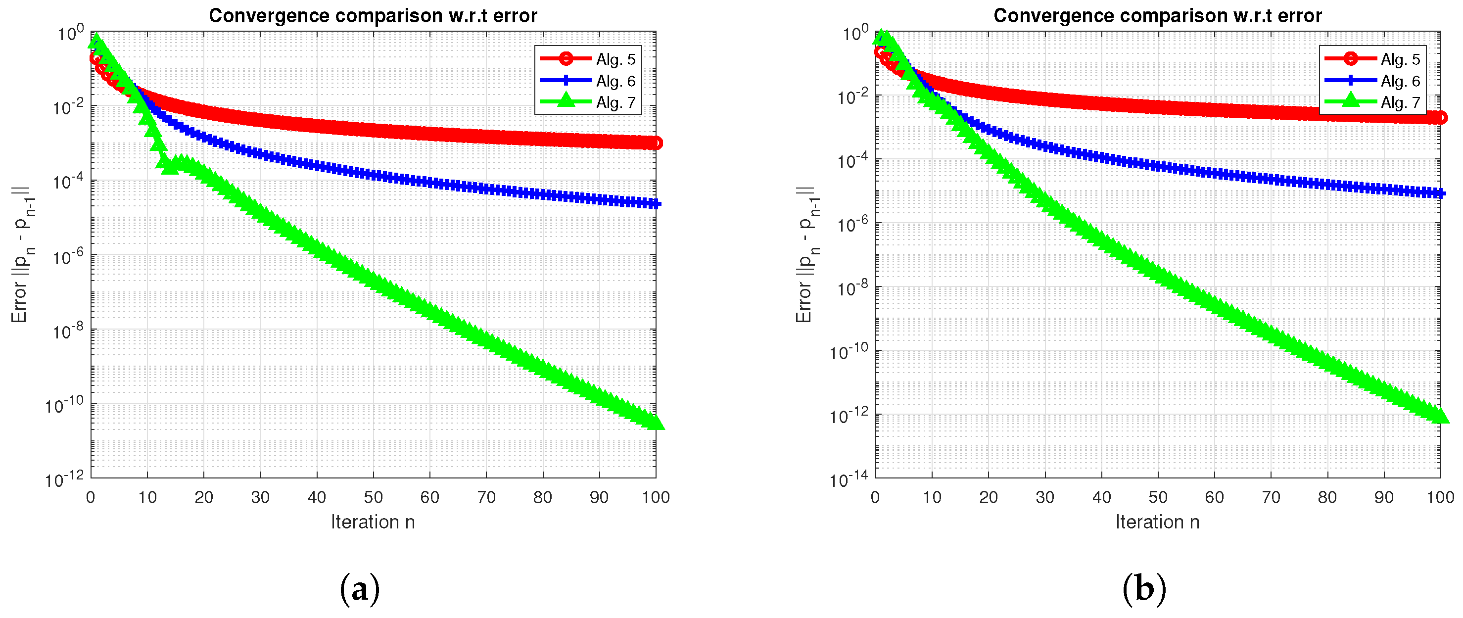
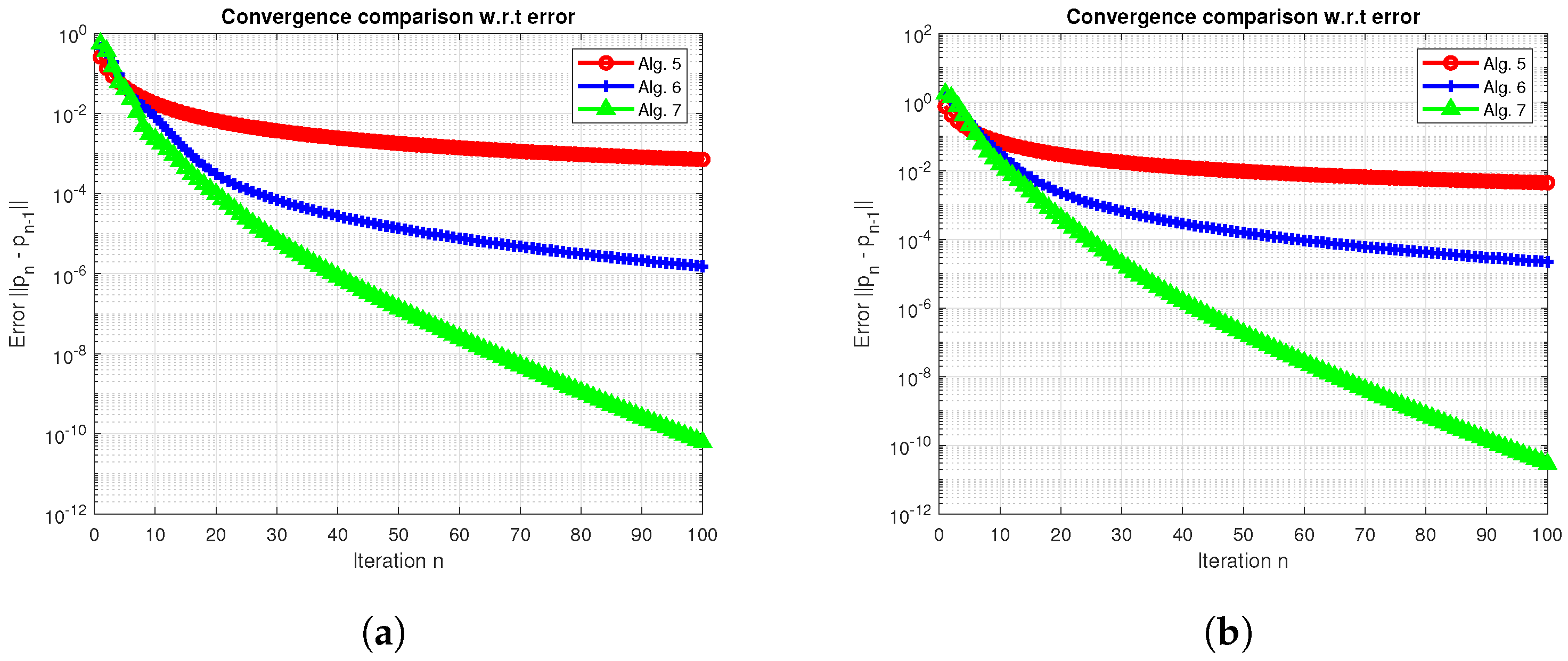
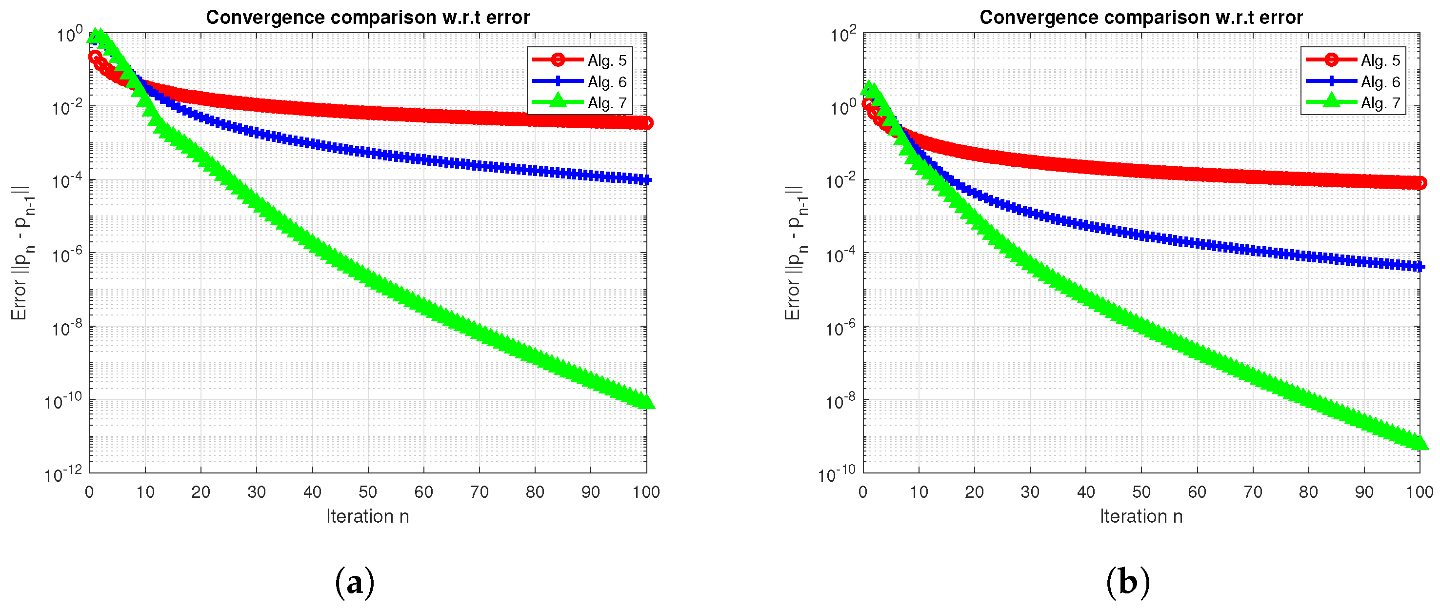
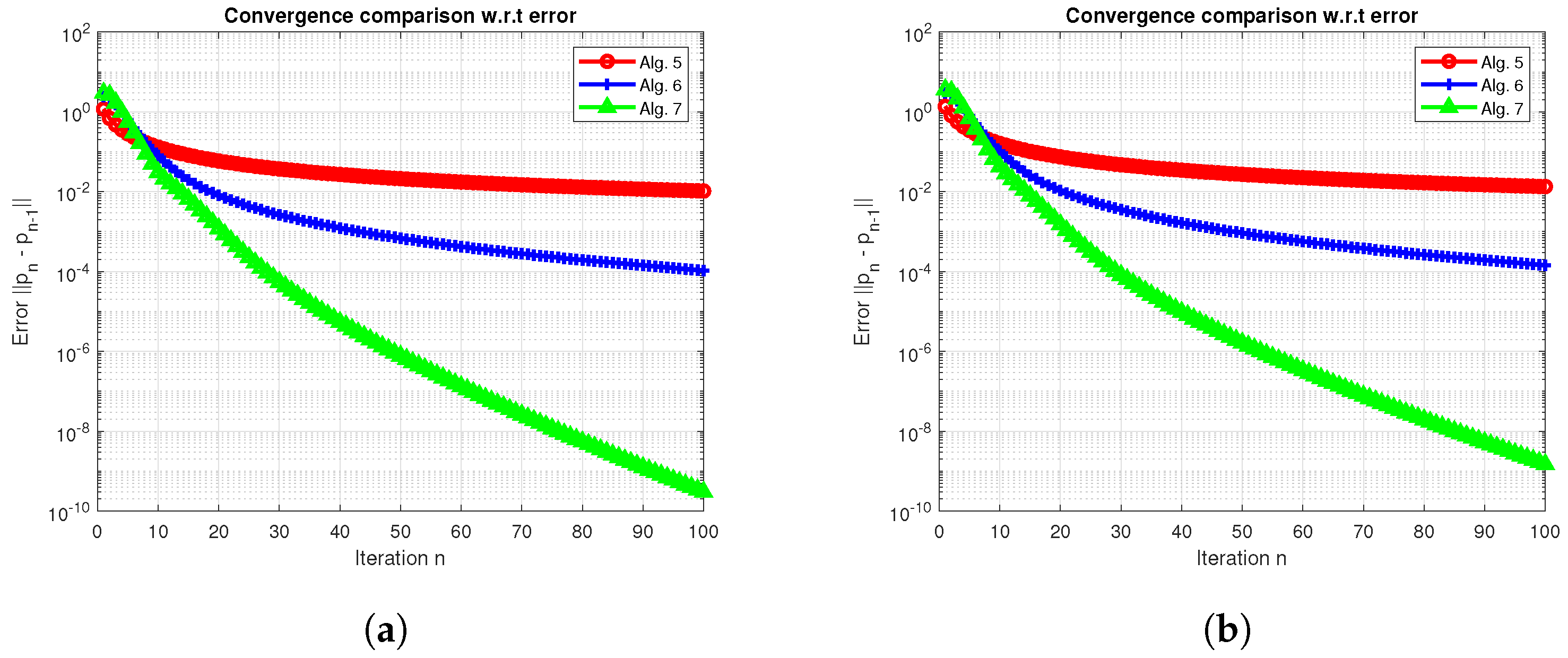
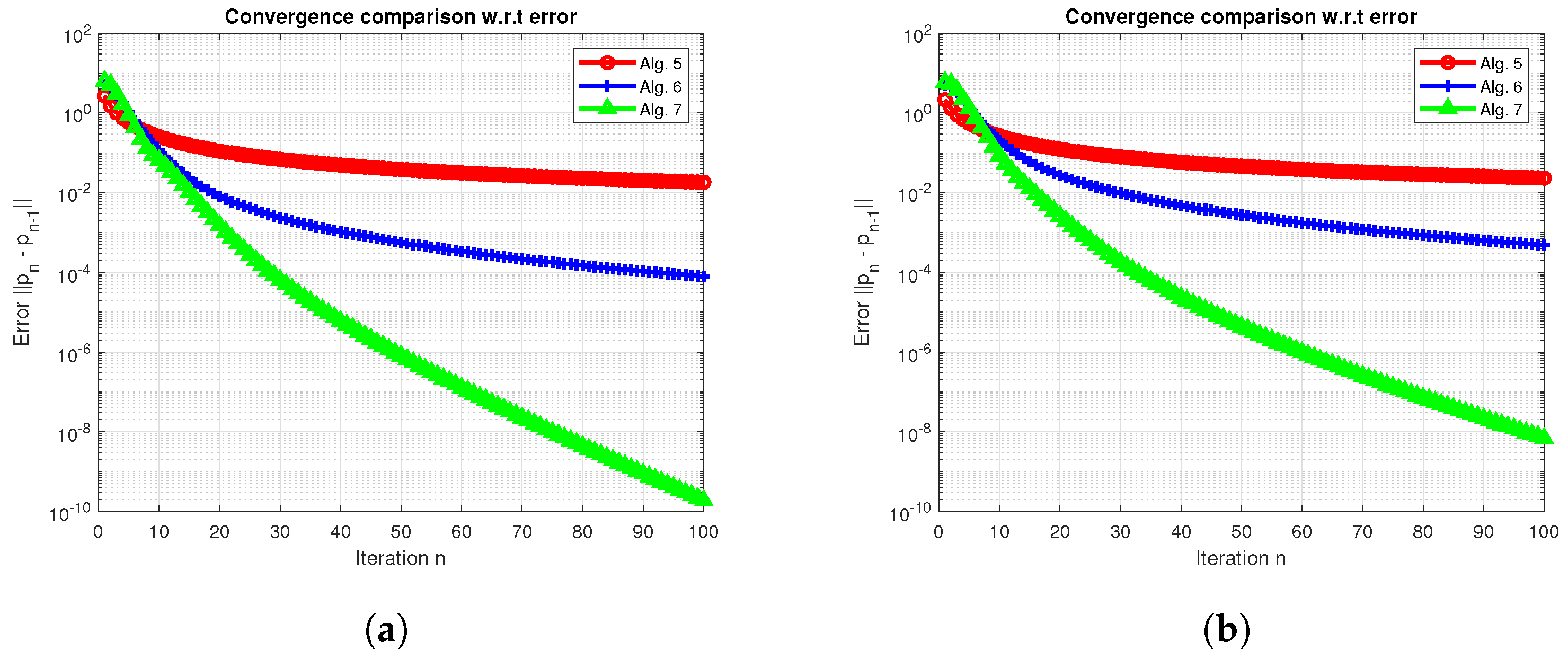
Further, we plot the error with the conditions and the comparable algorithms as given in Table 1, which shows the efficiency of our proposed algorithm and given in Figure 1, Figure 2, Figure 3, Figure 4 and Figure 5. We take the error comparison for 100 iterations during the illustrations.

Remark 6.

From Table 1, Table 2 and Table 3, it is observed that our proposed Algorithm 7 approximates the solution in fewer numbers of steps than Algorithms 5 and 6 and has less CPU time for different choices of $m,k,{\beta }_n$ and $k_n$ . Also, our proposed Algorithm 9 has a difference in the sense of the number of iterations and in the CPU time in the case of high-dimension spaces, for instance, for $(m,k)=(750,750)$ and $(m,k)=(2500,1100)$ . This shows the efficiency, reliability and effectiveness of Algorithm 7 when compared with Algorithms 5 and 6, which are in [29,30], respectively. Figure 1, Figure 2, Figure 3, Figure 4 and Figure 5 illustrate the error term for $n=1\to 100$ and also show that Algorithm 7 performs better than Algorithms 5 and 6; especially, it shows the big difference in the error terms during the convergence when the values of m and k are very high.

6. Image Restorations

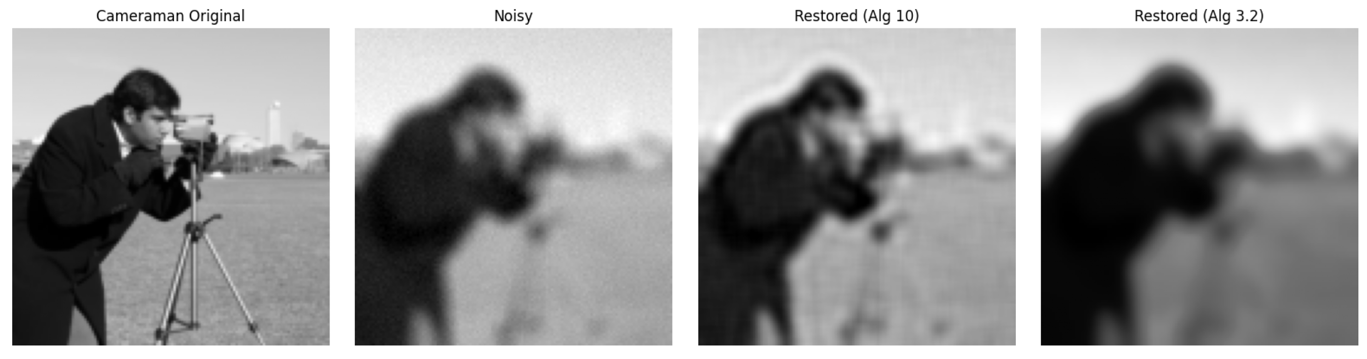
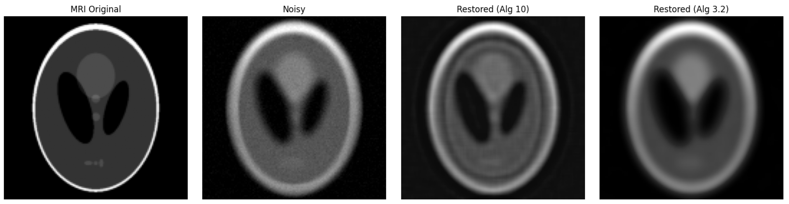
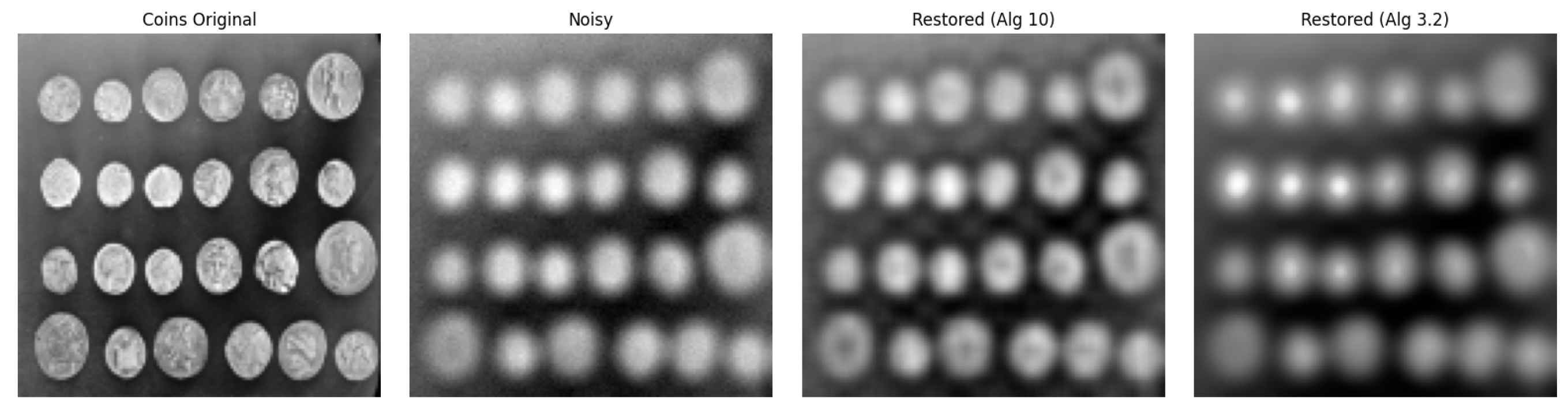
In the subsequent section, we applied our approach for the restoration of the image from the noisy one. We compared our proposed method with a recent method for the image restoration problem. For this purpose, we use the Python (version 3.12) as the programming language to compare Algorithm 10 with Algorithm 3.2 given in [39]. By recovering the images and comparing the CPU time and peak-signal-to-noise ratios, observe that our approach has good results compared to the other algorithm.

Now we discuss the following inverse problem from [53]:

$$Find{p}^{\ast }\in {\mathcal{H}}_1\mathrm{with}\mathrm{the}\mathrm{following},F\left(p^{\ast }\right)+M\left(p^{\ast }\right)=\underset{p\in {\mathcal{H}}_1}{\min }[F\left(p\right)+M\left(p\right)],\mathrm{and}L{p}^{\ast }\in F\left(S\right),$$

(81)

where L is a bounded linear operator form ${\mathcal{H}}_1$ to ${\mathcal{H}}_2$, $F:{\mathcal{H}}_1\to \mathbb{R}$ is convex and continuously differentiable, $M:{\mathcal{H}}_1\to \mathbb{R}$ is convex and lower semicontinuous, and S is any nonlinear self-mapping on ${\mathcal{H}}_2$. Further, let us recall a special case of (81) as the image restoration problem as follows:

$$\underset{p\in {\mathbb{R}}^n}{\min }{\{\parallel Dp-q\parallel }_2^2+{\eta \parallel p\parallel }_1\},$$

(82)

where $\eta >0$, $p\in {\mathbb{R}}^N$ is the original image, $q\in {\mathbb{R}}^M$ represents the observed noisy image, and the operator D from ${\mathbb{R}}^N$ onto ${\mathbb{R}}^M$ is linear. Here, $F\left(p\right)={\parallel Dp-q\parallel }_2^2$ and $M\left(p\right)={\eta \parallel p\parallel }_1$. Note that $\nabla F$ is continuous and monotone and $\partial M$ is maximal monotone. Hence, we have

$$F\left(p^{\ast }\right)+M\left(p^{\ast }\right)=\underset{p\in {\mathcal{H}}_1}{\min }[F\left(p\right)+M\left(p\right)]\iff 0\in (\nabla F\left(p^{\ast }\right)+\partial M\left(p^{\ast }\right)).$$

(83)

where $\nabla F$ is monotone and Lipschitzian with Lipschitz constant ${\parallel D\parallel }^2$.

If we set $G=0$, $F=\nabla F$, $P_{\mathcal{C}}=P_{\mathcal{C}}=I$, $M_1=M_2=\partial M$, and $S=T$ in our Algorithm 10, then the sequence $\left\{p_n\right\}$ thus obtained in Algorithm 10 approximates the solution of Equation (83).

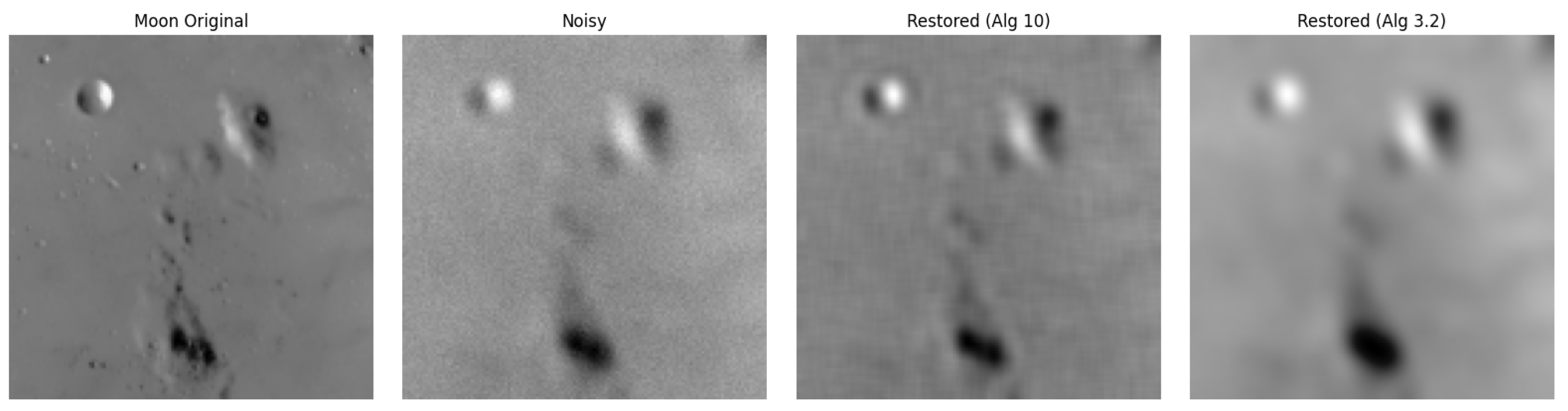
From the benchmark data set, we take $128\times 128$ images for cameraman, MRI, coins, and the moon. Further, we set standard deviation $\sigma =4$, Gaussian kernel size 9, ${\lambda }_n=\lambda =1.2$, ${\sigma }_n=\sigma =$, ${\gamma }_n=0.2$, ${\eta }_n=0.8$, ${\alpha }_n=0.5$ and maximum number of iterations 30 for our experiment. Moreover, we evaluate the performance of the algorithms by the quality of restored images with an evaluation matrix called the peak-signal-to-noise ratio (PSNR), measured in decibels (dB) and defined as follows:

$$\mathrm{PSNR}=10.{log}_{10}\left({\displaystyle \frac{{\mathrm{MAX}}^2}{\mathrm{MSE}}}\right),$$

where “MAX” indicates the maximum value of the pixel that the image can have and “MSE” is the mean squared error between the original $\left(p\right)$ and restored $\left(p^{\ast }\right)$ images. The higher PSNR values suggest superior restoration performance. The comparison results are given in Figure 6, Figure 7, Figure 8 and Figure 9 and in Table 4.

Table 4. Comparison of PSNR (dB) and CPU Time (s) for Algorithm 3.2 [39] and Algorithm 10.

Image	PSNR (Algorithm 3.2) [39]	Time (s)	PSNR (Algorithm 10)	Time (s)
Cameraman	28.26	2.31	28.93	1.49
MRI	25.80	2.20	26.42	1.38
Coins	26.52	2.15	27.14	1.33
Moon	27.77	2.23	28.38	1.41

Table 4. Comparison of PSNR (dB) and CPU Time (s) for Algorithm 3.2 [39] and Algorithm 10.

Image	PSNR (Algorithm 3.2) [39]	Time (s)	PSNR (Algorithm 10)	Time (s)
Cameraman	28.26	2.31	28.93	1.49
MRI	25.80	2.20	26.42	1.38
Coins	26.52	2.15	27.14	1.33
Moon	27.77	2.23	28.38	1.41

Remark 7.

Note that, Figure 6, Figure 7, Figure 8 and Figure 9 describe the original, blurred and restored images, which show that for different data sets, our proposed Algorithm 10 performs better for restoration of the images than the comparable algorithm given in [39]). Moreover, Table 4 shows the PSNR and the CPU time for 30 iterations for both algorithms; one can observe that our proposed approach is more efficient, as it has less CPU time and a higher value of PSNR for the restored image.

7. Conclusions and Future Directions

The problem of approximating the common solution of SVIP, SEP, SFP is studied in this paper in the context of Hilbert spaces. The main features of our paper are (1) a new extragradient algorithm with a self-adaptive step size is proposed for the solution of some nonlinear operator equations. (2) The strong convergence results for Algorithm 7 are proved. (3) A class of mappings discussed is more general than the class of mappings considered in [35,36]. (4) Solve certain problems having common solutions in contrast to the work in [29,30], and hence Theorem 1 of [30] and Theorem 3.2 of [29] are the special cases of our Theorem 1. (5) In the sense of rate of convergence, our proposed method is more efficient. (6) Further, based on our proposed method and our main result, Theorem 1, as applications, we find the solution of several nonlinear problems that are very useful in different disciplines of science and engineering. (7) We used our proposed approach for the image restoration problem. From Figure 6, Figure 7, Figure 8 and Figure 9, Table 4 and Remark 7, one can see our approach is more efficient while solving the image restoration problem than the comparable approach given in [39].

Several possible extensions of this work will be considered in the future. One direction is to extend the proposed algorithm from Hilbert spaces to Banach spaces, which requires different analytical tools. Another direction is to study more general mappings and bifunctions in order to broaden the applicability of the method. In addition, fully self-adaptive strategies for all control parameters will be explored to reduce manual tuning. Finally, the algorithm can be tested on larger data sets and applied to other practical problems such as signal processing and network optimization.

References

1. Bauschke, H.H.; Borwein, J.M. On projection algorithms for solving convex feasibility problems. SIAM Rev. 1996, 38, 367–426. [Google Scholar] [CrossRef] [Scilit]
2. Chen, P.; Huang, J.; Zhang, X. A primal-dual fixed point algorithm for convex separable minimization with applications to image restoration. Inverse Probl. 2013, 29, 025011. [Google Scholar] [CrossRef] [Scilit]
3. Goebel, K.; Reich, S. Uniform Convexity, Hyperbolic Geometry, and Non-Expansive Mappings; Marcel Dekker: New York, NY, USA; Basel, Switzerland, 1984. [Google Scholar]
4. Reich, S.; Shoikhet, D. Nonlinear Semigroups, Fixed Points, and Geometry of Domains in Banach Spaces; Imperial College Press: London, UK, 2005. [Google Scholar]
5. Deutsch, F. Best Approximation in Inner Product Spaces; Springer: Berlin/Heidelberg, Germany, 2001. [Google Scholar]
6. Ceng, L.C.; Petrusel, A.; Qin, X.; Yao, J.C. A modified inertial subgradient extragradient method for solving pseudomonotone variational inequalities and common fixed point problems. Fixed Point Theory 2020, 21, 93. [Google Scholar] [CrossRef] [Scilit]
7. Ceng, L.C. A subgradient-extragradient method for bilevel equilibrium problems with the constraints of variational inclusion systems and fixed point problems. Commun. Optim. Theory 2021, 2021, 4. [Google Scholar]
8. Liu, L.; Cho, S.Y.; Yao, J.C. Convergence analysis of an inertial Tsengs extragradient algorithm for solving pseudomonotone variational inequalities and applications. J. Nonlinear Var. Anal. 2021, 5, 627–644. [Google Scholar] [CrossRef] [Scilit]
9. Liu, L.; Yao, J.C. Iterative methods for solving variational inequality problems with a double-hierarchical structure in Hilbert spaces. Optimization 2023, 72, 2433–2461. [Google Scholar] [CrossRef] [Scilit]
10. Byrne, C. Iterative oblique projection onto convex sets and the split feasibility problem. Inverse Probl. 2002, 18, 441. [Google Scholar] [CrossRef] [Scilit]
11. Combettes, P.L. The convex feasibility problem in image recovery. Adv. Imaging Electron Phys. 1996, 95, 155–270. [Google Scholar]
12. Tang, Y. Convergence analysis of a new iterative algorithm for solving split variational inclusion problems. J. Ind. Manag. Optim. 2020, 16, 945. [Google Scholar] [CrossRef] [Scilit]
13. Censor, Y.; Gibali, A.; Reich, S. Algorithms for the split variational inequality problem. Numer. Algorithms 2012, 59, 301–323. [Google Scholar] [CrossRef] [Scilit]
14. Halpern, B. Fixed points of nonexpanding maps. Bull. Am. Math. Soc. 1967, 73, 957–961. [Google Scholar] [CrossRef] [Scilit]
15. Moudafi, A. Viscosity approximation methods for fixed-point problems. J. Math. Anal. Appl. 2000, 241, 46–55. [Google Scholar] [CrossRef] [Scilit]
16. Abbas, M.; Asghar, M.W.; De la Sen, M. Approximation of the solution of delay fractional differential equation using AA-iterative scheme. Mathematics 2022, 10, 273. [Google Scholar] [CrossRef] [Scilit]
17. Beg, I.; Abbas, M.; Asghar, M.W. Convergence of AA-iterative algorithm for generalized α-nonexpansive mappings with an application. Mathematics 2022, 10, 4375. [Google Scholar] [CrossRef] [Scilit]
18. Asghar, M.W.; Abbas, M.; Eyni, D.C.; Omaba, M.E. Iterative approximation of fixed points of generalized αm-nonexpansive mappings in modular spaces. AIMS Math. 2023, 8, 26922–26944. [Google Scholar] [CrossRef] [Scilit]
19. Abbas, M.; Ciobanescu, C.; Asghar, M.W.; Omame, A. Solution approximation of fractional boundary value problems and convergence analysis using AA-iterative scheme. AIMS Math. 2024, 9, 13129–13158. [Google Scholar] [CrossRef] [Scilit]
20. Suanoom, C.; Gebrie, A.G.; Grace, T. The convergence of AA-iterative algorithm for generalized AK-α-nonexpansive mappings in Banach spaces. Sci. Tech. Asia 2023, 28, 82–90. [Google Scholar]
21. Byrne, C.; Censor, Y.; Gibali, A.; Reich, S. The split common null point problem. J. Nonlinear Convex Anal. 2012, 13, 759–775. [Google Scholar]
22. Wangkeeree, R.; Rattanaseeha, K.; Wangkeeree, R. The general iterative methods for split variational inclusion problem and fixed point problem in Hilbert spaces. J. Comput. Anal. Appl. 2018, 25, 19. [Google Scholar]
23. Alakoya, T.O.; Mewomo, O.T. Viscosity S-iteration method with inertial technique and self-adaptive step size for split variational inclusion, equilibrium and fixed point problems. Comput. Appl. Math. 2022, 41, 39. [Google Scholar] [CrossRef] [Scilit]
24. Asghar, M.W.; Abbas, M.; Djafari-Rouhani, B. The AA-viscosity algorithm for fixed-point, generalized equilibrium and variational inclusion problems. Axioms 2024, 13, 38. [Google Scholar] [CrossRef] [Scilit]
25. Izuchukwu, C.; Ogwo, G.; Mewomo, O. An inertial method for solving generalized split feasibility problems over the solution set of monotone variational inclusions. Optimization 2022, 71, 583–611. [Google Scholar] [CrossRef] [Scilit]
26. Asghar, M.W.; Abbas, M. A self-adaptive viscosity algorithm for split fixed point problems and variational inequality problems in Banach spaces. J. Nonlinear Convex Anal. 2023, 24, 341–361. [Google Scholar]
27. Shehu, Y.; Iyiola, O.S.; Thong, D.V.; Van, N.T.C. An inertial subgradient extragradient algorithm extended to pseudomonotone equilibrium problems. Math. Methods Oper. Res. 2021, 93, 213–242. [Google Scholar] [CrossRef] [Scilit]
28. Alakoya, T.O.; Owolabi, A.; Mewomo, O.T. An inertial algorithm with a self-adaptive step size for a split equilibrium problem and a fixed point problem of an infinite family of strict pseudo-contractions. J. Nonlinear Var. Anal. 2021, 5, 803–829. [Google Scholar] [CrossRef] [Scilit]
29. Petrot, N.; Rabbani, M.; Khonchaliew, M.; Dadashi, V. A new extragradient algorithm for split equilibrium problems and fixed point problems. J. Inequal. Appl. 2019, 2019, 137. [Google Scholar] [CrossRef] [Scilit]
30. Ezeora, J.N.; Enyi, C.D.; Nwawuru, F.O.; Ogbonna, R.C. An algorithm for split equilibrium and fixed-point problems using inertial extragradient techniques. Comput. Appl. Math. 2023, 42, 103. [Google Scholar] [CrossRef] [Scilit]
31. Tan, B.; Chen, J.; Li, S.; Ou, X. Extragradient algorithms with double inertial for solving variational inequalities and applications to signal processing. Commun. Nonlinear Sci. Numer. Simul. 2025, 152, 109213. [Google Scholar] [CrossRef] [Scilit]
32. Ma, X.; Liu, H.; Li, X. Two optimization approaches for solving split variational inclusion problems with applications. J. Sci. Comput. 2022, 91, 58. [Google Scholar] [CrossRef] [Scilit]
33. Arfat, Y.; Kumam, P.; Ngiamsunthorn, P.S.; Khan, M.A.A.; Sarwar, H.; Fukhar-ud-Din, H. Approximation results for split equilibrium problems and fixed point problems of nonexpansive semigroup in Hilbert spaces. Adv. Differ. Equ. 2020, 2020, 512. [Google Scholar] [CrossRef] [Scilit]
34. Zhu, L.J.; Kuo, H.C.; Wen, C.F. Strong convergence results of split equilibrium problems and fixed point problems. J. Math. 2021, 2021, 6624321. [Google Scholar] [CrossRef] [Scilit]
35. Korpelevich, G.M. The extragradient method for finding saddle points and other problems. Matecon 1976, 12, 747–756. [Google Scholar]
36. Censor, Y.; Segal, A. The split common fixed point problem for directed operators. J. Convex Anal. 2009, 16, 587–600. [Google Scholar]
37. Luo, C.; Ji, H.; Li, Y. Utility-based multi-service bandwidth allocation in the 4G heterogeneous wireless access networks. In Proceedings of the 2009 IEEE Wireless Communications and Networking Conference, Budapest, Hungary, 5–8 April 2009; pp. 1–5. [Google Scholar]
38. Iiduka, H. Fixed point optimization algorithm and its application to network bandwidth allocation. J. Comput. Appl. Math. 2012, 236, 1733–1742. [Google Scholar] [CrossRef] [Scilit]
39. Godwin, E.C.; Izuchukwu, C.; Mewomo, O.T. Image restorations using a modified relaxed inertial technique for generalized split feasibility problems. Math. Methods Appl. Sci. 2023, 46, 5521–5544. [Google Scholar] [CrossRef] [Scilit]
40. Chuang, C.S. Strong convergence theorems for the split variational inclusion problem in Hilbert spaces. Fixed Point Theory Appl. 2013, 2013, 350. [Google Scholar] [CrossRef] [Scilit]
41. Mainge, P.E. Approximation methods for common fixed points of nonexpansive mappings in Hilbert spaces. J. Math. Anal. Appl. 2007, 325, 469–479. [Google Scholar] [CrossRef] [Scilit]
42. Goebel, K.; Kirk, W.A. Topics in Metric Fixed Point Theory; Cambridge University Press: Cambridge, UK, 1990. [Google Scholar]
43. Saejung, S.; Yotkaew, P. Approximation of zeros of inverse strongly monotone operators in Banach spaces. Nonlinear Anal. Theory Methods Appl. 2012, 75, 742–750. [Google Scholar] [CrossRef] [Scilit]
44. Mainge, P.E. Strong convergence of projected subgradient methods for nonsmooth and nonstrictly convex minimization. Set-Valued Anal. 2008, 16, 899–912. [Google Scholar] [CrossRef] [Scilit]
45. Aubin, J.P. Optima and Equilibria: An Introduction to Nonlinear Analysis; Springer Science & Business Media: Berlin/Heidelberg, Germany, 2002. [Google Scholar]
46. Anh, P.N. A hybrid extragradient method extended to fixed point problems and equilibrium problems. Optimization 2013, 62, 271–283. [Google Scholar] [CrossRef] [Scilit]
47. Moudafi, A.; Thakur, B.S. Solving proximal split feasibility problems without prior knowledge of operator norms. Opt. Lett. 2014, 8, 2099–2110. [Google Scholar] [CrossRef] [Scilit]
48. Abbas, M.; AlShahrani, M.; Ansari, Q.H.; Iyiola, O.S.; Shehu, Y. Iterative methods for solving proximal split minimization problems. Numer. Algorithms 2018, 78, 193–215. [Google Scholar] [CrossRef] [Scilit]
49. Censor, Y.; Elfving, T. A multiprojection algorithm using Bregman projections in a product space. Numer. Algorithms 1994, 8, 221–239. [Google Scholar] [CrossRef] [Scilit]
50. Padcharoen, A.; Kumam, P.; Chaipunya, P.; Shehu, Y. Convergence of inertial modified Krasnoselskii-Mann iteration with application to image recovery. Thai J. Math. 2020, 18, 126–141. [Google Scholar]
51. Nesterov, Y. A method for unconstrained convex minimization problem with the rate of convergence O(1/k2). Dokl. Akad. Nauk SSSR 1983, 269, 543. [Google Scholar]
52. Kazmi, K.R.; Rizvi, S.H. Iterative approximation of a common solution of a split equilibrium problem, a variational inequality problem and a fixed point problem. J. Egypt. Math. Soc. 2013, 21, 44–51. [Google Scholar] [CrossRef] [Scilit]
53. Beck, A.; Teboulle, M. A fast iterative shrinkage-thresholding algorithm for linear inverse problems. SIAM J. Imaging Sci. 2009, 2, 183–202. [Google Scholar] [CrossRef] [Scilit]
Figure 1. Comparisons of errors of Algorithm 7 with Algorithm 5 and Algorithm 6. (a) ( m , k ) = ( 3 , 3 ) , β n = 0.99 1 1 + n , (b) k n = 1 2 , ( m , k ) = ( 5 , 10 ) , β n = 0.99 1 1 + n , k n = 1 2 .
Mathematics 14 00652 g001
Figure 2. Comparisons of errors of Algorithm 7 with Algorithm 5 and Algorithm 6. (a) ( m , k ) = ( 10 , 5 ) , β n = 0.99 1 1 + n , k n = 1 2 , (b) ( m , k ) = ( 20 , 50 ) , β n = 0.99 1 1 + n , k n = 1 2 .
Mathematics 14 00652 g002
Figure 3. Comparisons of errors of Algorithm 7 with Algorithm 5 and Algorithm 6. (a) ( m , k ) = ( 50 , 20 ) , β n = 0.99 1 1 + n , k n = 1 2 , (b) ( m , k ) = ( 120 , 155 ) , β n = 0.99 1 1 + n , k n = 1 2 .
Mathematics 14 00652 g003
Figure 4. Comparisons of errors of Algorithm 7 with Algorithm 5 and Algorithm 6. (a) ( m , k ) = ( 310 , 220 ) , β n = 0.99 1 1 + n , k n = 1 2 , (b) ( m , k ) = ( 550 , 350 ) , β n = 0.99 1 1 + n , k n = 1 2 .
Mathematics 14 00652 g004
Figure 5. Comparisons of errors of Algorithm 7 with Algorithm 5 and Algorithm 6. (a) ( m , k ) = ( 750 , 750 ) , β n = 0.99 1 1 + n , k n = 1 2 , (b) ( m , k ) = ( 2500 , 1100 ) , β n = 0.99 1 1 + n , k n = 1 2 .
Mathematics 14 00652 g005
Figure 6. Comparison for cameraman.
Mathematics 14 00652 g006
Figure 7. Comparison for MRI.
Mathematics 14 00652 g007
Figure 8. Comparison for coins.
Mathematics 14 00652 g008
Figure 9. Comparison for moon.
Mathematics 14 00652 g009
Disclaimer/Publisher’s Note: The statements, opinions and data contained in all publications are solely those of the individual author(s) and contributor(s) and not of MDPI and/or the editor(s). MDPI and/or the editor(s) disclaim responsibility for any injury to people or property resulting from any ideas, methods, instructions or products referred to in the content.