Numerical Solutions via Shifted Pell Polynomials for Third-Order Rosenau–Hyman and Gilson–Pickering Equations

Abstract

This paper introduces a collocation algorithm for numerically solving the third-order Gilson–Pickering equation (GPE) and the classical Rosenau–Hyman equation (RHE). We employ newly developed shifted Pell polynomials as basis functions. Novel formulas for these polynomials are devised and utilized in constructing the proposed algorithm. Specifically, we establish a new power form and its inversion formula, along with an explicit formula for derivatives of the shifted Pell polynomials, from which the operational matrices of derivatives (OMDs) are derived. These matrices facilitate the conversion of nonlinear dispersive models into systems of algebraic equations, efficiently solved using Newton’s iterative technique. The error analysis of the shifted Pell expansion is discussed in depth. Several numerical examples, including the RHE, its fourth-order variant, and the Fornberg–Whitham equation, are provided to demonstrate the method’s performance and accuracy. Comparative results are also reported.

1. Introduction

Nonlinear differential equations (DEs) are important because they can model complex real-world events in many areas of the applied sciences. Studying nonlinear DEs can help us understand complex systems better. This is because nonlinear DEs can show a wide range of behaviors, unlike linear DEs. These behaviors encompass multistability, chaos, and bifurcations. Numerous models across several fields—including electrodynamics, neuroscience, epidemiology, and economics—can be represented using nonlinear DEs; see [1,2]. Given the importance of nonlinear models, numerous numerical methods have been developed to solve these equations, since analytical solutions are generally unavailable. The authors of [3] developed an efficient numerical scheme to solve numerically Korteweg–de Vries (KdV) equations, while in [4], a matrix approach was followed to solve the fifth-order KdV-type equations based on the shifted Horadam polynomials. The authors of [5] developed a two-step hybrid block scheme to handle the FitzHugh–Nagumo model. Regarding the numerical treatment of the nonlinear Kuramoto–Sivashinsky equation, the authors of [6] proposed a numerical method based on employing the quintic B-splines to solve it, while the authors of [7] adopted a fractional power-series technique to address the fractional Kawahara equations. In [8], an iterative finite-difference framework was designed to treat the nonlinear Gordon-type problems. For higher-order dispersive systems, the authors of [9] employed Schröder operational matrices to approximate solutions of the time-fractional generalized Kawahara equation, whereas the authors of [10] followed another numerical algorithm based on the eighth-kind Chebyshev operational matrices to treat the same classes of equations. The authors of [11] analyzed an advanced scheme for the nonlinear Schrödinger equation. In addition, in [12], the authors combined pseudo-spectral discretization with a variational quantum algorithm to numerically approximate nonlinear Schrödinger dynamics.

The special functions, including celebrated polynomials, are crucial due to their importance in various fields, such as mathematical physics, approximation theory, number theory, and numerical analysis. See, for example, [13,14]. In [15], a kind of generalized Chebyshev polynomial was utilized to analyze a collocation algorithm for treating the pantograph-type delay DEs. The study in [16] employed the third kind of Chebyshev polynomials to solve multi-term variable-order FDEs. In [17], the first-derivative Chebyshev polynomials were used along with a pseudo-Galerkin method to solve some specific DEs that arise in real-life applications. The work in [18] employed clique polynomials to handle the time-fractional Klein–Gordon equations. The suggested method presented in [19] incorporated new Fibonacci coefficient polynomials within a spectral collocation framework to solve the time-fractional Kuramoto–Sivashinsky equation. In [20], the polynomials, namely Vieta Lucas polynomials, were employed together with a non-standard finite difference scheme to solve some KdV equations. A matrix method was proposed to treat the fractional Burgers equations employing certain polynomials that generalize Fermat polynomials, while in [21], the authors used Pell coefficient polynomials within the Tau framework for hyperbolic partial DEs. The authors of [22] employed other shifted Vieta–Fibonacci polynomials to solve some fractional DEs. The study in [23] introduced novel Lucas coefficient polynomials and utilized them to treat two types of nonlinear equations. In [24], the authors demonstrated the use of Lucas polynomials to solve multidimensional Burgers-type equations.

Pell polynomials, which are particular polynomials of the so-called generalized Fibonacci polynomials, have attracted significant attention in numerical analysis. Many contributions have been made using these polynomials. For example, a matrix approach utilizing Pell polynomials was proposed to address the damped wave equation [25]. Pell polynomials have also been applied to solve certain fractional differential equations (FDEs) [26]. Furthermore, they have been utilized to obtain analytic and approximate solutions for other types of equations (FEs) [27]. A Pell polynomial-based method was developed within the Caputo–Fabrizio fractional derivative framework [28]. Furthermore, fractional-order Pell hybrid functions were introduced and applied to variable-order fractional differential equations [29].

Different spectral approaches are effective in handling different DEs. Many authors are interested in employing these methods to deal with different DEs. Their key benefit over more standard numerical approaches is that they can reach very high levels of accuracy for smooth problems through exponential or high-order convergence. These methods utilize unique functions or polynomials to provide accurate approximations with minimal degrees of freedom. Many areas have found practical applications for spectral methods, such as quantum physics, fluid dynamics, and modeling biological systems. For some instances of spectral methods in use, see [30,31]. There are three main spectral methods: collocation, tau, and Galerkin. Every method has its characteristics and advantages. The collocation approach is advantageous as it can be utilized for all types of DEs governed by any underlying conditions, as demonstrated in [32,33,34]. The Galerkin approach requires that the residual of the equations be orthogonal to the basis functions we have chosen; see, for instance, refs. [35,36]. The tau technique is more adaptable than the Galerkin method in selecting basis functions, as demonstrated in [37,38].

The utilization of different operational matrices of derivatives (OMDs) is useful in handling various types of DEs. They serve to reduce the DEs with their governing conditions into systems of algebraic equations that can be solved. Many authors used these matrices to treat DEs. For example, in [39], certain operational matrices were developed and used to treat some even-order partial DEs. The study in [40] utilized the operational matrix of Chebyshev polynomials to solve pantograph-type Volterra integro DEs. In [41], harmonic numbers operational matrices of derivatives were established and used to treat linear and nonlinear sixth-order two-point BVPs. Another operational approach using Genocchi polynomials was followed in [42] to solve some delay DEs. The proposed method in [43] used Bernstein polynomials and their operational matrices to handle population models. The study in [44] developed operational matrices based on fractional -order Lagrange polynomials to solve space–time fractional partial DEs. In [45], the OMDs of the Chebyshev polynomials were used to treat the Lane–Emden equations.

The main aim of the current paper is to develop a spectral collocation method for solving the third-order GPE and the classical Rosenau–Hyman equation (RHE). The shifted Pell polynomials are introduced and used as basis functions.

The paper is organized as follows. Section 2 presents an account of the well-known Pell polynomials. Also, certain shifted Pell polynomials are introduced in this section. Section 3 develops some new formulas of the shifted Pell polynomials, which will be important to design the proposed numerical algorithms. A collocation scheme is analyzed in Section 4 to solve the third-order Gilson–Pickering equation. Another collocation procedure is analyzed in Section 5 to handle the classical Rosenau–Hyman equation. The convergence and error bound are investigated in Section 6. Some numerical experiments are presented in Section 7. Finally, Section 8 reports some remarks.

2. An Overview of Pell Polynomials and Their Shifted Polynomials

This section presents an account of Pell polynomials and some of their characteristics. The Pell polynomials $P_n\left(x\right)$ are generalizations of the Pell numbers that are satisfied by the following recurrence relation:

$$P_{n+1}=2P_n+P_{n-1},P_0\left(x\right)=0,P_1\left(x\right)=1,n\ge 1.$$

(1)

The first few Pell numbers are 0, 1, 2, 5, 12, 29, 70, 169, ….

The Pell polynomials can be generated with the aid of the following recursive formula:

$$P_{n+1}\left(x\right)=2x{P}_n\left(x\right)+P_{n-1}\left(x\right),P_0\left(x\right)=0,P_1\left(x\right)=1,n\ge 1.$$

(2)

In addition, they can be represented using Binet’s form as

$$P_n\left(x\right)={\displaystyle \frac{{(x+\sqrt{x^2+1})}^n-{(x-\sqrt{x^2+1})}^n}{2\sqrt{x^2+1}}}.$$

(3)

Also, the following generating function may generate these polynomials

$$\sum _{n=0}^{\infty }{P}_n\left(x\right)t^n={\displaystyle \frac{t}{1-2xt-t^2}}.$$

(4)

The power series representation for these polynomials is

$$P_i\left(x\right)=\sum _{m=0}^{\lfloor i/2\rfloor }{\displaystyle \frac{2^{i-2m}(i-m)!}{m!(i-2m)!}}{x}^{i-2m},$$

(5)

while $x^m$ can be expanded in terms of $P_i\left(x\right)$ as

$$x^m=\sum _{i=0}^{\lfloor m/2\rfloor }{\displaystyle \frac{{(-1)}^i(m-2i+1)m!}{i!2^m(m-i+1)!}}{P}_{m-2i}\left(x\right).$$

(6)

It is useful to introduce the shifted Pell polynomials defined as

$$P_i^{*}\left(x\right)=P_i(2x-1).$$

(7)

In the following section, we develop some new useful formulas of the shifted Pell polynomials, which serve in the analysis of the proposed numerical algorithm.

3. Some New Important Formulas Concerned with the Shifted Pell Polynomials

In this section, we are interested in developing some new formulas for the shifted Pell polynomials, which are required to design our numerical algorithms in the upcoming sections.

Theorem 1.

For a positive integer i, the following power form representation of $P_i^{*}\left(x\right)$ holds:

$$P_i^{*}\left(x\right)=\sum _{s=0}^i{2}^{i+s}{(-1)}^{i+s}\left({\displaystyle \genfrac{}{}{0pt}{}{i}{s}}\right){}_{2}F_1\left(\begin{array}{c}{\displaystyle \frac{s-i}{2}},{\displaystyle \frac{-i+s+1}{2}}\\ -i\end{array}{\displaystyle |}-1\right)x^s.$$

(8)

Proof. 

Based on the analytic form of the Pell polynomials, one can write the following representation for the corresponding shifted polynomials, replacing x by $(2x-1)$:

$$P_i^{*}\left(x\right)=\sum _{k=0}^{\lfloor i/2\rfloor }{2}^{i-2k}\left({\displaystyle \genfrac{}{}{0pt}{}{i-k}{k}}\right){(2x-1)}^{i-2k}.$$

(9)

Expanding the last expression using the binomial theorem gives

$$P_i^{*}\left(x\right)=\sum _{k=0}^{\lfloor i/2\rfloor }{2}^{i-2k}\left({\displaystyle \genfrac{}{}{0pt}{}{i-k}{k}}\right)\sum _{r=0}^{i-2k}{(-1)}^i\left({\displaystyle \genfrac{}{}{0pt}{}{i-2k}{r}}\right){(-2)}^r{x}^r.$$

(10)

The last formula can be written alternatively in the form

$$P_i^{*}\left(x\right)=\sum _{s=0}^i\sum _{L=0}^{\lfloor i/2\rfloor }{(-1)}^{i+s}{2}^{i-2L+s}\left({\displaystyle \genfrac{}{}{0pt}{}{i-2L}{s}}\right)\left({\displaystyle \genfrac{}{}{0pt}{}{i-L}{L}}\right)x^s,$$

(11)

which can also be written as

$$P_i^{*}\left(x\right)=\sum _{s=0}^i{2}^{i+s}{(-1)}^{i+s}\left({\displaystyle \genfrac{}{}{0pt}{}{i}{s}}\right){}_{2}F_1\left(\begin{array}{c}{\displaystyle \frac{s-i}{2}},{\displaystyle \frac{-i+s+1}{2}}\\ -i\end{array}|-1\right)x^s.$$

(12)

This proves (8). □

Theorem 2.

The inversion formula of $P_i^{*}\left(x\right)$ is

$$x^r=\sum _{L=0}^r{H}_{L,r}{P}_L^{*}\left(x\right),$$

(13)

where

$$\begin{array}{cc}\hfill & H_{L,j}=(L+1)j!4^{-j}\hfill \\ \hfill & \times \left\{\begin{array}{cc}{\displaystyle \frac{{(-1)}^{\frac{(j-L)}{2}}}{\left(\frac{j-L}{2}\right)!\left(\frac{j+L+2}{2}\right)!}{}_{2}F_1\left(\begin{array}{c}-\frac{1}{2}(j+L+2),\frac{1}{2}(L-j)\\ \frac{1}{2}\end{array}|-1\right),}\hfill & (j-L)\mathit{even},\hfill \\ {\displaystyle \frac{2{(-1)}^{\frac{(j-L)+3}{2}}}{\left(\frac{j-L-1}{2}\right)!\left(\frac{j+L+1}{2}\right)!}{}_{2}F_1\left(\begin{array}{c}-\frac{1}{2}(j+L+1),\frac{1}{2}(-j+L+1)\\ \frac{3}{2}\end{array}|-1\right),}\hfill & (j-L)\mathit{odd}.\hfill \end{array}\right.\hfill \end{array}$$

(14)

Proof. 

It is more convenient to prove the alternative form of (13), written as

$$x^r=\sum _{m=0}^{\lfloor r/2\rfloor }{G}_{m,r}{P}_{r-2m}^{*}+\sum _{m=0}^{\lfloor (r-1)/2\rfloor }{R}_{m,r}{P}_{r-2m-1}^{*},$$

(15)

where

$$\begin{array}{cc}\hfill G_{m,r}& ={\displaystyle \frac{{(-1)}^{m+1}{2}^{-r}(-1-r+2m)2^{-r}r!}{m!(r-m+1)!}}{}_{2}F_1\left(\begin{array}{c}-m,-1-r+m\\ \frac{1}{2}\end{array}|-1\right),\hfill \end{array}$$

(16)

$$\begin{array}{cc}\hfill R_{m,r}& ={\displaystyle \frac{{(-1)}^{m+1}{2}^{-r}(-r+2m)2^{1-r}r!}{m!(r-m)!}}{}_{2}F_1\left(\begin{array}{c}-m,-r+m\\ \frac{3}{2}\end{array}|-1\right).\hfill \end{array}$$

(17)

We proceed by induction on r. The formula is correct at $r=0$. Assume that (15) holds, and we will prove the following formula:

$$x^{r+1}=\sum _{m=0}^{\lfloor (r+1)/2\rfloor }{G}_{m,r+1}{P}_{r-2m+1}^{*}\left(x\right)+\sum _{m=0}^{\lfloor r/2\rfloor }{R}_{m,r+1}{P}_{r-2m}^{*}\left(x\right).$$

(18)

The last formula can be split into

$$\begin{array}{cc}\hfill x^{2r+1}& =\sum _{m=0}^r{G}_{m,2r+1}{P}_{2r-2m+1}^{*}\left(x\right)+\sum _{m=0}^r{R}_{m,2r+1}{P}_{2r-2m}^{*}\left(x\right),\hfill \end{array}$$

(19)

$$\begin{array}{cc}\hfill x^{2r}& =\sum _{m=0}^r{G}_{m,2r}{P}_{2r-2m}^{*}\left(x\right)+\sum _{m=0}^r{R}_{m,2r}{P}_{2r-2m-1}^{*}\left(x\right).\hfill \end{array}$$

(20)

The proofs of (19) and (20) are similar; we prove (19).

• Multiplying the valid formula (15) by x, along with the application of the recurrence relation for the Pell polynomials in the form

$$x{P}_n\left(x\right)=\frac{1}{2}\left(P_{n+1}\left(x\right)-P_{n-1}\left(x\right)\right),$$

(21)

we get

$$\begin{array}{cc}\hfill x^{r+1}& =\sum _{m=0}^{\lfloor r/2\rfloor }{G}_{m,r}\left(\frac{1}{4}{P}_{r-2m+1}^{*}\left(x\right)+\frac{1}{2}{P}_{r-2m}^{*}\left(x\right)-\frac{1}{4}{P}_{r-2m-1}^{*}\left(x\right)\right)\hfill \\ \hfill & +\sum _{m=0}^{\lfloor (r-1)/2\rfloor }{R}_{m,r}\left(\frac{1}{4}{P}_{r-2m}^{*}\left(x\right)+\frac{1}{2}{P}_{r-2m-1}^{*}\left(x\right)-\frac{1}{4}{P}_{r-2m-2}^{*}\left(x\right)\right).\hfill \end{array}$$

(22)

If r is replaced by $2r$, then we get

$$\begin{array}{cc}\hfill x^{2r+1}& =\sum _{m=0}^r{G}_{m,2r}\left(\frac{1}{4}{P}_{2r-2m+1}^{*}\left(x\right)+\frac{1}{2}{P}_{2r-2m}^{*}\left(x\right)-\frac{1}{4}{P}_{2r-2m-1}^{*}\left(x\right)\right)\hfill \\ \hfill & +\sum _{m=0}^{r-1}{R}_{m,2r}\left(\frac{1}{4}{P}_{2r-2m}^{*}\left(x\right)+\frac{1}{2}{P}_{2r-2m-1}^{*}\left(x\right)-\frac{1}{4}{P}_{2r-2m-2}^{*}\left(x\right)\right),\hfill \end{array}$$

(23)

which can be written after some algebraic computations into the following form:

$$x^{2r+1}=\sum _{m=0}^r{Z}_{m,r}{P}_{2r-2m}^{*}\left(x\right)+\sum _{m=0}^r{\overline{Z}}_{m,r}{P}_{2r-2m+1}^{*}\left(x\right),$$

(24)

where

$$\begin{array}{cc}\hfill Z_{m,r}& =\frac{1}{2}{G}_{m,2r}+\frac{1}{4}{R}_{m,2r}-\frac{1}{4}{R}_{m-1,2r},\hfill \end{array}$$

(25)

$$\begin{array}{cc}\hfill {\overline{Z}}_{m,r}& =\frac{1}{4}{G}_{m,2r}-\frac{1}{4}{G}_{m-1,2r}+\frac{1}{2}{R}_{m-1,2r}.\hfill \end{array}$$

(26)

Some lengthy algebraic manipulations lead to the following relations:

$$\begin{array}{cc}\hfill R_{m,2r+1}& =Z_{m,r},\hfill \end{array}$$

(27)

$$\begin{array}{cc}\hfill G_{m,2r+1}& ={\overline{Z}}_{m,r}.\hfill \end{array}$$

(28)

Hence, Formula (19) follows, and (20) can be proved similarly. □

Theorem 3.

Consider two positive integers $i,q$ with $i\ge q$. We have

$${\displaystyle \frac{d^q{P}_i^{*}\left(x\right)}{d{x}^q}}=\sum _{s=0}^{i-q}{\overline{U}}_{s,i,q}{P}_s^{*}\left(x\right),$$

(29)

where

$${\overline{U}}_{s,i,q}={\lambda }_{s,i,q}{\displaystyle \frac{{(-1)}^{\frac{i-s-q}{2}}{2}^{2q}(s+1)\left(\frac{1}{2}(-2+i-s+q)\right)!\left(\frac{1}{2}(i+s+q)\right)!}{\left(\frac{1}{2}(i-s-q)\right)!\left(\frac{1}{2}(2+i+s-q)\right)!(q-1)!}},$$

(30)

and

$${\lambda }_{s,i,q}=\left\{\begin{array}{cc}1,\hfill & (i+s+q)\mathit{even},\hfill \\ 0,\hfill & \mathit{otherwise}.\hfill \end{array}\right.$$

Proof. 

First, we prove the derivative formula for the standard Pell polynomials, then find the corresponding derivative formula for their shifted forms. Now, we will derive a derivative formula for Pell polynomials in the form

$${\displaystyle \frac{d^q{P}_i\left(x\right)}{d{x}^q}}=\sum _{s=0}^{i-q}{U}_{s,i,q}{P}_s\left(x\right),$$

(31)

and the coefficients $U_{s,i,q}$ will be explicitly determined.

• Using the power form representation of the Pell polynomials in (5), we obtain

$${\displaystyle \frac{d^q{P}_i\left(x\right)}{d{x}^q}}=\sum _{r=0}^{\lfloor \frac{i-q}{2}\rfloor }{\displaystyle \frac{2^{i-2r}(i-r)!}{(i-q-2r)!r!}}{x}^{i-2r-q}.$$

(32)

If the inversion Formula (6) is utilized, then (32) turns into

$$\begin{array}{cc}\hfill {\displaystyle \frac{d^q{P}_i\left(x\right)}{d{x}^q}}& =\sum _{r=0}^{\lfloor \frac{i-q}{2}\rfloor }{\displaystyle \frac{2^{i-2r}(i-r)!}{(i-q-2r)!r!}}\sum _{t=0}^{\lfloor \frac{i-q}{2}\rfloor -r}{\displaystyle \frac{{(-1)}^t{2}^{-i+q+2r}(1+i-q-2r-2t)(i-q-2r)!}{(1+i-q-2r-t)!t!}}\times \hfill \\ \hfill & P_{i-q-2r-2t}\left(x\right).\hfill \end{array}$$

(33)

Rearranging the terms yields the following formula:

$${\displaystyle \frac{d^q{P}_i\left(x\right)}{d{x}^q}}=2^q\sum _{s=0}^{\lfloor \frac{i-q}{2}\rfloor }(-1-i+2s+q)\sum _{r=0}^s{\displaystyle \frac{{(-1)}^{1+s-r}(i-r)!}{(s-r)!r!(i-s-q-r+1)!}}{P}_{i-q-2s}\left(x\right).$$

(34)

Formula (34) can be written in terms of ${}_{2}F_1\left(1\right)$ as

$${\displaystyle \frac{d^q{P}_i\left(x\right)}{d{x}^q}}=2^{q}i!\sum _{s=0}^{\lfloor \frac{i-q}{2}\rfloor }{\displaystyle \frac{{(-1)}^{1+s}(-1-i+2s+q)}{s!(1+i-s-q)!}}{}_{2}F_1\left(\begin{array}{c}-s,-1-i+s+q\\ -i\end{array}|1\right)P_{i-q-2s}\left(x\right).$$

(35)

Chu–Vandermonde’s identity [46] can be used to reduce (35) into the form

$${\displaystyle \frac{d^q{P}_i\left(x\right)}{d{x}^q}}=2^{q}i!\sum _{s=0}^{\lfloor \frac{i-q}{2}\rfloor }{\displaystyle \frac{{(-1)}^{1+s}(-1-i+2s+q)(i-s)!(s+q-1)!}{i!s!(1+i-s-q)!(q-1)!}}{P}_{i-q-2s}\left(x\right),$$

(36)

which is equivalent to

$${\displaystyle \frac{d^q{P}_i\left(x\right)}{d{x}^q}}=\sum _{s=0}^{i-q}{\lambda }_{s,i,q}{\displaystyle \frac{i^{i-s-q}{2}^q(s+1)\left(\frac{1}{2}(-2+i-s+q)\right)!\left(\frac{1}{2}(i+s+q)\right)!}{\left(\frac{1}{2}(i-s-q)\right)!\left(\frac{1}{2}(2+i+s-q)\right)!(q-1)!}}{P}_s\left(x\right).$$

(37)

The last formula can be written in the form of (31), with $U_{s,i,q}$ given by

$$U_{s,i,q}={\lambda }_{s,i,q}{\displaystyle \frac{{(-1)}^{\frac{i-s-q}{2}}{2}^q(s+1)\left(\frac{1}{2}(-2+i-s+q)\right)!\left(\frac{1}{2}(i+s+q)\right)!}{\left(\frac{1}{2}(i-s-q)\right)!\left(\frac{1}{2}(2+i+s-q)\right)!(q-1)!}}.$$

(38)

Finally, replacing x by $(2x-1)$ gives the corresponding derivative formula for the shifted Pell polynomials:

$${\displaystyle \frac{d^q{P}_i^{*}\left(x\right)}{d{x}^q}}=\sum _{s=0}^{i-q}{\overline{U}}_{s,i,q}{P}_s^{*}\left(x\right),$$

(39)

where ${\overline{U}}_{s,i,q}$ are given by

$${\overline{U}}_{s,i,q}=2^q{U}_{s,i,q}.$$

(40)

This completes the proof. □

Corollary 1.

The following derivative formulas of $P_i^{*}\left(x\right)$ are valid:

$$\begin{array}{cc}\hfill & {\displaystyle \frac{d{P}_i^{*}\left(x\right)}{dx}}=\sum _{s=0}^{i-1}{\mathcal{A}}_{s,i}^1{P}_s^{*}\left(x\right),i\ge 1,\hfill \end{array}$$

(41)

$$\begin{array}{cc}\hfill & {\displaystyle \frac{d^2{P}_i^{*}\left(x\right)}{d{x}^2}}=\sum _{s=0}^{i-2}{\mathcal{A}}_{s,i}^2{P}_s^{*}\left(x\right),i\ge 2,\hfill \end{array}$$

(42)

$$\begin{array}{cc}\hfill & {\displaystyle \frac{d^3{P}_i^{*}\left(x\right)}{d{x}^3}}=\sum _{s=0}^{i-3}{\mathcal{A}}_{s,i}^3{P}_s^{*}\left(x\right),i\ge 3,\hfill \end{array}$$

(43)

where ${\mathcal{A}}_{s,i}^1={\overline{U}}_{s,i,1}$, ${\mathcal{A}}_{s,i}^2={\overline{U}}_{s,i,2}$, and ${\mathcal{A}}_{s,i}^3={\overline{U}}_{s,i,3}$.

Proof. 

The proof of Corollary 1 can be easily obtained by substituting $q=1,2,3$ in Theorem 3. □

Remark 1.

Consider the following vector:

$${\mathit{P}}^{*}\left(\sigma \right)={[P_0^{*}\left(\sigma \right),P_1^{*}\left(\sigma \right),\dots ,P_{\mathcal{J}}^{*}\left(\sigma \right)]}^T.$$

(44)

The derivatives in Corollary 1 for the vector ${\mathit{P}}^{*}\left(\sigma \right)$ can be expressed, respectively, as

$$\begin{array}{cc}\hfill & {\displaystyle \frac{d{\mathit{P}}^{*}\left(\sigma \right)}{d\sigma }}=\mathit{A}{\mathit{P}}^{*}\left(\sigma \right),\hfill \\ & {\displaystyle \frac{d^2{\mathit{P}}^{*}\left(\sigma \right)}{d{\sigma }^2}}=\mathit{B}{\mathit{P}}^{*}\left(\sigma \right),\hfill \\ & {\displaystyle \frac{d^3{\mathit{P}}^{*}\left(\sigma \right)}{d{\sigma }^3}}=\mathit{F}{\mathit{P}}^{*}\left(\sigma \right),\hfill \end{array}$$

(45)

where $\mathit{A}=\left({\mathcal{A}}_{s,i}^1\right)$, $\mathit{B}=\left({\mathcal{A}}_{s,i}^2\right)$, and $\mathit{F}=\left({\mathcal{A}}_{s,i}^3\right)$, are the operational matrices of derivatives of order ${(\mathcal{J}+1)}^2$.

4. A Collocation Method for the Third-Order Gilson–Pickering Equation

Consider the following third-order Gilson-Pickering equation (GPE):

$${\mathcal{Z}}_t-\nu {\mathcal{Z}}_{\sigma \sigma t}+2\kappa {\mathcal{Z}}_{\sigma }-\mathcal{Z}{\mathcal{Z}}_{3\sigma }-\delta \mathcal{Z}{\mathcal{Z}}_{\sigma }-\zeta {\mathcal{Z}}_{\sigma }{\mathcal{Z}}_{\sigma \sigma }=0,0\le \sigma ,t\le 1.$$

(46)

equipped with the following conditions:

$$\begin{array}{cc}\hfill \mathcal{Z}(\sigma ,0)& =f\left(\sigma \right),\hfill \\ \hfill \mathcal{Z}(0,t)& =g_1\left(t\right),{\mathcal{Z}}_{\sigma }(0,t)=g_2\left(t\right),\hfill \\ \hfill \mathcal{Z}(1,t)& =g_3\left(t\right),{\mathcal{Z}}_{\sigma }(1,t)=g_4\left(t\right).\hfill \end{array}$$

(47)

where $f\left(\sigma \right),g_1\left(t\right),g_2\left(t\right),g_3\left(t\right)$ and $g_4\left(t\right)$ are differentiable functions.

Remark 2.

We want to mention the following important points:

• Gilson and Pickering [47] first proposed the GPE, which has no specific initial or boundary conditions.
• The formulation of the initial and boundary conditions used in this study follows Akbar et al. [48].
• While four conditions are listed, only three are independent spatial boundary conditions. The remaining condition is a compatibility condition.

Remark 3.

The Rosenau–Hyman equation (RHE) and the Fornberg–Whitham equation (FWE) are special cases of the GPE, introduced by Gilson and Pickering [47], given by the following.

• When $\nu =\kappa =0$, $\delta =1$ and $\zeta =3$, we obtain an RHE equation of the form

  $${\mathcal{Z}}_t-\mathcal{Z}{\mathcal{Z}}_{3\sigma }-\mathcal{Z}{\mathcal{Z}}_{\sigma }-3{\mathcal{Z}}_{\sigma }{\mathcal{Z}}_{\sigma \sigma }=0.$$

  (48)
• When $\nu =1$, $\kappa ={\displaystyle \frac{1}{2}}$, $\delta =-1$ and $\zeta =3$, we have an FWE equation of the form

  $${\mathcal{Z}}_t-{\mathcal{Z}}_{\sigma \sigma t}+{\mathcal{Z}}_{\sigma }-\mathcal{Z}{\mathcal{Z}}_{3\sigma }+\mathcal{Z}{\mathcal{Z}}_{\sigma }-3{\mathcal{Z}}_{\sigma }{\mathcal{Z}}_{\sigma \sigma }=0,$$

  (49)

Now, define the following space function:

$${\mathcal{Q}}^{\mathcal{J}}=\mathrm{span}\{P_m^{*}\left(\sigma \right)P_n^{*}\left(t\right):0\le m,n\le \mathcal{J}\},$$

(50)

then any function ${\mathcal{Z}}^{\mathcal{J}}={\mathcal{Z}}^{\mathcal{J}}(\sigma ,t)\in {\mathcal{Q}}^{\mathcal{J}}$ can be represented as

$${\mathcal{Z}}^{\mathcal{J}}=\sum _{m=0}^{\mathcal{J}}\sum _{n=0}^{\mathcal{J}}{\widehat{z}}_{mn}{P}_m^{*}\left(\sigma \right)P_n^{*}\left(t\right)={\mathit{P}}^{*}{\left(\sigma \right)}^T\widehat{\mathit{Z}}{\mathit{P}}^{*}\left(t\right),$$

(51)

where, ${\mathit{P}}^{*}\left(\sigma \right)={[P_0^{*}\left(\sigma \right),P_1^{*}\left(\sigma \right),\dots ,P_{\mathcal{J}}^{*}\left(\sigma \right)]}^T,{\mathit{P}}^{*}\left(t\right)={[P_0^{*}\left(t\right),P_1^{*}\left(t\right),\dots ,P_{\mathcal{J}}^{*}\left(t\right)]}^T,$ and $\widehat{\mathit{Z}}={\left({\widehat{z}}_{mn}\right)}_{0\le m,n\le \mathcal{J}}$ is the unknown matrix of order ${(\mathcal{J}+1)}^2$.

• Now, the residual ${\mathbf{R}}_1(\sigma ,t)$ of Equation (46) can be written as

$${\mathbf{R}}_1(\sigma ,t)={\mathcal{Z}}_t^{\mathcal{J}}-\nu {\mathcal{Z}}_{\sigma \sigma t}^{\mathcal{J}}+2\kappa {\mathcal{Z}}_{\sigma }^{\mathcal{J}}-{\mathcal{Z}}^{\mathcal{J}}{\mathcal{Z}}_{3\sigma }^{\mathcal{J}}-\delta {\mathcal{Z}}^{\mathcal{J}}{\mathcal{Z}}_{\sigma }^{\mathcal{J}}-\zeta {\mathcal{Z}}_{\sigma }^{\mathcal{J}}{\mathcal{Z}}_{\sigma \sigma }^{\mathcal{J}}.$$

(52)

Using Remark 1, and Equation (51) yields the following representations:

$$\begin{array}{cc}\hfill & {\mathcal{Z}}_t^{\mathcal{J}}={\mathit{P}}^{*}{\left(\sigma \right)}^T\widehat{\mathit{Z}}\left(\mathit{A}{\mathit{P}}^{*}\left(t\right)\right),\hfill \end{array}$$

(53)

$$\begin{array}{cc}\hfill & {\mathcal{Z}}_{\sigma \sigma t}^{\mathcal{J}}={\left(\mathit{B}{\mathit{P}}^{*}\left(\sigma \right)\right)}^T\widehat{\mathit{Z}}\left(\mathit{A}{\mathit{P}}^{*}\left(t\right)\right),\hfill \end{array}$$

(54)

$$\begin{array}{cc}\hfill & {\mathcal{Z}}_{\sigma }^{\mathcal{J}}={\left(\mathit{A}{\mathit{P}}^{*}\left(\sigma \right)\right)}^T\widehat{\mathit{Z}}{\mathit{P}}^{*}\left(t\right),\hfill \end{array}$$

(55)

$$\begin{array}{cc}\hfill & {\mathcal{Z}}^{\mathcal{J}}{\mathcal{Z}}_{3\sigma }^{\mathcal{J}}=\left[{\mathit{P}}^{*}{\left(\sigma \right)}^T\widehat{\mathit{Z}}{\mathit{P}}^{*}\left(t\right)\right]\left[{\left(\mathit{F}{\mathit{P}}^{*}\left(\sigma \right)\right)}^T\widehat{\mathit{Z}}{\mathit{P}}^{*}\left(t\right)\right],\hfill \end{array}$$

(56)

$$\begin{array}{cc}\hfill & {\mathcal{Z}}^{\mathcal{J}}{\mathcal{Z}}_{\sigma }^{\mathcal{J}}=\left[{\mathit{P}}^{*}{\left(\sigma \right)}^T\widehat{\mathit{Z}}{\mathit{P}}^{*}\left(t\right)\right]\left[{\left(\mathit{A}{\mathit{P}}^{*}\left(\sigma \right)\right)}^T\widehat{\mathit{Z}}{\mathit{P}}^{*}\left(t\right)\right],\hfill \end{array}$$

(57)

$$\begin{array}{cc}\hfill & {\mathcal{Z}}_{\sigma }^{\mathcal{J}}{\mathcal{Z}}_{\sigma \sigma }^{\mathcal{J}}=\left[{\left(\mathit{A}{\mathit{P}}^{*}\left(\sigma \right)\right)}^T\widehat{\mathit{Z}}{\mathit{P}}^{*}\left(t\right)\right]\left[{\left(\mathit{B}{\mathit{P}}^{*}\left(\sigma \right)\right)}^T\widehat{\mathit{Z}}{\mathit{P}}^{*}\left(t\right)\right].\hfill \end{array}$$

(58)

Inserting Equations (53)–(58) into Equation (52), one has

$$\begin{array}{cc}\hfill {\mathbf{R}}_1(\sigma ,t)& ={\mathit{P}}^{*}{\left(\sigma \right)}^T\widehat{\mathit{Z}}\left(\mathit{A}{\mathit{P}}^{*}\left(t\right)\right)-\nu {\left(\mathit{B}{\mathit{P}}^{*}\left(\sigma \right)\right)}^T\widehat{\mathit{Z}}\left(\mathit{A}{\mathit{P}}^{*}\left(t\right)\right)+2\kappa {\left(\mathit{A}{\mathit{P}}^{*}\left(\sigma \right)\right)}^T\widehat{\mathit{Z}}{\mathit{P}}^{*}\left(t\right)\hfill \\ & -\left[{\mathit{P}}^{*}{\left(\sigma \right)}^T\widehat{\mathit{Z}}{\mathit{P}}^{*}\left(t\right)\right]\left[{\left(\mathit{F}{\mathit{P}}^{*}\left(\sigma \right)\right)}^T\widehat{\mathit{Z}}{\mathit{P}}^{*}\left(t\right)\right]-\delta \left[{\mathit{P}}^{*}{\left(\sigma \right)}^T\widehat{\mathit{Z}}{\mathit{P}}^{*}\left(t\right)\right]\left[{\left(\mathit{A}{\mathit{P}}^{*}\left(\sigma \right)\right)}^T\widehat{\mathit{Z}}{\mathit{P}}^{*}\left(t\right)\right]\hfill \\ & -\zeta \left[{\left(\mathit{A}{\mathit{P}}^{*}\left(\sigma \right)\right)}^T\widehat{\mathit{Z}}{\mathit{P}}^{*}\left(t\right)\right]\left[{\left(\mathit{B}{\mathit{P}}^{*}\left(\sigma \right)\right)}^T\widehat{\mathit{Z}}{\mathit{P}}^{*}\left(t\right)\right].\hfill \end{array}$$

(59)

The application of the collocation method yields

$${\mathbf{R}}_1\left({\displaystyle \frac{m}{\mathcal{J}+1}},{\displaystyle \frac{n}{\mathcal{J}+1}}\right)=0,1\le m\le \mathcal{J}-3,1\le n\le \mathcal{J}.$$

(60)

Also, the underlying conditions in (47) lead to the following equations:

$$\begin{array}{cc}\hfill & {\mathit{P}}^{*}{\left({\displaystyle \frac{m}{\mathcal{J}+1}}\right)}^T\widehat{\mathit{Z}}{\mathit{P}}^{*}\left(0\right)=f\left({\displaystyle \frac{m}{\mathcal{J}+1}}\right),1\le m\le \mathcal{J}+1,\hfill \end{array}$$

(61)

$$\begin{array}{cc}\hfill & {\mathit{P}}^{*}{\left(0\right)}^T\widehat{\mathit{Z}}{\mathit{P}}^{*}\left({\displaystyle \frac{n}{\mathcal{J}+1}}\right)=g_1\left({\displaystyle \frac{n}{\mathcal{J}+1}}\right),1\le n\le \mathcal{J},\hfill \end{array}$$

(62)

$$\begin{array}{cc}\hfill & {\left(\mathit{A}{\mathit{P}}^{*}\left(0\right)\right)}^T\widehat{\mathit{Z}}{\mathit{P}}^{*}\left({\displaystyle \frac{n}{\mathcal{J}+1}}\right)=g_2\left({\displaystyle \frac{n}{\mathcal{J}+1}}\right),1\le n\le \mathcal{J},\hfill \end{array}$$

(63)

$$\begin{array}{cc}\hfill & {\mathit{P}}^{*}{\left(1\right)}^T\widehat{\mathit{Z}}{\mathit{P}}^{*}\left({\displaystyle \frac{n}{\mathcal{J}+1}}\right)=g_3\left({\displaystyle \frac{n}{\mathcal{J}+1}}\right),1\le n\le \mathcal{J},\hfill \end{array}$$

(64)

$$\begin{array}{cc}\hfill & {\left(\mathit{A}{\mathit{P}}^{*}\left(1\right)\right)}^T\widehat{\mathit{Z}}{\mathit{P}}^{*}\left({\displaystyle \frac{n}{\mathcal{J}+1}}\right)=g_4\left({\displaystyle \frac{n}{\mathcal{J}+1}}\right),1\le n\le \mathcal{J}.\hfill \end{array}$$

(65)

Applying Newton’s iterative procedure, we can solve the ${(\mathcal{J}+1)}^2$ nonlinear system of equations given by (60) and the equations in (61)–(65). Consequently, we can find the approximate solution given by (51).

5. A Collocation Method for the Classical Rosenau–Hyman Equation (RHE)

In this section, we are interested in solving the following classical Rosenau–Hyman equation (RHE) [48]:

$${\mathcal{Z}}_t+\delta {\left({\mathcal{Z}}^n\right)}_{\sigma }+\zeta {\left({\mathcal{Z}}^n\right)}_{3\sigma }=0,0\le \sigma ,t\le 1,$$

(66)

equipped with the conditions given in (47).

Remark 4.

Equation (66) can be rewritten in another form as

$$\begin{array}{cc}\hfill & {\mathcal{Z}}_t+\zeta n\left(n^2-3n+2\right){\mathcal{Z}}^{n-3}{\mathcal{Z}}_{\sigma }^3+3\zeta n(n-1){\mathcal{Z}}^{n-2}{\mathcal{Z}}_{\sigma }{\mathcal{Z}}_{\sigma \sigma }+\delta n{\mathcal{Z}}^{n-1}{\mathcal{Z}}_{\sigma }\hfill \\ \hfill & +\zeta n{\mathcal{Z}}^{n-1}{\mathcal{Z}}_{3\sigma }=0.\hfill \end{array}$$

(67)

Remark 5.

In Equation (67), when $n=4$, $\delta =0.2$ and $\zeta ={\displaystyle \frac{1}{2}}$, we obtain an RHE of the form

$${\mathcal{Z}}_t+0.8{\mathcal{Z}}^3{\mathcal{Z}}_{\sigma }+2{\mathcal{Z}}^3{\mathcal{Z}}_{3\sigma }+18{\mathcal{Z}}^2{\mathcal{Z}}_{\sigma }{\mathcal{Z}}_{\sigma \sigma }+12\mathcal{Z}{\left({\mathcal{Z}}_{\sigma }\right)}^3=0.$$

(68)

To solve Equation (67) subject to conditions (47), the residual ${\mathbf{R}}_2(\sigma ,t)$ of Equation (67) can be written as

$$\begin{array}{cc}\hfill {\mathbf{R}}_2(\sigma ,t)=& {\mathcal{Z}}_t^{\mathcal{J}}+\zeta n\left(n^2-3n+2\right){\left({\mathcal{Z}}^{\mathcal{J}}\right)}^{n-3}{\left({\mathcal{Z}}_{\sigma }^{\mathcal{J}}\right)}^3+3\zeta n(n-1){\left({\mathcal{Z}}^{\mathcal{J}}\right)}^{n-2}{\mathcal{Z}}_{\sigma }^{\mathcal{J}}{\mathcal{Z}}_{\sigma \sigma }^{\mathcal{J}}\hfill \\ & +\delta n{\left({\mathcal{Z}}^{\mathcal{J}}\right)}^{n-1}{\mathcal{Z}}_{\sigma }^{\mathcal{J}}+\zeta n{\left({\mathcal{Z}}^{\mathcal{J}}\right)}^{n-1}{\mathcal{Z}}_{3\sigma }^{\mathcal{J}}.\hfill \end{array}$$

(69)

Based on Remark 1 and Equation (51), the following expressions can be written:

$$\begin{array}{cc}\hfill & {\mathcal{Z}}_t^{\mathcal{J}}={\mathit{P}}^{*}{\left(\sigma \right)}^T\widehat{\mathit{Z}}\left(\mathit{A}{\mathit{P}}^{*}\left(t\right)\right),\hfill \end{array}$$

(70)

$$\begin{array}{cc}\hfill & {\left({\mathcal{Z}}^{\mathcal{J}}\right)}^{n-3}{\left({\mathcal{Z}}_{\sigma }^{\mathcal{J}}\right)}^3={\left({\mathit{P}}^{*}{\left(\sigma \right)}^T\widehat{\mathit{Z}}{\mathit{P}}^{*}\left(t\right)\right)}^{n-3}{\left({\left(\mathit{A}{\mathit{P}}^{*}\left(\sigma \right)\right)}^T\widehat{\mathit{Z}}{\mathit{P}}^{*}\left(t\right)\right)}^3,\hfill \end{array}$$

(71)

$$\begin{array}{cc}\hfill & {\left({\mathcal{Z}}^{\mathcal{J}}\right)}^{n-2}{\mathcal{Z}}_{\sigma }^{\mathcal{J}}{\mathcal{Z}}_{\sigma \sigma }^{\mathcal{J}}={\left({\mathit{P}}^{*}{\left(\sigma \right)}^T\widehat{\mathit{Z}}{\mathit{P}}^{*}\left(t\right)\right)}^{n-2}\left({\left(\mathit{A}{\mathit{P}}^{*}\left(\sigma \right)\right)}^T\widehat{\mathit{Z}}{\mathit{P}}^{*}\left(t\right)\right)\left({\left(\mathit{B}{\mathit{P}}^{*}\left(\sigma \right)\right)}^T\widehat{\mathit{Z}}{\mathit{P}}^{*}\left(t\right)\right),\hfill \end{array}$$

(72)

$$\begin{array}{cc}\hfill & {\left({\mathcal{Z}}^{\mathcal{J}}\right)}^{n-1}{\mathcal{Z}}_{\sigma }^{\mathcal{J}}={\left({\mathit{P}}^{*}{\left(\sigma \right)}^T\widehat{\mathit{Z}}{\mathit{P}}^{*}\left(t\right)\right)}^{n-1}\left({\left(\mathit{A}{\mathit{P}}^{*}\left(\sigma \right)\right)}^T\widehat{\mathit{Z}}{\mathit{P}}^{*}\left(t\right)\right),\hfill \end{array}$$

(73)

$$\begin{array}{cc}\hfill & {\left({\mathcal{Z}}^{\mathcal{J}}\right)}^{n-1}{\mathcal{Z}}_{3\sigma }^{\mathcal{J}}={\left({\mathit{P}}^{*}{\left(\sigma \right)}^T\widehat{\mathit{Z}}{\mathit{P}}^{*}\left(t\right)\right)}^{n-1}\left({\left(\mathit{F}{\mathit{P}}^{*}\left(\sigma \right)\right)}^T\widehat{\mathit{Z}}{\mathit{P}}^{*}\left(t\right)\right).\hfill \end{array}$$

(74)

Inserting Equations (70)–(74) into Equation (69), one obtains

$$\begin{array}{cc}\hfill {\mathbf{R}}_2(\sigma ,t)& ={\mathit{P}}^{*}{\left(\sigma \right)}^T\widehat{\mathit{Z}}\left(\mathit{A}{\mathit{P}}^{*}\left(t\right)\right)+\zeta n\left(n^2-3n+2\right){\left({\mathit{P}}^{*}{\left(\sigma \right)}^T\widehat{\mathit{Z}}{\mathit{P}}^{*}\left(t\right)\right)}^{n-3}{\left({\left(\mathit{A}{\mathit{P}}^{*}\left(\sigma \right)\right)}^T\widehat{\mathit{Z}}{\mathit{P}}^{*}\left(t\right)\right)}^3\hfill \\ & +3\zeta n(n-1){\left({\mathit{P}}^{*}{\left(\sigma \right)}^T\widehat{\mathit{Z}}{\mathit{P}}^{*}\left(t\right)\right)}^{n-2}\left({\left(\mathit{A}{\mathit{P}}^{*}\left(\sigma \right)\right)}^T\widehat{\mathit{Z}}{\mathit{P}}^{*}\left(t\right)\right)\left({\left(\mathit{B}{\mathit{P}}^{*}\left(\sigma \right)\right)}^T\widehat{\mathit{Z}}{\mathit{P}}^{*}\left(t\right)\right)\hfill \\ & +\delta n{\left({\mathit{P}}^{*}{\left(\sigma \right)}^T\widehat{\mathit{Z}}{\mathit{P}}^{*}\left(t\right)\right)}^{n-1}\left({\left(\mathit{A}{\mathit{P}}^{*}\left(\sigma \right)\right)}^T\widehat{\mathit{Z}}{\mathit{P}}^{*}\left(t\right)\right)\hfill \\ & +\zeta n{\left({\mathit{P}}^{*}{\left(\sigma \right)}^T\widehat{\mathit{Z}}{\mathit{P}}^{*}\left(t\right)\right)}^{n-1}\left({\left(\mathit{F}{\mathit{P}}^{*}\left(\sigma \right)\right)}^T\widehat{\mathit{Z}}{\mathit{P}}^{*}\left(t\right)\right).\hfill \end{array}$$

(75)

The application of the collocation method yields

$${\mathbf{R}}_2\left({\displaystyle \frac{m}{\mathcal{J}+1}},{\displaystyle \frac{n}{\mathcal{J}+1}}\right)=0,1\le m\le \mathcal{J}-3,1\le n\le \mathcal{J}.$$

(76)

Finally, the ${(\mathcal{J}+1)}^2$ nonlinear system of equations in (76) and in (61)–(65) can be solved with the use of Newton’s iterative technique to get the approximate solution.

Remark 6.

Newton’s method for solving the ${(\mathcal{J}+1)}^2$ nonlinear system of equations converges under the following conditions:

• A suitable initial guess ${\widehat{z}}_{mn}={10}^{-m-n}$ is chosen that ensures convergence.
• There is no singular Jacobian while solving the system in (60) and the equations in (61)–(65).
• There is no singular Jacobian while solving the system in (76) and in (61)–(65).

6. Convergence and Error Analysis

This section is confined to the investigation of the convergence analysis of the shifted Pell expansion. In this regard, some lemmas and theorems are presented and proven.

Lemma 1.

Let $\sigma \in [0,1]$. This inequality holds:

$$|P_i^{*}\left(\sigma \right)|\le {(1+\sqrt{2})}^{i+1},\forall i\ge 0.$$

(77)

Proof. 

Using the Binet form in (3) together with Equation (7) leads to

$$P_i^{*}\left(\sigma \right)={\displaystyle \frac{{\left(4\sigma +\sqrt{16(\sigma -1)\sigma +8}-2\right)}^{i+1}-{\left(4\sigma -2\left(\sqrt{4(\sigma -1)\sigma +2}+1\right)\right)}^{i+1}}{2^{i+1}\sqrt{16(\sigma -1)\sigma +8}}}.$$

(78)

Taking $|.|$ for both sides of the last equation, one can write

$$\left|P_i^{*}\left(\sigma \right)\right|={\displaystyle \frac{\left|{\left(4\sigma +\sqrt{16(\sigma -1)\sigma +8}-2\right)}^{i+1}\right|+\left|{\left(4\sigma -2\left(\sqrt{4(\sigma -1)\sigma +2}+1\right)\right)}^{i+1}\right|}{\left|2^{i+1}\sqrt{16(\sigma -1)\sigma +8}\right|}}.$$

(79)

Now, for $\sigma \in [0,1]$, we get

$$\begin{array}{cc}\hfill & \left|4\sigma +\sqrt{16(\sigma -1)\sigma +8}-2\right|\le 2\left(\sqrt{2}+1\right),\hfill \end{array}$$

(80)

$$\begin{array}{cc}\hfill & \left|4\sigma -2\left(\sqrt{4(\sigma -1)\sigma +2}+1\right)\right|\le 2\left(\sqrt{2}+1\right),\hfill \end{array}$$

(81)

$$\begin{array}{cc}\hfill & \left|\sqrt{16(\sigma -1)\sigma +8}\right|\ge 2.\hfill \end{array}$$

(82)

Inserting inequalities (80)–(82) into Equation (79), we get

$$\begin{array}{cc}\hfill \left|P_i^{*}\left(\sigma \right)\right|& ={\displaystyle \frac{{\left(2\left(\sqrt{2}+1\right)\right)}^{i+1}+{\left(2\left(\sqrt{2}+1\right)\right)}^{i+1}}{2^{i+2}}}\hfill \\ & ={(1+\sqrt{2})}^{i+1}.\hfill \end{array}$$

(83)

This completes the proof of this Lemma. □

Lemma 2.

Let $g\left(\sigma \right)$ be an infinitely differentiable function at the origin that may be expressed as

$$g\left(\sigma \right)=\sum _{n=0}^{\infty }\sum _{s=n}^{\infty }{\displaystyle \frac{g^s\left(0\right)H_{n,s}}{s!}}{P}_n^{*}\left(\sigma \right),$$

(84)

where $H_{n,s}$ is defined in Equation (14).

Proof. 

The function $g\left(\sigma \right)$ can be written as

$$g\left(\sigma \right)=\sum _{n=0}^{\infty }{\displaystyle \frac{g^{\left(n\right)}\left(0\right)}{n!}}{\sigma }^n.$$

(85)

The application of relation (13) enables us to get the following relation:

$$g\left(\sigma \right)=\sum _{n=0}^{\infty }\sum _{r=0}^n{\displaystyle \frac{g^{\left(n\right)}\left(0\right)H_{r,n}}{n!}}{P}_r^{*}\left(\sigma \right),$$

(86)

after some algebraic computations, the last equation can be transformed into the following form

$$g\left(\sigma \right)=\sum _{n=0}^{\infty }\sum _{s=n}^{\infty }{\displaystyle \frac{g^s\left(0\right)H_{n,s}}{s!}}{P}_n^{*}\left(\sigma \right).$$

(87)

This ends the proof. □

Theorem 4.

If $g\left(\sigma \right)$ is defined on $[0,1]$, and $\left|g^{\left(i\right)}\left(0\right)\right|\le {\mathcal{M}}^i,i>0,$ where $\mathcal{M}>0$, and ${\displaystyle g\left(\sigma \right)=\sum _{i=0}^{\infty }{c}_i{P}_i^{*}\left(\sigma \right)}$, then we get

$$\left|c_i\right|\le {\displaystyle \frac{e^{\mathcal{M}}{\mathcal{M}}^i}{i!}},\forall i>0.$$

(88)

Furthermore, the series is absolutely convergent.

Proof. 

Using Lemma 2, we can write

$$\begin{array}{cc}\hfill |c_i|& =\left|\sum _{s=i}^{\infty }{\displaystyle \frac{g^s\left(0\right)H_{i,s}}{s!}}\right|=\sum _{s=i}^{\infty }{\displaystyle \frac{\left|g^s\left(0\right)\right|\left|H_{i,s}\right|}{s!}}.\hfill \end{array}$$

(89)

Based on Equation (14), the following inequality is satisfied for $i\le s<\infty .i\in {\mathbb{N}}_0,$

$$\left|H_{i,s}\right|<1,$$

(90)

where ${\mathbb{N}}_0=\{0,1,2,\dots \}$.

• The application of the assumption $\left|g^{\left(i\right)}\left(0\right)\right|\le {\mathcal{M}}^i,i>0$ enables us to write

$$\begin{array}{cc}\hfill |c_i|& \le \sum _{s=i}^{\infty }{\displaystyle \frac{{\mathcal{M}}^s}{s!}}=e^{\mathcal{M}}\left(1-{\displaystyle \frac{\mathrm{\Gamma }(i,\mathcal{M})}{\mathrm{\Gamma }\left(i\right)}}\right),\hfill \end{array}$$

(91)

where $\mathrm{\Gamma }(i,\mathcal{M})$ is the incomplete gamma function.

• If we make use of the following inequality:

$$e^{\mathcal{M}}\left(1-{\displaystyle \frac{\mathrm{\Gamma }(i,\mathcal{M})}{\mathrm{\Gamma }\left(i\right)}}\right)\le {\displaystyle \frac{e^{\mathcal{M}}{\mathcal{M}}^i}{i!}},\forall i>0,$$

(92)

then the inequality in (91) leads to

$$|c_i|\le {\displaystyle \frac{e^{\mathcal{M}}{\mathcal{M}}^i}{i!}}.$$

(93)

To prove the second part of this theorem, using inequalities (77) and (88), we can write

$$\begin{array}{cc}\hfill \left|\sum _{i=0}^{\infty }{c}_i{P}_i^{*}\left(\sigma \right)\right|& =\sum _{i=0}^{\infty }\left|c_i\right|\left|P_i^{*}\left(\sigma \right)\right|\hfill \\ & \le \sum _{i=0}^{\infty }{\displaystyle \frac{e^{\mathcal{M}}{\mathcal{M}}^i{\left(1+\sqrt{2}\right)}^{i+1}}{i!}}\hfill \\ & =\left(\sqrt{2}+1\right)e^{\left(1+\sqrt{2}\right)\mathcal{M}},\hfill \end{array}$$

(94)

so the series converges absolutely. □

Theorem 5.

Let ${\displaystyle \mathcal{Z}=f_1\left(\sigma \right)f_2\left(t\right)=\sum _{i=0}^{\infty }\sum _{j=0}^{\infty }{\widehat{z}}_{ij}{P}_i^{*}\left(\sigma \right)P_j^{*}\left(t\right)}$, with $|f_1^{\left(i\right)}\left(0\right)|\le {\mathcal{M}}_1^i$ and $|f_2^{\left(i\right)}\left(0\right)|\le {\mathcal{M}}_2^i$, where ${\mathcal{M}}_1$ and ${\mathcal{M}}_2$ are positive constants. We get

$$|{\widehat{z}}_{ij}|\le {\displaystyle \frac{e^{{\mathcal{M}}_1+{\mathcal{M}}_2}{\mathcal{M}}_1^i{\mathcal{M}}_2^j}{i!j!}}.$$

(95)

Furthermore, the series is absolutely convergent.

Proof. 

If we apply Lemma 2, taking into consideration the assumption $\mathcal{Z}=f_1\left(\sigma \right)f_2\left(t\right)$, then we can write

$${\widehat{z}}_{ij}=\sum _{s=i}^{\infty }\sum _{q=j}^{\infty }{\displaystyle \frac{f_1^s\left(0\right)f_2^q\left(0\right)H_{j,q}{H}_{i,s}}{s!q!}}.$$

(96)

If we make use of the assumption $|f_1^{\left(i\right)}\left(0\right)|\le {\mathcal{M}}_1^i$ and $|f_2^{\left(i\right)}\left(0\right)|\le {\mathcal{M}}_2^i$, then we can write

$$\begin{array}{cc}\hfill |{\widehat{z}}_{ij}|\le & \sum _{s=i}^{\infty }{\displaystyle \frac{{\mathcal{M}}_1^s{H}_{i,s}}{s!}}\times \sum _{q=j}^{\infty }{\displaystyle \frac{{\mathcal{M}}_2^q{H}_{j,q}}{q!}}.\hfill \end{array}$$

(97)

Ultimately, by replicating the methods analogous to the proof of Theorem 4, we obtain

$$|{\widehat{z}}_{ij}|\le {\displaystyle \frac{e^{{\mathcal{M}}_1+{\mathcal{M}}_2}{\mathcal{M}}_1^i{\mathcal{M}}_2^j}{i!j!}}.$$

(98)

□

Theorem 6.

The following upper estimation holds if $\mathcal{Z}$ satisfies the assumptions of Theorem 5.

$$|\mathcal{Z}-{\mathcal{Z}}^{\mathcal{J}}|<{\displaystyle \frac{{\left(1+\sqrt{2}\right)}^{\mathcal{J}+3}{e}^{\left(2+\sqrt{2}\right)({\mathcal{M}}_1+{\mathcal{M}}_2)}\left({\mathcal{M}}_1^{\mathcal{J}+1}+{\mathcal{M}}_2^{\mathcal{J}+1}\right)}{\mathcal{J}!}}.$$

(99)

Proof. 

The application of definitions $\mathcal{Z}$ and ${\mathcal{Z}}^{\mathcal{J}}$ enables us to write

$$\begin{array}{cc}\hfill |\mathcal{Z}-{\mathcal{Z}}^{\mathcal{J}}|& =\left|\sum _{i=0}^{\infty }\sum _{j=0}^{\infty }{\widehat{z}}_{ij}{P}_i^{*}\left(\sigma \right)P_j^{*}\left(t\right)-\sum _{i=0}^{\mathcal{J}}\sum _{j=0}^{\mathcal{J}}{\widehat{z}}_{ij}{P}_i^{*}\left(\sigma \right)P_j^{*}\left(t\right)\right|\hfill \\ & \le \left|\sum _{i=0}^{\mathcal{J}}\sum _{j=\mathcal{J}+1}^{\infty }{\widehat{z}}_{ij}{P}_i^{*}\left(\sigma \right)P_j^{*}\left(t\right)\right|+\left|\sum _{i=\mathcal{J}+1}^{\infty }\sum _{j=0}^{\infty }{\widehat{z}}_{ij}{P}_i^{*}\left(\sigma \right)P_j^{*}\left(t\right)\right|.\hfill \end{array}$$

(100)

In virtue of Theorem 5 and Lemma 1, the following may be obtained:

$$\begin{array}{cc}\hfill & \sum _{i=0}^{\mathcal{J}}{\displaystyle \frac{e^{{\mathcal{M}}_1}{\mathcal{M}}_1^i{(1+\sqrt{2})}^{i+1}}{i!}}={\displaystyle \frac{\left(\sqrt{2}+1\right)e^{\left(\sqrt{2}+2\right){\mathcal{M}}_1}\mathrm{\Gamma }\left(\mathcal{J}+1,\left(\sqrt{2}+1\right){\mathcal{M}}_1\right)}{\mathrm{\Gamma }(\mathcal{J}+1)}}\hfill \\ \hfill & <\left(1+\sqrt{2}\right)e^{\left(\sqrt{2}+2\right){\mathcal{M}}_1},\hfill \\ & \sum _{j=\mathcal{J}+1}^{\infty }{\displaystyle \frac{e^{{\mathcal{M}}_2}{\mathcal{M}}_2^j{(1+\sqrt{2})}^{j+1}}{j!}}={\displaystyle \frac{\left(\sqrt{2}+1\right)e^{\left(\sqrt{2}+2\right){\mathcal{M}}_2}\left(\mathrm{\Gamma }(\mathcal{J}+1)-\mathrm{\Gamma }\left(\mathcal{J}+1,\left(\sqrt{2}+1\right){\mathcal{M}}_2\right)\right)}{\mathrm{\Gamma }(\mathcal{J}+1)}}\hfill \\ & <{\displaystyle \frac{e^{\left(\sqrt{2}+2\right){\mathcal{M}}_2}{\left(\sqrt{2}+1\right)}^{\mathcal{J}+2}{\mathcal{M}}_2^{\mathcal{J}+1}}{\mathrm{\Gamma }(\mathcal{J}+1)}},\hfill \\ & \sum _{i=\mathcal{J}+1}^{\infty }{\displaystyle \frac{e^{{\mathcal{M}}_1}{\mathcal{M}}_1^i{(1+\sqrt{2})}^{i+1}}{i!}}={\displaystyle \frac{\left(\sqrt{2}+1\right)e^{\left(\sqrt{2}+2\right){\mathcal{M}}_1}\left(\mathrm{\Gamma }(\mathcal{J}+1)-\mathrm{\Gamma }\left(\mathcal{J}+1,\left(\sqrt{2}+1\right){\mathcal{M}}_1\right)\right)}{\mathrm{\Gamma }(\mathcal{J}+1)}}\hfill \\ & <{\displaystyle \frac{e^{\left(\sqrt{2}+2\right){\mathcal{M}}_1}{\left(\sqrt{2}+1\right)}^{\mathcal{J}+2}{\mathcal{M}}_1^{\mathcal{J}+1}}{\mathrm{\Gamma }(\mathcal{J}+1)}},\hfill \\ & \sum _{j=0}^{\infty }{\displaystyle \frac{e^{{\mathcal{M}}_2}{\mathcal{M}}_2^j{(1+\sqrt{2})}^{j+1}}{j!}}=\left(1+\sqrt{2}\right)e^{\left(2+\sqrt{2}\right){\mathcal{M}}_2}.\hfill \end{array}$$

(101)

Using the estimations and the identity in (101), we get the following estimation:

$$|\mathcal{Z}-{\mathcal{Z}}^{\mathcal{J}}|<{\displaystyle \frac{{\left(1+\sqrt{2}\right)}^{\mathcal{J}+3}{e}^{\left(2+\sqrt{2}\right)({\mathcal{M}}_1+{\mathcal{M}}_2)}\left({\mathcal{M}}_1^{\mathcal{J}+1}+{\mathcal{M}}_2^{\mathcal{J}+1}\right)}{\mathcal{J}!}},$$

(102)

which is the desired result. □

7. Some Numerical Tests

This section focuses on presenting some numerical examples to test the accuracy and applicability of our proposed numerical algorithms. Comparisons with some other algorithms in the literature are also presented.

Example 1.

Consider the RHE [48,49]

$${\mathcal{Z}}_t-\mathcal{Z}{\mathcal{Z}}_{3\sigma }-\mathcal{Z}{\mathcal{Z}}_{\sigma }-3{\mathcal{Z}}_{\sigma }{\mathcal{Z}}_{\sigma \sigma }=0,$$

(103)

with the following conditions:

$$\begin{array}{cc}\hfill \mathcal{Z}(\sigma ,0)& ={\displaystyle \frac{-8ϵ}{3}}{cos}^2\left({\displaystyle \frac{\sigma }{4}}\right),\hfill \\ \hfill \mathcal{Z}(0,t)& ={\displaystyle \frac{-8ϵ}{3}}{cos}^2\left({\displaystyle \frac{tϵ}{4}}\right),{\mathcal{Z}}_{\sigma }(0,t)={\displaystyle \frac{-2ϵ}{3}}sin\left({\displaystyle \frac{tϵ}{2}}\right),\hfill \\ \hfill \mathcal{Z}(1,t)& ={\displaystyle \frac{-8ϵ}{3}}{cos}^2\left({\displaystyle \frac{1}{4}}(1-tϵ)\right),{\mathcal{Z}}_{\sigma }(1,t)={\displaystyle \frac{2ϵ}{3}}sin\left({\displaystyle \frac{1}{2}}(1-tϵ)\right),\hfill \end{array}$$

(104)

where the analytical solution is

$$\mathcal{Z}(\sigma ,t)={\displaystyle \frac{-8ϵ}{3}}{cos}^2\left({\displaystyle \frac{1}{4}}(\sigma -tϵ)\right).$$

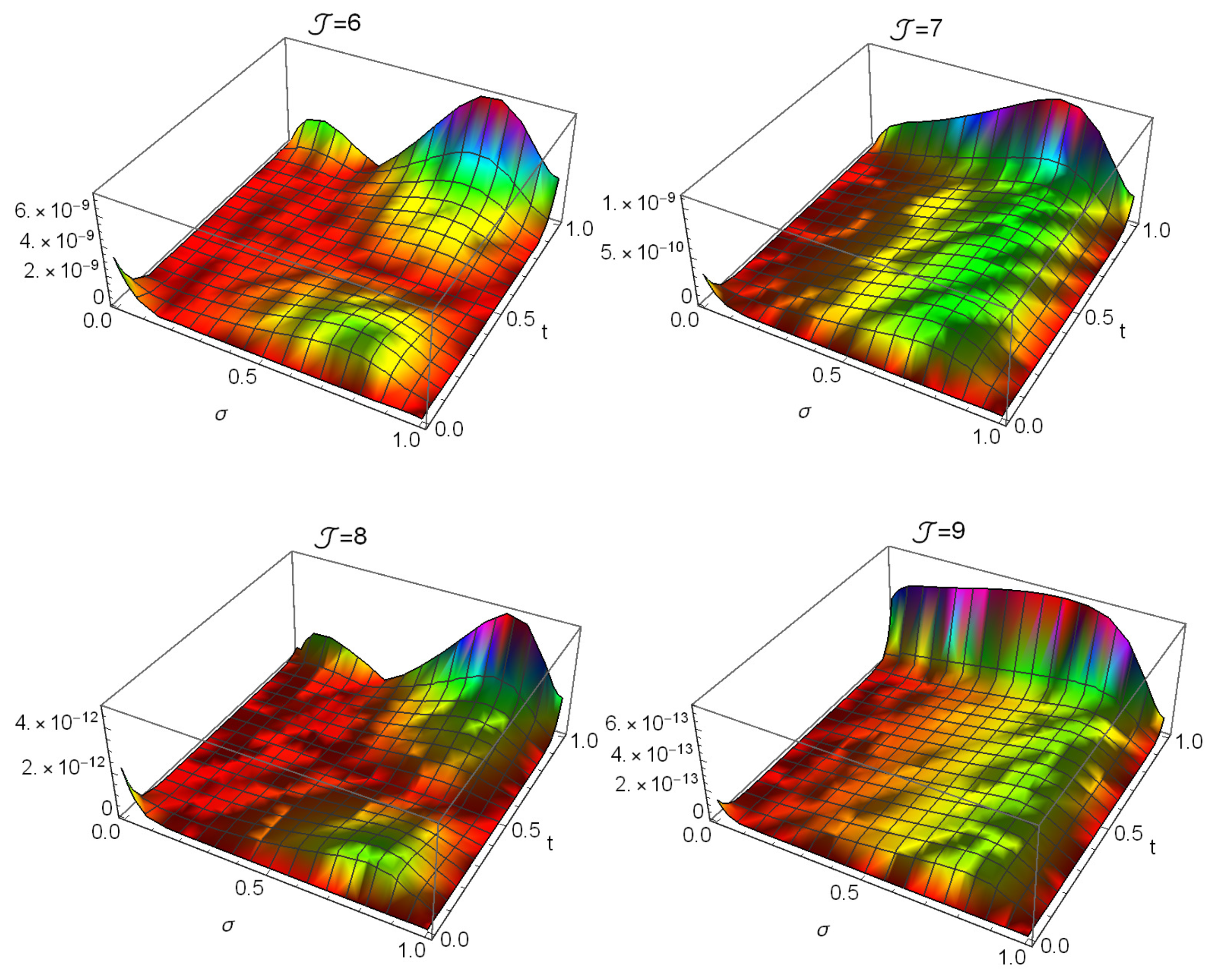
Table 1 presents a comparison of the absolute errors between our proposed technique at $\mathcal{J}=9$ and techniques presented in [48,49] when $t=0.0001$ and $ϵ=1$. Figure 1 illustrates the absolute errors at different values of $\mathcal{J}$ when $ϵ=1$. Table 2 shows the maximum absolute errors at different values of $\mathcal{J}$ and $ϵ=1$.

Table 1. The absolute errors of Example 1 at $t=0.0001$ and $ϵ=1$.

$\mathit{\sigma }$	Method in [48]	Method in [49]	Presented Technique at $\mathcal{J}=9$
0	$4.441\times {10}^{-16}$	$9.000\times {10}^{-9}$	$1.16351\times {10}^{-13}$
0.1	$3.908\times {10}^{-14}$	$1.111\times {10}^{-5}$	$1.77636\times {10}^{-15}$
0.2	$5.196\times {10}^{-14}$	$2.17\times {10}^{-5}$	$4.44089\times {10}^{-16}$
0.3	$9.104\times {10}^{-14}$	$3.314\times {10}^{-5}$	$1.33227\times {10}^{-15}$
0.4	$1.101\times {10}^{-13}$	$4.398\times {10}^{-5}$	$8.88178\times {10}^{-16}$
0.5	$1.492\times {10}^{-13}$	$5.465\times {10}^{-5}$	$8.88178\times {10}^{-16}$
0.6	$1.652\times {10}^{-13}$	$6.509\times {10}^{-5}$	0
0.7	$1.847\times {10}^{-13}$	$7.528\times {10}^{-5}$	0
0.8	$2.802\times {10}^{-13}$	$8.518\times {10}^{-5}$	$8.88178\times {10}^{-16}$
0.9	$2.385\times {10}^{-16}$	$9.474\times {10}^{-5}$	$8.88178\times {10}^{-16}$
1	$4.441\times {10}^{-16}$	$1.039\times {10}^{-4}$	0

Figure 1. The absolute errors of Example 1 at different values of $\mathcal{J}$.

Table 2. The maximum absolute errors of Example 1.

$\mathcal{J}$	3	4	5	6	7	8	9
Error	$3.1458\times {10}^{-4}$	$3.2918\times {10}^{-6}$	$4.3189\times {10}^{-7}$	$3.1246\times {10}^{-9}$	$3.6511\times {10}^{-10}$	$2.1285\times {10}^{-12}$	$1.7852\times {10}^{-13}$
CPU time	1.718	2.984	5.984	14.407	15.438	76.094	113.045

Example 2.

Consider the RHE [48,50].

$${\mathcal{Z}}_t+0.8{\mathcal{Z}}^3{\mathcal{Z}}_{\sigma }+2{\mathcal{Z}}^3{\mathcal{Z}}_{3\sigma }+18{\mathcal{Z}}^2{\mathcal{Z}}_{\sigma }{\mathcal{Z}}_{\sigma \sigma }+12\mathcal{Z}{\left({\mathcal{Z}}_{\sigma }\right)}^3=0.$$

(105)

with the following conditions:

$$\begin{array}{cc}\hfill & \mathcal{Z}(\sigma ,0)=2\sqrt[3]{ϵ{cos}^2\left(0.237171\sigma \right)},\hfill \\ & \mathcal{Z}(0,t)=2\sqrt[3]{ϵ{cos}^2\left(0.237171tϵ\right)},\hfill \\ & {\mathcal{Z}}_{\sigma }(0,t)=0.316228\sqrt[3]{ϵ{cos}^2\left(0.237171tϵ\right)}tan\left(0.237171tϵ\right),\hfill \\ & \mathcal{Z}(1,t)=2\sqrt[3]{ϵ{cos}^2(0.237171-0.237171tϵ)},\hfill \\ & {\mathcal{Z}}_{\sigma }(1,t)=-0.316228\sqrt[3]{ϵ{cos}^2(0.237171-0.237171tϵ)}tan(0.237171-0.237171tϵ),\hfill \end{array}$$

(106)

where the analytical solution is

$$\mathcal{Z}(\sigma ,t)=2\sqrt[3]{ϵ{cosh}^2\left({\displaystyle \frac{3}{8}}i\sqrt{0.4}(\sigma -tϵ)\right)}.$$

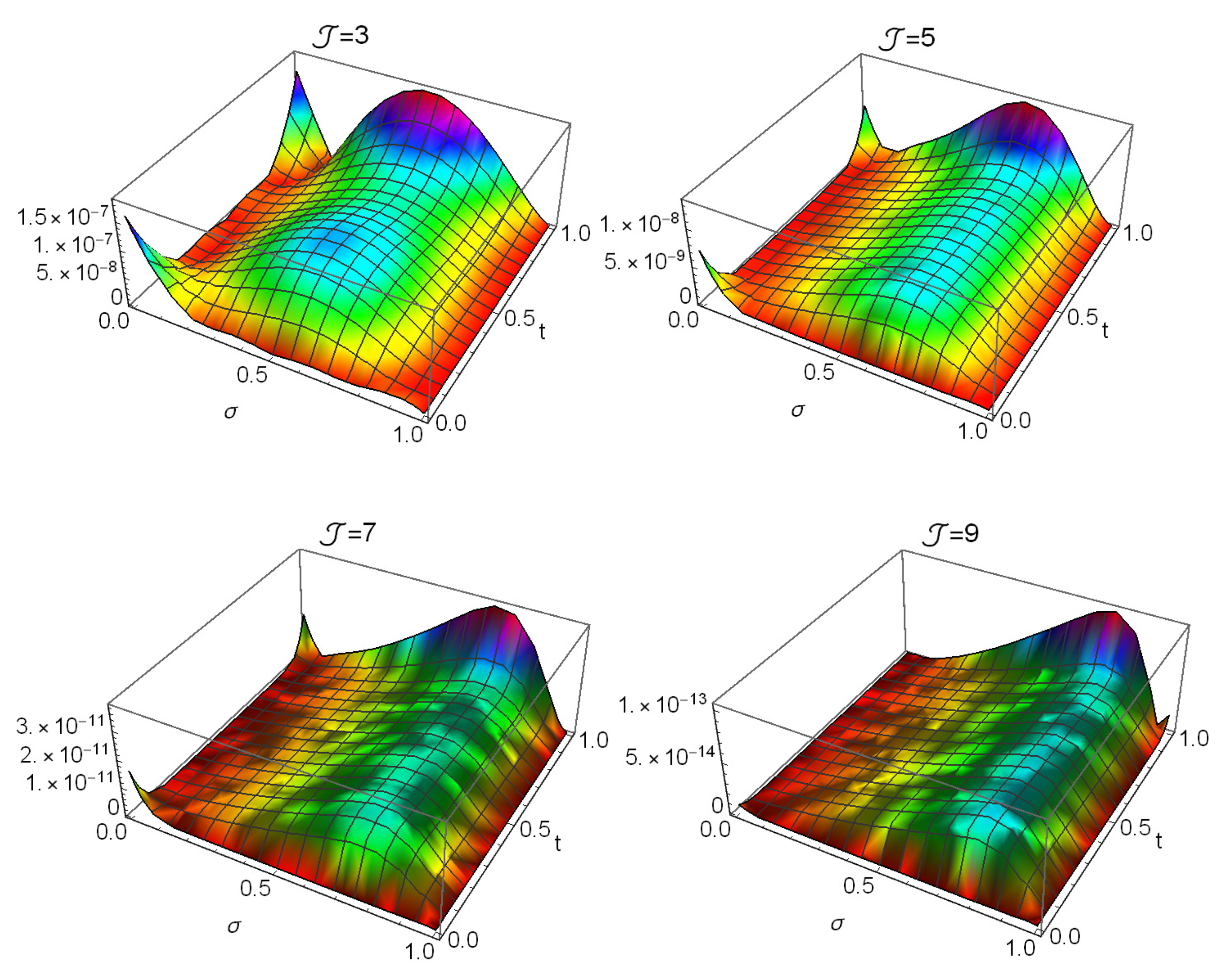
Table 3 presents a comparison of the absolute errors and relative absolute errors at $ϵ=0.1$ between our numerical technique at $\mathcal{J}=9$ and techniques presented in [48,50]. Figure 2 shows the absolute errors at different values of $\mathcal{J}$ and $ϵ=0.1$. Table 4 presents the CPU time used of Figure 2.

Table 3. The absolute errors of Example 2 at $ϵ=0.1$.

$(\mathit{\sigma },\mathit{t})$	Absolute Error			Relative Error
	Method in [48]	Method in [50]	Presented Method	Method in [48]	Method in [50]	Presented Method
(0, 0)	$1.11\times {10}^{-16}$	$2.31\times {10}^{-11}$	$6.43929\times {10}^{-15}$	$1.20\times {10}^{-16}$	$2.48\times {10}^{-11}$	$6.93652\times {10}^{-15}$
(0, 0.2)	$5.55\times {10}^{-16}$	$2.57\times {10}^{-10}$	$2.22045\times {10}^{-16}$	$5.98\times {10}^{-16}$	$2.76\times {10}^{-10}$	$2.39192\times {10}^{-16}$
(0, 0.4)	$1.11\times {10}^{-16}$	$4.90\times {10}^{-10}$	0	$1.20\times {10}^{-16}$	$5.28\times {10}^{-10}$	0
(0, 0.6)	$7.77\times {10}^{-16}$	$6.52\times {10}^{-10}$	0	$8.37\times {10}^{-16}$	$7.03\times {10}^{-10}$	0
(0, 0.8)	$3.33\times {10}^{-16}$	$7.62\times {10}^{-10}$	0	$3.59\times {10}^{-16}$	$8.21\times {10}^{-10}$	0
(0, 1)	$8.88\times {10}^{-16}$	$9.99\times {10}^{-10}$	$9.99201\times {10}^{-16}$	$9.57\times {10}^{-16}$	$1.08\times {10}^{-15}$	$1.07656\times {10}^{-15}$
(0.5, 0)	$1.11\times {10}^{-16}$	$7.10\times {10}^{-11}$	$1.11022\times {10}^{-16}$	$1.20\times {10}^{-16}$	$7.69\times {10}^{-11}$	$1.11022\times {10}^{-16}$
(0.5, 0.2)	$1.52\times {10}^{-10}$	$5.30\times {10}^{-9}$	$2.78666\times {10}^{-14}$	$1.64\times {10}^{-10}$	$5.73\times {10}^{-9}$	$2.78666\times {10}^{-14}$
(0.5, 0.4)	$1.81\times {10}^{-10}$	$9.63\times {10}^{-9}$	$2.76446\times {10}^{-14}$	$1.95\times {10}^{-10}$	$1.04\times {10}^{-8}$	$2.76446\times {10}^{-14}$
(0.5, 0.6)	$6.65\times {10}^{-11}$	$1.35\times {10}^{-8}$	$2.69784\times {10}^{-14}$	$7.19\times {10}^{-11}$	$1.45\times {10}^{-8}$	$2.69784\times {10}^{-14}$
(0.5, 0.8)	$2.34\times {10}^{-10}$	$1.68\times {10}^{-8}$	$2.68674\times {10}^{-14}$	$2.53\times {10}^{-10}$	$1.82\times {10}^{-8}$	$2.68674\times {10}^{-14}$
(0.5, 1)	$2.49\times {10}^{-10}$	$4.39\times {10}^{-8}$	$5.89528\times {10}^{-14}$	$2.69\times {10}^{-10}$	$4.74\times {10}^{-8}$	$5.89528\times {10}^{-14}$
(1, 0)	$2.22\times {10}^{-16}$	$9.99\times {10}^{-16}$	$3.33067\times {10}^{-16}$	$2.44\times {10}^{-16}$	$1.10\times {10}^{-15}$	$3.33067\times {10}^{-16}$
(1, 0.2)	$2.22\times {10}^{-16}$	0	0	$2.44\times {10}^{-16}$	0	0
(1, 0.4)	$5.55\times {10}^{-16}$	$9.99\times {10}^{-16}$	$1.11022\times {10}^{-16}$	$6.08\times {10}^{-16}$	$1.10\times {10}^{-15}$	$1.11022\times {10}^{-16}$
(1, 0.6)	0	$1.11\times {10}^{-15}$	$1.11022\times {10}^{-16}$	0	$1.22\times {10}^{-15}$	$1.11022\times {10}^{-16}$
(1, 0.8)	$1.11\times {10}^{-16}$	$1.11\times {10}^{-15}$	0	$1.22\times {10}^{-16}$	$1.22\times {10}^{-15}$	0
(1, 1)	$1.11\times {10}^{-16}$	0	$1.65423\times {10}^{-14}$	$1.21\times {10}^{-16}$	0	$1.65423\times {10}^{-14}$

Figure 2. The absolute errors of Example 2 at different values of $\mathcal{J}$.

Table 4. CPU time of Figure 2.

$\mathcal{J}$	3	5	7	9
Cpu time	2.032	7.782	27.39	189.532

Example 3.

Consider the FWE

$${\mathcal{Z}}_t-{\mathcal{Z}}_{\sigma \sigma t}+{\mathcal{Z}}_{\sigma }-\mathcal{Z}{\mathcal{Z}}_{3\sigma }+\mathcal{Z}{\mathcal{Z}}_{\sigma }-3{\mathcal{Z}}_{\sigma }{\mathcal{Z}}_{\sigma \sigma }=0,$$

(107)

with the following conditions:

$$\begin{array}{cc}\hfill \mathcal{Z}(\sigma ,0)& ={\displaystyle \frac{4e^{\sigma /2}}{3}},\hfill \\ \hfill \mathcal{Z}(0,t)& ={\displaystyle \frac{4}{3}}{e}^{-{\displaystyle \frac{2t}{3}}},{\mathcal{Z}}_{\sigma }(0,t)={\displaystyle \frac{2}{3}}{e}^{-{\displaystyle \frac{2t}{3}}},\hfill \\ \hfill \mathcal{Z}(1,t)& ={\displaystyle \frac{4}{3}}{e}^{{\displaystyle \frac{1}{2}}-{\displaystyle \frac{2t}{3}}},{\mathcal{Z}}_{\sigma }(1,t)={\displaystyle \frac{2}{3}}{e}^{{\displaystyle \frac{1}{2}}-{\displaystyle \frac{2t}{3}}},\hfill \end{array}$$

(108)

where the analytical solution is

$$\mathcal{Z}(\sigma ,t)={\displaystyle \frac{4}{3}}{e}^{{\displaystyle \frac{\sigma }{2}}-{\displaystyle \frac{2t}{3}}}.$$

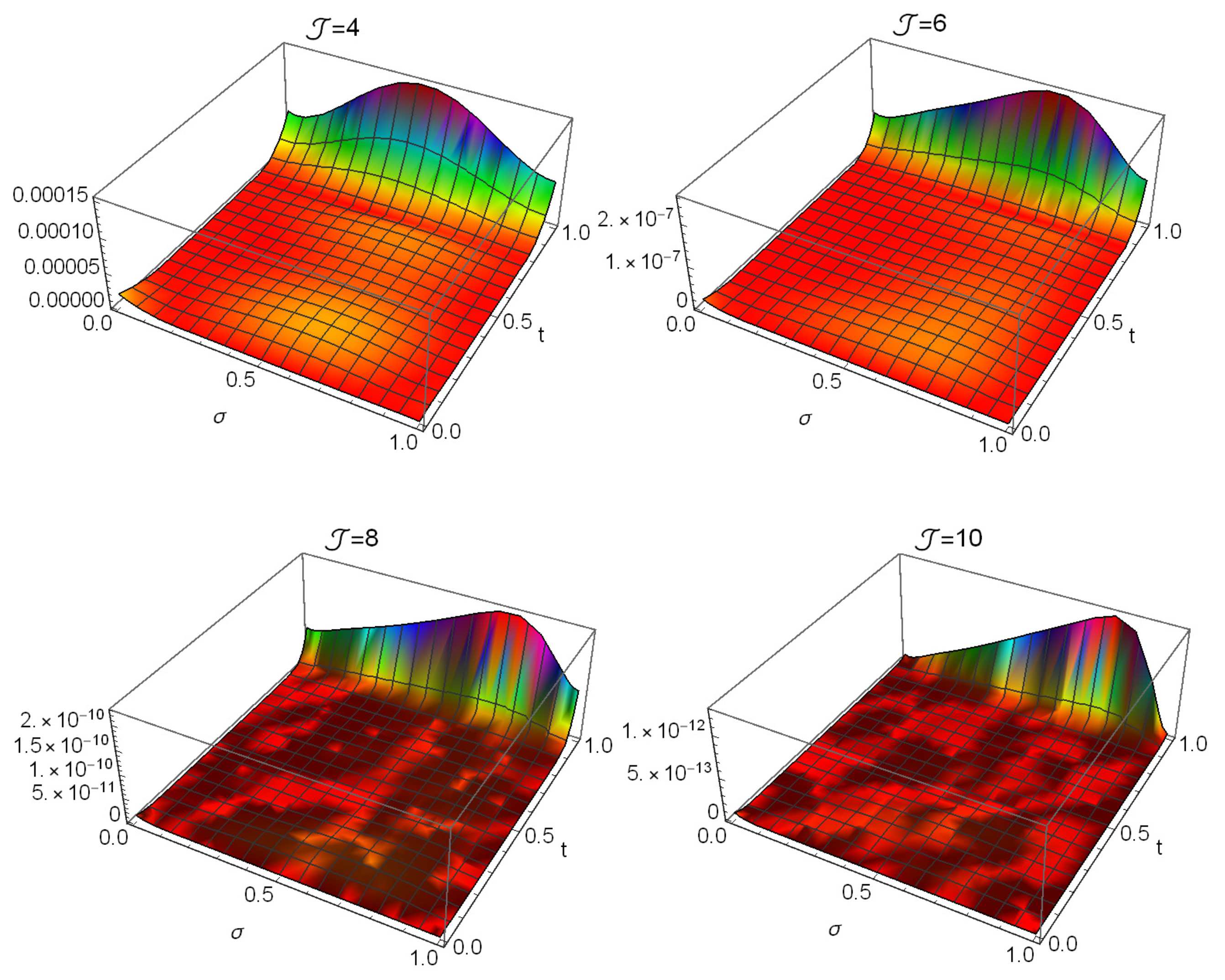
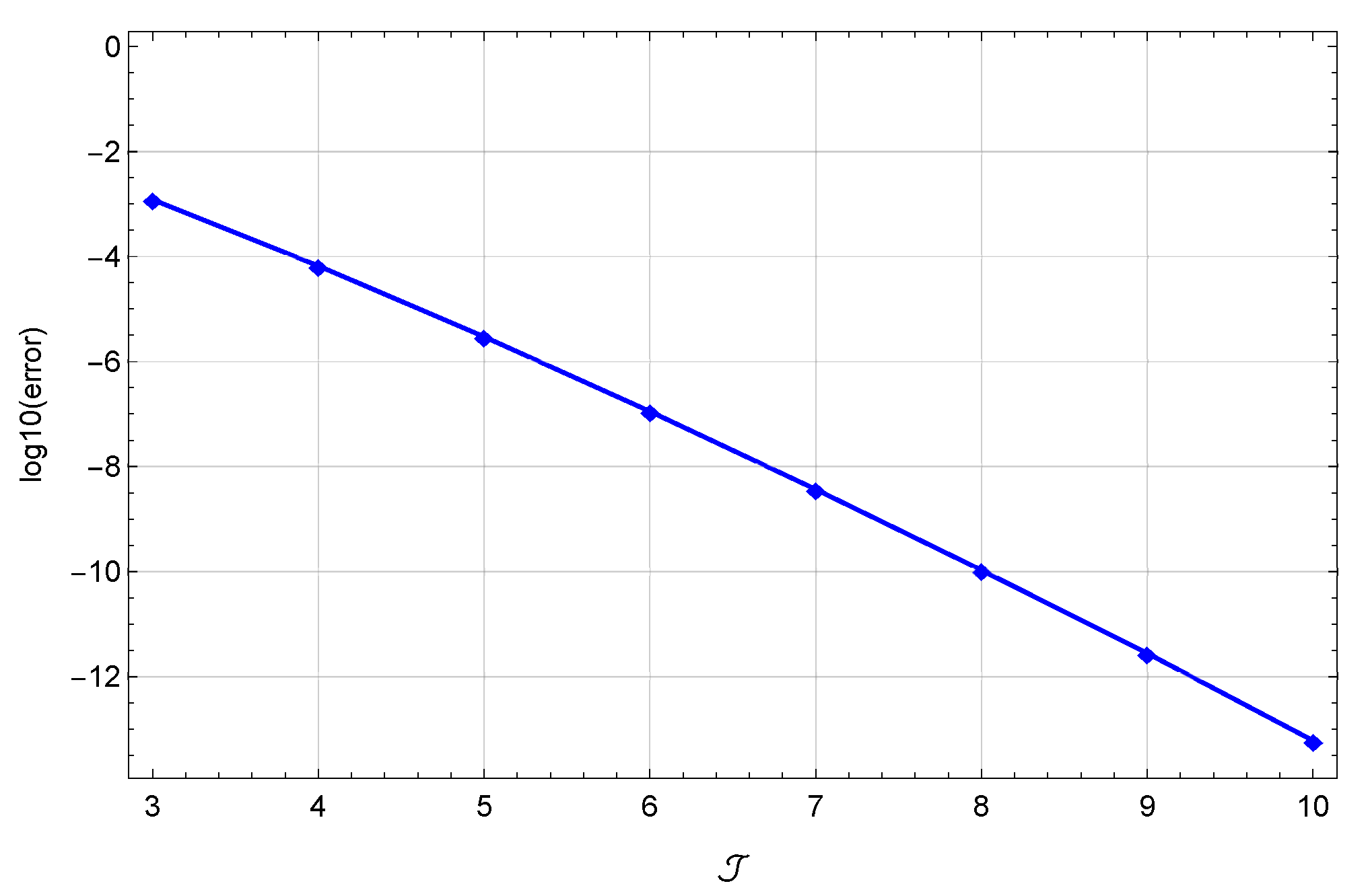
Table 5 shows the absolute and relative errors when $\mathcal{J}=10$ at different values of σ and t. Figure 3 shows the absolute errors at different values of $\mathcal{J}$. Finally, Figure 4 illustrates the Log10 of maximum absolute errors at different values of $\mathcal{J}$.

Table 5. The absolute errors of Example 3 at $\mathcal{J}=10$.

$(\mathit{\sigma },\mathit{t})$	Absolute Error	Relative Error	CPU Time
(0, 0)	$5.9508\times {10}^{-14}$	$4.4631\times {10}^{-14}$	295.545
(0.1, 0.1)	$6.43929\times {10}^{-15}$	$4.91064\times {10}^{-15}$
(0.2, 0.2)	$8.43769\times {10}^{-15}$	$6.54277\times {10}^{-15}$
(0.3, 0.3)	$5.10703\times {10}^{-15}$	$4.02665\times {10}^{-15}$
(0.4, 0.4)	$8.43769\times {10}^{-15}$	$6.76454\times {10}^{-15}$
(0.5, 0.5)	$1.55431\times {10}^{-14}$	$1.26704\times {10}^{-14}$
(0.6, 0.6)	$6.43929\times {10}^{-15}$	$5.33739\times {10}^{-15}$
(0.7, 0.7)	$1.33227\times {10}^{-15}$	$1.12285\times {10}^{-15}$
(0.8, 0.8)	$4.21885\times {10}^{-15}$	$3.61544\times {10}^{-15}$
(0.9, 0.9)	$1.79856\times {10}^{-14}$	$1.56722\times {10}^{-14}$
(1, 1)	$4.19664\times {10}^{-14}$	$3.71831\times {10}^{-14}$

Figure 3. The absolute errors of Example 3 at different values of $\mathcal{J}$.

Figure 4. The Log10(errors) of Example 3.

8. Concluding Remarks

In this study, a new strategy based on the typical collocation method was applied to the third-order Gilson–Pickering equation and its notable special cases. The shifted Pell polynomials were introduced as basis functions. New operational formulas for the shifted Pell polynomials were stated and proved. These were the fundamental bases to design the proposed numerical algorithms. In addition, an upper bound for these polynomials was developed and used in the convergence examination for the double-shifted Pell expansion. The numerical examples demonstrated the algorithms’ reliability and effectiveness. In addition, compared with some existing schemes, the shifted-Pell collocation approach yielded significantly smaller absolute and relative errors and achieved excellent accuracy even for small polynomial degrees. As future work, we aim to extend the shifted-Pell collocation framework to handle other important problems, such as fractional-order and integro-differential equations, as well as nonlinear partial differential equations in higher dimensions. In addition, from a theoretical perspective, we aim to generalize the basis functions used and apply them to several applications. All codes were written and debugged using Mathematica 11 on an HP Z420 Workstation, with an Intel(R) Xeon(R) CPU E5-1620 processor, v2, 3.70 GHz; 16 GB of RAM, DDR3; and 512 GB of storage.

References

- Campos, L.M.B.C. Non-Linear Differential Equations and Dynamical Systems, 1st ed.; CRC Press, Taylor & Francis: Boca Raton, FL, USA, 2019; p. 305. [Google Scholar]
- Veiga, H.B.; Minhos, F.; Van Goethem, N.; Rodrigues, L.S. (Eds.) Nonlinear Differential Equations and Applications; CIM Series in Mathematical Sciences; Springer: Cham, Switzerland, 2024; Volume 7. [Google Scholar]
- Alalyani, A.; Ahmed, D.M.; Mahmood, B.A. An Efficient Numerical Technique for Solving the Korteweg–de Vries–Burgers Equation. Int. J. Anal. Appl. 2025, 23, 22. [Google Scholar] [CrossRef] [Scilit]
- Abd-Elhameed, W.M.; Alqubori, O.M.; Atta, A.G. A collocation approach for the nonlinear fifth-order KdV equations using certain shifted Horadam polynomials. Mathematics 2025, 13, 300. [Google Scholar] [CrossRef] [Scilit]
- Rufai, M.A.; Kosti, A.A.; Anastassi, Z.A.; Carpentieri, B. A New Two-Step Hybrid Block Method for the FitzHugh–Nagumo Model Equation. Mathematics 2023, 12, 51. [Google Scholar] [CrossRef] [Scilit]
- Choudhary, R.; Singh, S.; Das, P.; Kumar, D. A higher order stable numerical approximation for time-fractional non-linear Kuramoto–Sivashinsky equation based on quintic B-spline. Math. Methods Appl. Sci. 2024, 47, 11953–11975. [Google Scholar] [CrossRef] [Scilit]
- Aychluh, M.; Ayalew, M. The fractional power series method for solving the nonlinear Kuramoto–Sivashinsky equation. Int. J. Appl. Comput. Math. 2025, 11, 29. [Google Scholar] [CrossRef] [Scilit]
- Ben-Romdhane, M.; Temimi, H. An Iterative Finite Difference Method for Solving Nonlinear Gordon-Type Problems. Mathematics 2025, 13, 2084. [Google Scholar] [CrossRef] [Scilit]
- Ahmed, H.M.; Izadi, M. An accurate approximation technique based on Schröder operational matrices for numerical treatments of time-fractional nonlinear generalized Kawahara equation. Bound. Value Probl. 2025, 2025, 90. [Google Scholar] [CrossRef] [Scilit]
- Ahmed, H.M.; Hafez, R.M.; Abd-Elhameed, W.M. A computational strategy for nonlinear time-fractional generalized Kawahara equation using new eighth-kind Chebyshev operational matrices. Phys. Scr. 2024, 99, 045250. [Google Scholar] [CrossRef] [Scilit]
- Barletti, L.; Brugnano, L.; Gurioli, G.; Iavernaro, F. Recent advances in the numerical solution of the Nonlinear Schrödinger Equation. J. Comput. Appl. Math. 2024, 445, 115826. [Google Scholar] [CrossRef] [Scilit]
- Köcher, N.; Rose, H.; Bharadwaj, S.S.; Schumacher, J.; Schumacher, S. Numerical solution of nonlinear Schrödinger equation by a hybrid pseudospectral-variational quantum algorithm. Sci. Rep. 2025, 15, 23478. [Google Scholar] [CrossRef] [Scilit]
- Shen, J.; Tang, T.; Wang, L.L. Spectral Methods: Algorithms, Analysis and Applications; Springer: Berlin/Heidelberg, Germany, 2011; Volume 41. [Google Scholar]
- Nikiforov, F.; Uvarov, V.B. Special Functions of Mathematical Physics; Springer: Berlin/Heidelberg, Germany, 1988; Volume 205. [Google Scholar]
- Hafez, R.M.; Abd-Elhameed, W.M.; Ahmed, H.M.; Abdelkawy, M.A.; Sabir, Z. An innovative shifted generalized Chebyshev collocation scheme for pantograph-type delay equations. Alex. Eng. J. 2025, 132, 110–132. [Google Scholar] [CrossRef] [Scilit]
- Tural-Polat, S.N.; Dincel, A.T. Numerical solution method for multi-term variable order fractional differential equations by shifted Chebyshev polynomials of the third kind. Alex. Eng. J. 2022, 61, 5145–5153. [Google Scholar] [CrossRef] [Scilit]
- Abdelhakem, M.; Alaa-Eldeen, T.; Baleanu, D.; Alshehri, M.G.; El-Kady, M. Approximating real-life BVPs via Chebyshev polynomials’ first derivative pseudo-Galerkin method. Fractal Fract. 2021, 5, 165. [Google Scholar] [CrossRef] [Scilit]
- Ganji, R.M.; Jafari, H.; Kgarose, M.; Mohammadi, A. Numerical solutions of time-fractional Klein–Gordon equations by clique polynomials. Alex. Eng. J. 2021, 60, 4563–4571. [Google Scholar] [CrossRef] [Scilit]
- Abd-Elhameed, W.M.; Al-Mehmadi, A.H.; Alsafri, N.M.A.; Alqubori, O.M.; Adel, M.; Atta, A.G. Spectral collocation approach for solving the time-fractional Kuramoto–Sivashinsky equation using the Fibonacci coefficient polynomials. AIMS Math. 2023, 10, 18070–18093. [Google Scholar] [CrossRef] [Scilit]
- Saad, K.M.; Srivastava, R. Non-standard finite difference and Vieta–Lucas orthogonal polynomials for the multi-space fractional-order coupled Korteweg–de Vries equation. Symmetry 2024, 16, 242. [Google Scholar] [CrossRef] [Scilit]
- Abd-Elhameed, W.M.; Abdelkawy, M.A.; Alqubori, O.M.; Atta, A.G. Pell coefficient polynomials for solving linear hyperbolic first-order partial differential equations via the Tau approach. Electron. Res. Arch. 2025, 33, 6012–6035. [Google Scholar] [CrossRef] [Scilit]
- Avazzadeh, Z.; Hassani, H.; Ebadi, M.J.; Eshkaftaki, A.B. A new approach of generalized shifted Vieta–Fibonacci polynomials to solve nonlinear variable order time-fractional Burgers–Huxley equations. Phys. Scr. 2024, 99, 125258. [Google Scholar] [CrossRef] [Scilit]
- Abd-Elhameed, W.M.; Alsulami, S.A.; Alqubori, O.M.; Alsafri, N.M.A.; Adel, M.; Atta, A.G. Spectral solutions for nonlinear static beam and fractional Riccati problems using new Lucas coefficient polynomials. AIMS Math. 2023, 10, 20862–20890. [Google Scholar] [CrossRef] [Scilit]
- Ali, I.; Haq, S.; Nisar, K.S.; Baleanu, D. An efficient numerical scheme based on Lucas polynomials for the study of multidimensional Burgers-type equations. Adv. Differ. Equ. 2021, 2021, 43. [Google Scholar] [CrossRef] [Scilit]
- Çayan, S.; Sezer, M.; Çevik, M. Pell matrix collocation method for solving damped wave equation. In Proceedings of the 3rd International Students Science Congress, İzmir, Turkey, 3–4 May 2019; pp. 281–289. [Google Scholar]
- Singh, P.K.; Ray, S.S. A numerical approach based on Pell polynomial for solving stochastic fractional differential equations. Numer. Algorithms 2024, 97, 1513–1534. [Google Scholar] [CrossRef] [Scilit]
- Yaslan, H.Ç. Pell polynomial solution of the nonlinear variable order space fractional PDEs. J. Fract. Calc. Appl. 2025, 16, 1–16. [Google Scholar] [CrossRef] [Scilit]
- Çerdik Yaslan, H. Pell polynomial solution of the fractional differential equations in the Caputo–Fabrizio sense. Indian J. Pure Appl. Math. 2024, 1–12. [Google Scholar] [CrossRef] [Scilit]
- Shiri, N.; Ordokhani, Y.; Sabermahani, S. Fractional-order Pell hybrid functions for solving variable-order fractional differential equations and their application in chemistry. Iran. J. Math. Chem. 2025, 16, 223–244. [Google Scholar]
- Canuto, C.; Hussaini, M.Y.; Quarteroni, A.; Zang, T.A. Spectral Methods: Fundamentals in Single Domains; Scientific Computation; Springer: Berlin/Heidelberg, Germany, 2006. [Google Scholar]
- Boyd, J.P. Chebyshev and Fourier Spectral Methods, 2nd ed.; Dover Publications: Garden City, NY, USA, 2001. [Google Scholar]
- Yang, X.; Zhang, Z. Superconvergence analysis of a robust orthogonal Gauss collocation method for 2D fourth-order subdiffusion equations. J. Sci. Comput. 2024, 100, 62. [Google Scholar] [CrossRef] [Scilit]
- Bartwal, P.; Pandey, A.K.; Upreti, H. Impact of anisotropic slip on magnetized tangent hyperbolic fluid flow over a rotating disk: A Legendre wavelet collocation method. Int. Commun. Heat Mass Transf. 2024, 159, 108081. [Google Scholar] [CrossRef] [Scilit]
- Ahmed, H.M. A new first finite class of classical orthogonal polynomials operational matrices: An application for solving fractional differential equations. Contemp. Math. 2023, 4, 974–979. [Google Scholar] [CrossRef] [Scilit]
- Atta, A.G.; Abdelkawy, M.A.; Napoli, A.; Abd-Elhameed, W.M. Galerkin approach by certain shifted Jacobi polynomials for solving the time-fractional Black–Scholes equation. Bound. Value Probl. 2025, 2025, 138. [Google Scholar] [CrossRef] [Scilit]
- Alsuyuti, M.M.; Doha, E.H.; Ezz-Eldien, S.S. Numerical simulation for classes of one- and two-dimensional multi-term time-fractional diffusion and diffusion-wave equations based on shifted Jacobi Galerkin scheme. Math. Methods Appl. Sci. 2025, 48, 8217–8244. [Google Scholar] [CrossRef] [Scilit]
- Abd-Elhameed, W.M.; Machado, J.A.T.; Youssri, Y.H. Hypergeometric fractional derivatives formula of shifted Chebyshev polynomials: Tau algorithm for a type of fractional delay differential equations. Int. J. Nonlinear Sci. Numer. Simul. 2022, 23, 1253–1268. [Google Scholar] [CrossRef] [Scilit]
- El-Sayed, A.A.E.; Boulaaras, S.; Sweilam, N.H. Numerical solution of the fractional-order logistic equation via the first-kind Dickson polynomials and spectral tau method. Math. Methods Appl. Sci. 2023, 46, 8004–8017. [Google Scholar] [CrossRef] [Scilit]
- Abdelhakem, M.; Abdelhamied, D.; El-Kady, M.; Youssri, Y.H. Two modified shifted Chebyshev–Galerkin operational matrix methods for even-order partial boundary value problems. Bound. Value Probl. 2025, 2025, 34. [Google Scholar] [CrossRef] [Scilit]
- Ji, T.; Hou, J.; Yang, C. The operational matrix of Chebyshev polynomials for solving pantograph-type Volterra integro-differential equations. Adv. Contin. Discret. Model. 2022, 2022, 57. [Google Scholar] [CrossRef] [Scilit]
- Abd-Elhameed, W.M. On solving linear and nonlinear sixth-order two-point boundary value problems via an elegant harmonic numbers operational matrix of derivatives. CMES Comput. Model. Eng. Sci. 2014, 101, 159. [Google Scholar]
- Isah, A.; Phang, C. Operational matrix based on Genocchi polynomials for solution of delay differential equations. Ain Shams Eng. J. 2018, 9, 2123–2128. [Google Scholar] [CrossRef] [Scilit]
- Yousefi, S.A.; Behroozifar, M.; Dehghan, M. Numerical solution of the nonlinear age-structured population models by using the operational matrices of Bernstein polynomials. Appl. Math. Model. 2012, 36, 945–963. [Google Scholar] [CrossRef] [Scilit]
- Kumar, S.; Gupta, V.; Zeidan, D. An efficient collocation technique based on operational matrix of fractional-order Lagrange polynomials for solving the space-time fractional-order partial differential equations. Appl. Numer. Math. 2024, 204, 249–264. [Google Scholar] [CrossRef] [Scilit]
- Öztürk, Y.; Gülsu, M. An operational matrix method for solving Lane–Emden equations arising in astrophysics. Math. Methods Appl. Sci. 2014, 37, 2227–2235. [Google Scholar] [CrossRef] [Scilit]
- Andrews, G.; Askey, R.; Roy, R. Special Functions; Cambridge University Press: Cambridge, UK, 1999. [Google Scholar]
- Gilson, C.; Pickering, A. Factorization and Painlevé analysis of a class of nonlinear third-order partial differential equations. J. Phys. A Math. Gen. 1995, 28, 2871. [Google Scholar] [CrossRef] [Scilit]
- Akbar, T.; Haq, S.; Arifeen, S.U.; Iqbal, A. Numerical Solution of Third-Order Rosenau–Hyman and Fornberg–Whitham Equations via B-Spline Interpolation Approach. Axioms 2024, 13, 501. [Google Scholar] [CrossRef] [Scilit]
- Arslan, D. The comparison study of hybrid method with RDTM for solving Rosenau–Hyman equation. Appl. Math. Nonlinear Sci. 2020, 5, 267–274. [Google Scholar] [CrossRef] [Scilit]
- Cinar, M.; Secer, A.; Bayram, M. An application of Genocchi wavelets for solving the fractional Rosenau–Hyman equation. Alex. Eng. J. 2021, 60, 5331–5340. [Google Scholar] [CrossRef] [Scilit]
Disclaimer/Publisher’s Note: The statements, opinions and data contained in all publications are solely those of the individual author(s) and contributor(s) and not of MDPI and/or the editor(s). MDPI and/or the editor(s) disclaim responsibility for any injury to people or property resulting from any ideas, methods, instructions or products referred to in the content. |
© 2026 by the authors. Licensee MDPI, Basel, Switzerland. This article is an open access article distributed under the terms and conditions of the Creative Commons Attribution (CC BY) license.