An Improved Particle Swarm Optimization for Three-Dimensional Indoor Positioning with Ultra-Wideband Communications for LOS/NLOS Channels ^†

Abstract

In this study, an improved particle swarm optimization (PSO) algorithm is designed to construct a weighting model for line-of-sight (LOS) and non-line-of-sight (NLOS) channels in an ultra-wideband (UWB) indoor positioning system. In the proposed algorithm, the particle position represents candidate weight vectors, and the fitness function is defined by the 3D positioning error over multiple test points. An optimized weight modeling framework is proposed for a multi-anchor, three-dimensional UWB indoor positioning system under LOS and NLOS channels. First, the three-dimensional positioning problem is formulated as a multilateration model, and the tag coordinates are estimated via a linearized matrix equation solved by the least-squares method, which explicitly links anchor geometry and ranging errors to the positioning accuracy. To evaluate the proposed method, extensive ranging and positioning experiments are conducted in a realistic indoor environment using up to eight anchors with different LOS/NLOS configurations, including dynamic scenarios with varying numbers of NLOS anchors. The results show that, compared with the conventional unweighted multi-anchor scheme, the PSO-based weighting model can reduce the average 3D positioning error by more than 30% in typical LOS-dominant settings and significantly suppress error bursts in severe NLOS conditions. These findings demonstrate that the combination of mathematical modeling, least-squares estimation, and swarm intelligence optimization provides an effective tool for designing intelligent engineering positioning systems in complex indoor environments, which aligns with the development of smart factories and industrial Internet-of-Things (IIoT) applications.

1. Introduction

With the continuous advancement of urbanization, the demand for accurate indoor positioning technologies has increased significantly. Studies have reported that individuals spend the majority of their daily lives within indoor environments, accounting for approximately 70% to 90% of their total time [1]. Consequently, positioning systems have evolved into a fundamental enabling technology that supports a wide range of modern applications. Based on their operating environments, positioning technologies are generally categorized into outdoor and indoor systems. Outdoor positioning is predominantly supported by Global Navigation Satellite Systems (GNSS), such as the Global Positioning System (GPS) and China’s BeiDou Navigation Satellite System, which are extensively utilized in both military and civilian applications. Under open-sky conditions, these systems typically achieve positioning accuracies in the order of 5–10 m [2,3]. However, in indoor environments, satellite signals suffer from severe attenuation, diffraction, and multipath propagation caused by walls, floors, ceilings, and other obstacles, rendering GNSS-based positioning unreliable or ineffective [4]. As a result, conventional outdoor positioning technologies cannot be directly extended to indoor scenarios, necessitating the development of dedicated indoor positioning solutions.

In recent years, the rapid proliferation of smartphones, wearable devices, and smart terminals has led to a dramatic increase in wireless data traffic, thereby imposing stringent requirements on transmission rate, latency, and system reliability. To meet these demands, advanced wireless communication technologies such as fifth-generation mobile communication (5G) and LTE-Advanced (LTE-A) have been introduced, offering enhanced spectral efficiency, higher throughput, and reduced latency [5]. These characteristics make 5G a key enabler for emerging paradigms such as the Internet of Things (IoT) and the Artificial Intelligence of Things (AIoT). The 5G framework integrates multiple innovative technologies, including massive multiple-input–multiple-output (MIMO), ultra-dense network deployment, novel multiple-access schemes, full-spectrum utilization, and software-defined networking (SDN)-based architectures, enabling high-capacity, high-reliability, and low-latency communication services [6]. Beyond communications, these technological advancements also provide new opportunities for wireless positioning. In particular, positioning techniques exploiting millimeter-wave (mmWave) frequencies in 5G systems have attracted considerable attention, as their propagation characteristics are comparable to those of ultra-wideband (UWB) systems.

A wide variety of technologies have been investigated for indoor positioning, including LiDAR [7], Wi-Fi [8], ZigBee [9], Bluetooth [10], radio frequency identification (RFID) [11,12], infrared-based systems, and ultra-wideband (UWB) technology [13,14,15]. Among these approaches, UWB has emerged as a particularly promising solution due to its fine time resolution and strong resistance to multipath interference, enabling centimeter-level positioning accuracy [16]. Such high precision is essential in indoor environments, where even small localization errors may lead to incorrect spatial interpretation or misidentification of room-level positions [17]. Owing to these advantages, UWB is widely regarded as one of the most effective technologies for high-accuracy indoor positioning applications.

As indoor environments become increasingly complex, future positioning systems are expected to evolve from two-dimensional to three-dimensional localization. In scenarios such as multi-story buildings, warehouses, and industrial facilities, planar positioning alone is insufficient to represent actual spatial relationships. Three-dimensional positioning provides a more comprehensive description of objects or human locations by incorporating vertical information, which is particularly important in environments with significant height variations [18]. In this study, UWB technology is employed for indoor localization, and a three-dimensional positioning model is established to estimate spatial coordinates. Experimental results demonstrate that when all anchors and tags operate under line-of-sight (LOS) conditions, positioning errors can be constrained to the centimeter level. However, the presence of even a single anchor under non-line-of-sight (NLOS) conditions can cause a substantial degradation in positioning accuracy. Further experiments using multiple anchors indicate that optimal positioning performance is achieved only when all anchors maintain LOS links.

In practical indoor deployments, it is often unavoidable that some anchors operate under NLOS conditions. Taking into account the requirements of UWB positioning systems, including real-time performance, continuity, robustness to noise, and computational efficiency, particle swarm optimization (PSO) is selected as a suitable and balanced optimization approach [19,20,21,22]. Accordingly, this study adopts PSO instead of alternative metaheuristic algorithms such as the genetic algorithm (GA) [23], firefly algorithm (FA), or social spider optimization (SSO). To mitigate the adverse effects of NLOS conditions on localization accuracy, an improved PSO-based method is proposed to suppress the influence of NLOS measurements. By adaptively adjusting the weightings of multi-anchor ranging information within the PSO framework, the proposed approach effectively reduces NLOS-induced errors in three-dimensional positioning. The results indicate that the proposed method enhances system robustness and improves localization feasibility across diverse and challenging indoor environments.

2. Positioning Methods

2.1. Ultra-Wideband

In specific applications, UWB technology commonly utilizes a frequency range from 3.1 GHz to 10.6 GHz. This broad frequency range provides ample space to transmit large amounts of data and allows signals to convey more information in a shorter period of time. Moreover, a characteristic of UWB signals is their very low transmission power, which helps to minimize interference with other wireless communication devices while maintaining high communication quality and achieving precise time positioning and distance measurement. These features make UWB highly useful in applications requiring high data transmission rates and high precision in positioning, such as indoor positioning systems, IoT devices, and short-range wireless communications [24].

2.1.1. Ultra-Wideband Standards

UWB technology is regulated by a series of international and national standards, which guide its development, application, and management. Among these, the IEEE 802.15.4a/z standard [25], established by the IEEE, focuses on precise positioning and timing for low-power personal area networks, applicable to indoor navigation, asset tracking, and IoT devices. In the United States, the Federal Communications Commission regulates the frequency band usage and transmission power of UWB, limiting it to the 3.1 to 10.6 GHz range to minimize interference with other wireless services [25]. In Europe, standards set by the European Telecommunications Standards Institute define technical requirements and testing methods to ensure the compatibility and performance of UWB devices. Additionally, the International Organization for Standardization and the International Electrotechnical Commission have also established international standards involving UWB technology, aimed at providing a unified global technical framework to promote its international recognition and widespread application. As technology continues to advance, these standards will continually be updated to address new technical challenges and market demands.

2.1.2. DW1000 Chip

DW1000 is a UWB wireless chip developed by Decawave, widely used in indoor positioning and communication systems that require high precision and low power consumption. This chip is based on the IEEE 802.15.4-2011 UWB standard [25] and is specially designed to provide accurate time measurement capabilities, supporting cm-level positioning accuracy. A distinctive feature of the DW1000 chip is its ability to operate across different UWB frequency bands, including the 3.5 GHz to 6.5 GHz range, and it can achieve data transfer rates of up to 10 Mbps upon adjusting the pulse repetition frequency [26,27].

2.1.3. ESP32 UWB Module

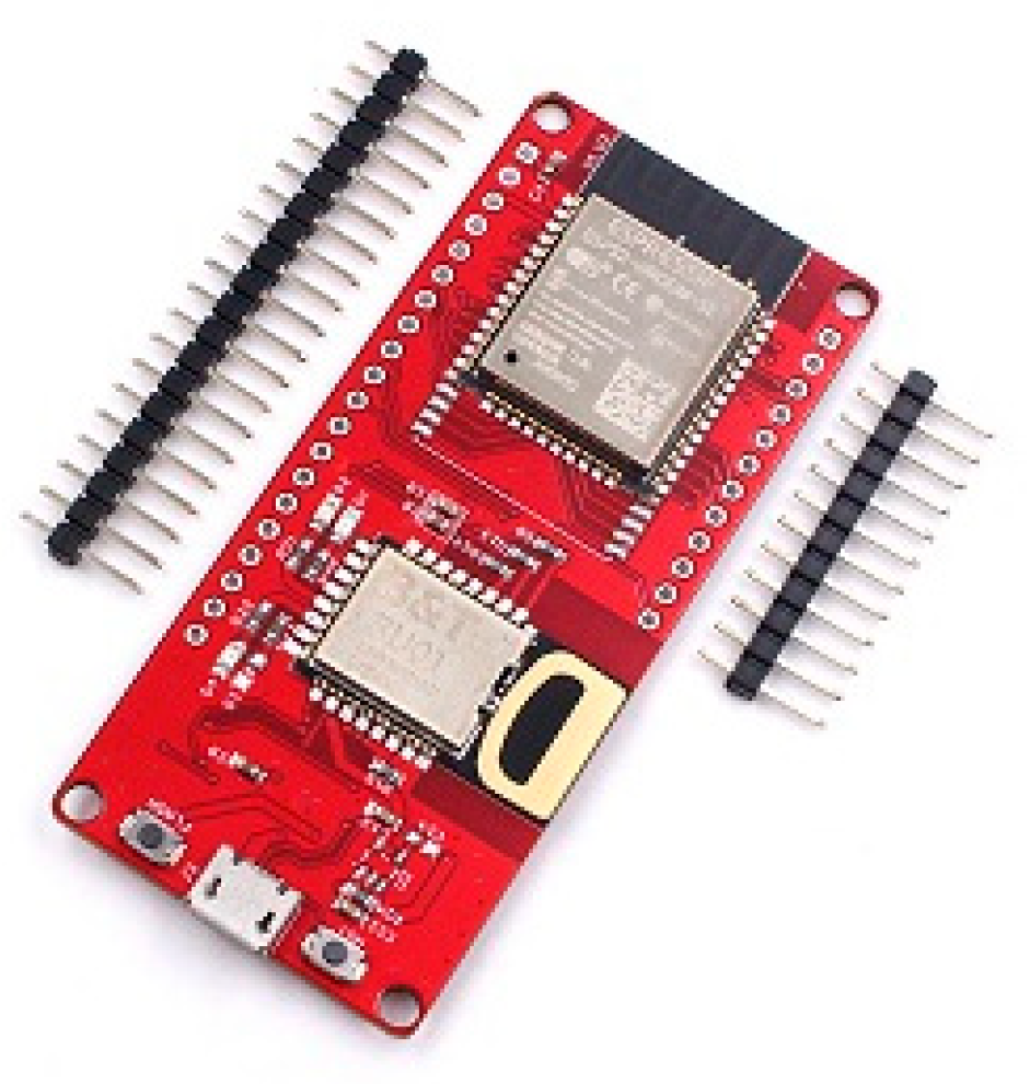
This study utilizes the Makerfabs ESP32 UWB module, as shown in Figure 1. Based on the DW1000, it functions like a continuous scanning radar, capable of precisely locking onto another device (referred to as an Anchor) and communicating with it to calculate its position. It employs the ESP32-WROOM/WROVE central processing unit manufactured by Espressif Systems Co., Ltd. (Shanghai, China) and offers a maximum ranging distance of 45 m. Once the device is in proximity to another UWB device, it begins ranging through bi-directional two-way ranging (TWR).

2.2. Line-of-Sight and Non-Line-of-Sight Channels

LOS and NLOS channels are two fundamental conditions in wireless communication systems that affect signal propagation and reception quality. In LOS channels, there is a direct, unobstructed path from the transmitter to the receiver, typically providing the best communication quality and the least signal attenuation. In contrast, in NLOS channels, the signal may encounter various obstacles (such as buildings, trees, or other objects) before reaching the receiver, leading to increased signal attenuation, scattering, diffraction, or reflection, thereby affecting the reliability and accuracy of communication.

The impact of LOS and NLOS channels on UWB indoor positioning systems is significant, mainly reflected in positioning accuracy and reliability. In LOS channels, the UWB signal is transmitted directly from the transmitter to the receiver without any obstacles, typically offering the best positioning accuracy and minimal signal attenuation. On the other hand, in NLOS channels, due to the presence of walls, furniture, or other obstacles that block or reflect the UWB signal, signal attenuation, scattering, and multipath effects occur. These effects often impact the signal’s time of arrival, thus reducing positioning accuracy and increasing positioning errors. Therefore, understanding and addressing these channels are crucial for enhancing the performance of UWB indoor positioning systems. Common technical strategies include using Kalman filters to restore signal variations caused by NLOS channels and deploying multiple receivers to reduce the impact of NLOS channels on the system.

2.3. Ranging Principle

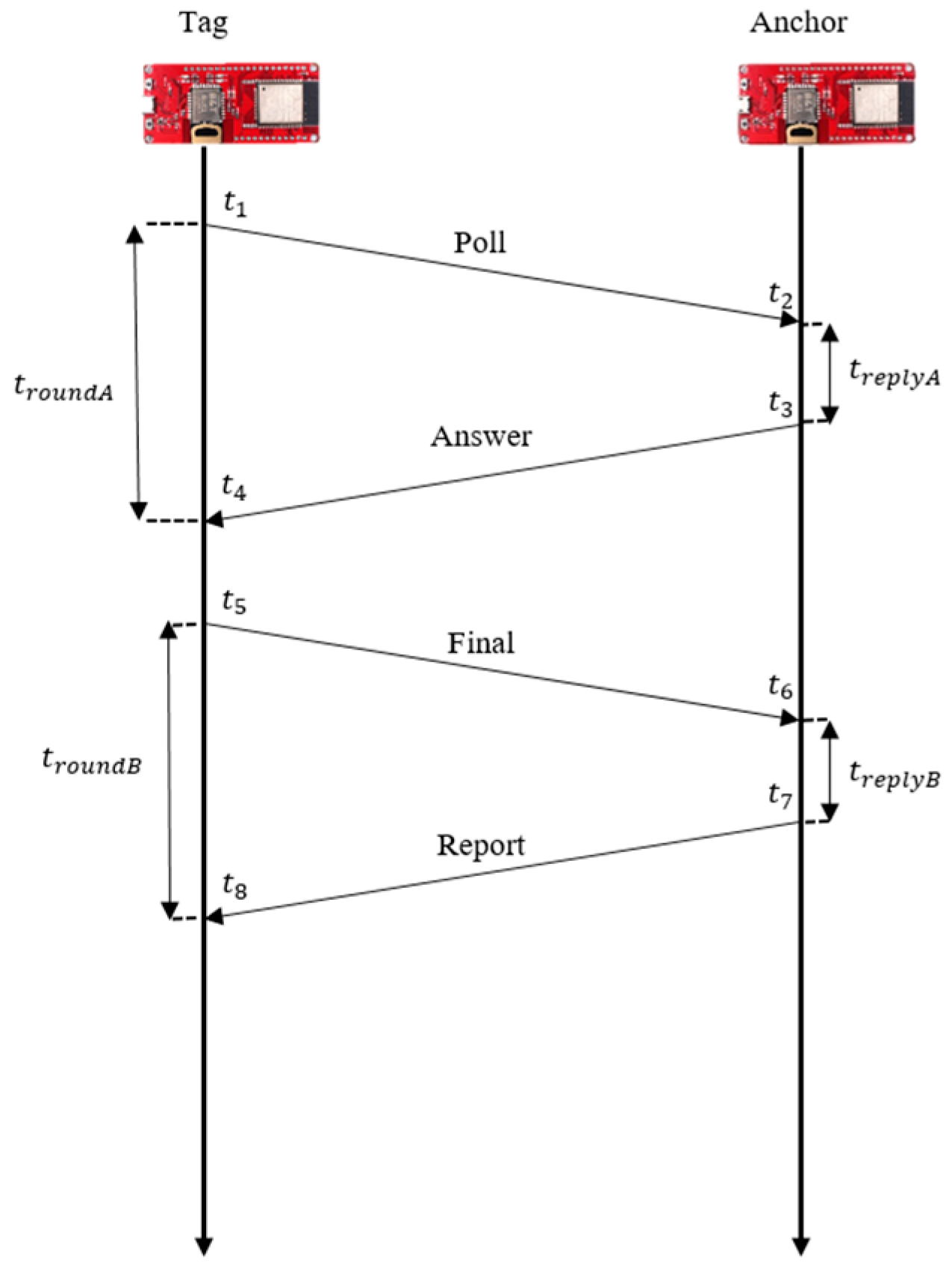
TWR is a technique used in wireless communication to measure the distance between two devices, applicable to wireless systems such as UWB. This method involves two devices alternately sending and receiving signals, thereby calculating the total round-trip time of the signals [28], as shown in Figure 2. In the process of bi-directional two-way ranging, initially, one device (commonly referred to as the transmitter) sends a signal to another device (the receiver). After receiving the signal, the receiver sends another signal back after a certain delay time. When the original transmitter receives this return signal, it can calculate the total time taken for the signal to be sent and received. By multiplying this time by the speed of signal propagation (such as the speed of light), the distance can be calculated.

Bi-directional TWR is a method that uses wireless communication technology to measure the distance between two devices, involving alternating signal transmission and reception between the two devices. In Figure 3, there are two devices, a tag and an anchor, which engage in multiple signal exchanges to calculate the distance between them. The terms $t_{roundA}=t_4-t_1$ and $t_{roundB}=t_3-t_6$ represent the signal propagation time—that is, the time it takes for the signal to travel from one device to another. The terms $t_{replyA}=t_3-t_2$ and $t_{replyB}=t_7-t_6$ represent the time taken by the anchor to send a response signal after receiving the poll and final signals, respectively. The signal flight time $t_{prop}$ can be represented by

$$t_{prop}={\displaystyle \frac{t_{roundA}+t_{roundB}-t_{replayA}-t_{replayB}}{4}}$$

(1)

The distance d can then be represented as

$$d=t_{prop}\times c$$

(2)

where c represents the speed of light ($3\times {10}^8$ m/s). TWR is widely used across various fields due to its ability to provide direct and accurate distance measurements, such as in obstacle detection for autonomous vehicles, 3D imaging, robotic navigation, and interactive entertainment systems.

2.4. Three-Dimensional Spatial Positioning Methods

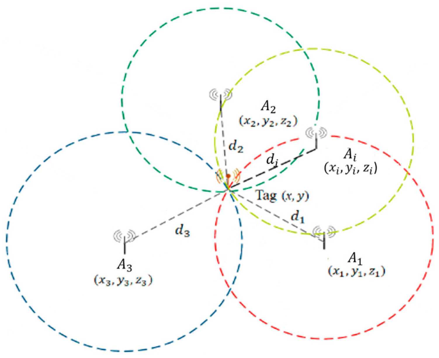
The proposed localization framework enables three-dimensional positioning using multiple reference anchors. To resolve an unambiguous position in three-dimensional space, a minimum of four anchors with known spatial coordinates is necessary. After obtaining the range measurements between the target tag and the anchors, expressed as ($d_i, i=1, 2, \cdots , M$), geometric constraints are formed in space. For the representative case where $M=4$, four distance-based geometric loci are generated, as illustrated in Figure 4. The spatial point that simultaneously satisfies all four constraints is identified as the estimated position of the target tag.

Let the coordinates of the UWB anchor points be represented as ${\mathrm{A}}_1$($x_1,y_1,z_1$), ${\mathrm{A}}_2$($x_2,y_2,z_2$), ${\mathrm{A}}_3$($x_3,y_3,z_3$) …${\mathrm{A}}_i$ ($x_i,y_i,z_i$)… ${\mathrm{A}}_M$($x_M,y_M,z_M$). The coordinates of the tag are represented as (x, y, z). Let ${\widehat{d}}_1,{\widehat{d}}_2, {\widehat{d}}_3$… ${\widehat{d}}_i$ represent the i-th estimated distances from the tag to each anchor point. Consider a set of M UWB anchors whose fixed spatial positions are given by $A_i=\left(x_i, y_i, z_i\right), i=1, 2, \cdots , M$. The three-dimensional location of the target node is described by the unknown vector $(x, y, z)$. Let $d_i$ denote the range estimate associated with the signal path between the target and the i-th anchor. These range observations impose distance constraints between the unknown target position and the known anchor coordinates, from which the localization model is constructed as follows:

$$\{\begin{array}{c}\sqrt{{\left(\widehat{x}-x_1\right)}^2+{\left(\widehat{y}-y_1\right)}^2+{\left(\widehat{z}-z_1\right)}^2}={\widehat{d}}_1\\ \sqrt{{\left(\widehat{x}-x_2\right)}^2+{\left(\widehat{y}-y_2\right)}^2+{\left(\widehat{z}-z_2\right)}^2}={\widehat{d}}_2\\ \sqrt{{\left(\widehat{x}-x_3\right)}^2+{\left(\widehat{y}-y_3\right)}^2+{\left(\widehat{z}-z_3\right)}^2}={\widehat{d}}_3\\ \dots \\ \sqrt{{\left(\widehat{x}-x_M\right)}^2+{\left(\widehat{y}-y_M\right)}^2+{\left(\widehat{z}-z_M\right)}^2}={\widehat{d}}_M\end{array}$$

(3)

After organizing, a system of linear equations (Equation (4)) can be obtained:

$$\{\begin{array}{l}2\widehat{x}\left(x_2-x_1\right)+2\widehat{y}\left(y_2-y_1\right)+2\widehat{z}\left(z_2-z_1\right)\\ ={\widehat{d}}_1^2-{\widehat{d}}_2^2+x_2^2-x_1^2+y_2^2-y_1^2+z_2^2-z_1^2\\ 2\widehat{x}\left(x_3-x_1\right)+2\widehat{y}\left(y_3-y_1\right)+2\widehat{z}\left(z_3-z_1\right)\\ ={\widehat{d}}_1^2-{\widehat{d}}_3^2+x_3^2-x_1^2+y_3^2-y_1^2+z_3^2-z_1^2\\ \hfill \dots \hfill \\ 2\widehat{x}\left(x_M-x_1\right)+2\widehat{y}\left(y_M-y_1\right)+2\widehat{z}\left(z_M-z_1\right)\\ ={\widehat{d}}_1^2-{\widehat{d}}_M^2+x_M^2-x_1^2+y_M^2-y_1^2+z_M^2-z_1^2\end{array}$$

(4)

Then, by organizing the aforementioned equations and utilizing matrix calculations, the three-dimensional coordinates of the tag can be obtained as follows:

$$\mathbf{X}\widehat{\mathbf{b}}=\mathbf{w},$$

(5)

where

$$\mathbf{X}=\left[\begin{array}{c}\begin{array}{ccc}2\left(x_2-x_1\right)& 2\left(y_2-y_1\right)& 2\left(z_2-z_1\right)\\ 2\left(x_3-x_1\right)& 2\left(y_3-y_1\right)& 2\left(z_3-z_1\right)\end{array}\\ \begin{array}{ccc}& \dots & \\ 2\left(x_M-x_1\right)& 2\left(y_M-y_1\right)& 2\left(z_M-z_1\right)\end{array}\end{array}\right],$$

(6)

$$\widehat{\mathbf{b}}=\left[\begin{array}{c}\widehat{x}\\ \widehat{y }\\ \widehat{z}\end{array}\right],$$

(7)

and

$$\mathbf{w}=\left[\begin{array}{c}\begin{array}{c}\begin{array}{c}{\widehat{d}}_1^2-{\widehat{d}}_2^2+x_2^2+y_2^2+z_2^2-x_1^2-y_1^2-z_1^2\\ {\widehat{d}}_1^2-{\widehat{d}}_3^2+x_3^2+y_3^2+z_3^2-x_1^2-y_1^2-z_1^2\end{array}\\ \dots \end{array}\\ \begin{array}{c}{\widehat{d}}_1^2-{\widehat{d}}_{\mathrm{M}}^2+x_{\mathrm{M}}^2+y_{\mathrm{M}}^2+z_M^2-x_1^2-y_1^2-z_1^2\end{array}\end{array}\right].$$

(8)

Through the operation of the matrices, the coordinates of the point to be located ($\widehat{x}, \widehat{y}, \widehat{z}$) are determined by solving for the matrix $\widehat{\mathbf{b}}$. If the inverse of matrix ${\mathbf{X}}^{\mathrm{T}}\mathbf{X}$ exists, solving Equation (5) yields

$${\mathbf{X}}^{\mathrm{T}}\mathbf{X}\times \widehat{\mathbf{b}}={\mathbf{X}}^{\mathrm{T}}\times \mathbf{w}\mathbf{.}$$

(9)

The result can be organized as follows:

$${\left({\mathbf{X}}^{\mathrm{T}}\mathbf{X}\right)}^{-1}\times {\mathbf{X}}^{\mathrm{T}}\mathbf{X}\times \widehat{\mathbf{b}}={\left({\mathbf{X}}^{\mathrm{T}}\mathbf{X}\right)}^{-1}\times {\mathbf{X}}^{\mathrm{T}}\times \mathbf{w}$$

(10)

where the transpose of matrix X is presented as ${\mathbf{X}}^{\mathrm{T}}$. The coordinates of the tags can be determined as follows:

$$\widehat{\mathbf{b}} =\left[\begin{array}{c}\widehat{x}\\ \widehat{y}\\ \widehat{z}\end{array}\right]= {{(\mathbf{X}}^{\mathrm{T}}\mathbf{X})}^{-1}{\mathbf{X}}^{\mathrm{T}}\mathbf{w}$$

(11)

2.5. Particle Swarm Optimization

PSO is a representative swarm-based optimization technique originally introduced by Kennedy and Eberhart in 1995 [30,31]. The algorithm is motivated by observations of collective search behaviors in natural groups, such as bird flocks, where individuals exploit both self-acquired knowledge and information exchanged within the group to reach favorable locations.

In PSO, the optimization problem is explored within a $d$-dimensional search space populated by n candidate solutions, referred to as particles. Each particle corresponds to a potential solution, whose state is described by a position vector ${\mathbf{X}}_{id}=\left(x_{i1},x_{i2},\dots , x_{id}\right)$ and an associated velocity vector ${\mathbf{V}}_{id}=\left(v_{i1}, v_{i2}, \cdots , v_{id}\right)$.

During the iterative search process, particles evaluate their fitness values to record two key reference states: the best position previously attained by the particle itself, denoted as ${\mathbf{X}}_{id,pbest}(x_{i1}, x_{i2}, \cdots , x_{id})$, and the best position discovered by the entire swarm, denoted as ${\mathbf{X}}_{id,gbest}\left(x_{1,gbest},x_{2,gbest},\dots ,x_{d,gbest}\right)$. The search dynamics of PSO are governed by the balance between individual learning and social cooperation. Specifically, particle trajectories are adjusted according to both the particle’s own historical best experience and the collective knowledge of the swarm. Under this mechanism, particle velocities are updated as follows:

$${\mathbf{V}}_{id}^{k+1}=w\left(k\right){\mathbf{V}}_{id}^{k+1}+r_1{c}_1\left({\mathbf{X}}_{id,pbest}^k-{\mathbf{X}}_{id}^k\right)+r_2{c}_2\left({\mathbf{X}}_{id,gbest}^k-{\mathbf{X}}_{id}^k\right),$$

(12)

where $k$ denotes the iteration index. The coefficients $c_1$ and $c_2$ represent the cognitive and social learning parameters, respectively, while $r_1$ and $r_2$ are independent random variables uniformly distributed in the interval $[0,1]$, introducing stochastic diversity into the search behavior. The inertia weight $w\left(k\right)$ controls the influence of the previous velocity and is employed in this study to suppress excessive velocity growth and enhance algorithmic stability.

To regulate the exploration trade-off, a linearly decreasing inertia strategy is adopted, given by

$$w\left(k\right)=w_{max}-{\displaystyle \frac{w_{max}-w_{min}}{k_{max}}}\times k,$$

(13)

where $w_{max}$ and $w_{min}$ denote the upper and lower bounds of the inertia weight, respectively, and $k_{max}$ is the predefined maximum number of iterations. This adaptive adjustment encourages extensive global exploration in early iterations and progressively emphasizes local refinement as convergence proceeds.

Finally, particle positions are updated according to

$${\mathbf{X}}_{id}^{k+1}={\mathbf{X}}_{id}^k+{\mathbf{V}}_{id}^{k+1},$$

(14)

thus completing one iteration of the PSO search process.

3. Multi-Anchor Indoor Positioning Experiments

To enhance the accuracy of UWB indoor positioning technology in three-dimensional space, this study employs a multi-anchor system for positioning experiments. This section provides a detailed introduction to the experimental setup, including the detailed layout of the experimental environment, the equipment used, and the technical parameters, as well as each step of the experimental process. Additionally, this section analyzes the experimental data to explore the specific impact of multi-anchor configurations on improving the precision of UWB indoor positioning.

3.1. Ranging Experiments

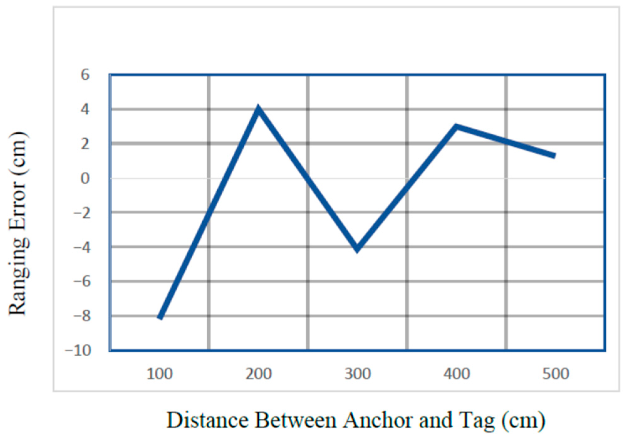
This ranging experiment utilized one anchor and one tag, testing at five different distances between the anchor and the tag (100 cm, 200 cm, 300 cm, 400 cm, 500 cm). To minimize the impact of angles on the ranging results, the measurements were conducted face-to-face between the anchor and the tag. Each testing point underwent 1000 measurements, and the results are shown in Figure 5. In Figure 5, the error values for distances of 100 cm to 500 cm between the anchor and the tag are −8.2, 4, −4.1, 3, and 1.3 cm, respectively.

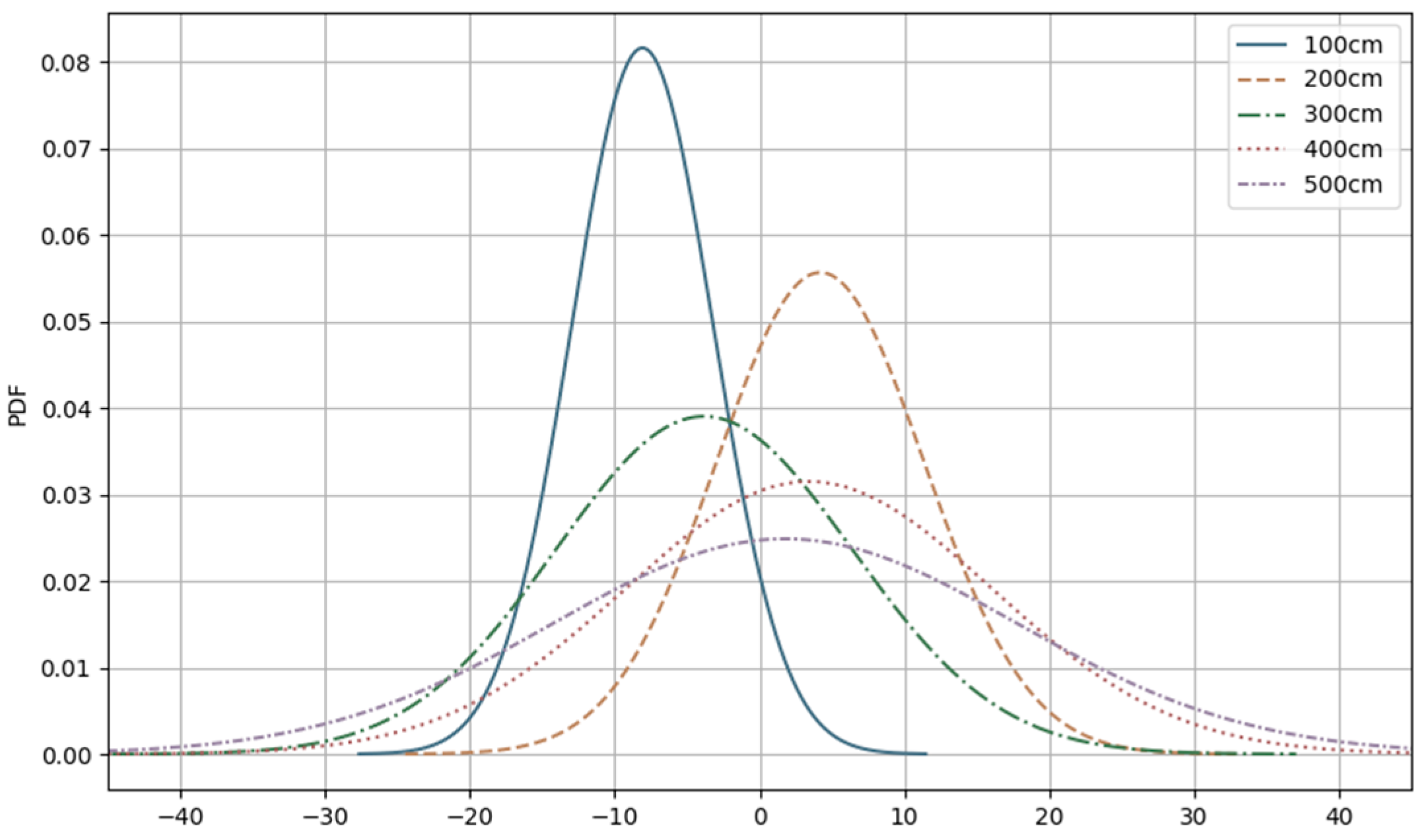
Figure 6 shows the probability density function (PDF) plots of ranging error value distributions for each test distance in the ranging experiment. The width of the distribution reflects the variance characteristics of the errors. The standard deviation distributions at 500 cm and 400 cm are wider, indicating greater variability in errors at these distances. The standard deviation distribution at 100 cm is narrower, indicating less error variability.

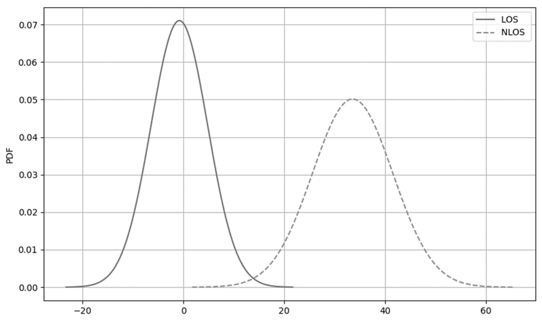
Figure 7 presents the distribution of ranging errors under LOS and NLOS conditions at different distances. In the figure, the solid line represents the error distribution under LOS conditions, while the dashed line represents the error distribution under NLOS conditions. In the LOS channel, the error distribution is symmetrically narrow and peaked, concentrated around 0 cm with a standard deviation range of about 8 cm. This shows that, under LOS conditions, measurement errors are very small, location estimation is highly precise, and the error distribution is more concentrated. In contrast, the NLOS channel, due to unstable signal transmission, shows a wider error distribution with a peak at about 32 cm and a standard deviation range of about 12 cm. This indicates that under NLOS conditions, measurement errors are larger and more pronounced, increasing the uncertainty in location estimation. Moreover, the error values in NLOS channels vary due to differences in obstructions. Therefore, based on the standard deviation of ranging measurements in a ranging experiment, the LOS and NLOS channels can be decided.

3.2. Multi-Anchor Positioning Experimental Environment

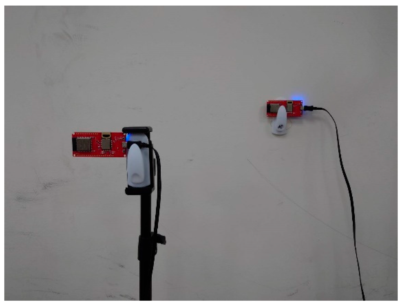
The experimental measurements were carried out in Room 209.1 of the Information Building at Chaoyang University of Technology. During the tests, fixed anchor nodes transmitted signals to mobile tags, which measured distances using the TWR method and transmitted the data to a local processing system for subsequent positioning computations. To ensure consistency across repeated trials, the anchors were mounted on the walls using hooks, minimizing the potential for human-induced positioning errors. The tags were placed on adjustable tripods to facilitate flexible relocation between measurement points, as illustrated in Figure 8.

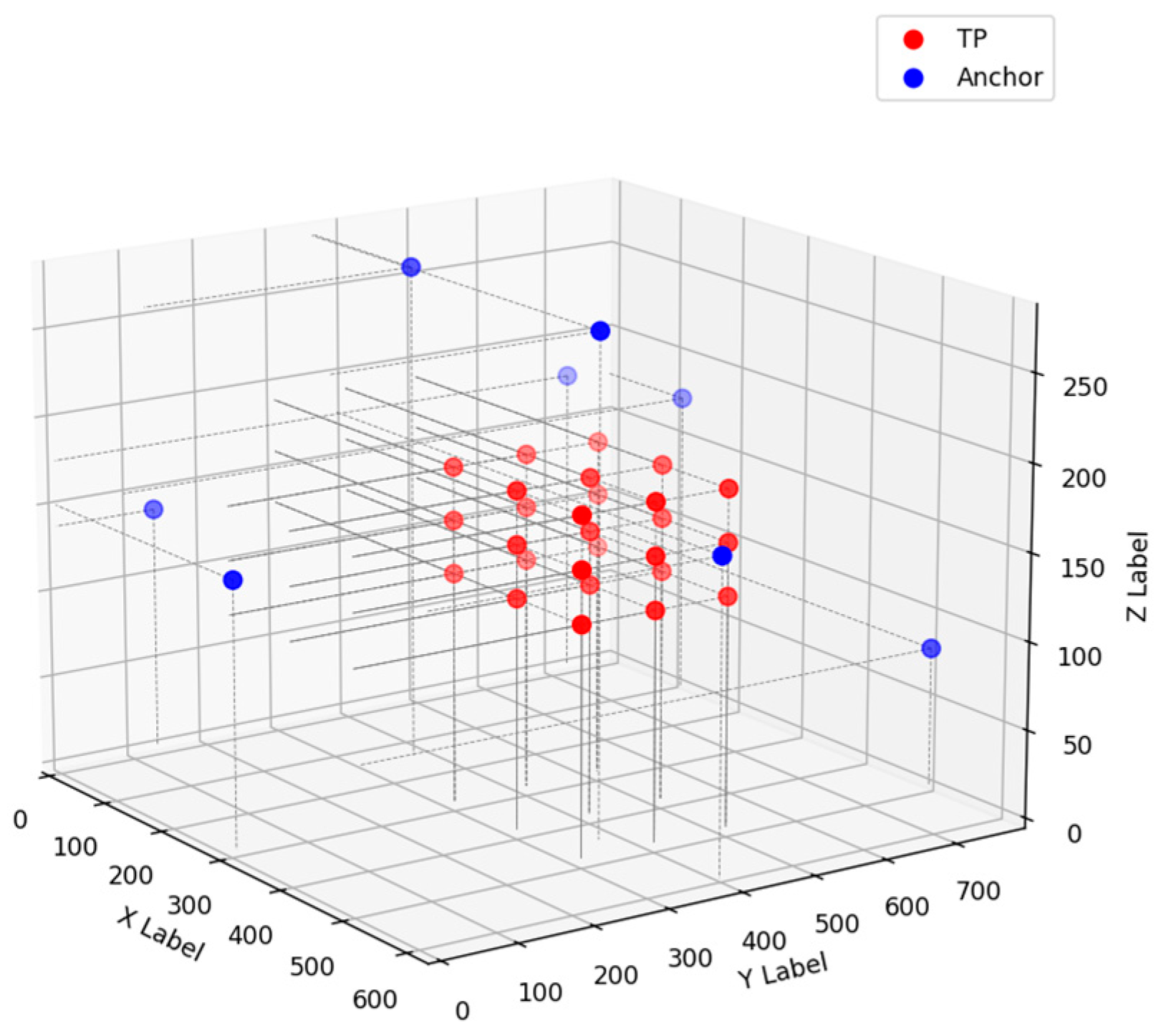
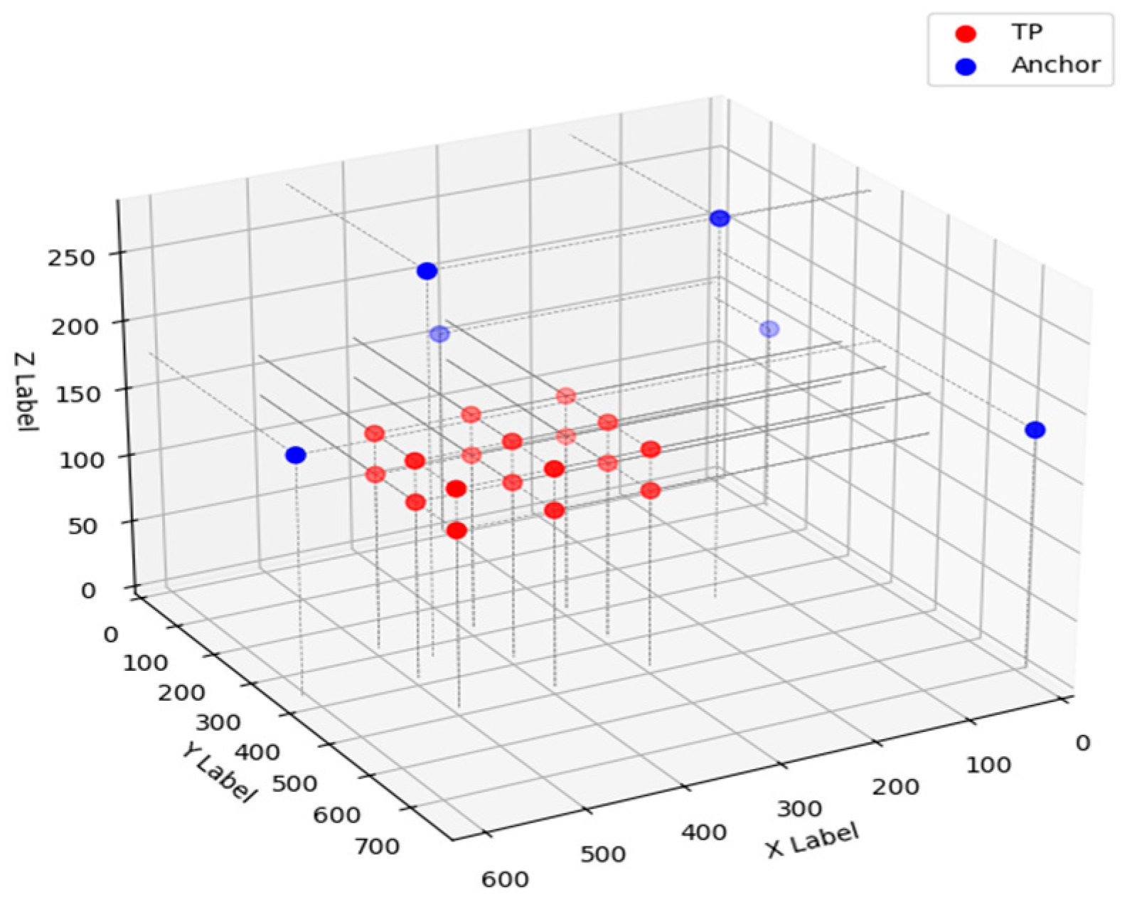
To maintain experimental accuracy, all anchors except the eighth were deployed under LOS conditions. The measurements were performed within a three-dimensional space measuring 620 cm × 783 cm × 282 cm, as depicted in Figure 9. A total of eight anchors were employed, indicated by blue markers in the figure, with their precise spatial coordinates provided in

Table 1. Coordinates of eight anchors (unit: m).

Anchor	x	y	z
${\mathrm{A}}_1$	6.14	3.86	1.77
${\mathrm{A}}_2$	0.00	1.32	1.38
${\mathrm{A}}_3$	0.00	7.22	1.76
${\mathrm{A}}_4$	1.63	3.58	2.82
${\mathrm{A}}_5$	4.66	3.55	2.82
${\mathrm{A}}_6$	3.07	0.00	1.50
${\mathrm{A}}_7$	1.22	7.83	1.73
${\mathrm{A}}_8$	5.09	7.83	0.80

. The experiment utilized a single tag, and 27 designated test points (TPs) were selected for evaluation, shown as red markers in Figure 9. The coordinates corresponding to these test points are summarized in

Table 2. Three-dimensional locations of test nodes under multi-anchor configurations.

	Coordinate		(Unit: m) y			Coordinate		(Unit: m) y
TP		x		z	TP		x		z
${\mathrm{T}\mathrm{P}}_{\mathrm{A}1}$		3.0	3.0	1.3	${\mathrm{T}\mathrm{P}}_{\mathrm{E}3}$		4.0	4.0	1.9
${\mathrm{T}\mathrm{P}}_{\mathrm{A}2}$		3.0	3.0	1.6	${\mathrm{T}\mathrm{P}}_{\mathrm{F}1}$		5.0	4.0	1.3
${\mathrm{T}\mathrm{P}}_{\mathrm{A}3}$		3.0	3.0	1.9	${\mathrm{T}\mathrm{P}}_{\mathrm{F}2}$		5.0	4.0	1.6
${\mathrm{T}\mathrm{P}}_{\mathrm{B}1}$		4.0	3.0	1.3	${\mathrm{T}\mathrm{P}}_{\mathrm{F}3}$		5.0	4.0	1.9
${\mathrm{T}\mathrm{P}}_{\mathrm{B}2}$		4.0	3.0	1.6	${\mathrm{T}\mathrm{P}}_{\mathrm{G}1}$		3.0	5.0	1.3
${\mathrm{T}\mathrm{P}}_{\mathrm{B}3}$		4.0	3.0	1.9	${\mathrm{T}\mathrm{P}}_{\mathrm{G}2}$		3.0	5.0	1.6
${\mathrm{T}\mathrm{P}}_{\mathrm{C}1}$		5.0	3.0	1.3	${\mathrm{T}\mathrm{P}}_{\mathrm{G}3}$		3.0	5.0	1.9
${\mathrm{T}\mathrm{P}}_{\mathrm{C}2}$		5.0	3.0	1.6	${\mathrm{T}\mathrm{P}}_{\mathrm{H}1}$		4.0	5.0	1.3
${\mathrm{T}\mathrm{P}}_{\mathrm{C}3}$		5.0	3.0	1.9	${\mathrm{T}\mathrm{P}}_{\mathrm{H}2}$		4.0	5.0	1.6
${\mathrm{T}\mathrm{P}}_{\mathrm{D}1}$		3.0	4.0	1.3	${\mathrm{T}\mathrm{P}}_{\mathrm{H}3}$		4.0	5.0	1.9
${\mathrm{T}\mathrm{P}}_{\mathrm{D}2}$		3.0	4.0	1.6	${\mathrm{T}\mathrm{P}}_{\mathrm{I}1}$		5.0	5.0	1.3
${\mathrm{T}\mathrm{P}}_{\mathrm{D}3}$		3.0	4.0	1.9	${\mathrm{T}\mathrm{P}}_{\mathrm{I}2}$		5.0	5.0	1.6
${\mathrm{T}\mathrm{P}}_{\mathrm{E}1}$		4.0	4.0	1.3	${\mathrm{T}\mathrm{P}}_{\mathrm{I}3}$		5.0	5.0	1.9
${\mathrm{T}\mathrm{P}}_{\mathrm{E}2}$		4.0	4.0	1.6

.

3.3. Results of Multi-Anchor Positioning Experiment

In this experiment, we conducted 1000 individual measurements for each test point (TP). The 3D average positioning error $\overline{{\epsilon }_i}$ for ${\mathrm{T}\mathrm{P}}_i$, as listed in

Table 3. Multi-anchor experiment results.

	Experiment	4A	5A	6A	7A	8A		Experiment	4A	5A	6A	7A	8A
TP							TP
${\mathrm{T}\mathrm{P}}_{\mathrm{A}1}$		17.2	8.0	7.9	11.7	10.4	${\mathrm{T}\mathrm{P}}_{\mathrm{E}3}$		15.7	19.1	17.2	17.5	15.0
${\mathrm{T}\mathrm{P}}_{\mathrm{A}2}$		9.1	6.9	6.7	7.9	11.6	${\mathrm{T}\mathrm{P}}_{\mathrm{F}1}$		7.9	9.5	8.8	9.1	11.5
${\mathrm{T}\mathrm{P}}_{\mathrm{A}3}$		13.6	9.5	7.3	8.9	17.8	${\mathrm{T}\mathrm{P}}_{\mathrm{F}2}$		14.1	11.0	10.6	10.0	11.7
${\mathrm{T}\mathrm{P}}_{\mathrm{B}1}$		14.1	8.7	5.8	3.7	7.6	${\mathrm{T}\mathrm{P}}_{\mathrm{F}3}$		17.2	6.6	6.4	8.9	12.7
${\mathrm{T}\mathrm{P}}_{\mathrm{B}2}$		22.7	11.2	8.6	11.7	15.5	${\mathrm{T}\mathrm{P}}_{\mathrm{G}1}$		9.8	10.3	5.7	7.3	12.2
${\mathrm{T}\mathrm{P}}_{\mathrm{B}3}$		21.6	7.8	6.9	7.2	8.4	${\mathrm{T}\mathrm{P}}_{\mathrm{G}2}$		13.1	10.3	12.7	9.0	10.0
${\mathrm{T}\mathrm{P}}_{\mathrm{C}1}$		13.1	13.0	9.6	7.3	33.6	${\mathrm{T}\mathrm{P}}_{\mathrm{G}3}$		9.1	10.1	6.5	6.7	11.2
${\mathrm{T}\mathrm{P}}_{\mathrm{C}2}$		10.0	4.9	3.9	3.1	18.9	${\mathrm{T}\mathrm{P}}_{\mathrm{H}1}$		15.8	21.3	7.2	6.3	6.6
${\mathrm{T}\mathrm{P}}_{\mathrm{C}3}$		16.3	7.5	4.8	5.4	16.9	${\mathrm{T}\mathrm{P}}_{\mathrm{H}2}$		16.7	9.8	7.5	6.5	5.4
${\mathrm{T}\mathrm{P}}_{\mathrm{D}1}$		7.0	5.0	5.8	4.7	4.9	${\mathrm{T}\mathrm{P}}_{\mathrm{H}3}$		19.5	19.4	14.0	13.1	11.4
${\mathrm{T}\mathrm{P}}_{\mathrm{D}2}$		12.3	12.3	12.4	12.1	8.2	${\mathrm{T}\mathrm{P}}_{\mathrm{I}1}$		15.4	8.7	6.6	7.4	8.8
${\mathrm{T}\mathrm{P}}_{\mathrm{D}3}$		16.3	11.1	9.8	10.3	16.5	${\mathrm{T}\mathrm{P}}_{\mathrm{I}2}$		11.8	14.7	12.5	13.7	11.7
${\mathrm{T}\mathrm{P}}_{\mathrm{E}1}$		6.2	7.0	7.3	11.5	19.1	${\mathrm{T}\mathrm{P}}_{\mathrm{I}3}$		20.5	8.6	7.6	8.2	16.2
${\mathrm{T}\mathrm{P}}_{\mathrm{E}2}$		10.4	11.7	9.8	9.2	7.2	AVG		13.9	10.5	8.5	8.8	12.6

, is as follows:

$$\overline{{\epsilon }_i}={\displaystyle \frac{\sum _{n=1}^N\sqrt{{{(x}_{i,n}-{\widehat{x}}_{i,n})}^2+{(y_{i,n}-{\widehat{y}}_{i,n})}^2+{(z_{i,n}-{\widehat{z}}_{i,n})}^2}}{N}}$$

(15)

In this experiment, $x_{i,n}$, $y_{i,n}$, and $z_{i,n}$ denote the true X, Y, and Z coordinates of the i-th test point, while ${\widehat{x}}_{i,n}$, ${\widehat{y}}_{i,n}$, and ${\widehat{z}}_{i,n}$ represent the corresponding estimated coordinates. For each TP, a total of $N=1000$ measurements were collected. The three-dimensional positioning tests were conducted using 4, 5, 6, 7, and 8 anchors, with the anchors sequentially added from $A_1$ to $A_8$. The full set of experimental results is presented in Table 3.

Analysis of Table 3 shows that the maximal positioning error occurs at $T{P}_{B2}$ with 22.7 cm, while the minimal error of 6.2 cm is observed at $T{P}_{E11}$. Table 3 also provides the overall average positioning errors for each anchor configuration, offering a comprehensive assessment of system performance. The average errors for 4, 5, 6, 7, and 8 anchors are 13.9, 10.5, 8.5, 8.8, and 12.6 cm, respectively, indicating that increasing the number of anchors generally improves localization accuracy. However, the relatively high error observed with eight anchors is attributed to $A_8$ being located in an NLOS channel relative to the test points. Similarly, the slightly higher error for seven anchors compared to six arises because $A_7$ is positioned near the edge of the measurement area; its larger angular spread relative to the test points contributes to increased ranging errors.

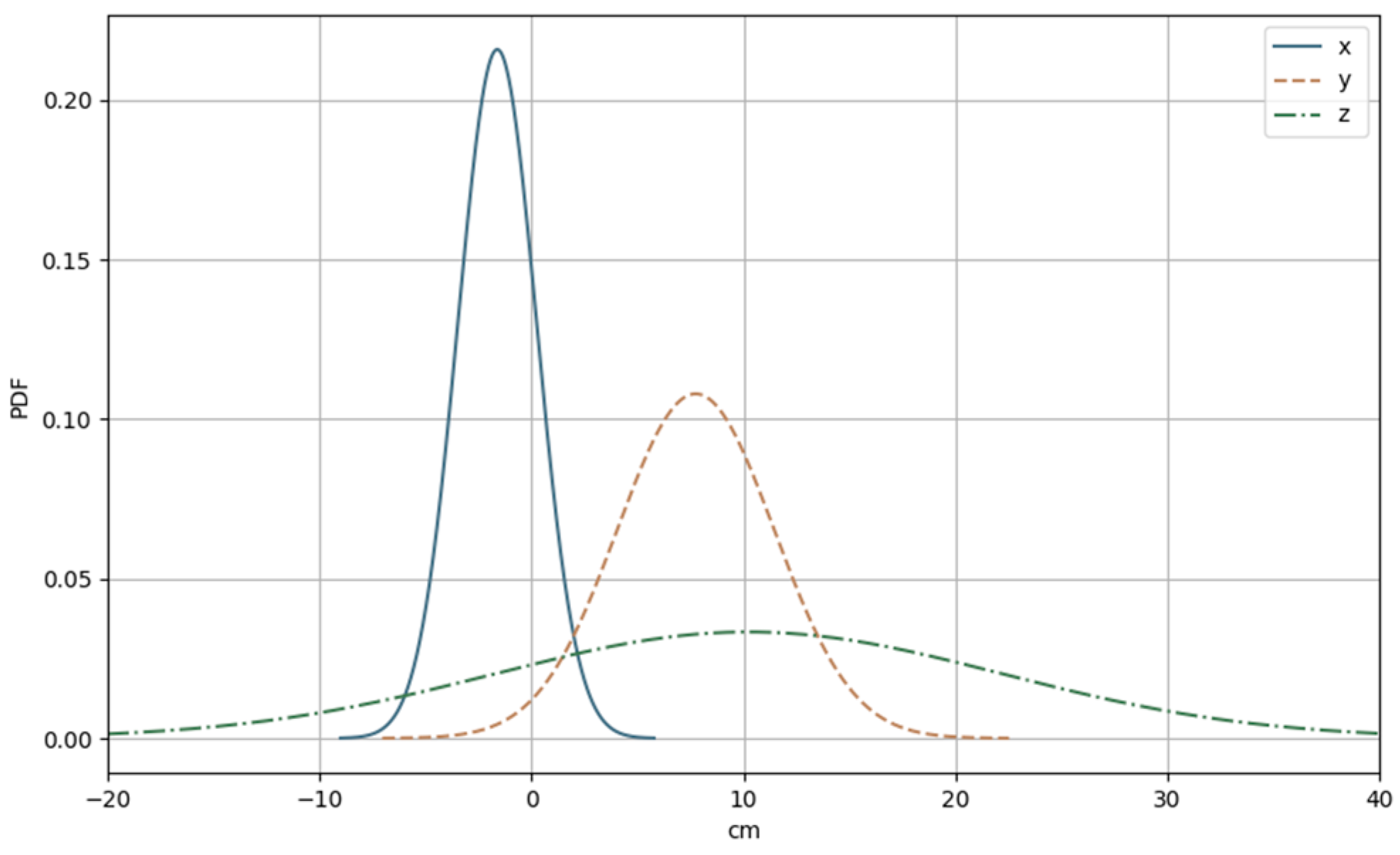
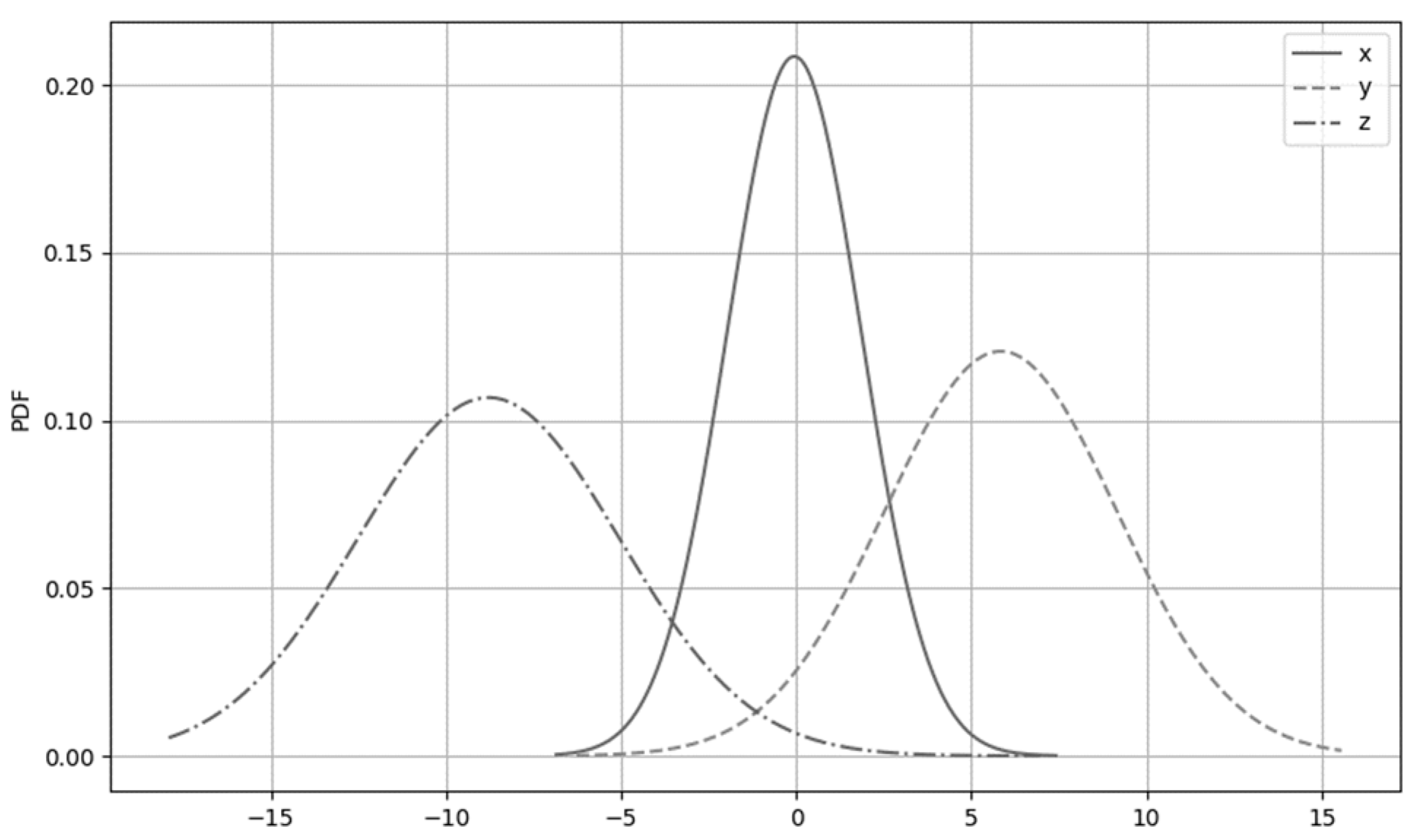
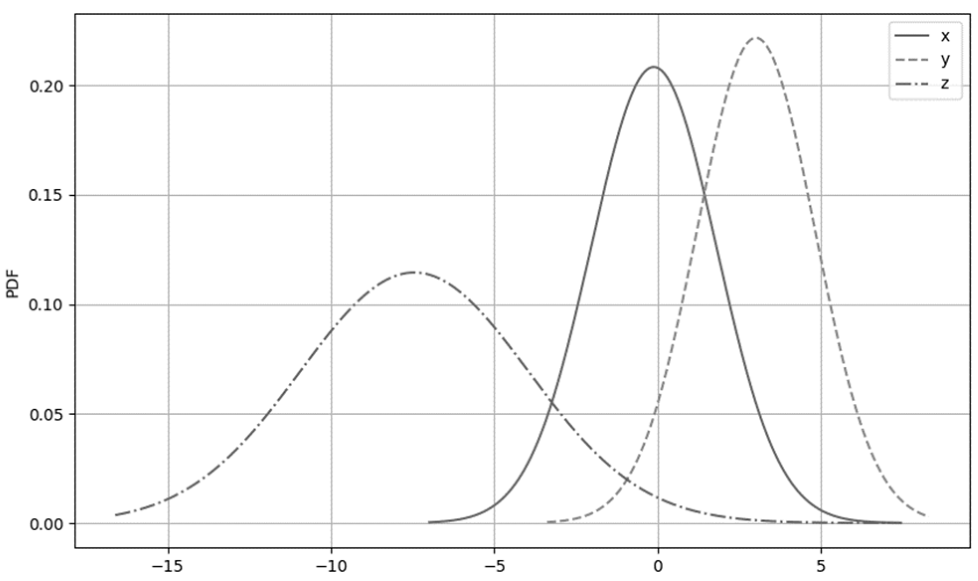
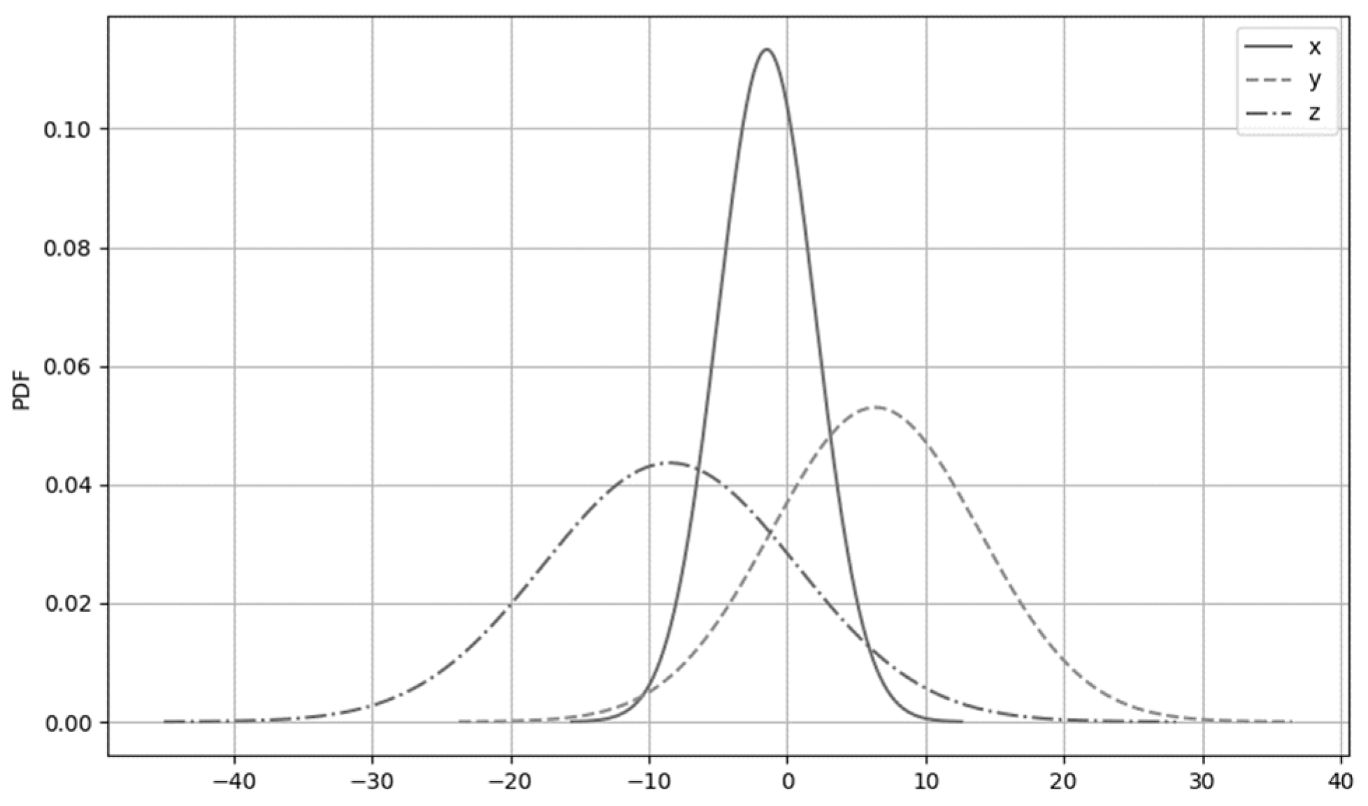
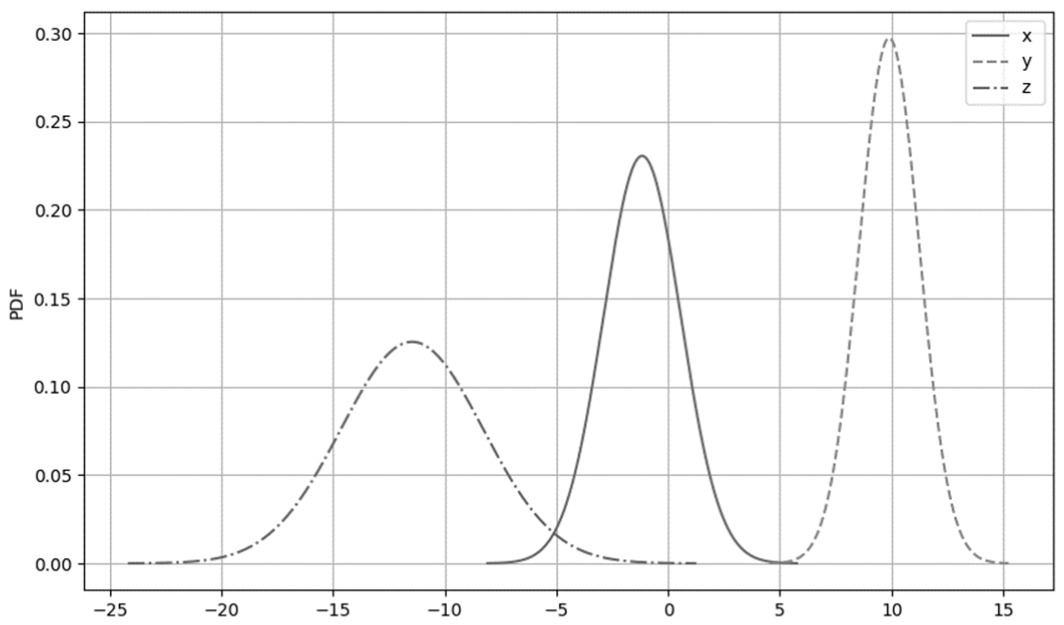
Figure 10, Figure 11, Figure 12, Figure 13 and Figure 14 show the PDF of the positioning error ${\mathrm{T}\mathrm{P}}_{\mathrm{B}2}$ with 4A, 5A, 6A, 7A, and 8A, respectively. In Figure 10, during the 4A experiment for TP_B2, the error PDFs for x, y, and z show that the error for x is about −1 cm, that for y is 9 cm, and that for z is −20 cm. It is evident from the figure that the error and distribution on the z-axis are significantly larger than those on the other axes, which may be due to the small z-axis errors among the anchors in our experimental environment, leading to larger calculated errors for the z-axis in the positioning equations.

In Figure 11, Figure 12, Figure 13 and Figure 14, as more anchor points are added, the error values and distributions for all three axes become smaller, demonstrating that multi-anchor positioning not only reduces the error values but also increases positioning stability.

In Figure 13, with the addition of ${\mathrm{A}}_7$, which is positioned at the edge of the positioning environment, the error values on all three axes increased from the original 0, 4, and 7 cm to −1, 9, and −9 cm, respectively. This increase in error can be attributed to ${\mathrm{A}}_7$’s edge location, which affects the angular measurements and contributes to larger errors due to the angles involved.

Figure 14 incorporates ${\mathrm{A}}_8$, which is situated on an NLOS channel. The inclusion of ${\mathrm{A}}_8$ leads to a significant increase in both the error values and error distribution. This is because NLOS conditions typically introduce disruptions in signal propagation, such as reflections, diffractions, and scattering, which, in turn, increase measurement inaccuracies and variability in the data collected.

3.4. Experiment on the Impact of NLOS on Multi-Anchor Positioning

From the experimental results in the previous section, it can be observed that, when all anchor points are in LOS conditions, the addition of even one NLOS anchor significantly increases the error in the positioning system. To gain a deeper understanding of the impact of NLOS channels on the accuracy of multi-anchor positioning systems, this section presents four specifically designed experimental configurations. These experiments will explore, in detail, how the number of anchor points in NLOS channels affects the overall positioning accuracy, with the aim of providing more precise system design and optimization recommendations.

This section covers four experimental designs aimed at observing the impact of NLOS channels on multi-anchor indoor positioning systems. These experiments use anchor points in different channels to explore how NLOS channels increase positioning errors. The positions of the anchor points remain fixed, with the only variables being the number of anchor points and the introduction of NLOS conditions. The detailed design is given in

Table 4. Experiment design for the impact of NLOS on multi-anchor positioning.

	LOS Anchor	NLOS Anchor
$E_1$	${\mathrm{A}}_{1-4}$	${\mathrm{A}}_{5-8}$
$E_2$	${\mathrm{A}}_{1-3}$	${\mathrm{A}}_{4-8}$
$E_3$	${\mathrm{A}}_{1-2}$	${\mathrm{A}}_{3-8}$
$E_4$	${\mathrm{A}}_1$	${\mathrm{A}}_{2-8}$

.

In

Table 5. $E_1$ positioning error $\overline{{\mathit{\epsilon }}_{\mathit{i}}}$ (unit: cm).

	Experiment	4A	5A	6A	7A	8A		Experiment	4A	5A	6A	7A	8A
TP							TP
${\mathrm{T}\mathrm{P}}_{\mathrm{A}1}$		17.2	23.1	34.4	31.2	28.4	${\mathrm{T}\mathrm{P}}_{\mathrm{E}3}$		15.7	30.2	33.7	33.5	100.6
${\mathrm{T}\mathrm{P}}_{\mathrm{A}2}$		9.1	31.7	41.3	33.2	29.1	${\mathrm{T}\mathrm{P}}_{\mathrm{F}1}$		7.9	24.8	29.5	59.6	35.1
${\mathrm{T}\mathrm{P}}_{\mathrm{A}3}$		13.6	37.0	47.1	33.4	26.0	${\mathrm{T}\mathrm{P}}_{\mathrm{F}2}$		14.1	28.6	29.4	53.2	28.6
${\mathrm{T}\mathrm{P}}_{\mathrm{B}1}$		14.1	29.3	41.2	44.0	28.5	${\mathrm{T}\mathrm{P}}_{\mathrm{F}3}$		17.2	34.1	33.6	53.8	47.8
${\mathrm{T}\mathrm{P}}_{\mathrm{B}2}$		22.7	37.9	48.2	48.6	23.0	${\mathrm{T}\mathrm{P}}_{\mathrm{G}1}$		9.8	25.9	25.5	45.4	48.4
${\mathrm{T}\mathrm{P}}_{\mathrm{B}3}$		21.6	41.5	53.3	51.7	47.2	${\mathrm{T}\mathrm{P}}_{\mathrm{G}2}$		13.1	35.1	28.4	56.6	59.1
${\mathrm{T}\mathrm{P}}_{\mathrm{C}1}$		13.1	29.7	41.7	68.6	26.3	${\mathrm{T}\mathrm{P}}_{\mathrm{G}3}$		9.1	40.2	27.0	64.2	65.0
${\mathrm{T}\mathrm{P}}_{\mathrm{C}2}$		10.0	35.4	47.6	71.9	29.5	${\mathrm{T}\mathrm{P}}_{\mathrm{H}1}$		15.8	26.2	28.3	37.6	50.3
${\mathrm{T}\mathrm{P}}_{\mathrm{C}3}$		16.3	42.5	56.5	78.0	82.5	${\mathrm{T}\mathrm{P}}_{\mathrm{H}2}$		16.7	38.8	28.3	30.4	111.5
${\mathrm{T}\mathrm{P}}_{\mathrm{D}1}$		7.0	19.6	22.9	30.8	31.4	${\mathrm{T}\mathrm{P}}_{\mathrm{H}3}$		19.5	40.7	28.7	30.0	124.1
${\mathrm{T}\mathrm{P}}_{\mathrm{D}2}$		12.3	22.4	25.6	25.6	25.9	${\mathrm{T}\mathrm{P}}_{\mathrm{I}1}$		15.4	38.9	24.4	62.6	80.7
${\mathrm{T}\mathrm{P}}_{\mathrm{D}3}$		16.3	21.1	26.1	19.3	18.4	${\mathrm{T}\mathrm{P}}_{\mathrm{I}2}$		11.8	41.8	25.9	55.9	164.9
${\mathrm{T}\mathrm{P}}_{\mathrm{E}1}$		6.2	23.8	28.9	33.0	29.9	${\mathrm{T}\mathrm{P}}_{\mathrm{I}3}$		20.5	48.3	28.2	52.3	167.4
${\mathrm{T}\mathrm{P}}_{\mathrm{E}2}$		10.4	26.8	31.1	33.5	30.9	AVG		13.9	32.4	34.0	45.8	57.1

, as the number of anchor points increases from 4 to 8, the positioning error $\overline{{\epsilon }_i}$ at the test points shows varying degrees of change. For example, ${\mathrm{T}\mathrm{P}}_{\mathrm{A}1}$’s error increases from 17.2 cm with four anchors to 28.4 cm with eight anchors; ${\mathrm{T}\mathrm{P}}_{\mathrm{B}2}$’s error slightly increases from 22.7 cm to 23.0 cm, while ${\mathrm{T}\mathrm{P}}_{I2}$’s error increases dramatically from 11.8 cm to 164.9 cm. This indicates that, in NLOS channels, increasing the number of anchor points does not necessarily improve positioning accuracy and may, in fact, lead to increased errors due to exacerbated NLOS effects among the anchors.

Similarly, in

Table 6. $E_2$ Positioning error $\overline{{\mathit{\epsilon }}_{\mathit{i}}}$ (unit: cm).

	Experiment	4A	5A	6A	7A	8A		Experiment	4A	5A	6A	7A	8A
TP							TP
${\mathrm{T}\mathrm{P}}_{\mathrm{A}1}$		36.4	45.4	53.0	53.9	51.5	${\mathrm{T}\mathrm{P}}_{\mathrm{E}3}$		75.1	47.9	48.1	48.3	38.7
${\mathrm{T}\mathrm{P}}_{\mathrm{A}2}$		49.6	53.2	60.3	58.5	55.2	${\mathrm{T}\mathrm{P}}_{\mathrm{F}1}$		31.4	33.2	35.8	60.3	38.2
${\mathrm{T}\mathrm{P}}_{\mathrm{A}3}$		63.2	63.3	71.0	65.1	59.4	${\mathrm{T}\mathrm{P}}_{\mathrm{F}2}$		39.6	37.9	37.8	55.1	31.6
${\mathrm{T}\mathrm{P}}_{\mathrm{B}1}$		44.1	40.6	50.1	52.8	38.7	${\mathrm{T}\mathrm{P}}_{\mathrm{F}3}$		64.8	42.0	40.3	56.1	48.3
${\mathrm{T}\mathrm{P}}_{\mathrm{B}2}$		63.3	50.4	58.2	59.4	35.6	${\mathrm{T}\mathrm{P}}_{\mathrm{G}1}$		41.7	44.3	42.1	62.4	66.2
${\mathrm{T}\mathrm{P}}_{\mathrm{B}3}$		74.0	54.9	64.8	64.5	30.2	${\mathrm{T}\mathrm{P}}_{\mathrm{G}2}$		51.8	54.6	48.3	74.9	78.6
${\mathrm{T}\mathrm{P}}_{\mathrm{C}1}$		41.1	38.0	46.8	72.1	28.6	${\mathrm{T}\mathrm{P}}_{\mathrm{G}3}$		63.9	65.8	54.2	89.7	92.3
${\mathrm{T}\mathrm{P}}_{\mathrm{C}2}$		57.5	44.1	53.2	76.7	26.6	${\mathrm{T}\mathrm{P}}_{\mathrm{H}1}$		38.5	38.1	37.5	39.7	59.5
${\mathrm{T}\mathrm{P}}_{\mathrm{C}3}$		85.4	50.2	62.3	84.1	55.4	${\mathrm{T}\mathrm{P}}_{\mathrm{H}2}$		55.2	52.3	42.6	37.7	69.5
${\mathrm{T}\mathrm{P}}_{\mathrm{D}1}$		35.1	40.5	41.9	53.3	53.9	${\mathrm{T}\mathrm{P}}_{\mathrm{H}3}$		67.4	58.6	46.5	42.2	112.5
${\mathrm{T}\mathrm{P}}_{\mathrm{D}2}$		47.7	47.0	47.6	57.7	58.0	${\mathrm{T}\mathrm{P}}_{\mathrm{I}1}$		49.4	48.8	36.6	59.6	89.2
${\mathrm{T}\mathrm{P}}_{\mathrm{D}3}$		16.3	11.1	9.8	10.3	16.5	${\mathrm{T}\mathrm{P}}_{\mathrm{I}2}$		11.8	14.7	12.5	13.7	11.7
${\mathrm{T}\mathrm{P}}_{\mathrm{E}1}$		6.2	7.0	7.3	11.5	19.1	${\mathrm{T}\mathrm{P}}_{\mathrm{I}3}$		20.5	8.6	7.6	8.2	16.2
${\mathrm{T}\mathrm{P}}_{\mathrm{E}2}$		10.4	11.7	9.8	9.2	7.2	AVG		13.9	10.5	8.5	8.8	12.6

, the results for $E_2$, like those for $E_1$, also show that increasing the number of anchor points does not necessarily have a positive impact on positioning errors. Particularly in the case of ${\mathrm{T}\mathrm{P}}_{\mathrm{C}2}$, the error increases from 10.0 cm with four anchors to 29.5 cm with eight anchors. This further confirms that, in NLOS channels, too many anchor points can introduce more signal attenuation and multipath effects, thereby increasing the overall uncertainty of the positioning system.

The data in

Table 7. $E_3$ Positioning error $\overline{{\mathit{\epsilon }}_{\mathit{i}}}$ (unit: cm).

	Experiment	4A	5A	6A	7A	8A		Experiment	4A	5A	6A	7A	8A
TP							TP
${\mathrm{T}\mathrm{P}}_{\mathrm{A}1}$		40.4	46.8	54.4	57.2	55.6	${\mathrm{T}\mathrm{P}}_{\mathrm{E}3}$		85.5	68.5	53.9	50.0	44.1
${\mathrm{T}\mathrm{P}}_{\mathrm{A}2}$		42.4	49.7	59.8	61.5	59.2	${\mathrm{T}\mathrm{P}}_{\mathrm{F}1}$		48.9	49.5	40.2	53.8	41.4
${\mathrm{T}\mathrm{P}}_{\mathrm{A}3}$		45.7	53.6	68.0	66.2	62.1	${\mathrm{T}\mathrm{P}}_{\mathrm{F}2}$		53.6	52.3	41.2	50.6	35.5
${\mathrm{T}\mathrm{P}}_{\mathrm{B}1}$		43.7	44.3	49.0	50.6	40.2	${\mathrm{T}\mathrm{P}}_{\mathrm{F}3}$		77.6	60.6	41.6	50.9	62.7
${\mathrm{T}\mathrm{P}}_{\mathrm{B}2}$		47.2	46.5	54.0	56.1	37.8	${\mathrm{T}\mathrm{P}}_{\mathrm{G}1}$		63.7	66.5	56.9	73.2	76.8
${\mathrm{T}\mathrm{P}}_{\mathrm{B}3}$		49.0	48.1	57.9	60.5	41.5	${\mathrm{T}\mathrm{P}}_{\mathrm{G}2}$		72.9	75.7	62.0	84.8	87.7
${\mathrm{T}\mathrm{P}}_{\mathrm{C}1}$		39.1	38.8	42.3	65.8	32.9	${\mathrm{T}\mathrm{P}}_{\mathrm{G}3}$		81.8	84.9	66.5	99.0	101.7
${\mathrm{T}\mathrm{P}}_{\mathrm{C}2}$		40.4	38.9	43.1	68.3	42.1	${\mathrm{T}\mathrm{P}}_{\mathrm{H}1}$		65.9	62.8	50.2	37.9	67.5
${\mathrm{T}\mathrm{P}}_{\mathrm{C}3}$		49.6	39.5	42.0	73.1	79.1	${\mathrm{T}\mathrm{P}}_{\mathrm{H}2}$		81.9	77.5	55.6	39.1	70.2
${\mathrm{T}\mathrm{P}}_{\mathrm{D}1}$		49.3	55.7	49.7	58.3	59.3	${\mathrm{T}\mathrm{P}}_{\mathrm{H}3}$		93.9	82.9	57.5	44.7	107.7
${\mathrm{T}\mathrm{P}}_{\mathrm{D}2}$		58.8	62.9	55.5	66.5	66.8	${\mathrm{T}\mathrm{P}}_{\mathrm{I}1}$		73.6	69.7	46.0	54.3	90.8
${\mathrm{T}\mathrm{P}}_{\mathrm{D}3}$		52.3	65.6	59.4	72.5	71.9	${\mathrm{T}\mathrm{P}}_{\mathrm{I}2}$		89.1	78.5	48.4	48.5	96.6
${\mathrm{T}\mathrm{P}}_{\mathrm{E}1}$		54.5	53.9	48.0	42.9	47.5	${\mathrm{T}\mathrm{P}}_{\mathrm{I}3}$		111.5	88.6	51.3	48.9	141.8
${\mathrm{T}\mathrm{P}}_{\mathrm{E}2}$		65.6	61.3	50.6	45.4	47.2	AVG		62.1	60.1	52.0	58.5	65.5

show that, at ${\mathrm{T}\mathrm{P}}_{\mathrm{C}3}$, when the number of anchor points increases from four to eight, the positioning error increases significantly from 16.3 cm to 82.5 cm. This substantial increase highlights the significant impact of NLOS channels on positioning errors. Additionally, for ${\mathrm{T}\mathrm{P}}_{\mathrm{C}3}$, the error decreases from 49.6 cm to 39.5 cm but then increases again to 79.1 cm. This indicates that, while NLOS channels can, in some cases, improve positioning accuracy, continuously adding more anchor points in NLOS channels will eventually lead to a decline in positioning accuracy.

In

Table 8. $E_4$ Positioning error $\overline{{\mathit{\epsilon }}_{\mathit{i}}}$ (unit: cm).

	Experiment	4A	5A	6A	7A	8A		Experiment	4A	5A	6A	7A	8A
TP							TP
${\mathrm{T}\mathrm{P}}_{\mathrm{A}1}$		43.6	53.5	61.3	64.0	61.3	${\mathrm{T}\mathrm{P}}_{\mathrm{E}3}$		82.9	57.6	54.3	52.2	51.9
${\mathrm{T}\mathrm{P}}_{\mathrm{A}2}$		53.3	56.4	66.9	68.6	64.9	${\mathrm{T}\mathrm{P}}_{\mathrm{F}1}$		47.7	44.6	44.3	62.6	36.6
${\mathrm{T}\mathrm{P}}_{\mathrm{A}3}$		78.2	59.8	74.8	73.6	67.3	${\mathrm{T}\mathrm{P}}_{\mathrm{F}2}$		52.7	45.4	44.1	57.8	38.4
${\mathrm{T}\mathrm{P}}_{\mathrm{B}1}$		51.0	48.9	55.9	57.6	42.9	${\mathrm{T}\mathrm{P}}_{\mathrm{F}3}$		76.9	52.8	45.2	56.4	131.9
${\mathrm{T}\mathrm{P}}_{\mathrm{B}2}$		70.5	50.3	59.5	61.7	40.0	${\mathrm{T}\mathrm{P}}_{\mathrm{G}1}$		53.1	58.7	55.6	72.7	77.5
${\mathrm{T}\mathrm{P}}_{\mathrm{B}3}$		73.9	51.5	63.4	66.0	58.7	${\mathrm{T}\mathrm{P}}_{\mathrm{G}2}$		61.5	62.6	57.8	82.6	88.0
${\mathrm{T}\mathrm{P}}_{\mathrm{C}1}$		52.6	42.9	47.0	70.6	36.1	${\mathrm{T}\mathrm{P}}_{\mathrm{G}3}$		84.1	66.8	59.0	94.9	99.4
${\mathrm{T}\mathrm{P}}_{\mathrm{C}2}$		59.3	42.8	46.8	72.7	71.5	${\mathrm{T}\mathrm{P}}_{\mathrm{H}1}$		54.1	52.5	49.3	44.7	62.8
${\mathrm{T}\mathrm{P}}_{\mathrm{C}3}$		63.8	42.7	47.9	76.4	111.6	${\mathrm{T}\mathrm{P}}_{\mathrm{H}2}$		67.3	55.4	50.7	43.9	90.3
${\mathrm{T}\mathrm{P}}_{\mathrm{D}1}$		44.6	54.4	55.4	63.9	64.1	${\mathrm{T}\mathrm{P}}_{\mathrm{H}3}$		80.1	56.0	50.3	44.8	133.2
${\mathrm{T}\mathrm{P}}_{\mathrm{D}2}$		47.9	59.0	58.9	70.6	70.4	${\mathrm{T}\mathrm{P}}_{\mathrm{I}1}$		53.0	46.8	43.9	63.4	79.9
${\mathrm{T}\mathrm{P}}_{\mathrm{D}3}$		63.6	62.7	61.1	75.2	73.2	${\mathrm{T}\mathrm{P}}_{\mathrm{I}2}$		65.8	47.0	44.0	54.8	138.0
${\mathrm{T}\mathrm{P}}_{\mathrm{E}1}$		53.0	51.4	51.5	48.6	46.6	${\mathrm{T}\mathrm{P}}_{\mathrm{I}3}$		70.3	46.5	44.6	50.7	163.8
${\mathrm{T}\mathrm{P}}_{\mathrm{E}2}$		59.9	54.5	53.4	51.2	45.5	AVG		61.7	52.7	53.6	63.0	75.8

, positioning was performed using only one anchor in an LOS channel. Due to the difficulty in providing reliable positioning data with just one anchor in LOS conditions, the average error in $E_4$ was the worst among all the experiments. However, the table shows that, for some points, the 8A error values are lower than the 4A values, such as for ${\mathrm{T}\mathrm{P}}_{\mathrm{A}3}$, ${\mathrm{T}\mathrm{P}}_{\mathrm{B}1}$, ${\mathrm{T}\mathrm{P}}_{\mathrm{E}3}$, and others. This is because the positioning accuracy with 4A was severely affected by the NLOS channel, and adding more anchors helped average out the signal noise. However, if the additional NLOS channel anchors have too large an error, it can instead amplify the overall error.

These experiments demonstrate that increasing the number of anchor points in NLOS channels does not always lead to better positioning accuracy and may, in fact, negatively impact system performance due to the exacerbation of NLOS path effects. Therefore, this study proposes using the PSO algorithm to mitigate the impact of NLOS on positioning accuracy.

4. Improved PSO Algorithms

In the previous section, it was observed that increasing the number of anchor points in NLOS channels could potentially exacerbate NLOS path effects, leading to a negative impact on system performance. To enhance the accuracy of UWB indoor positioning technology in three-dimensional space, this study proposes the use of a PSO algorithm with anchor weight adjustments to mitigate the impact of NLOS on positioning accuracy. Through the anchor weight PSO positioning method, we anticipate effectively reducing positioning errors in NLOS channels, thereby improving the applicability and accuracy of UWB systems in complex environments.

Results from the preceding investigation reveal that, in environments dominated by NLOS propagation, simply increasing the number of deployed anchors does not guarantee performance gains. Instead, additional anchors may introduce further biased range information, thereby amplifying NLOS-related distortions and deteriorating localization reliability. To overcome this limitation and improve three-dimensional indoor positioning accuracy, this study develops a PSO-based localization approach in which the contribution of each anchor is explicitly weighted. By dynamically regulating anchor influence within the optimization process, the proposed method seeks to attenuate the impact of unreliable NLOS measurements on the final position estimate. Consequently, the approach is expected to achieve enhanced positioning precision under challenging propagation conditions, improving the robustness and practical deployment potential of UWB systems in complex indoor scenarios.

4.1. Fitness Function

This study develops a PSO-driven localization approach in which anchor contributions are selectively regulated to counteract the influence of NLOS propagation on indoor positioning performance. Rather than treating all anchors equally, the proposed method embeds anchor-specific influence factors directly into the PSO objective evaluation, allowing measurements affected by NLOS conditions to exert reduced impact on the solution search. By iteratively adjusting these influence factors, the optimization process identifies a balance among anchors that yields the lowest positioning error under NLOS-dominated environments. Based on this formulation, the objective function employed in the proposed method is expressed as follows:

$$f_i={\sum }_{m=1}^M\Vert D_{pm,i}-D_{em}\Vert \times {\omega }_{A,Link}$$

(16)

Within the proposed objective formulation, $f_i$ denotes the evaluation outcome of the i-th solution candidate. The quantity $D_{pm,i}$ specifies the Euclidean separation between the location represented by that candidate and the m-th reference node, whereas $D_{em}$ corresponds to the range information acquired from the same reference node with respect to the estimated target position. To account for heterogeneous propagation conditions, an anchor-specific influence coefficient ${\omega }_{A,Link}$ is incorporated to characterize the credibility of each measurement link. This coefficient is differentiated according to the propagation state of the link, with measurements affected by obstructed paths contributing less to the objective evaluation. In the proposed scheme, the influence coefficients assigned to unobstructed and obstructed anchors are not fixed independently but scaled relative to one another. Considering a total of $M$ reference anchors, among which $K$ operate under unobstructed conditions and $L$ are affected by obstruction, the weighting strategy is constructed accordingly.

In the proposed formulation, the fitness value $f_i$ corresponds to the evaluation outcome of the $i$-th candidate solution. The quantity $D_{pm,i}$ describes the spatial separation between the location encoded by the $i$-th particle and the $m$-th reference anchor, whereas $D_{em}$ denotes the range measurement associated with the same anchor and the estimated target position. An anchor-dependent modulation coefficient, denoted by ${\omega }_{A,Link}$, is introduced to characterize the reliability of each signal path. This coefficient is adjusted according to the propagation condition of the corresponding link, thereby differentiating between unobstructed and obstructed transmission scenarios. Links affected by NLOS propagation are intentionally assigned lower influence to reduce their impact on the optimization outcome. In this study, the modulation coefficients for unobstructed and obstructed links are scaled proportionally rather than treated as independent constants. Assuming a total of $M$ anchors, among which $K$ exhibit unobstructed propagation and $L$ are subject to obstruction effects, the anchor modulation factor ${\omega }_{A,Link}$ is defined as follows:

$${{\omega }_{A,Link}=\omega }_{A,LOS}={\displaystyle \frac{p}{K}}, anchor\in \mathrm{L}\mathrm{O}$$

(17)

and

$${{\omega }_{A,Link}=\omega }_{A,NLOS}={\displaystyle \frac{q}{L}}, anchor\in \mathrm{N}\mathrm{L},$$

(18)

where LO represents the subset of LOS anchors and NL represents the subset of NLOS anchors respectively. The corresponding scaling parameters are constrained such that their combined contribution remains unity: that is, $p+q=1$.

Algorithm 1 summary (pseudocode) is as follows:

Algorithm 1. An Improved PSO Algorithm Based on Channel Weighting

Input: Anchor positions $A_m$, distance samples $D_{em}\left(n\right), n=1,2,\cdots ,N$ Output: Estimated target position $\widehat{\mathit{x}}=[\widehat{x}, \widehat{y}, \widehat{z}]$ Step 1: Distance Statistics Estimation 1: for each anchor $m$ do 2:   Compute mean ${\bar{D}}_{em}=={\displaystyle \frac{1}{N}}\sum _{n=1}^N{D}_{em}(n)$ and       standard deviation ${\sigma }_m=\sqrt{{\displaystyle \frac{1}{N-1}}\sum _{n=1}^N{\left(D_{em}(n)-{\bar{D}}_{em}\right)}^2}$ 3: end for Step 2: LOS/NLOS Anchor Classification 4: Determine threshold ${\sigma }_{th}$ 5: Classify anchors into LOS and NLOS 6: Compute K = |{m|${\sigma }_m<{\sigma }_{th}\left\}\right|$ and L = |{m|${\sigma }_m\ge {\sigma }_{th}\left\}\right|$ Step 3: Anchor Weight Assignment 7: Assign weights ${\omega }_{A,LOS} ={\displaystyle \frac{p}{K}}, {\omega }_{A,NLOS} ={\displaystyle \frac{q}{L}}$ Step 4: Particle Initialization 8: Initialize particles {$x_i, v_i$} 9: Set $pbes{t}_i \leftarrow {\widehat{x}}_i$ Step 5: Fitness Evaluation 10: for k = 1 to $k_{max}$ do Step 6: PSO Update 11:   Update inertia weight $w\left(k\right)$ 12:   for each particle $i$ do 13:     Compute fitness $f_i$ 14:     Update $pbes{t}_i$ if necessary 15:   end for 16:   Update $gbest$ 17:   Update particle velocities and positions 18: end for Step 7: Termination 19: return $gbest$

The PSO algorithm in this study is employed as an offline calibration method to construct the optimal weighting model using a set of reference sample data. Once the optimal weight ratios are converged upon, they are applied to the real-time least squares positioning solver.

In the 9:1 configuration, the three LOS anchors receive weights of 0.3 each, with the residual 0.1 assigned to NLOS anchors—distributed as 0.1 for the single NLOS anchor in 4A or 0.05 per anchor in 5A’s dual-NLOS setup. Weight ratios p:q of 7:3 (I), 8:2 (II), 9:1 (III), and 9.5:0.5 (IV) were tested to quantify their influence on positioning error. The PSO parameters appear in

Table 9. The proposed PSO parameter settings [29].

	Parameters
${\mathrm{c}}_1$	2
${\mathrm{c}}_2$	2
${\mathrm{r}}_1$	[0, 1]
${\mathrm{r}}_2$	[0, 1]
${\mathrm{w}}_{\mathrm{m}\mathrm{a}\mathrm{x}}$	0.9
${\mathrm{w}}_{min}$	0.4
${\mathrm{k}}_{\mathrm{m}\mathrm{a}\mathrm{x}}$	80
K	1–6
L	1–6
Particle number	800

.

4.2. Fitness Weight Ratio Experiment

This study utilized 6 anchors (A₁–A₆) and 18 test locations from Section 3, with spatial coordinates and weight distributions documented in

Table 10. ${\omega }_{A,Link}$ parameters for fitness weight ratio experiment.

	Experiment	4A	5A	6A
${\mathit{\omega }}_{\mathit{A}}$
${\omega }_{A,LOS}\left(7\text{:}3\right)$		7/30	7/30	7/30
${\omega }_{A,NLOS}\left(7\text{:}3\right)$		3/10	3/20	3/30
${\omega }_{A,LOS}\left(8\text{:}2\right)$		8/30	8/30	8/30
${\omega }_{A,NLOS}\left(8\text{:}2\right)$		2/10	2/20	2/30
${\omega }_{A,LOS}\left(9\text{:}1\right)$		9/30	9/30	9/30
${\omega }_{A,NLOS}\left(9\text{:}1\right)$		1/10	1/20	1/30
${\omega }_{A,LOS}\left(95\text{:}5\right)$		95/300	95/300	95/300
${\omega }_{A,NLOS}\left(95\text{:}5\right)$		5/100	5/200	5/300

and

Table 11. Geometric specification of test locations.

	Coordinate		(Unit: m) y			Coordinate		(Unit: m) y
TP		x		z	TP		x		z
${\mathrm{T}\mathrm{P}}_{\mathrm{A}1}$		3.0	3.0	1.3	${\mathrm{T}\mathrm{P}}_{\mathrm{F}1}$		5.0	4.0	1.3
${\mathrm{T}\mathrm{P}}_{\mathrm{A}2}$		3.0	3.0	1.6	${\mathrm{T}\mathrm{P}}_{\mathrm{F}2}$		5.0	4.0	1.6
${\mathrm{T}\mathrm{P}}_{\mathrm{B}1}$		4.0	3.0	1.3	${\mathrm{T}\mathrm{P}}_{\mathrm{G}1}$		3.0	5.0	1.3
${\mathrm{T}\mathrm{P}}_{\mathrm{B}2}$		4.0	3.0	1.6	${\mathrm{T}\mathrm{P}}_{\mathrm{G}2}$		3.0	5.0	1.6
${\mathrm{T}\mathrm{P}}_{\mathrm{C}1}$		5.0	3.0	1.3	${\mathrm{T}\mathrm{P}}_{\mathrm{H}1}$		4.0	5.0	1.3
${\mathrm{T}\mathrm{P}}_{\mathrm{C}2}$		5.0	3.0	1.6	${\mathrm{T}\mathrm{P}}_{\mathrm{H}2}$		4.0	5.0	1.6
${\mathrm{T}\mathrm{P}}_{\mathrm{D}1}$		3.0	4.0	1.3	${\mathrm{T}\mathrm{P}}_{\mathrm{I}1}$		5.0	5.0	1.3
${\mathrm{T}\mathrm{P}}_{\mathrm{D}2}$		3.0	4.0	1.6	${\mathrm{T}\mathrm{P}}_{\mathrm{I}2}$		5.0	5.0	1.6
${\mathrm{T}\mathrm{P}}_{\mathrm{E}1}$		4.0	4.0	1.3
${\mathrm{T}\mathrm{P}}_{\mathrm{E}2}$		4.0	4.0	1.6

and Figure 15. With LOS anchor count fixed at three, their individual values (${\omega }_{A,LOS}$) remain invariant. Expanding the anchor set introduces additional NLOS units that partition the residual weight budget, causing per-anchor NLOS values (${\omega }_{A,NLOS}$) to decline proportionally.

To approximate the variability and propagation challenges encountered in practical indoor settings, the experimental configuration employs six anchor nodes for three-dimensional positioning evaluation. Among these anchors, $A_1, A_2$, and $A_3$ are deployed under LOS conditions, while the remaining anchors operate in NLOS environments. This arrangement is intended to emulate signal degradation phenomena such as attenuation and multipath effects introduced by obstacles.

To examine how different anchor weighting strategies influence localization performance, multiple weight allocations are incorporated into the fitness function, specifically ratios of 7:3, 8:2, and 9:1. These configurations progressively reduce the contribution of anchors affected by NLOS propagation, enabling an assessment of how varying degrees of suppression impact positioning accuracy and facilitating the identification of an effective weighting scheme.

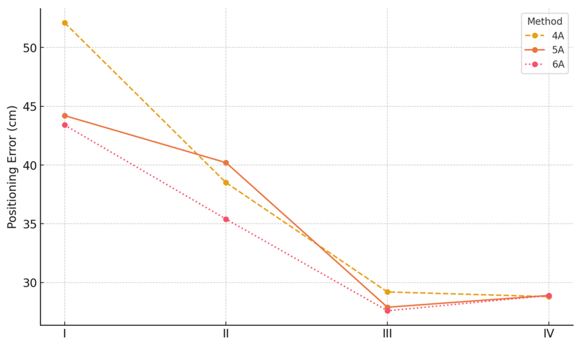
Figure 16 presents the resulting positioning error trends corresponding to the tested ${\omega }_A$ ratios. The results show a general reduction in localization error as the influence of NLOS anchors is diminished. However, a minor performance degradation is observed at configuration IV, where the mean error in the six-anchor setup increases from 27.6 cm to 28.9 cm. Based on these observations, the 9:1 weighting ratio, which yields the lowest overall error, is selected for use in subsequent experimental evaluations.

4.3. PSO Performance Evaluation Under Varying Environmental Conditions

Results from the preceding experiments indicate that the weight configuration corresponding to case III yields the most favorable localization performance. Under this setting, the average positioning error is substantially reduced, decreasing from the baseline values of 45.9 cm, 48.2 cm, and 48.2 cm to 29.2 cm, 27.9 cm, and 27.6 cm, respectively. These findings suggest that increasing the relative contribution of anchors operating under LOS conditions can effectively suppress positioning degradation in environments affected by NLOS propagation.

To further examine the robustness and adaptability of the proposed anchor-weighted PSO approach, four distinct experimental environments listed in Table 4 are incorporated into the evaluation framework. By applying the proposed method across these heterogeneous scenarios, the practical effectiveness of the weighting strategy under different propagation characteristics can be systematically assessed. The corresponding experimental outcomes are summarized below, and the weight allocations adopted for each environment are provided in

Table 12. ${\omega }_{A,Link}$ parameters in varying environmental conditions.

	4A	5A	6A
$E_1$_${\omega }_{A,LOS}$	1/4	9/40	9/40
$E_1$_${\omega }_{A,NLOS}$	0	1/10	1/20
$E_2$_${\omega }_{A,LOS}$	3/10	3/10	3/10
$E_2$_${\omega }_{A,NLOS}$	1/10	1/20	1/30
$E_3$_${\omega }_{A,LOS}$	9/20	9/20	9/20
$E_3$_${\omega }_{A,NLOS}$	1/20	1/30	1/40
$E_4$_${\omega }_{A,LOS}$	9/10	9/10	9/10
$E_4$_${\omega }_{A,NLOS}$	1/30	1/40	1/50

.

As shown in Table 12, the number of anchors operating under LOS conditions remains unchanged across the evaluated scenarios. Consequently, the assigned values of ${\omega }_{A,LOS}$ remain constant regardless of the total number of anchors involved in positioning. In the specific case of $E_1$_${\omega }_{A,LOS}$, where no anchors are affected by NLOS propagation, all four anchors operate under LOS conditions. As a result, the total weight is evenly distributed, and each anchor is assigned a weight of 0.25.

Table 13. Comparison of errors with and without PSO.

	Experiment	4A	$\mathit{P}\mathit{S}{\mathit{O}}_{4\mathit{A}}$	5A	$\mathit{P}\mathit{S}{\mathit{O}}_{5\mathit{A}}$	6A	$\mathit{P}\mathit{S}{\mathit{O}}_{6\mathit{A}}$
TP
$E_1$		13.9	10.9	32.4	17.9	34.0	16.0
$E_2$		53.9	29.2	48.2	27.9	48.2	27.6
$E_3$		62.1	56.2	60.1	54.5	52.0	50.6
$E_4$		61.7	57.9	52.7	54.6	53.6	52.1

presents a comparative analysis of localization errors across multiple environments, evaluated both with and without the proposed anchor-weighted PSO strategy. The results demonstrate that, for the majority of test scenarios, incorporating anchor weighting within the PSO framework leads to a noticeable reduction in positioning error, confirming the effectiveness of the proposed approach.

An exception is observed in the $E_1$ environment, where the positioning errors obtained with $PS{O}_{5A}$ and $PS{O}_{6A}$ slightly exceed those achieved using the conventional four-anchor configuration without weighting. This outcome indicates that when an environment already provides four anchors operating under unobstructed propagation conditions, the benefit of the proposed method becomes marginal. In such cases, the baseline four-LOS-anchor configuration already offers high localization precision, and the inclusion of additional measurements from anchors affected by NLOS propagation—despite being assigned reduced influence—introduces residual bias that can adversely affect the final position estimate.

Among the remaining experimental scenarios, the most pronounced performance improvement is observed in the $E_2$ environment. This outcome can be attributed to the presence of three anchors operating under unobstructed propagation conditions, which supply the anchor-weighted PSO algorithm with a relatively strong set of reliable range constraints. Under this configuration, the incorporation of additional NLOS-affected anchors with reduced influence enables the optimization process to compensate for the bias introduced by anchor $A_4$, thereby achieving a noticeable reduction in localization error.

By contrast, although the proposed method also provides corrective effects in the $E_3$ and $E_4$ environments, the magnitude of improvement remains limited. In these cases, the scarcity of anchors operating under LOS conditions restricts the availability of high-quality reference information, leaving the weighting mechanism with insufficient leverage to substantially mitigate NLOS-induced errors. As a result, only modest accuracy gains are realized in these more challenging scenarios.

4.4. Dynamic Simulation Analysis of Anchor-Weighted PSO

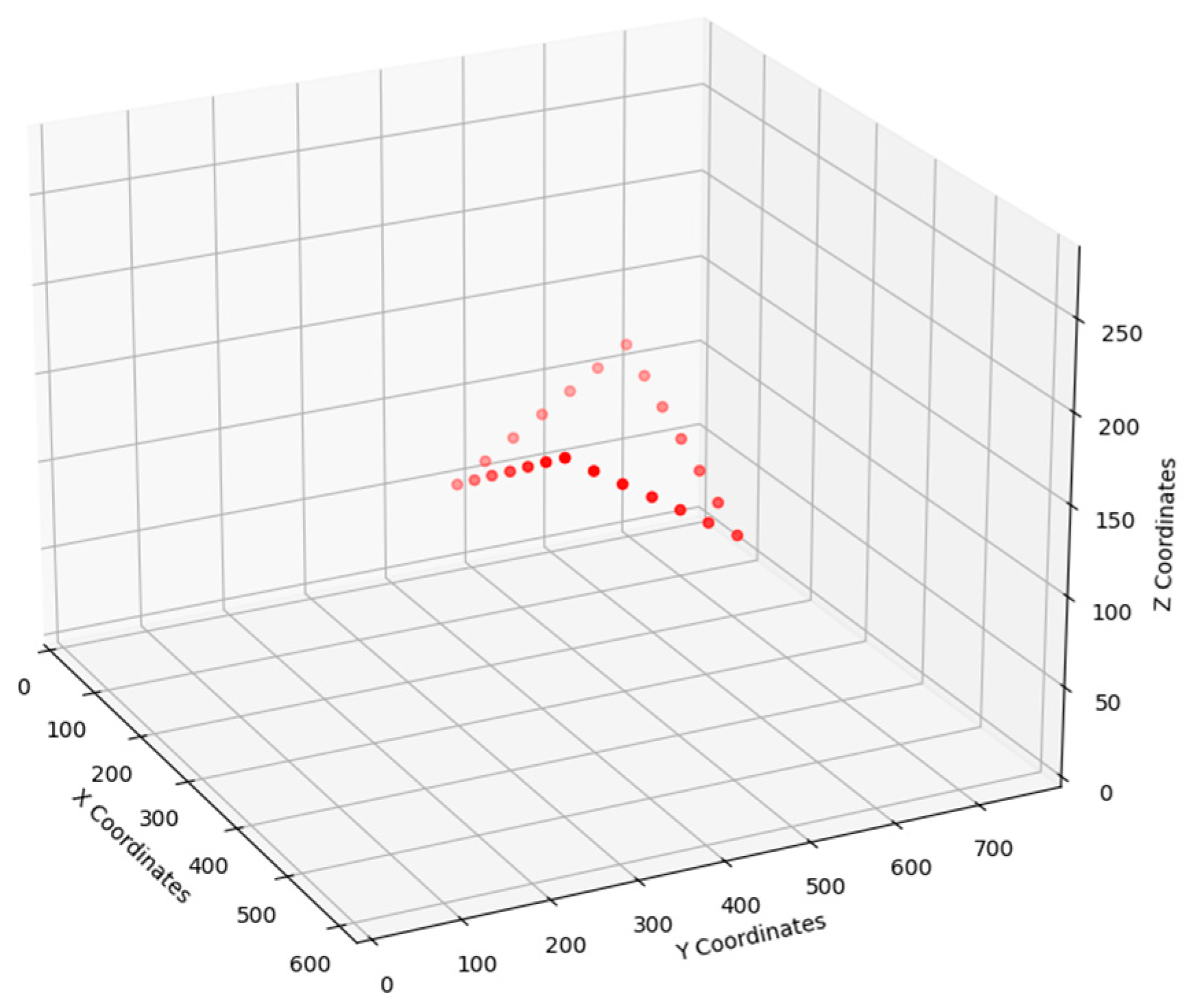
The purpose of this experiment is to assess the robustness and positioning precision of the proposed approach under conditions involving environmental variability. To this end, a trajectory consisting of 24 predefined test points (TPs) was established within the experimental area, as illustrated in Figure 17, with the corresponding spatial coordinates provided in

Table 14. Test point coordinates in dynamic simulation experiments.

	Experiment		(Unit: m) y			Experiment		(Unit: m) y
TP		x		z	TP		x		z
${\mathrm{T}\mathrm{P}}_1$		3.00	3.00	1.30	${\mathrm{T}\mathrm{P}}_{13}$		5.00	5.00	1.30
${\mathrm{T}\mathrm{P}}_2$		3.33	3.00	1.40	${\mathrm{T}\mathrm{P}}_{14}$		4.66	5.00	1.40
${\mathrm{T}\mathrm{P}}_3$		3.66	3.00	1.50	${\mathrm{T}\mathrm{P}}_{15}$		4.33	5.00	1.50
${\mathrm{T}\mathrm{P}}_4$		4.00	3.00	1.60	${\mathrm{T}\mathrm{P}}_{16}$		4.00	5.00	1.60
${\mathrm{T}\mathrm{P}}_5$		4.33	3.00	1.70	${\mathrm{T}\mathrm{P}}_{17}$		3.66	5.00	1.70
${\mathrm{T}\mathrm{P}}_6$		4.66	3.00	1.80	${\mathrm{T}\mathrm{P}}_{18}$		3.33	5.00	1.80
${\mathrm{T}\mathrm{P}}_7$		5.00	3.00	1.90	${\mathrm{T}\mathrm{P}}_{19}$		3.00	5.00	1.90
${\mathrm{T}\mathrm{P}}_8$		5.00	3.33	1.80	${\mathrm{T}\mathrm{P}}_{20}$		3.00	4.66	1.80
${\mathrm{T}\mathrm{P}}_9$		5.00	3.66	1.70	${\mathrm{T}\mathrm{P}}_{21}$		3.00	4.33	1.70
${\mathrm{T}\mathrm{P}}_{10}$		5.00	4.00	1.60	${\mathrm{T}\mathrm{P}}_{22}$		3.00	4.00	1.60
${\mathrm{T}\mathrm{P}}_{11}$		5.00	4.33	1.50	${\mathrm{T}\mathrm{P}}_{23}$		3.00	3.66	1.50
${\mathrm{T}\mathrm{P}}_{12}$		5.00	4.66	1.40	${\mathrm{T}\mathrm{P}}_{24}$		3.00	3.33	1.40

. In order to systematically evaluate the method’s behavior under differing propagation characteristics, the experimental setup was partitioned into four distinct scenarios, each defined by a different number of anchors affected by NLOS conditions. This structured design enables a detailed examination of the algorithm’s performance across a range of challenging indoor environments and facilitates an objective assessment of its applicability and reliability in real-world deployment.

Table 15. Configuration of experimental scenarios.

	LO	NL
${\mathrm{T}\mathrm{P}}_1$$\text{–}{\mathrm{T}\mathrm{P}}_6$	${\mathrm{A}}_{1-5}$	${\mathrm{A}}_6$
${\mathrm{T}\mathrm{P}}_7$$\text{–}{\mathrm{T}\mathrm{P}}_{12}$	${\mathrm{A}}_{1-4}$	${\mathrm{A}}_{5-6}$
${\mathrm{T}\mathrm{P}}_{13}$$\text{–}{\mathrm{T}\mathrm{P}}_{18}$	${\mathrm{A}}_{1-3}$	${\mathrm{A}}_{4-6}$
${\mathrm{T}\mathrm{P}}_{19}$$\text{–}{\mathrm{T}\mathrm{P}}_{24}$	${\mathrm{A}}_{1-2}$	${\mathrm{A}}_{3-6}$

summarizes the sequence of environmental transitions considered in this experiment. As the target tag progresses along the predefined path, the propagation conditions gradually become more adverse, thereby providing a basis for evaluating the corrective capability of the anchor-weighted PSO localization method. Within the table, the notation LO is used to denote the group of anchors operating under unobstructed signal conditions, whereas NL identifies those affected by NLOS propagation.

Analysis of the results presented in

Table 16. Positioning errors observed in the dynamic-environment simulation experiments.

	Experiment	4A	6A	$6{\mathit{A}}_{\mathit{P}\mathit{S}\mathit{O}}$		Experiment	4A	6A	$6{\mathit{A}}_{\mathit{P}\mathit{S}\mathit{O}}$
TP					TP
${\mathrm{T}\mathrm{P}}_1$		10.8	19.8	1.6	${\mathrm{T}\mathrm{P}}_{13}$		36.2	32.4	5.7
${\mathrm{T}\mathrm{P}}_2$		11.7	20.8	1.2	${\mathrm{T}\mathrm{P}}_{14}$		41.6	34.8	7.0
${\mathrm{T}\mathrm{P}}_3$		12.6	21.6	1.4	${\mathrm{T}\mathrm{P}}_{15}$		47.1	38.3	8.9
${\mathrm{T}\mathrm{P}}_4$		14.3	21.6	1.4	${\mathrm{T}\mathrm{P}}_{16}$		50.5	41.4	3.6
${\mathrm{T}\mathrm{P}}_5$		15.8	22.0	0.7	${\mathrm{T}\mathrm{P}}_{17}$		54.5	45.2	14.9
${\mathrm{T}\mathrm{P}}_6$		16.8	22.1	0.6	${\mathrm{T}\mathrm{P}}_{18}$		56.9	49.3	27.8
${\mathrm{T}\mathrm{P}}_7$		18.6	51.8	5.4	${\mathrm{T}\mathrm{P}}_{19}$		78.8	66.8	62.8
${\mathrm{T}\mathrm{P}}_8$		17.5	43.2	2.5	${\mathrm{T}\mathrm{P}}_{20}$		69.0	61.8	62.5
${\mathrm{T}\mathrm{P}}_9$		17.5	35.9	1.2	${\mathrm{T}\mathrm{P}}_{21}$		59.4	57.5	49.3
${\mathrm{T}\mathrm{P}}_{10}$		17.4	30.1	2.3	${\mathrm{T}\mathrm{P}}_{22}$		52.6	54.7	56.5
${\mathrm{T}\mathrm{P}}_{11}$		16.4	25.9	2.3	${\mathrm{T}\mathrm{P}}_{23}$		47.5	53.0	42.4
${\mathrm{T}\mathrm{P}}_{12}$		15.6	24.1	1.2	${\mathrm{T}\mathrm{P}}_{24}$		43.4	52.2	45.7

indicates that, for test points $T{P}_1$ through $T{P}_{12}$, the four-anchor (4A) configuration achieves exceptionally high localization precision, as each of these points is supported by at least four LOS anchors. Under this setup, the minimum observed error is as low as 1.7 cm. In contrast, when additional NLOS-affected anchors are included in the six-anchor (6A) configuration, the overall positioning accuracy decreases. Although the anchor-weighted PSO method does not produce substantial improvements in scenarios already supported by more than four LOS anchors, it generally provides modest accuracy enhancements in most cases. An exception is observed at $T{P}_7$, where the application of the weighting method unexpectedly results in a slight increase in the positioning error.

For test points $T{P}_{13}$ through $T{P}_{18}$, where NLOS propagation effects are more pronounced, the proposed method demonstrates substantial corrective capability. Notably, at $T{P}_{16}$, the localization error is dramatically reduced from 50.5 cm to 3.6 cm, indicating that the algorithm effectively compensates for the bias introduced by obstructed anchors and enhances positioning performance in challenging environments.

Finally, for $T{P}_{19}$ through $T{P}_{24}$, the number of LOS anchors is limited, restricting the influence of high-quality reference measurements. In this scenario, the anchor-weighted PSO method provides only minor reductions in positioning errors, highlighting its limitations when the majority of anchors operate under NLOS conditions. Overall, these results emphasize that the method’s effectiveness is strongly dependent on the availability of reliable LOS measurements, while still providing meaningful improvements in scenarios with mixed LOS/NLOS anchor distributions.

5. Conclusions

This study evaluated a multi-anchor UWB three-dimensional positioning system based on a PSO framework, with particular focus on the effects of LOS and NLOS propagation and the benefits of an anchor-weighted PSO strategy. Experiments were conducted across multiple anchor configurations and dynamic test points to assess positioning accuracy under varying environmental conditions.

The baseline results indicate that, with 4 to 8 anchors, positioning errors were maintained within 13.9, 10.5, 8.5, 8.8, and 12.6 cm, respectively. When all anchors operated under LOS conditions, the system achieved consistently low errors, demonstrating the high intrinsic accuracy of UWB technology. However, the presence of NLOS paths significantly increased positioning deviations, confirming the negative impact of obstructed signal paths.

Analysis of individual test points along the dynamic trajectory further illustrates the influence of LOS availability on localization performance. For test points $T{P}_1$ through $T{P}_{12}$, the four-anchor configuration already provided high precision, with a minimum error of 1.7 cm. In these cases, the anchor-weighted PSO method offered only minor improvements, except at $T{P}_7$, where it slightly increased the error. This suggests that, when sufficient LOS anchors are present, the weighting strategy has limited impact.

For $T{P}_{13}$ through $T{P}_{18}$, where NLOS propagation is more prominent, the proposed method exhibited significant corrective capability. At $T{P}_{16}$, for example, the localization error decreased sharply from 50.5 cm to 3.6 cm. This demonstrates that the anchor-weighted PSO effectively mitigates NLOS-induced distortions when combined with LOS anchors. Conversely, for $T{P}_{19}$ through $T{P}_{24}$, the scarcity of LOS anchors constrained the effectiveness of the method, resulting in only modest error reductions. These results highlight that the method’s performance is closely linked to the presence of reliable LOS measurements.

The aggregate experimental results across multiple anchor setups further support these observations. In the $E_2$ environment, leveraging low-weighted NLOS measurements alongside LOS anchors allowed the method to reduce errors by 37%, 38%, and 39% for 4, 5, and 6 anchors, respectively. In contrast, in the $E_1$ scenario, where sufficient LOS anchors were already present, the weighting method produced minimal benefit and occasionally slightly increased the positioning error. These findings emphasize that the anchor-weighted PSO approach is most effective in mixed LOS/NLOS conditions, while its impact diminishes in environments already dominated by high-quality LOS anchors.

Overall, the results confirm that UWB three-dimensional positioning exhibits high accuracy under ideal LOS conditions and that the anchor-weighted PSO method can significantly enhance performance in environments affected by NLOS propagation. The method provides a robust and practical solution for improving localization in complex indoor scenarios, particularly when NLOS anchors are present and LOS coverage is limited.

Future research plans will further improve the robustness and rigorous statistical validation of models by experimentally demonstrating PSO, GA, SSO, FA, and other evolutionary algorithms in real-time and different-scale environments.

References

- Chen, L.; Julien, O.; Lohan, E.S.; Seco-Granados, G.; Chen, R. Mobile Geospatial Computing Systems for Ubiquitous Positioning. Mob. Inf. Syst. 2018, 2018, 9138095. [Google Scholar] [CrossRef] [Scilit]
- GPS.GOV. GPS Performance & Accuracy. 2024. Available online: https://www.gps.gov/sites/default/files/2025-07/2022-GPS-SPS-performance-analysis.pdf (accessed on 15 December 2025).
- Akyildiz, I.F.; Su, W.; Sankarasubramaniam, Y.; Cayirci, E. A Survey on Sensor Networks. IEEE Commun. Mag. 2002, 40, 102–114. [Google Scholar] [CrossRef] [Scilit]
- Er Rida, M.; Liu, F.; Jadi, Y.; Algawhari, A.A.A.; Askourih, A. Indoor Location Position Based on Bluetooth Signal Strength. In Proceedings of the 2015 2nd International Conference on Information Science and Control Engineering, Shanghai, China, 24–26 April 2015; pp. 769–773. [Google Scholar]
- Xu, Y.; Gui, G.; Gacanin, H.; Adachi, F. A Survey on Resource Allocation for 5G Heterogeneous Networks: Current Research, Future Trends, and Challenges. IEEE Commun. Surv. Tutor. 2021, 23, 668–695. [Google Scholar] [CrossRef] [Scilit]
- Shafi, M.; Molisch, A.F.; Smith, P.J.; Haustein, T.; Zhu, P.; De Silva, P.; Tufvesson, F.; Benjebbour, A.; Wunder, G. 5G: A Tutorial Overview of Standards, Trials, Challenges, Deployment, and Practice. IEEE J. Sel. Areas Commun. 2017, 35, 1201–1221. [Google Scholar] [CrossRef] [Scilit]
- Huang, Y.-F.; Chen, C.-M.; Liao, J.-Y.; Chan, T.-J. An Improved Localization Method Using Light Detection and Ranging for Indoor Positionings. Electronics 2025, 14, 4904. [Google Scholar] [CrossRef] [Scilit]
- Wski, S.; Spachos, P. Wi-Fi Indoor Positioning System Based on RSSI Measurements from Wi-Fi Access Points—A Tri-lateration Approach. Int. J. Electron. Telecommun. 2016, 62, 247–252. [Google Scholar]
- Wei, Z.; Zhou, Z. A Combined Filtering Method for ZigBee Indoor Distance Measurement. Sensors 2024, 24, 3164. [Google Scholar] [CrossRef] [Scilit] [PubMed]
- Sun, W.; Yang, F. A Robust Indoor Positioning Method based on Bluetooth Low Energy with Separate Channel Information. Sensors 2019, 19, 3487. [Google Scholar] [CrossRef] [Scilit] [PubMed]
- Merenda, M.; Catarinucci, L.; Colella, R.; Iero, D.; Della Corte, F.G.; Carotenuto, R. Exploiting RFID Technology for Indoor Positioning. In Proceedings of the 2021 6th International Conference on Smart and Sustainable Technologies (SpliTech), Bol and Split, Croatia, 8–11 September 2022; pp. 1–10. [Google Scholar]
- Rossi, F.; Tomeo, S.; Bellavista, P. RFID-Based Indoor Positioning Using Edge Machine Learning. IEEE Commun. Surv. Tutor. 2023, 24, 450–465. [Google Scholar]
- Sung, S.; Kim, H.; Jung, J.-I. Accurate Indoor Positioning for UWB-based Personal Devices using Deep Learning. IEEE Access 2023, 11, 222–229. [Google Scholar] [CrossRef] [Scilit]
- De Cock, C.; Tanghe, E.; Joseph, W.; Plets, D. Robust IMU-Based Mitigation of Human Body Shadowing in UWB Indoor Positioning. Sensors 2023, 23, 8289. [Google Scholar] [CrossRef] [Scilit]
- Barral, V.; Escudero, C.J.; García-Naya, J.A.; Catoira, R.M. NLOS Identification and Mitigation Using Low-Cost UWB Devices. Sensors 2019, 19, 3464. [Google Scholar] [CrossRef] [Scilit]
- Yang, Z.; Wang, Y.; Chen, G.; Zhang, Y. Research on High Precision Indoor Positioning Technology of UWB. J. Navig. Position. 2014, 2, 31–35. [Google Scholar]
- Xu, S. Optimal Sensor Placement for Target Localization Using Hybrid RSS, AOA and TOA Measurements. IEEE Commun. Lett. 2020, 24, 1966–1970. [Google Scholar] [CrossRef] [Scilit]
- Chen, X.; Xie, Y.; Zhou, Z.; He, Y.; Wang, Q.; Chen, Z. An Indoor 3D Positioning Method Using Terrain Feature Matching for PDR Error Calibration. Electronics 2024, 13, 1468. [Google Scholar] [CrossRef] [Scilit]
- Guo, H.; Li, M.; Zhang, X.; Gao, X.; Liu, Q. UWB indoor positioning optimization algorithm based on genetic annealing and clustering analysis. Front. Neurorobotics 2022, 16, 715440. [Google Scholar] [CrossRef] [Scilit]
- Cuevas, E.; Cienfuegos, M.; Zaldívar, D.; Pérez-Cisneros, M. A swarm optimization algorithm inspired in the behavior of the social-spider. Expert Syst. Appl. 2013, 40, 6374–6384. [Google Scholar] [CrossRef] [Scilit]
- Ariyaratne, M.K.A.; Pemarathne, W.P.J. A review of recent advancements of firefly algorithm: A modern nature inspired algorithm. In Proceedings of the 8th International Research Conference; KDU: Ratmalana, Sri Lanka, 2015; pp. 61–66. [Google Scholar]
- Qiu, J.; Xie, J.; Cheng, F. A hybrid social spider opti-mization algorithm with differential evolution for globaloptimization. J. Univers. Comput. Sci. 2017, 23, 619–635. [Google Scholar]
- Chen, Y.Y.; Huang, S.P.; Wu, T.W.; Tsai, W.T.; Liou, C.Y.; Mao, S.G. UWB System for Indoor Positioning and Tracking With Arbitrary Target Orientation, Optimal Anchor Location, and Adaptive NLOS Mitigation. IEEE Trans. Veh. Technol. 2020, 69, 9304–9314. [Google Scholar] [CrossRef] [Scilit]
- Che, F.; Ahmed, Q.Z.; Lazaridis, P.I.; Sureephong, P.; Alade, T. Indoor Positioning System (IPS) Using Ultra-Wide Bandwidth (UWB)—For Industrial Internet of Things (IIoT). Sensors 2023, 23, 8360. [Google Scholar] [CrossRef] [Scilit]
- Coppens, D.; Shahid, A.; Lemey, S.; Van Herbruggen, B.; Marshall, C.; De Poorter, E. An Overview of UWB Standards and Organizations (IEEE 802.15.4, FiRa, Apple): Interoperability Aspects and Future Research Directions. IEEE Access 2022, 10, 70219–70241. [Google Scholar] [CrossRef] [Scilit]
- Decawave. DW1000 User Manual; User Manual; Decawave: Dublin, Ireland, 2017. [Google Scholar]
- Decawave. DW1000 Datasheet; Datasheet; Decawave: Dublin, Ireland, 2017. [Google Scholar]
- Laadung, T.; Ulp, S.; Alam, M.M.; Le Moullec, Y. Active-Passive Two-Way Ranging Using UWB. In Proceedings of the 2020 14th International Conference on Signal Processing and Communication Systems (ICSPCS), Adelaide, Australia, 14–16 December 2020. [Google Scholar]
- Huang, Y.-F.; Chen, G.-Y.; Wang, H.-W. PSO-Optimized Anchor Weighting for NLOS-Resilient UWB Localization in Multipath Indoor Environment. In Proceedings of the International Conference on Cloud and Network Computing, Fuzhou, China, 6–8 June 2025; pp. 200–211. [Google Scholar]
- Kennedy, J.; Eberhart, R. Particle Swarm Optimization. In Proceedings of the ICNN’95—International Conference on Neural Networks, Perth, Australia, 27 November–1 December 1995; pp. 1942–1948. [Google Scholar]
- Eberhart, R.; Kennedy, J. A New Optimizer Using Particle Swarm Theory. In Proceedings of the Sixth International Symposium on Micro Machine and Human Science, Nagoya, Japan, 4–6 October 1995; pp. 39–43. [Google Scholar]