A Numerical Approach for the Simultaneous Identification of a Source Term and a Robin Boundary Coefficient in Time-Fractional Reaction–Diffusion Equations

Abstract

In the present study, we develop numerical approaches for the simultaneous determination of a time-dependent right-hand side and a Robin boundary coefficient in linear and quasilinear Caputo time-fractional reaction–diffusion problems based on boundary and interior observations. The well-posedness of the corresponding direct problems is established. A temporal semidiscretization is first constructed using the $L2-1_{\sigma }$ scheme, and the solution is decomposed with respect to the unknown functions. The correctness of the proposed method is proved. For the nonlinear diffusion problem, a quasilinearization technique is employed, and the spatial discretization is carried out using finite difference schemes. An iterative procedure is developed to solve the resulting inverse problem. Numerical simulations with noisy data are presented and discussed to demonstrate the efficiency of the method.

1. Introduction

Inverse problems play a central role in many areas of science and engineering, as they aim to identify unknown model components from indirect or incomplete observations. Such problems are typically ill-posed in the sense of Hadamard, since the existence, uniqueness, or stability of solutions may fail, and therefore they require careful analytical and numerical treatment [1,2,3,4,5,6].

Inverse problems for reaction–diffusion equations arise naturally in applications such as thermal diagnostics, chemical kinetics, biological processes, and environmental modeling, where reaction rates, source terms, or boundary interactions must be identified from temperature or concentration measurements [7,8]. In the fractional-order setting, such inverse problems are particularly meaningful, since time-fractional diffusion models provide an accurate description of memory and anomalous transport effects, while simultaneously leading to increased ill-posedness and mathematical complexity [9,10].

Direct problems for time-fractional diffusion equations with Caputo derivatives are well studied in the literature, and well-posedness results under various structural assumptions are available. Existence and uniqueness results for linear time-fractional diffusion equations are established in [11,12,13,14], while the case of problems with Robin boundary conditions is treated in [15].

Well-posedness results for quasilinear time-fractional diffusion problems have also been obtained within the framework of evolution equations with nonlinear operators of divergence type; see, e.g., [16]. More recently, time-fractional quasilinear reaction–diffusion systems with Dirichlet and Robin (or Neumann) boundary conditions have been analyzed in [17], where the existence and uniqueness of classical solutions are proved under stronger regularity assumptions on the data and the nonlinear diffusion term.

Further abstract well-posedness results for time-fractional evolution equations with monotone and quasilinear operators can be found in [18].

Inverse problems concerned with the identification of time-dependent source terms in mainly linear parabolic partial differential equations have been widely studied, often using pointwise or integral observations.

In the classical (integer-order) setting, existence and uniqueness results for inverse problems with time-dependent sources have been established, for example, in [2,3,19,20]. Solution methods for such problems are extensively discussed in the monographs [1,5,6,21]. In addition, various numerical methods have been developed, including the boundary element method along with Tikhonov regularization [19], finite difference schemes combined with the Tikhonov regularization [22], the meshless local radial point interpolation method coupled with the finite difference method [23], the meshless local collocation method based on radial basis functions [24], the Crank-Nicolson method with an iterative procedure [20], and the loaded equation finite difference method [25].

Inverse time-dependent source problems for sub-diffusion equations have also attracted increasing attention in recent years. For instance, in [26] the existence and uniqueness of the solution of the inverse problem for a time-fractional diffusion problem with integral observations are proved, and a meshless method based on radial basis functions is employed to solve this problem. An iterative generalized quasi-boundary value regularization method is developed in [27], while two-dimensional inverse source problems with two overspecified conditions are investigated in [28]. Well-posedness of an inverse problem for the reconstruction of a time-dependent source in a two-term time-fractional heat equation with nonlocal boundary conditions and energy measurements is proved in [29]. An overview of inverse problems for fractional-order diffusion equations can be found in the review paper [30].

Inverse problems for recovering time-dependent Robin coefficients in initial-boundary value problems for classical diffusion equations from boundary measurements have been studied in [31,32,33]. Well-posedness results and a numerical method, based on a nonconforming mixed finite element approach for the inverse problem, associated with a classical two-dimensional semilinear parabolic equation under nonlocal observation are presented in [33]. A regularization method for the reconstruction of a space–time-dependent Robin coefficient is developed in [31], while a predictor-corrector method is proposed in [32] and a regularization approach is employed in [34] to determine the same time-dependent Robin coefficient on both boundaries in a one-dimensional heat conduction problem.

Related studies address the identification of the Robin coefficient in linear fractional diffusion problems with boundary overdetermination condition. In [35], the uniqueness of the inverse Robin coefficient problem is established, and a modified Newton method is employed for its numerical solution. The inverse problem of reconstructing the same Robin coefficient on both boundaries is considered in [36], where the associated variational problem is solved using a conjugate gradient method combined with Morozov’s discrepancy principle. The corresponding inverse problem for a fractional diffusion-wave equation is investigated in [37] using a hierarchical Bayesian framework with Markov random field priors and Markov chain Monte Carlo-based posterior sampling.

The recovery of a space-dependent Robin coefficient in a classical two-dimensional parabolic equation from final-time temperature measurements is studied in [38] by reformulating the problem as the minimization of a Tikhonov functional.

The simultaneous identification of multiple unknown quantities in parabolic equations has been intensively studied in recent years, including diffusion coefficients, reaction terms, source terms, and initial data; see, e.g., [39,40,41,42]. A regularization approach is employed in [43] for recovering a space–time-dependent Robin coefficient and heat flux in a classical linear parabolic system. In [44], an inverse problem for the simultaneous reconstruction of a space-dependent source term and a Robin boundary coefficient in a linear sub-diffusion equation is investigated based on boundary and interior observations. Uniqueness results are established using unique continuation arguments and a fractional Hopf lemma, and a Tikhonov regularization approach is used for the numerical recovery. However, to the best of our knowledge, solution methods for the coupled recovery of a time-dependent Robin coefficient and a source intensity factor for sub-diffusion equations, in both linear and nonlinear settings, have not been reported in the literature.

In this study, we develop a numerical method for the simultaneous identification of a time-dependent source term and a Robin boundary coefficient in linear and quasilinear time-fractional reaction–diffusion problems from boundary and interior measurements.

The remainder of the paper is organized as follows. In the next section, we formulate the inverse problem. Section 3 presents a numerical approach for the inverse problem of recovering the right-hand side and the Robin boundary coefficient in a linear Caputo time-fractional reaction–diffusion equation using additional measurements on the Robin boundary and at an interior point. In Section 4, we extend this approach to the corresponding quasilinear time-fractional reaction–diffusion problem. Numerical simulation results are presented and discussed in Section 5. Finally, concluding remarks are given in the Section 6.

2. Physical Background and Problem Formulation

We consider the following time-fractional reaction–diffusion equation:

$${\displaystyle \frac{{\partial }^{\alpha }u}{\partial t^{\alpha }}}(x,t)-{\displaystyle \frac{\partial }{\partial x}}\left(k(·){\displaystyle \frac{\partial u}{\partial x}}(x,t)\right)+b\left(x\right)u(x,t)=\tilde{f}(x,t),0<x<L,0<t<T,$$

(1)

where ${\displaystyle \frac{{\partial }^{\alpha }}{\partial t^{\alpha }}}$ is the Caputo time-fractional derivative of order $\alpha$,

$${\displaystyle \frac{{\partial }^{\alpha }u(x,t)}{\partial t^{\alpha }}}={\displaystyle \frac{1}{\Gamma (1-\alpha )}}\underset{0}{\overset{t}{\int }}{\displaystyle \frac{\partial u(x,s)}{\partial s}}{(t-s)}^{-\alpha }ds,0<\alpha <1,$$

and $\Gamma (·)$ is the Gamma function. The unknown function $u(x,t)$ denotes the temperature at the position $x\in (0,L)$ and time $t\in (0,T)$, $k(·)$ is the thermal conductivity coefficient, $b\left(x\right)\ge 0$ is the reaction (or dissipation) coefficient, and $\tilde{f}(x,t)$ represents an internal (heat) source.

In this work, we consider both linear and nonlinear versions of Equation (1),

$$k(·)=k\left(x\right)\mathrm{and}k(·)=k\left(u\right),$$

corresponding, respectively, to a spatially varying but temperature-independent conductivity and to a conductivity that depends on the local temperature. Moreover, we assume that the source term admits the separable representation

$$\tilde{f}(x,t)=\lambda \left(t\right)f(x,t),$$

where $\lambda \left(t\right)$ is a time-dependent intensity factor and $f(x,t)$ is a shape function describing the prescribed spatio-temporal distribution of the source, up to the scalar modulation $\lambda \left(t\right)$. In particular, $f(x,t)$ may encode the geometry and placement of heaters or reactive zones, while $\lambda \left(t\right)$ accounts for the overall input power or reaction rate.

Equation (1) arises in the mathematical modeling of heat conduction in one-dimensional settings, where the temperature can be effectively described by a scalar field depending on a single spatial variable; see, for example, the monograph [45]. Such fractional diffusion models have been extensively studied in the literature; see, e.g., [10] and the review paper [9].

In the linear case $k(·)=k\left(x\right)$, the coefficient reflects spatial variations in material properties, for instance due to layering, coatings, or changes in porosity [13,14]. In the nonlinear case $k(·)=k\left(u\right)$, the thermal conductivity depends on the temperature itself, which is a common feature in many applications involving high temperature gradients, phase change processes, thermally sensitive composites, or porous media with temperature-dependent saturation [11,15,46,47].

At the left boundary we consider a Robin boundary condition

$$-k(·){\displaystyle \frac{\partial u}{\partial x}}(0,t)+\beta \left(t\right)u(0,t)=r\left(t\right),0<t<T,$$

(2)

while on the right boundary $x=L$ we prescribe a Dirichlet condition

$$u(L,t)=g\left(t\right),0<t<T.$$

(3)

Here $\beta \left(t\right)$ is a time-dependent heat transfer coefficient, and $r\left(t\right)$ represents a prescribed boundary input, for instance, arising from an ambient temperature or an imposed convective heat exchange.

A recent detailed discussion of the physical meaning and modeling aspects of Robin-type conditions for heat transfer can be found in [48]. In many applications, the coefficient $\beta$ may depend on time due to changes in the flow regime, surface properties (e.g., oxidation, fouling), or external control (e.g., switching fans, varying fluid velocity); see, e.g., [36,47,49,50].

The process starts from a known initial temperature distribution

$$u(x,0)=u_0\left(x\right),0\le x\le L.$$

(4)

In the classical direct problem associated with Equations (1)–(4), all input data (initial and boundary conditions, coefficients, right-hand side, etc.) are known, and the goal is to determine the temperature field $u(x,t)$. In contrast, inverse problems aim at identifying certain components of the model, in addition to the solution itself, from additional (overspecified) observations.

In many practical applications, the time-dependent source intensity $\lambda \left(t\right)$ and the heat transfer coefficient $\beta \left(t\right)$ are not directly measurable and must be reconstructed from indirect temperature observations. This situation commonly arises in thermal diagnostics, where internal heat generation and convective boundary effects cannot be monitored in real time, while temperature measurements are available only at discrete spatial locations inside the domain or on its boundary. Such inverse settings are typical in the analysis of composite materials, battery systems, chemical reactors, and biological tissues; see, e.g., [7,8,21].

Inverse problem. Given the known data $k(·)$, $b\left(x\right)$, $f(x,t)$, $u_0\left(x\right)$, $g\left(t\right)$, $r\left(t\right)$, $\phi \left(t\right)$, $\psi \left(t\right)$, we seek the triplet $\left(u(x,t),\lambda \left(t\right),\beta \left(t\right)\right)$ in Equations (1)–(4), assuming that the temperature is measured at two points, $x_1^{*}=0$ and $x_2^{*}\in (0,L)$:

$$u(x_1^{*},t)=\phi \left(t\right),u(x_2^{*},t)=\psi \left(t\right),0<t<T,$$

(5)

where $\phi \left(t\right)$ and $\psi \left(t\right)$ denote the measured temperature profiles.

Such measurements are standard in experimental setups employing thermocouples or embedded sensors and have been extensively used in inverse source and coefficient identification problems; see, for example, [49,50].

In the separable representation of the source term, $\tilde{f}(x,t)=\lambda \left(t\right)f(x,t)$, the function $f(x,t)$ is assumed to be known, while the time-dependent factor $\lambda \left(t\right)$ is unknown. Such factorizations are commonly used in inverse source problems for parabolic and fractional diffusion equations; see, e.g., [19,20,22,23,27]. Recovering $\lambda \left(t\right)$ therefore provides quantitative information on the temporal evolution of the internal heat generation.

3. Linear Problem

In this section, we develop numerical approach for solving the inverse problem in the case $k=k\left(x\right)$.

First, we briefly discuss the well-posedness of the direct initial-boundary value problem associated with Equations (1)–(4) for given functions $\lambda \left(t\right)$ and $\beta \left(t\right)$ and $k=k\left(x\right)$.

Theorem 1.

Assume that $k\left(x\right)\in C^1\left([0,L]\right)$ with $k\left(x\right)\ge k_0>0$ for all $x\in [0,L]$, $b\left(x\right)\in L_{\infty }(0,L)$, $b\left(x\right)\ge 0$, $x\in (0,L)$, $\tilde{f}(x,t)\in L^2((0,T),L^2(0,L))$, $u_0\left(x\right)\in H^1(0,L)$, $\beta \left(t\right)\in L_{\infty }(0,T)$, $\beta \left(t\right)\ge -{\beta }_0$, ${\beta }_0\ge 0$, $r\left(t\right)\in L^2(0,T)$, and $g\left(t\right)\in H^1(0,T)$, where $g\left(t\right)$ is compatible with $u_0$ at $t=0$ in the sense that $g\left(0\right)=u_0\left(L\right)$. Then the linear initial-boundary value problem (Equations (1)–(4)) admits a unique weak solution $u(x,t)\in L^2((0,T),H^1(0,L))\cap C([0,T],L^2(0,L))$, ${\displaystyle \frac{{\partial }^{\alpha }u}{\partial t^{\alpha }}(x,t)\in L^2((0,T),H^{-1}(0,L)),}$ and this solution depends continuously on the input data.

Proof. 

Outline of the proof. The result follows from well-established theory for linear time-fractional diffusion equations with Caputo derivatives and variable coefficients; see [11,12,13,14,15].

By a standard boundary data shifting argument (see, e.g., [11,13]) inhomogeneous boundary Equation (3) is reduced to a homogeneous one by subtracting a suitable extension of $g\left(t\right)$. Since $g\in H^1(0,T)$, the transformation is admissible, and the resulting problem involves a modified right-hand side belonging to the same functional spaces.

The problem can be recast in a weak variational setting in the space $V=\{v\in H^1(0,L):v\left(L\right)=0\}$, where the spatial operator together with the Robin boundary condition is represented by the corresponding time-dependent bilinear form

$$a_t(u,v)={\int }_0^{L}k\left(x\right)u_x{v}_{x}dx+{\int }_0^{L}b\left(x\right)uvdx+\beta \left(t\right)u(0,t)v\left(0\right).$$

This form is uniformly bounded on $V\times V$ and, due to $\beta \left(t\right)\ge -{\beta }_0$, satisfies a Gårding-type inequality. This follows from a trace estimate on V combined with Young’s inequality. Consequently, the associated family of operators $A\left(t\right):V\to V^{\prime }$ fits into the abstract framework of fractional evolution equations with the Caputo time-fractional derivative.

Existence and uniqueness of a weak solution then follow from the results in [11,12,13], while the treatment of the Robin boundary condition is covered by [15]. Finally, continuous dependence of the solution on the input data follows from standard energy estimates for time-fractional diffusion equations with the Caputo derivative; see, e.g., [11,12,13].    □

3.1. Semi-Discretization in Time

We start with construction of temporal semidiscretization for Equations (1)–(4), $k=k\left(x\right)$. We consider uniform partition of the time interval $[0,T]$

$${\overline{w}}_{\tau }=\left\{t_n=n\tau ,n=0,1,\dots ,N,\tau =T/N\right\},$$

and denote by $v^{n+1}=v^{n+1}\left(x\right)$, the approximation of the function $v(x,t)$ at $(x,t_{n+1})$.

For the Caputo fractional derivative we employ the $L2-1_{\sigma }$ formula, introduced in [51]. Let $t_{n+\sigma }=(n+\sigma )\tau$, $\sigma =1-\alpha /2$, $n=0,1,\dots ,N-1$. Thus, we approximate the fractional derivative at time $t_{n+\sigma }$ as follows:

$${\displaystyle \frac{{\partial }^{\alpha }u}{\partial t^{\alpha }}}{|}_{(x_i,t_{n+\sigma })}\approx D^{\alpha }{u}^{n+\sigma }:=q_{n,0}{u}^{n+1}-\sum _{j=0}^n\left(q_{n,n-j}-q_{n,n-j+1}\right)u^j,n=0,1,\dots ,N-1.$$

(6)

Here, $u^{n+\sigma }=u(x,t_{n+\sigma })$ and we set $q_{n,n+1}:=0$, ${\displaystyle q_{0,0}=\frac{{\tau }^{-\alpha }}{\Gamma (2-\alpha )}{a}_0}$, and for $n\ge 1$

$$q_{n,j}={\displaystyle \frac{{\tau }^{-\alpha }}{\Gamma (2-\alpha )}}\left\{\begin{array}{cc}{\displaystyle a_0+b_1,}\hfill & j=0,\hfill \\ {\displaystyle a_j+b_{j+1}-b_j,}\hfill & 1\le j\le n-1,\hfill \\ {\displaystyle a_n-b_n,}\hfill & j=n,\hfill \end{array}\right.$$

where

$$\begin{array}{ccc}\hfill a_0& =& {\sigma }^{1-\alpha },\hfill \\ \hfill a_l& =& {(l+\sigma )}^{1-\alpha }-{(l-1+\sigma )}^{1-\alpha },l\ge 1,\hfill \\ \hfill b_l& =& {\displaystyle \frac{1}{2-\alpha }}\left[{(l+\sigma )}^{2-\alpha }-{(l-1+\sigma )}^{2-\alpha }\right]-{\displaystyle \frac{1}{2}}\left[{(l+\sigma )}^{1-\alpha }+{(l-1+\sigma )}^{1-\alpha }\right],l\ge 1.\hfill \end{array}$$

The parameter $\sigma$ enters the $L2-1_{\sigma }$ scheme through the coefficients $q_{n,j}$, which depend on $\sigma$ and determine the accuracy of the approximation.

Using (6), we write a temporal semidiscretization of Equations (1)–(4) for the unknown solution $u^{n+1}=u^{n+1}\left(x\right)$, $n=0,1,\dots ,N-1$

$$\begin{array}{c}{q}_{n,0}{u}^{n+1}-\sigma {\displaystyle \frac{\partial }{\partial x}}\left(k\left(x\right){\displaystyle \frac{\partial u^{n+1}}{\partial x}}\right)+\sigma b\left(x\right)u^{n+1}=\sigma \lambda \left(t^{n+1}\right)f(x,t^{n+1})\hfill \\ +(1-\sigma )\lambda \left(t^n\right)f(x,t^n)-(1-\sigma )b\left(x\right)u^n+(1-\sigma ){\displaystyle \frac{\partial }{\partial x}}\left(k\left(x\right){\displaystyle \frac{\partial u^n}{\partial x}}\right)\hfill \\ +\sum _{j=0}^n\left(q_{n,n-j}-q_{n,n-j+1}\right)u^j,0<x<L,\hfill \\ -k\left(0\right){\displaystyle \frac{\partial u^{n+1}}{\partial x}}\left(0\right)+\beta \left(t^{n+1}\right)u^{n+1}\left(0\right)=r\left(t^{n+1}\right),\hfill \\ u^{n+1}\left(L\right)=g\left(t^{n+1}\right),\hfill \\ u^0\left(x\right)=u_0\left(x\right),0\le x\le L,\hfill \end{array}$$

(7)

Next, we proceed to the solution of the inverse problem at the semidiscrete level. Taking into account that ${\beta }^{n+1}=\beta \left(t_{n+1}\right)$ is an unknown function, we linearize the Robin boundary condition in Equation (7)

$$-k\left(0\right){\displaystyle \frac{\partial u^{n+1}}{\partial x}}\left(0\right)+{\beta }^{n+1}{u}^n\left(0\right)+{\beta }^n{u}^{n+1}\left(0\right)-{\beta }^n{u}^n\left(0\right)=r\left(t^{n+1}\right).$$

(8)

Then, we consider the following decomposition of the solution:

$$u^{n+1}\left(x\right)=Y^{n+1}\left(x\right)+{\beta }^{n+1}{W}^{n+1}\left(x\right)+{\lambda }^{n+1}{Z}^{n+1}\left(x\right).$$

(9)

Substituting Equation (9) in Equation (7) with the Robin boundary condition replaced by Equation (8), we obtain the following three problems:

$$\begin{array}{c}{q}_{n,0}{Y}^{n+1}-\sigma {\displaystyle \frac{d}{dx}}\left(k\left(x\right){\displaystyle \frac{d{Y}^{n+1}}{dx}}\right)+\sigma b\left(x\right)Y^{n+1}=(1-\sigma ){\displaystyle \frac{d}{dx}}\left(k\left(x\right){\displaystyle \frac{d{u}^n}{dx}}\right)-(1-\sigma )b\left(x\right)u^n\hfill \\ +(1-\sigma )\lambda \left(t^n\right)f(x,t^n)+\sum _{j=0}^n\left(q_{n,n-j}-q_{n,n-j+1}\right)u^j,0<x<L,\hfill \\ -k\left(0\right){\displaystyle \frac{d{Y}^{n+1}}{dx}}\left(0\right)+{\beta }^n{Y}^{n+1}\left(0\right)=r\left(t^{n+1}\right)+{\beta }^n{u}^n\left(0\right),\hfill \\ Y^{n+1}\left(L\right)=g\left(t^{n+1}\right),\hfill \\ u^0\left(x\right)=u_0\left(x\right),0\le x\le L,\hfill \end{array}$$

(10)

$$\begin{array}{c}{q}_{n,0}{W}^{n+1}-\sigma {\displaystyle \frac{d}{dx}}\left(k\left(x\right){\displaystyle \frac{d{W}^{n+1}}{dx}}\right)+\sigma b\left(x\right)W^{n+1}=0,0<x<L,\hfill \\ -k\left(0\right){\displaystyle \frac{d{W}^{n+1}}{dx}}\left(0\right)+{\beta }^n{W}^{n+1}\left(0\right)=-u^n\left(0\right),\hfill \\ W^{n+1}\left(L\right)=0,\hfill \\ u^0\left(x\right)=u_0\left(x\right),0\le x\le L,\hfill \end{array}$$

(11)

$$\begin{array}{c}{q}_{n,0}{Z}^{n+1}-\sigma {\displaystyle \frac{d}{dx}}\left(k\left(x\right){\displaystyle \frac{d{Z}^{n+1}}{dx}}\right)+\sigma b\left(x\right)Z^{n+1}=\sigma f(x,t^{n+1}),0<x<L,\hfill \\ -k\left(0\right){\displaystyle \frac{d{Z}^{n+1}}{dx}}\left(0\right)+{\beta }^n{Z}^{n+1}\left(0\right)=0,\hfill \\ Z^{n+1}\left(L\right)=0.\hfill \end{array}$$

(12)

After solving Equations (10)–(12) to obtain the solutions $Y^{n+1}\left(x\right)$, $W^{n+1}\left(x\right)$ and $Z^{n+1}\left(x\right)$, $0\le x\le L$, we use the measurements of Equation (5) at $x_1^{*}$ and $x_2^{*}$ in the representation of Equation (9) to obtain

$$M^{n+1}\left(\begin{array}{c}{\beta }^{n+1}\\ {\lambda }^{n+1}\end{array}\right)=\left(\begin{array}{c}{\phi }^{n+1}-Y^{n+1}\left(x_1^{*}\right)\\ {\psi }^{n+1}-Y^{n+1}\left(x_2^{*}\right)\end{array}\right),M^{n+1}=\left(\begin{array}{cc}{W}^{n+1}\left(0\right)& Z^{n+1}\left(0\right)\\ W^{n+1}\left(x_2^{*}\right)& Z^{n+1}\left(x_2^{*}\right)\end{array}\right).$$

(13)

The solvability of the reconstruction step at time level $t_{n+1}$ is reduced to solving the $2\times 2$ linear Equation (13). Hence, this step is solvable and the pair $({\beta }^{n+1},{\lambda }^{n+1})$ is uniquely determined if $det\left(M^{n+1}\right)\ne 0$.

In general, this non-degeneracy cannot be guaranteed for arbitrary data and for an arbitrary choice of the interior measurement point $x_2^{*}$. The next lemma shows that, under a mild condition on the source term f, there always exists at least one interior point $x_2^{*}\in (0,L)$ for which $M^{n+1}$ is invertible.

Lemma 1.

Fix $n\in \{0,1,\dots ,N-1\}$ and assume that $f(·,t^{n+1})\not\equiv 0$ in $(0,L)$ and $W^{n+1}\left(0\right)\ne 0$. Then there exists at least one point $x_2^{*}\in (0,L)$ such that the matrix $M^{n+1}$ in Equation (13) is invertible, i.e., $det\left(M^{n+1}\right)\ne 0$.

Proof. 

Let

$$M^{n+1}\left(x\right)=\left(\begin{array}{cc}{W}^{n+1}\left(0\right)& Z^{n+1}\left(0\right)\\ W^{n+1}\left(x\right)& Z^{n+1}\left(x\right)\end{array}\right).$$

Define

$$G\left(x\right):=det\left(M^{n+1}\left(x\right)\right)=W^{n+1}\left(0\right)Z^{n+1}\left(x\right)-Z^{n+1}\left(0\right)W^{n+1}\left(x\right),x\in (0,L).$$

Multiplying Equation (12) by $W^{n+1}\left(0\right)$ and Equation (11) by $Z^{n+1}\left(0\right)$ and subtracting, we obtain

$$q_{n,0}G\left(x\right)-\sigma {\displaystyle \frac{d}{dx}}\left(k\left(x\right){\displaystyle \frac{dG}{dx}}\left(x\right)\right)+\sigma b\left(x\right)G\left(x\right)=W^{n+1}\left(0\right)\sigma f(x,t^{n+1}),0<x<L.$$

Assume, for contradiction, that $G\equiv 0$ on $(0,L)$. Then $G_x\equiv 0$ there as well, and hence the left-hand side of the above equation vanishes identically. Consequently, this implies

$$W^{n+1}\left(0\right)\sigma f(x,t^{n+1})\equiv 0\mathrm{in}(0,L),$$

which contradicts the assumptions $W^{n+1}\left(0\right)\ne 0$ and $f(·,t^{n+1})\not\equiv 0$. Therefore, G cannot vanish identically on $(0,L)$, and there exists at least one $x_2^{*}\in (0,L)$ with $G\left(x_2^{*}\right)\ne 0$, i.e., $det\left(M^{n+1}\right)\ne 0$ at $x_2^{*}$.    □

We now assume that the interior measurement point $x_2^{*}\in (0,L)$ has been chosen in such a way that the corresponding matrices $M^{n+1}$ are invertible for all time levels. Under this non-degeneracy assumption, we obtain the following discrete uniqueness result:

Theorem 2.

Suppose there exists a fixed point $x_2^{*}\in (0,L)$ such that for all $n=0,1,\dots ,N-1$ the matrix $M^{n+1}$ in Equation (13) is invertible. Then the semi-discrete inverse problem of determining the sequences $\left\{u^n\right\}$, $\left\{{\lambda }^n\right\}$ and $\left\{{\beta }^n\right\}$ from Equations (7)–(9), and the measurements (5) admits at most one solution.

Proof. 

Assume that $(u^n,{\lambda }^n,{\beta }^n)$ and $({\tilde{u}}^n,{\tilde{\lambda }}^n,{\tilde{\beta }}^n)$ are two solutions with the same data. Clearly $u^0={\tilde{u}}^0$. Suppose that for some $n\in \{0,1,\dots ,N-1\}$ we have $u^j={\tilde{u}}^j$, ${\beta }^j={\tilde{\beta }}^j$, ${\lambda }^j={\tilde{\lambda }}^j$ for all $j\le n$. Then the right-hand sides and coefficients of auxiliary Equations (10)–(12) coincide, and therefore $Y^{n+1}={\tilde{Y}}^{n+1}$, $W^{n+1}={\tilde{W}}^{n+1}$, $Z^{n+1}={\tilde{Z}}^{n+1}$.

Evaluating the decomposition of Equation (9) at the measurement points 0 and $x_2^{*}$ yields the linear systems

$$M^{n+1}\left(\begin{array}{c}{\beta }^{n+1}\\ {\lambda }^{n+1}\end{array}\right)=\left(\begin{array}{c}{\phi }^{n+1}-Y^{n+1}\left(0\right)\\ {\psi }^{n+1}-Y^{n+1}\left(x_2^{*}\right)\end{array}\right),M^{n+1}\left(\begin{array}{c}{\tilde{\beta }}^{n+1}\\ {\tilde{\lambda }}^{n+1}\end{array}\right)=\left(\begin{array}{c}{\phi }^{n+1}-{\tilde{Y}}^{n+1}\left(0\right)\\ {\psi }^{n+1}-{\tilde{Y}}^{n+1}\left(x_2^{*}\right)\end{array}\right).$$

Since $Y^{n+1}={\tilde{Y}}^{n+1}$ and $M^{n+1}$ is invertible, both systems have the same unique solution; hence, ${\beta }^{n+1}={\tilde{\beta }}^{n+1}$ and ${\lambda }^{n+1}={\tilde{\lambda }}^{n+1}$. Substituting these identities into Equation (9) gives $u^{n+1}={\tilde{u}}^{n+1}$. By induction, the claim holds for all n, proving uniqueness.    □

3.2. Full Discretization

Next, we introduce the spatial discretization. We define a uniform mesh on the spatial interval $[0,L]$

$${\overline{\omega }}_h=\{x_i=ih,i=0,1,\dots ,I,h=L/I\},$$

and let ${\nu }_i^n=u(x_i,t_n)$. Further, we use also the following notation:

$$K_{i+1/2}={\displaystyle \frac{k\left(x_i\right)+k\left(x_{i+1}\right)}{2}}.$$

Equations (10)–(12) are approximated using second-order finite differences, with one-sided finite difference employed for the discretization of the first derivative in the boundary conditions. The resulting numerical schemes are

$$\begin{array}{c}{\mathcal{L}}_i\left(Y^{n+1}\right):=q_{n,0}{Y}_i^{n+1}-{\displaystyle \frac{\sigma }{h^2}}\left(K_{i+1/2}(Y_{i+1}^{n+1}-Y_i^{n+1})-K_{i-1/2}(Y_i^{n+1}-Y_{i-1}^{n+1})\right)+\sigma b_i{u}_i^{n+1}\hfill \\ ={\displaystyle \frac{(1-\sigma )}{h^2}}\left(K_{i+1/2}(Y_{i+1}^{n+1}-Y_i^n)-K_{i-1/2}(Y_i^{n+1}-Y_{i-1}^n)\right)+(1-\sigma ){\lambda }^n{f}_i^n\hfill \\ -(1-\sigma )b_i{u}^n+\sum _{j=0}^n\left(q_{n,n-j}-q_{n,n-j+1}\right)u^j)u_i^j,i=1,2,\dots ,I-1,\hfill \\ {\mathcal{L}}_0\left(Y^{n+1}\right):={\displaystyle \frac{k\left(0\right)}{2h}}\left(3Y_0^{n+1}-4Y_1^{n+1}+Y_2^{n+1}\right)+{\beta }^n{Y}_0^n=r^{n+1}+{\beta }^n{u}_0^n,\hfill \\ Y_I^{n+1}=g\left(t^{n+1}\right),\hfill \\ u_i^0=u_0\left(x_i\right),i=0,1,\dots ,I,\hfill \end{array}$$

(14)

$$\begin{array}{c}{\mathcal{L}}_i\left(W^{n+1}\right)=0,0<x<L,\hfill \\ {\mathcal{L}}_0\left(W^{n+1}\right)=-u_0^n,\hfill \\ W^{n+1}\left(L\right)=0,\hfill \\ u_i^0=u_0\left(x_i\right),i=0,1,\dots ,I,\hfill \end{array}$$

(15)

$$\begin{array}{c}{\mathcal{L}}_i\left(Z^{n+1}\right)=\sigma f(x,t^{n+1}),0<x<L,\hfill \\ {\mathcal{L}}_0\left(Z^{n+1}\right)=0,\hfill \\ Z^{n+1}\left(L\right)=0.\hfill \end{array}$$

(16)

The value ${\beta }^0$ is determined exactly from initial Equation (4) and boundary Equation (2), $k=k\left(x\right)$ at the initial time as

$${\beta }^0={\displaystyle \frac{1}{u_0\left(0\right)}}\left(r^0+k\left(0\right){\displaystyle \frac{d{u}_0}{dx}}\left(0\right)\right),$$

while the value ${\lambda }^0$ is determined from initial Equation (4) and the stationary form of Equation (1) at $t=0$ as

$${\lambda }^0={\displaystyle \frac{1}{f(x_i,0)}}\left(b\left(x_i\right)u_0\left(x_i\right)-k^{\prime }\left(x_i\right){\left(u_0\left(x_i\right)\right)}^2-k\left(x_i\right){\displaystyle \frac{d^2{u}_0}{d{x}^2}}\left(x_i\right)\right),i\in \{1,2,\dots ,I-1\}.$$

Solving Equations (14)–(16), compute the auxiliary solutions $Y^{n+1}$, $W^{n+1}$, and $Z^{n+1}$. Then, using Equation (13) and together with the decomposition

$$u_i^{n+1}=Y_i^{n+1}+{\beta }^{n+1}{W}_i^{n+1}+{\lambda }^{n+1}{Z}_i^{n+1},$$

(17)

we determine ${\beta }^{n+1}$, ${\lambda }^{n+1}$, and  subsequently $u^{n+1}$.

4. Nonlinear Problem

In the nonlinear setting, we replace the spatially dependent conductivity $k\left(x\right)$ in Equation (1) and the Robin boundary condition (Equation (2)) by a temperature-dependent coefficient $k\left(u\right)$.

Under suitable assumptions on $k\left(u\right)$, we formulate the following well-posedness result.

Theorem 3.

Assume that the data $b\left(x\right)$, $\tilde{f}(x,t)$, $g\left(t\right)$, $r\left(t\right)$, $\beta \left(t\right)$, and $u_0\left(x\right)$ satisfy the conditions of Theorem 1. Let $k\left(s\right)\in C^1\left(\mathbb{R}\right)$ be such that $0<k_0\le k\left(s\right)\le k_1<\infty$, $s\in \mathbb{R}$. Then, from the nonlinear initial-boundary value Equations (1)–(4), $k=k\left(u\right)$ admits a unique weak solution $u(x,t)\in L^2((0,T),H^1(0,L))\cap C([0,T],L^2(0,L))$, ${\displaystyle \frac{{\partial }^{\alpha }u}{\partial t^{\alpha }}(x,t)\in L^2((0,T),H^{-1}(0,L)),}$ and this solution depends continuously on the input data.

Under the assumptions of Theorem 3, nonlinear Equations (1)–(4) with $k=k\left(u\right)$ fit into the general framework of quasilinear subdiffusion equations with the Caputo time-fractional derivative and monotone spatial operators.

Existence and uniqueness results for quasilinear time-fractional diffusion equations of divergence type with the Caputo derivative have been established using variational and monotonicity methods. In particular, global well-posedness for such problems under structural assumptions on the nonlinear diffusion coefficient, including those imposed on $k\left(u\right)$ in Theorem 3, is proved in [16]. Related well-posedness results for nonlinear diffusion equations with time-fractional derivatives, including uniqueness and continuous dependence properties, can also be found in [52].

Further results for time-fractional quasilinear reaction–diffusion systems with Dirichlet and Robin (or Neumann) boundary conditions, as well as for more abstract evolution equations involving monotone and quasilinear operators, are reported in [17,18]. Therefore, Theorem 3 follows as a direct consequence of these general results.

4.1. Temporal Semidiscretization

As in the linear case, we start with a semidiscretization in time.

In order to prepare the problem for decomposition of the solution, we apply the Bellman-Kalaba quasilinearization [53,54] to the nonlinear diffusion term. Assume that ${\tilde{u}}^{n+1}$ and ${\tilde{v}}^{n+1}$ are initial approximations to the corresponding exact values of $u^{n+1}$ and ${\displaystyle \frac{\partial u^{n+1}}{\partial x}}$ at the time level $t_{n+1}$, and that ${\displaystyle k^{\prime }\left(u\right)=\frac{dk}{du}}$. Thus, we obtain

$$k\left(u^{n+1}\right){\displaystyle \frac{\partial u^{n+1}}{\partial x}}\approx k\left({\tilde{u}}^{n+1}\right){\displaystyle \frac{\partial u^{n+1}}{\partial x}}+k^{\prime }\left({\tilde{u}}^{n+1}\right){\tilde{v}}^{n+1}{u}^{n+1}-k^{\prime }\left({\tilde{u}}^{n+1}\right){\tilde{u}}^{n+1}{\tilde{v}}^{n+1}.$$

(18)

Using Equation (18) and linearization for $\beta \left(t\right)u$ as in the linear case, we obtain the following semidiscrete problem:

$$\begin{array}{c}{q}_{n,0}{u}^{n+1}-\sigma {\displaystyle \frac{\partial }{\partial x}}\left(k\left({\tilde{u}}^{n+1}\right){\displaystyle \frac{\partial u^{n+1}}{\partial x}}+k^{\prime }\left({\tilde{u}}^{n+1}\right){\tilde{v}}^{n+1}{u}^{n+1}-k^{\prime }\left({\tilde{u}}^{n+1}\right){\tilde{u}}^{n+1}{\tilde{v}}^{n+1}\right)\hfill \\ +\sigma b\left(x\right)u^{n+1}=\sigma {\lambda }^{n+1}{f}^{n+1}\left(x\right)+(1-\sigma ){\lambda }^n{f}^n\left(x\right)-(1-\sigma )b\left(x\right)u^n\hfill \\ +(1-\sigma ){\displaystyle \frac{\partial }{\partial x}}\left(k\left(u^n\right){\displaystyle \frac{\partial u^n}{\partial x}}\right)+\sum _{j=0}^n\left(q_{n,n-j}-q_{n,n-j+1}\right)u^j,0<x<L,\hfill \\ -k\left({\tilde{u}}^{n+1}\left(0\right)\right){\displaystyle \frac{\partial u^{n+1}\left(0\right)}{\partial x}}-k^{\prime }\left({\tilde{u}}^{n+1}\left(0\right)\right){\tilde{v}}^{n+1}\left(0\right)u^{n+1}\left(0\right)+{\beta }^n{u}^{n+1}\left(0\right)\hfill \\ =-k^{\prime }\left({\tilde{u}}^{n+1}\left(0\right)\right){\tilde{u}}^{n+1}\left(0\right){\tilde{v}}^{n+1}\left(0\right)+r^{n+1}-{\beta }^{n+1}\left(u^n\left(0\right)-u^n\left(0\right)\right),\hfill \\ u^{n+1}\left(L\right)=g^{n+1},\hfill \\ u^0\left(x\right)=u_0\left(x\right),0\le x\le L,\hfill \end{array}$$

(19)

Applying decomposition Equation (9), Equation (19) can be reformulated as the following three auxiliary problems:

$$\begin{array}{c}{L}_i^{\mathrm{n}\mathrm{o}\mathrm{n}\mathrm{l}}\left(Y^{n+1}\right):=q_{n,0}{Y}^{n+1}-\sigma {\displaystyle \frac{\partial }{\partial x}}\left(k\left({\tilde{u}}^{n+1}\right){\displaystyle \frac{\partial Y^{n+1}}{\partial x}}+k^{\prime }\left({\tilde{u}}^{n+1}\right){\tilde{v}}^{n+1}{Y}^{n+1}\right)+\sigma b\left(x\right)Y^{n+1}\hfill \\ =-\sigma {\displaystyle \frac{\partial }{\partial x}}\left(k^{\prime }\left({\tilde{u}}^{n+1}\right){\tilde{u}}^{n+1}{\tilde{v}}^{n+1}\right)+(1-\sigma ){\lambda }^n{f}^n\left(x\right)-(1-\sigma )b\left(x\right)u^n\hfill \\ +(1-\sigma ){\displaystyle \frac{\partial }{\partial x}}\left(k\left(u^n\right){\displaystyle \frac{\partial u^n}{\partial x}}\right)+\sum _{j=0}^n\left(q_{n,n-j}-q_{n,n-j+1}\right)u^j,0<x<L,\hfill \\ L_0^{\mathrm{n}\mathrm{o}\mathrm{n}\mathrm{l}}\left(Y^{n+1}\right):=-k\left({\tilde{u}}^{n+1}\left(0\right)\right){\displaystyle \frac{\partial Y^{n+1}\left(0\right)}{\partial x}}-k^{\prime }\left({\tilde{u}}^{n+1}\left(0\right)\right){\tilde{v}}^{n+1}\left(0\right)Y^{n+1}\left(0\right)+{\beta }^n{Y}^{n+1}\left(0\right)\hfill \\ =-k^{\prime }\left({\tilde{u}}^{n+1}\left(0\right)\right){\tilde{u}}^{n+1}\left(0\right){\tilde{v}}^{n+1}\left(0\right)+r^{n+1}+{\beta }^n{u}^n\left(0\right),\hfill \\ Y^{n+1}\left(L\right)=g\left(t^{n+1}\right),\hfill \\ u^0\left(x\right)=u_0\left(x\right),0\le x\le L,\hfill \end{array}$$

(20)

$$\begin{array}{c}{L}_i^{\mathrm{n}\mathrm{o}\mathrm{n}\mathrm{l}}\left(W^{n+1}\right)=0,0<x<L,\hfill \\ L_0^{\mathrm{n}\mathrm{o}\mathrm{n}\mathrm{l}}\left(W^{n+1}\right)=-u^n\left(0\right),\hfill \\ W^{n+1}\left(L\right)=0,\hfill \\ u^0\left(x\right)=u_0\left(x\right),0\le x\le L,\hfill \end{array}$$

(21)

$$\begin{array}{c}{L}_i^{\mathrm{n}\mathrm{o}\mathrm{n}\mathrm{l}}\left(Z^{n+1}\right)=\sigma f^{n+1}\left(x\right),0<x<L,\hfill \\ L_0^{\mathrm{n}\mathrm{o}\mathrm{n}\mathrm{l}}\left(Z^{n+1}\right)=0,\hfill \\ Z^{n+1}\left(L\right)=0.\hfill \end{array}$$

(22)

After computing the solutions $Y^{n+1}$, $W^{n+1}$, and $Z^{n+1}$, $n=1,2,\dots ,N$, we use the measurement data of Equation (5) to determine ${\lambda }^{n+1}$, and ${\beta }^{n+1}$ via Equation (13), and then apply Equation (9) to obtain $u^{n+1}\left(x\right)$.

The operators $L_i^{\mathrm{n}\mathrm{o}\mathrm{n}\mathrm{l}}$ and $L_0^{\mathrm{n}\mathrm{o}\mathrm{n}\mathrm{l}}$ define a linear boundary value problem in x, since at each time level $t_{n+1}$ the coefficients $k\left({\tilde{u}}^{n+1}\right)$ and $k^{\prime }\left({\tilde{u}}^{n+1}\right){\tilde{v}}^{n+1}$ are regarded as known. Therefore, for fixed linearization data $({\tilde{u}}^{n+1},{\tilde{v}}^{n+1})$, auxiliary Equations (20)–(22) have the same structure as in the linear case.

As in the linear setting, the reconstruction of $({\beta }^{n+1},{\lambda }^{n+1})$ from the measurements of Equation (5) leads to the solution of linear Equation (13). Hence, the solvability and uniqueness of the reconstruction step depend on the invertibility of the matrix $M^{n+1}$. Consequently, the arguments of Lemma 1 and Theorem 2 can be applied to the present linearized nonlinear setting.

4.2. Full Discretization

In this section, we derive the spatial discretization of Equations (20)–(22) using second-order finite difference approximations. Using the notations

$$\begin{array}{cc}& {\displaystyle {\tilde{U}}_{i+1/2}=\frac{{\tilde{u}}_i^{n+1}+{\tilde{u}}_{i+1}^{n+1}}{2},{\overline{U}}_{i+1/2}=\frac{{\tilde{u}}_{i+1}^{n+1}-{\tilde{u}}_i^{n+1}}{h},{\overline{U}}_i^{+}=\frac{3{\tilde{u}}_0^{n+1}-4{\tilde{u}}_1^{n+1}+{\tilde{u}}_2^{n+1}}{2h},}\\ & {\displaystyle K_{i+1/2}^n=\frac{k\left(u_i^n\right)+k\left(u_{i+1}^n\right)}{2},{\tilde{K}}_{i+1/2}=\frac{k\left({\tilde{u}}_i^{n+1}\right)+k\left({\tilde{u}}_{i+1}^{n+1}\right)}{2},{\tilde{K}}_{i+1/2}^{\prime }=\frac{k^{\prime }\left({\tilde{u}}_i^{n+1}\right)+k^{\prime }\left({\tilde{u}}_{i+1}^{n+1}\right)}{2},}\end{array}$$

we obtain discrete Equations (20)–(22) as follows:

$$\begin{array}{c}{\mathcal{L}}_i^{\mathrm{n}\mathrm{o}\mathrm{n}\mathrm{l}}\left(Y^{n+1}\right):=q_{n,0}{Y}_i^{n+1}-{\displaystyle \frac{\sigma }{h}}\left({\tilde{K}}_{i+1/2}{\displaystyle \frac{Y_{i+1}^{n+1}-Y_i^{n+1}}{h}}+{\tilde{K}}_{i+1/2}^{\prime }{\overline{U}}_{i+1/2}{\displaystyle \frac{Y_{i+1}^{n+1}+Y_{i+1}^{n+1}}{2}}\right.\hfill \\ \left.-{\tilde{K}}_{i-1/2}{\displaystyle \frac{Y_i^{n+1}-Y_{i-1}^{n+1}}{h}}-{\tilde{K}}_{i-1/2}^{\prime }{\overline{U}}_{i-1/2}{\displaystyle \frac{Y_i^{n+1}+Y_{i-1}^{n+1}}{2}}\right)+\sigma b_i{Y}_i^{n+1}\hfill \\ =-{\displaystyle \frac{\sigma }{h}}\left({\tilde{K}}_{i+1/2}^{\prime }{\tilde{U}}_{i+1/2}^{n+1}{\overline{U}}_{i+1/2}-{\tilde{K}}_{i-1/2}^{\prime }{\tilde{U}}_{i-1/2}^{n+1}{\overline{U}}_{i-1/2}\right)-(1-\sigma )b_i{u}_i^n\hfill \\ +(1-\sigma ){\lambda }^n{f}_i^n+{\displaystyle \frac{1-\sigma }{h}}\left(K_{i+1/2}^n{\displaystyle \frac{u_{i+1}^n-u_i^n}{h}}-K_{i-1/2}^n{\displaystyle \frac{u_i^n-u_{i-1}^n}{h}}\right)\hfill \\ +\sum _{j=0}^n\left(q_{n,n-j}-q_{n,n-j+1}\right)u_i^j,i=1,2,\dots ,I-1,\hfill \\ {\mathcal{L}}_0^{\mathrm{n}\mathrm{o}\mathrm{n}\mathrm{l}}\left(Y^{n+1}\right):=k\left({\tilde{u}}_0^{n+1}\right){\displaystyle \frac{3Y_0^{n+1}-4Y_1^{n+1}+Y_2^{n+1}}{2h}}+k^{\prime }\left({\tilde{u}}_0^{n+1}\right){\overline{U}}_i^{+}{Y}_0^{n+1}+{\beta }^n{Y}_0^{n+1}\hfill \\ ={\beta }^n{u}_0^n+k^{\prime }\left({\tilde{u}}_0^{n+1}\right){\overline{U}}_0^{+}{\tilde{u}}_0^{n+1}+r^{n+1},\hfill \\ Y^{n+1}\left(L\right)=g^{n+1},\hfill \\ u^0\left(x\right)=u_0\left(x\right),0\le x\le L,\hfill \end{array}$$

(23)

$$\begin{array}{c}{\mathcal{L}}_i^{\mathrm{n}\mathrm{o}\mathrm{n}\mathrm{l}}\left(W^{n+1}\right)=0,i=1,2,\dots ,I-1,\hfill \\ {\mathcal{L}}_0^{nonl}\left(Y^{n+1}\right)=-u_0^n,\hfill \\ W^{n+1}\left(L\right)=0,\hfill \\ u^0\left(x\right)=u_0\left(x\right),i=1,2,\dots ,I-1,\hfill \end{array}$$

(24)

$$\begin{array}{c}{\mathcal{L}}_i^{\mathrm{n}\mathrm{o}\mathrm{n}\mathrm{l}}\left(Z^{n+1}\right)=\sigma f_i^{n+1},i=1,2,\dots ,I-1,\hfill \\ {\mathcal{L}}_0^{\mathrm{n}\mathrm{o}\mathrm{n}\mathrm{l}}\left(Y^{n+1}\right)=0,\hfill \\ Z^{n+1}\left(L\right)=0.\hfill \end{array}$$

(25)

As in the linear problem, we use Equation (5) to determine ${\beta }^{n+1}$ and ${\lambda }^{n+1}$, $n=1,2,\dots ,N$, via Equation (13), and then apply Equation (17) to obtain $u_i^{n+1}$, $i=0,1,\dots ,I-1$.

The initial values ${\beta }^0$ and ${\lambda }^0$ are determined from initial Equation (4), Robin boundary Equation (2), $k=k\left(u\right)$, and the stationary form of Equation (1), $k=k\left(u\right)$ at initial time $t=0$ as

$$\begin{array}{c}{\beta }^0={\displaystyle \frac{1}{u_0\left(0\right)}}\left(r^0+k\left(u_0\left(0\right)\right){\displaystyle \frac{d{u}_0}{dx}}\left(0\right)\right),\hfill \\ {\lambda }^0={\displaystyle \frac{1}{f(x_i,0)}}\left(b\left(x_i\right)u_0\left(x_i\right)-{\displaystyle \frac{d}{dx}}{\left(k\left(u_0\left(x\right)\right){\displaystyle \frac{d{u}_0}{dx}}\left(x\right)\right)}_{x=x_i}\right),i\in \{1,2,\dots ,I-1\}.\hfill \end{array}$$

The numerical method is implemented through an iteration procedure. Let ${\tilde{u}}_i^{n+1}$ denote the solution at the m-th iteration and time level $t_{n+1}$. The iterative process is continued until the prescribed accuracy $ϵ$ is achieved, measured in the maximum norm. The computational approach is summarized in Algorithm 1.

Algorithm 1 Numerical identification of the functions $\beta \left(t\right)$, $\lambda \left(t\right)$, and $u(x,t)$

Require: $k\left(u\right)$, $b\left(x\right)$, $f(x,t)$, $r\left(t\right)$, $u_0\left(x\right)$, $g\left(t\right)$, $\phi \left(t\right)$, $\psi \left(t\right)$, $\psi \left(t\right)$ Ensure: ${\beta }^n$, ${\lambda }^n$, $u_i^n$, $i=1,2,\dots ,I-1$, $n=1,2,\dots ,N$ Set: ${\beta }^0$ and ${\lambda }^0$, $u^{\left(0\right)}\leftarrow {\tilde{u}}^1\leftarrow u^0$ accuracy $0<ϵ<<1$ and $\delta \left(m\right)\leftarrow 1$, $m\leftarrow 0$     for  n=0:N-1 do           while $\delta \left(m\right)>ϵ$ do                 $m\leftarrow m+1$           Solve the problems (23)–(25) to find $(Y,W,Z)$ at iteration m at time $t_{n+1}$           Determine $\beta$, $\lambda$ at iteration m at time $t_{n+1}$ from (13)           Find $u^{n+1}=u^{\left(m\right)}$ from (17), using $(\beta ,\lambda ,Y,W,Z)$ at iteration m and set ${\tilde{u}}^{n+1}\leftarrow u^{\left(m\right)}$.                 $\delta \left(m\right)\leftarrow \underset{0\le i\le I}{max}|u^{\left(m\right)}-u^{(m-1)}|$           end while            return $u^{n+1}$, ${\beta }^{n+1}$, ${\lambda }^{n+1}$           $u^{\left(0\right)}\leftarrow u^{n+1}$, ${\beta }^{\left(0\right)}\leftarrow {\beta }^{n+1}$, ${\lambda }^{\left(0\right)}\leftarrow {\lambda }^{n+1}$ end for

5. Numerical Simulations

In this section, we illustrate the computational efficiency of the proposed approach for both linear and quasilinear problems.

The errors are estimated as follows:

$$\begin{array}{cc}& {\displaystyle e_{\lambda }\left(t_n\right)=\lambda \left(t_n\right)-{\lambda }^n,e_{\beta }\left(t_n\right)=\beta \left(t_n\right)-{\beta }^n,E(x_i,t_n)=u(x_i,t_n)-U_i^n,}\\ & {\displaystyle \epsilon \left(\lambda \right)=\parallel e_{\lambda }{\parallel }_2,\epsilon \left(\beta \right)=\parallel e_{\beta }{\parallel }_2,\mathcal{E}\left(u\right)=\parallel E\parallel ,}\\ & {\displaystyle {\epsilon }_r\left(\lambda \right)=\parallel e_{\lambda }{\parallel }_2/{\parallel \lambda \parallel }_2,{\epsilon }_r\left(\beta \right)=\parallel e_{\beta }{\parallel }_2/{\parallel \beta \parallel }_2,{\mathcal{E}}_r\left(u\right)=\parallel E\parallel /\parallel u\parallel ,\mathrm{where}}\\ & {\displaystyle {\parallel \nu \parallel }_2=\sqrt{\sum _{n=0}^N\tau {\left(\nu \left(t_n\right)\right)}^2},\parallel \nu \parallel =\underset{0\le i\le I}{max}\underset{0\le n\le N}{max}\left|\nu (x_i,t_n)\right|.}\end{array}$$

Noisy measurements ${\phi }^{\delta }$, ${\psi }^{\delta }$ are generated by adding perturbations to the exact data

$$\begin{array}{c}{\phi }^{\delta }\left(t_n\right)=\phi \left(t_n\right)+2\phi \left(t_n\right){\delta }_{\phi }\left({\sigma }_{\phi }\left(t\right)-0.5\right),\hfill \\ {\psi }^{\delta }\left(t_n\right)=\psi \left(t_n\right)+2\psi \left(t_n\right){\delta }_{\psi }\left({\sigma }_{\psi }\left(t\right)-0.5\right),\hfill \end{array}$$

where ${\delta }_{\phi }$, ${\delta }_{\psi }$ are noise levels and ${\sigma }_{\phi }\left(t\right)$, ${\sigma }_{\psi }\left(t\right)$ are random functions, uniformly distributed on the interval $[0,1]$. We use also the notation $\delta ={\delta }_{\phi }={\delta }_{\psi }$.

The simulations are performed for $T=1$, $L=1$, $ϵ=1.e-8$.

Example 1 (Convergence: noisy-free data). 

We illustrate the order of convergence of Algorithm 1 for exact data. Let $b=1$, $k\left(u\right)=u^4+3u$, $\beta \left(t\right)=t^4+3$, $\lambda \left(t\right)=t^3+1$, and ${\displaystyle u(x,t)=(t^3+5)cos\frac{\pi x}{4}}$. The remaining input data in Equations (1)–(3) are chosen consistently with the exact solution, and the interior measurement point is set to $x_2^{*}=0.5$. Noise-free measurements are considered, i.e., ${\delta }_{\phi }={\delta }_{\psi }=0$.

In

Table 1. Errors, convergence rates, and average number of iterations, $N=I$; Example 1.

$\mathit{\alpha }$	N	$\mathit{\epsilon }\left(\mathit{\beta }\right)$	$\mathit{CR}$	$\mathit{\epsilon }\left(\mathit{\lambda }\right)$	$\mathit{CR}$	$\mathcal{E}\left(\mathit{u}\right)$	$\mathit{CR}$	${\mathit{m}}_{\mathit{a}}$
	50	5.6001 $\times {10}^{-2}$		3.8788 $\times {10}^{-4}$		8.8976 $\times {10}^{-5}$		2.900
	100	1.3998 $\times {10}^{-2}$	2.0002	9.6415 $\times {10}^{-5}$	2.0083	2.2286 $\times {10}^{-5}$	1.9973	2.670
0.25	200	3.4989 $\times {10}^{-3}$	2.0003	2.4035 $\times {10}^{-5}$	2.0041	5.5716 $\times {10}^{-6}$	1.9999	2.610
	400	8.7464 $\times {10}^{-4}$	2.0002	6.0002 $\times {10}^{-6}$	2.0021	1.3929 $\times {10}^{-6}$	2.0000	2.468
	800	2.1865 $\times {10}^{-4}$	2.0000	1.4990 $\times {10}^{-6}$	2.0010	3.4822 $\times {10}^{-7}$	2.0000	2.210
	50	5.6106 $\times {10}^{-2}$		3.8841 $\times {10}^{-4}$		9.5363 $\times {10}^{-5}$		2.920
	100	1.4009 $\times {10}^{-2}$	2.0018	9.6450 $\times {10}^{-5}$	2.0097	2.3882 $\times {10}^{-5}$	1.9975	2.670
0.5	200	3.4998 $\times {10}^{-3}$	2.0010	2.4031 $\times {10}^{-5}$	2.0049	5.9674 $\times {10}^{-6}$	2.0007	2.610
	400	8.7463 $\times {10}^{-4}$	2.0006	5.9976 $\times {10}^{-6}$	2.0024	1.4907 $\times {10}^{-6}$	2.0011	2.468
	800	2.1862 $\times {10}^{-4}$	2.0003	1.4982 $\times {10}^{-6}$	2.0011	3.7230 $\times {10}^{-7}$	2.0015	2.210
	50	5.6321 $\times {10}^{-2}$		3.8969 $\times {10}^{-4}$		1.1419 $\times {10}^{-4}$		2.960
	100	1.4034 $\times {10}^{-2}$	2.0047	9.6580 $\times {10}^{-5}$	2.0125	2.8550 $\times {10}^{-5}$	1.9998	2.670
0.75	200	3.5025 $\times {10}^{-3}$	2.0025	2.4039 $\times {10}^{-5}$	2.0063	7.1140 $\times {10}^{-6}$	2.0048	2.610
	400	8.7484 $\times {10}^{-4}$	2.0013	5.9966 $\times {10}^{-6}$	2.0031	1.7686 $\times {10}^{-6}$	2.0081	2.468
	800	2.1861 $\times {10}^{-4}$	2.0006	1.4976 $\times {10}^{-6}$	2.0015	4.3803 $\times {10}^{-7}$	2.0135	2.210

, we present the reconstruction errors, the corresponding orders of convergence ($CR$), computed as ${log}_2$ of the ratio of errors on two consecutively refined meshes, and the average number of iterations $m_a$, for different fractional orders $\alpha$, with $I=N$.

Since the ratio $\tau =h$ is fixed for all runs, the order of convergence in space and time is estimated simultaneously. The results reported in Table 1 indicate that, for the considered test example, Algorithm 1 achieves an accuracy of $O({\tau }^2+h^2)$, and only a small number of iterations is required to attain convergence.

Further, the proposed method is examined for noisy data, nonsmooth or discontinuous functions, and weakly singular solutions.

Example 2 (Comparison: linear problem). 

We consider the linear case of Equations (1)–(3) with $k=k\left(x\right)$. Our results are compared with those reported in [35], where the inverse problem of identifying $(\beta ,u)$ in Equations (1)–(3) with $k=k\left(x\right)$ is investigated using measurements on the Robin boundary. In addition, we compare our results with the study in [36], which numerically addresses an inverse problem for determining $(\beta ,u)$ in a similar setting, but with the coefficient β appearing in Robin boundary conditions on both boundaries under boundary overspecification.

First, we reproduce the experiment whose results are reported in Table 1 of [35]. Let $k\left(x\right)=1$, $\beta \left(t\right)=1.5+sin\left(4\pi t\right)$, $b=2$, ${\displaystyle u(x,t)=t^{\alpha }+\Gamma (1+\alpha )\frac{x^2}{2}+1}$, and $\lambda \left(t\right)=e^{-t}$. All other input data are chosen consistently with the exact solution, and  $x_2^{*}=0.8$. In this case, $\phi \left(t\right)=1+t^{\alpha }$ and $\psi \left(t\right)=1+t^{\alpha }+0.32\Gamma (1+\alpha )$. The simulations are performed with $I=N=400$.

Table 2. Errors for different fractional order, $\delta =0.005$; Example 2.

$\mathit{\alpha }$	0.05	0.1	0.3	0.7	0.9	0.95
$\epsilon \left(\beta \right)$	0.0233	0.0235	0.0254	0.0531	0.1135	0.1428
${\epsilon }_r\left(\beta \right)$	0.0093	0.0094	0.0102	0.0212	0.0454	0.0571
$\mathcal{E}\left(u\right)$	0.0181	0.0176	0.0159	0.0130	0.0120	0.0124
${\mathcal{E}}_r\left(u\right)$	0.0074	0.0072	0.0065	0.0053	0.0049	0.0051

presents numerical results for different fractional orders using $\delta =0.005$. The obtained results are more sensitive to the fractional order but remain comparable to those reported in [35]. For $\alpha >0.7$, the accuracy is slightly lower compared to [35]. This behavior is expected, since in our study we simultaneously identify $(\beta ,\lambda ,u)$, whereas [35] addresses $(\beta ,u)$. The quantitative comparison with [35] shows that the errors are of the same order of magnitude, despite the increased complexity of the present inverse problem.

Next, following Example 3 in [35], we consider

$$\beta \left(t\right)=\left\{\begin{array}{cc}0,\hfill & {\displaystyle 0<t\le \frac{1}{3},}\hfill \\ 1,\hfill & {\displaystyle \frac{1}{3}<t<\frac{2}{3},}\hfill \\ 0,\hfill & {\displaystyle \frac{2}{3}\le t\le 1.}\hfill \end{array}\right.$$

The function $r\left(t\right)$ is then defined as the residual term in the Robin boundary condition, computed consistently with the exact solution and the prescribed function $\beta \left(t\right)$.

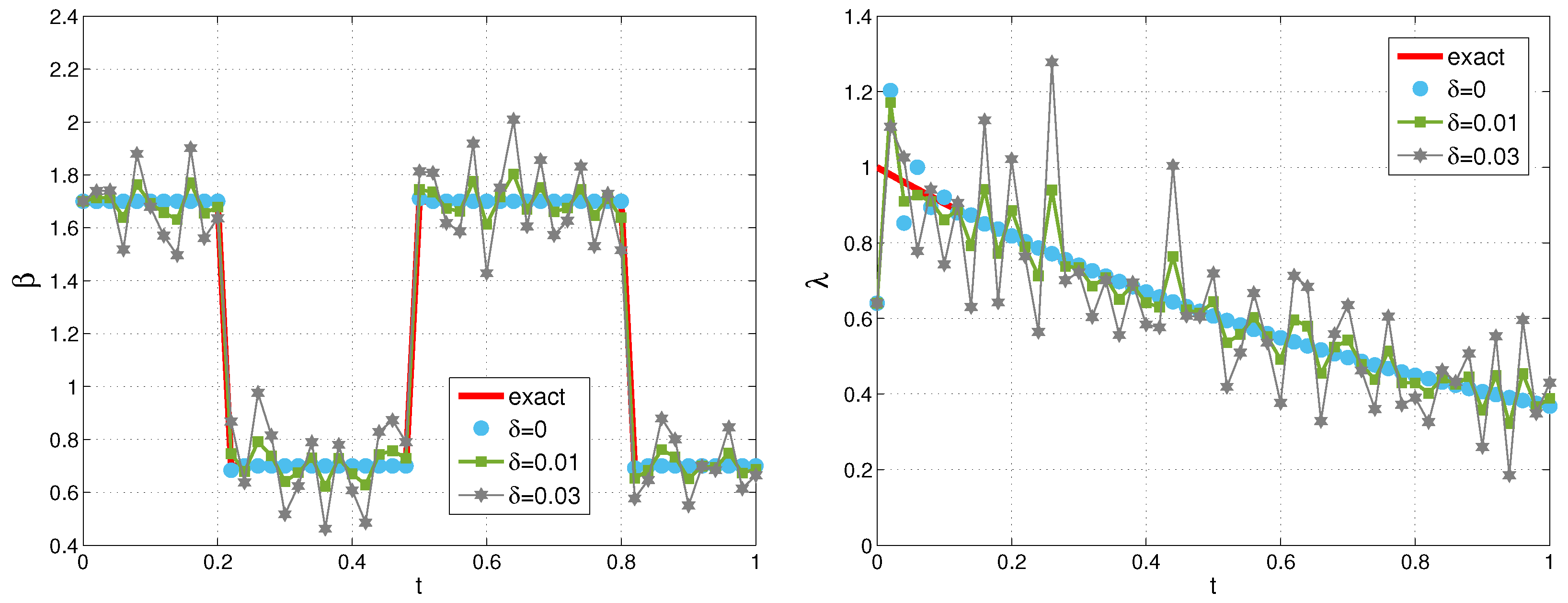
Results for different noise levels with $\alpha =0.5$, $x_1=0$, $x_2^{*}=0.5$, and  $I=N=50$ are depicted in Figure 1. As before, the approximate results for $\beta$ obtained by the present method are close to those reported in [35]. Moreover, the numerically recovered profiles of $\beta$ and $\lambda$ are in good agreement with the exact ones.

Further, we set (as in Example 3 of [36])

$$\beta \left(t\right)=\left\{\begin{array}{cc}1+\alpha ,\hfill & {\displaystyle 1<t\le \frac{1}{5},}\hfill \\ \alpha ,\hfill & {\displaystyle \frac{1}{5}<t<\frac{1}{2},}\hfill \\ 1+\alpha ,\hfill & {\displaystyle \frac{1}{2}\le t\le 45,}\hfill \\ \alpha ,\hfill & {\displaystyle \frac{4}{5}\le t\le 1.}\hfill \end{array}\right.$$

(26)

The function $r\left(t\right)$ is chosen, as before, in agreement with the given $\beta$ and the exact solution.

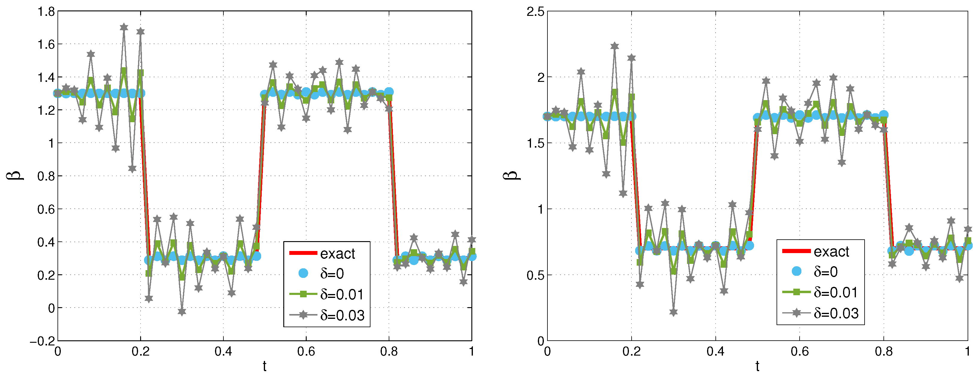
Computational results for $\alpha =0.3$, $\alpha =0.7$, $x_2^{*}=0.5$, and different noise levels are shown in Figure 2. Although, based on the consistency between the reconstructed and the exact profiles, the error appears slightly larger than that observed in [36], where only the Robin coefficient is identified, the numerical solution remains in very good agreement with the exact one. This behavior is expected, since our approach simultaneously reconstructs the two functions $\beta$ and $\lambda$, which generally leads to increased sensitivity of the solution.

Example 3 (Nonlinear problem, test 1). 

The test problem is Equations (1)–(3) with $k\left(u\right)=0.5u$. We consider the same solution u, coefficient b, and functions β and λ as in Example 2. The initial condition, Dirichlet boundary condition, and the functions $r\left(t\right)$ and $f(x,t)$ are chosen consistently with these data.

Computational results for $\alpha =0.5$, $x_2^{*}=0.5$, $I=200$, $N=100$, and different levels of noise are presented in

Table 3. Errors for different noise levels, $\alpha =0.5$; Example 3.

${\mathit{\delta }}_{\mathit{\phi }}$	0.0005	0.005	0.01	0.03	0.01	0.03	0.05	0.08
${\mathit{\delta }}_{\mathit{\psi }}$	0.0005	0.005	0.01	0.02	0.03	0.05	0.03	0.05
$\epsilon \left(\beta \right)$	0.0019	0.0145	0.0289	0.0758	0.0621	0.1153	0.1236	0.1999
${\epsilon }_r\left(\beta \right)$	7.5234 $\times {10}^{-4}$	0.0058	0.0116	0.0304	0.0248	0.0461	0.0495	0.0800
$\epsilon \left(\lambda \right)$	0.0211	0.0339	0.0559	0.1044	0.1544	0.2543	0.1543	0.2545
${\epsilon }_r\left(\lambda \right)$	0.0315	0.0506	0.0834	0.1558	0.2304	0.3796	0.2303	0.3799
$\mathcal{E}\left(u\right)$	9.6073 $\times {10}^{-4}$	0.0096	0.0192	0.0564	0.0573	0.0956	0.0941	0.1505
${\mathcal{E}}_r\left(u\right)$	3.9324 $\times {10}^{-4}$	0.0039	0.0079	0.0231	0.0234	0.0391	0.0385	0.0616
$m_a$	3.000	3.000	3.000	3.310	3.150	3.560	3.580	3.780

. The average number of iterations $m_a$ is also reported. We observe that the functions $\beta$ and $\lambda$ are recovered with sufficiently good accuracy within a small number of iterations, so that the solution u to attains optimal precision. Moreover, the number of iterations remains almost unchanged for different values of $\delta$, indicating that the method is stable with respect to noise.

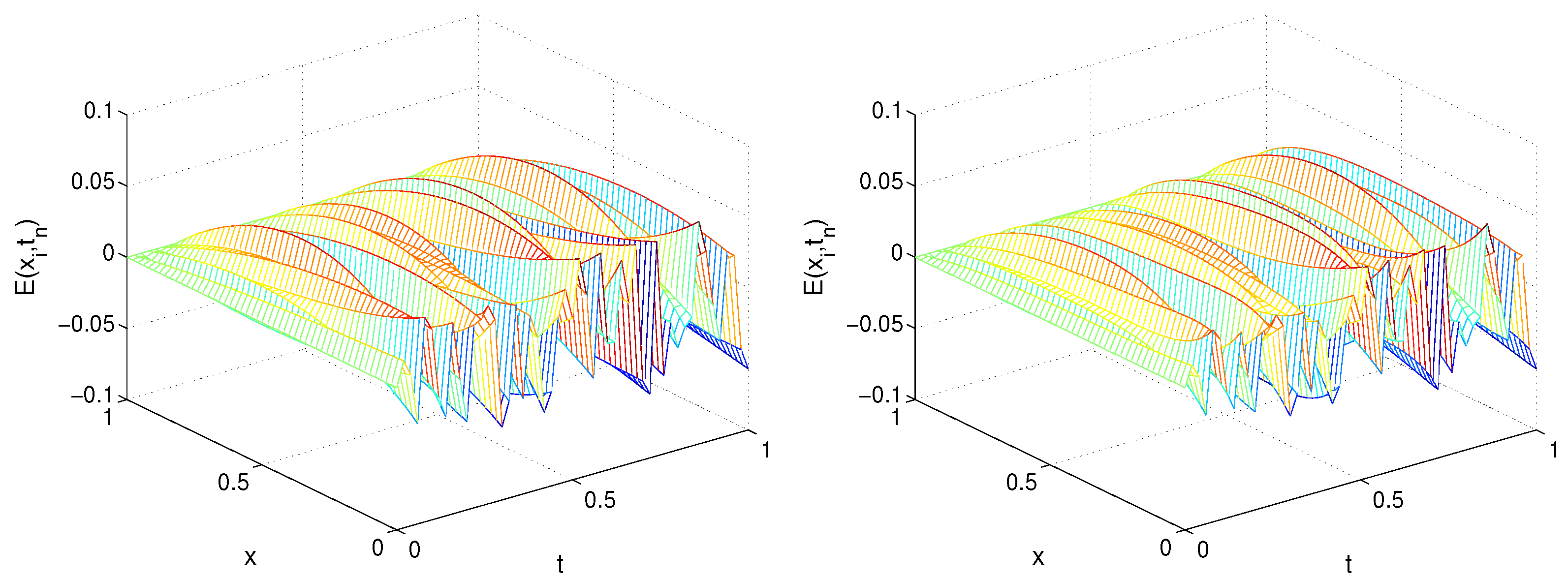
Now, we consider the function $\beta$, defined by Equation (26). In Figure 3 and Figure 4, we plot the recovered Robin coefficient $\beta$ and the right-hand side $\lambda$ for perturbed data, $I=N=50$, $x_2^{*}=0.5$, and $\alpha =0.3$ and $\alpha =0.7$. The average number of iterations corresponding to the simulations shown in Figure 3 and Figure 4 increases slightly as the noise level increases, ranging between $2.14$ and $3.54$. The reconstructed functions closely follow the shape of the exact ones. In Figure 5, we illustrate the error of the numerical solution for $\delta =0.3$. We observe that the solution u is less sensitive to the fractional order compared to the reconstructed functions $\beta$ and $\lambda$. The largest errors occur at the internal point and near the Robin boundary. The locally increased error near the interior measurement point can be attributed to the direct propagation of measurement noise through the reconstruction of Equation (13) and subsequent solution decomposition Equation (9), which is typical for inverse problems relying on local (pointwise) measurements.

Example 4 (Nonlinear problem, test 2). 

The test problem is Equations (1)–(3) with $k\left(u\right)=u^3$. Let $b=1$, $\beta \left(t\right)=2t^2+3t+2$, $\lambda \left(t\right)={\left[E_{\alpha }(-t^{\alpha })\right]}^4$, ${\displaystyle u(x,t)=E_{\alpha }(-t^{\alpha })cos\frac{\pi x}{2}}$, where $E_{\alpha }$ denotes the Mittag-Leffler function, and ${\displaystyle f\left(x\right)=\frac{{\pi }^2}{4}{cos}^2\frac{\pi x}{2}\left(1-4sin\frac{\pi x}{2}\right)sin\frac{\pi x}{2}}$. The input data $f(x,t)$, $r\left(t\right)$, $g\left(t\right)$, and $u_0\left(t\right)$ are chosen consistently with the exact solution and the functions $\beta \left(t\right)$ and $\lambda \left(t\right)$.

In

Table 4. Errors for different noise levels, $\alpha =0.5$; Example 4.

${\mathit{\delta }}_{\mathit{\phi }}$	0.0005	0.005	0.01	0.03	0.01	0.03	0.05	0.08
${\mathit{\delta }}_{\mathit{\psi }}$	0.0005	0.005	0.01	0.02	0.03	0.05	0.03	0.05
$\epsilon \left(\beta \right)$	0.0049	0.0135	0.0257	0.0716	0.0396	0.0876	0.1183	0.1910
${\epsilon }_r\left(\beta \right)$	6.9636 $\times {10}^{-4}$	0.0019	0.0037	0.0102	0.0057	0.0125	0.0169	0.0273
$\epsilon \left(\lambda \right)$	0.0243	0.0263	0.0348	0.0591	0.0874	0.1439	0.0864	0.1432
${\epsilon }_r\left(\lambda \right)$	0.0972	0.1052	0.1392	0.2364	0.3496	0.5756	0.3456	0.5728
$\mathcal{E}\left(u\right)$	0.0078	0.0075	0.0113	0.0260	0.0355	0.0593	0.0864	0.0641
${\mathcal{E}}_r\left(u\right)$	0.0078	0.0075	0.0113	0.0260	0.0355	0.0593	0.0864	0.0641
$m_a$	3.000	3.090	3.260	3.700	3.650	3.940	3.880	4.050

, we present the errors of the identified functions $\beta$ and $\lambda$ as well as of the solution u, together with the average number of iterations, computed for $x_2^{*}=0.5$, $\alpha =0.5$, $I=200$, $N=100$. As in Example 3, we observe that the convergence is attained within a small number of iterations, and that the method is stable with respect to noise, since the number of iterations does not increase significantly as $\delta$ increases.

Now, we consider the following Robin boundary coefficient profile:

$$\beta \left(t\right)=\left\{\begin{array}{cc}t,\hfill & {\displaystyle 0\le t\le \frac{1}{2},}\hfill \\ 1-t,\hfill & {\displaystyle \frac{1}{2}<t\le 1}\hfill \end{array}\right.$$

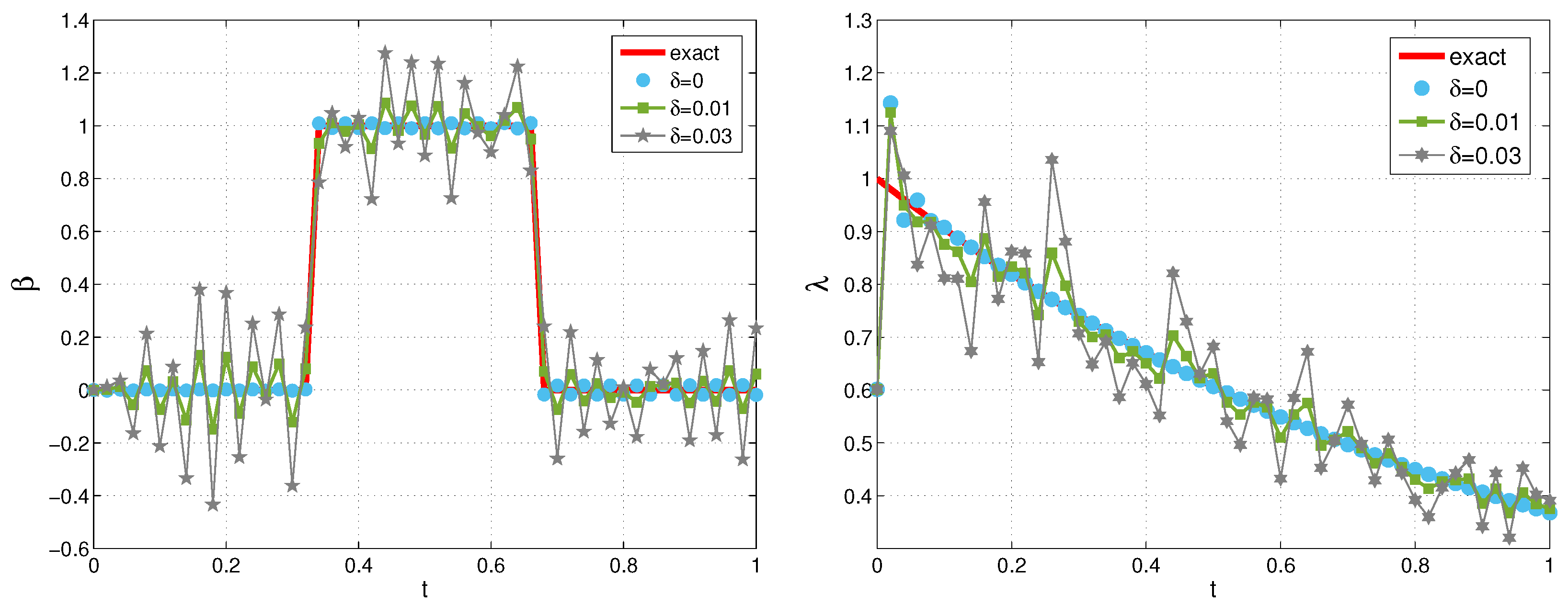
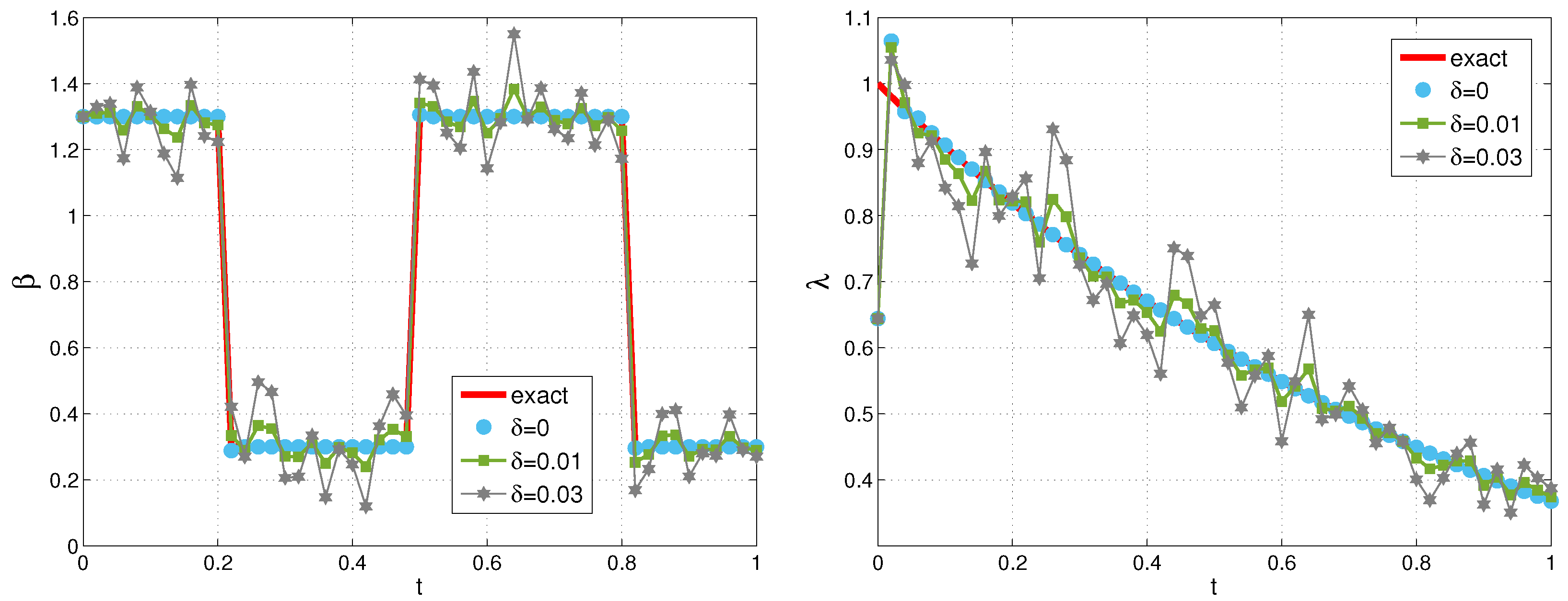
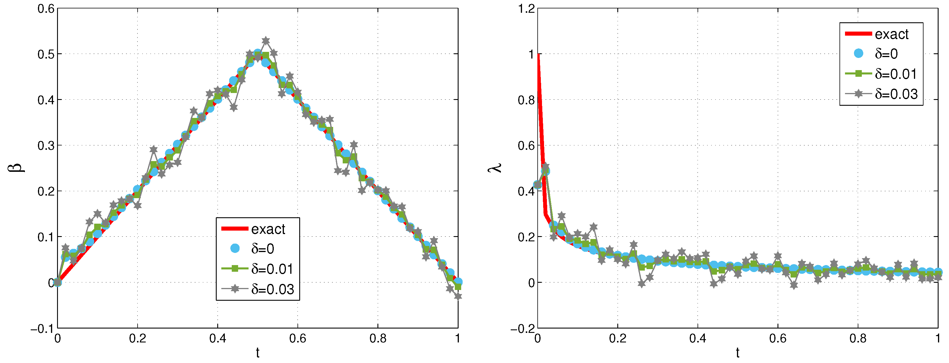
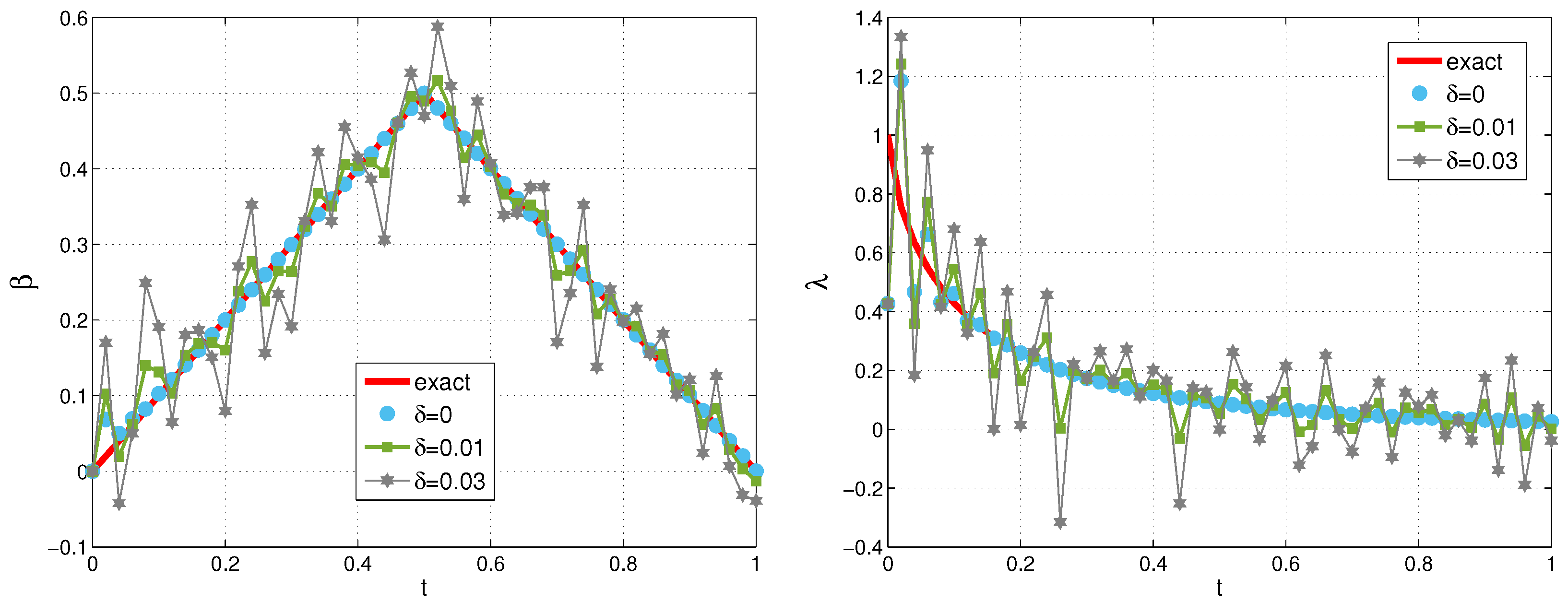
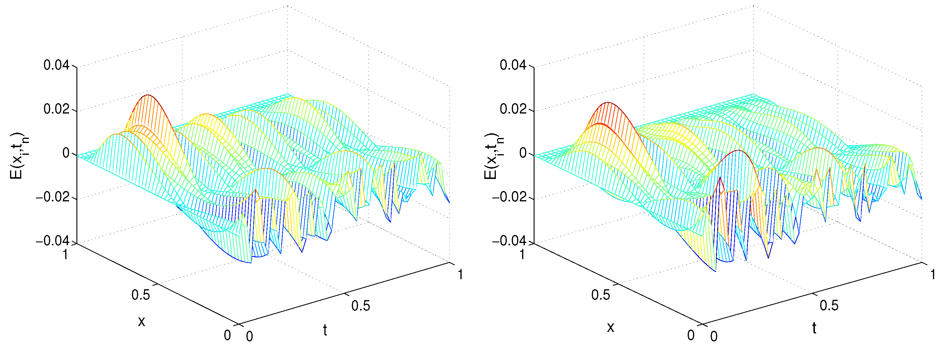
The function $r\left(t\right)$ is chosen according to $\beta \left(t\right)$ and the exact solution. On Figure 6 and Figure 7, we present the exact functions $\beta \left(t\right)$ and $\lambda \left(t\right)$, together with their approximations for different noise levels, $\alpha =0.3$, $\alpha =0.7$, and $I=N=50$, $x_2^{*}=0.5$. For each run, the computational process attains the desired accuracy within a small number of iterations, ranging between $3.12$ and $4.7$, depending on $\alpha$ and $\delta$. Figure 8 illustrates the error $E(x_i,t_n)$, $i=0,1,\dots ,I$, $n=0,1,\dots ,N$ of the numerical solution $u_i^n$ for $\alpha =0.3$, $\alpha =0.7$ and $\delta =0.3$. We observe that the error profiles are very similar for both values of $\alpha$ and are therefore not strongly sensitive to the fractional order. Moreover, the results indicate that the functions $\beta$ and $\lambda$ are identified with sufficiently good accuracy even in the presence of noisy data, leading to acceptable accuracy of the numerical solution u.

6. Conclusions

In this paper, we have presented numerical approaches for the simultaneous identification of a time-dependent right-hand side and a Robin boundary coefficient in linear and quasilinear time-fractional reaction–diffusion problems. The correctness of the proposed method is shown in the sense that the existence and uniqueness of the reconstructed functions at the semi-discrete level are established, and robustness with respect to data perturbations is investigated numerically through noise-contaminated experiments.

The numerical results demonstrate that, even in the presence of noisy data, the unknown functions are reconstructed with sufficiently good accuracy so that the numerical solution is computed with satisfactory precision. For the nonlinear problem, an iterative scheme based on quasilinearization is developed. It is shown that convergence is achieved within a small number of iterations and that the method is stable with respect to noise, since the number of iterations does not increase significantly as the noise level increases.

Future work will address inverse problems for more general fractional models, in particular space–time fractional diffusion and the recovery of the fractional order from measurement data.

References

1. Alifanov, O.M.; Artioukhine, E.A.; Rumyantsev, S.V. Extreme Methods for Solving Ill-Posed Problems with Applications to Inverse Heat Transfer Problems; Begell House: Danbury, CT, USA, 1995. [Google Scholar]
2. Hasanov, A.H.; Romanov, V.G. Introduction to Inverse Problems for Differential Equations; Springer: Cham, Switzerland, 2017. [Google Scholar]
3. Isakov, V. Inverse Problems for Partial Differential Equations, 3rd ed.; Springer: Cham, Switzerland, 2017; 406p. [Google Scholar]
4. Kabanikhin, S.I. Inverse and Ill-Posed Problems; DeGruyer: Berlin, Germany, 2011. [Google Scholar]
5. Lesnic, D. Inverse Problems with Applications in Science and Engineering, 1st ed.; Chapman and Hall/CRC: New York, NY, USA, 2021. [Google Scholar]
6. Samarskii, A.A.; Vabishchevich, P.N. Numerical Methods for Solving Inverse Problems in Mathematical Physics; de Gruyter: Berlin, Germany, 2007; 438p. [Google Scholar]
7. Colton, D.; Kress, R. Inverse Acoustic and Electromagnetic Scattering Theory, 3rd ed.; Springer: New York, NY, USA, 2013. [Google Scholar]
8. Orlande, H.R.B. Inverse Heat Transfer: Fundamentals and Applications, 2nd ed.; CRC Press: Boca Raton, FL, USA, 2021; 297p. [Google Scholar]
9. Metzler, R.; Klafter, J. The random walk’s guide to anomalous diffusion: A fractional dynamics approach. Phys. Rep. 2000, 339, 1–77. [Google Scholar] [CrossRef]
10. Podlubny, I. Fractional Differential Equations, Mathematics in Science and Engineering; Academic Press: San Diego, CA, USA, 1999; Volume 198. [Google Scholar]
11. Luchko, Y. Some uniqueness and existence results for the initial-boundary value problems for the generalized time-fractional diffusion equation. Comput. Math. Appl. 2010, 59, 1766–1772. [Google Scholar] [CrossRef]
12. Luchko, Y. Comparison principles for the time-fractional diffusion equations with Neumann and Robin boundary conditions. Fract. Calc. Appl. Anal. 2023, 26, 1504–1544. [Google Scholar] [CrossRef]
13. Kubica, A.; Yamamoto, M. Initial-boundary value problems for fractional diffusion equations with time-dependent coefficients. Fract. Calc. Appl. Anal. 2018, 21, 276–311. [Google Scholar] [CrossRef]
14. Wang, H.; Yang, D. Well-posedness of variable-coefficient conservative fractional diffusion equations. SIAM J. Numer. Anal. 2013, 51, 1088–1107. [Google Scholar] [CrossRef]
15. Kemppainen, J. Existence and uniqueness of the solution for a time-fractional diffusion equation with Robin boundary condition. In Abstract and Applied Analysis; Hindawi Publishing Corporation: New York, NY, USA, 2011; Volume 2011, pp. 1–11. [Google Scholar]
16. Zacher, R. Global strong solvability of a quasilinear subdiffusion problem. J. Evol. Equ. 2012, 12, 813–831. [Google Scholar] [CrossRef]
17. Krasnoshchok, M. Classical solutions of time-fractional quasilinear reaction-diffusion systems. Ukr. Math. J. 2025, 77, 212–230. [Google Scholar] [CrossRef]
18. Gal, C.G.; Warma, M. Fractional-in-Time Semilinear Parabolic Equations and Applications, 1st ed.; Springer: Cham, Switzerland, 2020; 184p. [Google Scholar]
19. Hazanee, A.; Lesnic, D.; Ismailov, M.I.; Kerimovc, N.B. An inverse time-dependent source problem for the heat equation with a non-classical boundary condition. Appl. Math. Model. 2015, 39, 6258–6272. [Google Scholar] [CrossRef]
20. Ismailov, M.I.; Kanca, F.; Lesnic, D. Determination of a time-dependent heat source under nonlocal boundary and integral overdetermination conditions. Appl. Math. Comput. 2011, 218, 4138–4146. [Google Scholar] [CrossRef]
21. Woodbury, K.A.; Najafi, H.; de Monte, F.; Beck, J.V. Inverse Heat Conduction: Ill-Posed Problems; John Wiley & Sons, Inc.: New York, NY, USA, 2023; 324p. [Google Scholar]
22. Huntul, M.J. Identification of the unknown heat source terms in a 2D parabolic equation. J. King Saud Univ. Sci. 2021, 67, 3681–3699. [Google Scholar] [CrossRef]
23. Shivanian, E.; Jafarabadi, A.; Chegini, T.G.; Dinmohammadi, A. Analysis of a time-dependent source function for the heat equation with nonlocal boundary conditions through a local meshless procedure. Comp. Appl. Math. 2025, 44, 282. [Google Scholar] [CrossRef]
24. Shivanian, E.; Jafarabadi, A.; Fairooz, M.Z.; Dinmohammadi, A. Solving the inverse problem of time-dependent heat source identification with non-classical boundary conditions. J. Comput. Appl. Math. 2026, 476, 17074. [Google Scholar] [CrossRef]
25. Koleva, M.N.; Vulkov, L.G. Source identification for a two-dimensional parabolic equation with an integral constraint. Mathematics 2025, 13, 1876. [Google Scholar] [CrossRef]
26. Asl, N.A.; Rostamy, D. Identifying an unknown time-dependent boundary source in time-fractional diffusion equation with a non-local boundary condition. J. Comput. Appl. Math. 2019, 355, 36–50. [Google Scholar] [CrossRef]
27. Lyu, K.; Cheng, H. Inverse source problem for the time-space fractional diffusion equation involving the fractional Sturm-Liouville operator. Commun. Nonlinear Sci. Numer. Simul. 2025, 146, 108772. [Google Scholar] [CrossRef]
28. Durdiev, D.K.; Sultanov, M.A.; Rahmonov, A.A.; Nurlanuly, Y. Inverse problems for a time-fractional diffusion equation with unknown right-hand side. Progr. Fract. Differ. Appl. 2023, 9, 639–653. [Google Scholar]
29. Derbissaly, B.; Kirane, M.; Sadybekov, M. Inverse source problem for two-term time-fractional diffusion equation with nonlocal boundary conditions. Chaos Solitons Fractals 2024, 183, 14897. [Google Scholar] [CrossRef]
30. Jin, B.; Rundell, W. A tutorial on inverse problems for anomalous diffusion processes. Inverse Probl. 2015, 31, 035003. [Google Scholar] [CrossRef]
31. Jin, B.; Lu, X. Numerical identification of a Robin coefficient in parabolic problems. Math. Comput. 2012, 81, 1369–1398. [Google Scholar] [CrossRef]
32. Ma, Y.-J. Reconstruction of a Robin coefficient by a predictor-corrector method. Math. Probl. Eng. 2015, 2015, 496587. [Google Scholar] [CrossRef]
33. Slodička, M.; Keer, R.V. Determination of a Robin coefficient in semilinear parabolic problems by means of boundary measurements. Inverse Probl. 2002, 18, 139. [Google Scholar] [CrossRef]
34. Rashedia, K.; Baharifardb, F. A meshfree regularization method for recovering a time-dependent Robin coefficient in one-dimensional transient heat conduction. Int. J. Nonlinear Anal. Appl. 2024, 15, 11–22. [Google Scholar]
35. Wang, J.-G.; Ran, Y.-H.; Yuan, Z.-B. Uniqueness and numerical scheme for the Robin coefficient identification of the time-fractional diffusion equation. Comput. Math. Appl. 2018, 75, 4107–4114. [Google Scholar] [CrossRef]
36. Wei, T.; Wang, J.-G. Determination of Robin coefficient in a fractional diffusion problem. Appl. Math. Model. 2016, 40, 7948–7961. [Google Scholar] [CrossRef]
37. Shi, C.; Cheng, H. Identify the Robin coefficient in an inhomogeneous time-fractional diffusion-wave equation. J. Comput. Appl. Math. 2023, 434, 115337. [Google Scholar] [CrossRef]
38. Mondal, S. Convergence rates for identification of Robin coefficient from terminal observations. arXiv 2024, arXiv:2304.00726. [Google Scholar] [CrossRef]
39. Cao, X.; Lesnic, D. Simultaneous identification and reconstruction of the space-dependent reaction coefficient and source term. J. Inverse Ill-Posed Probl. 2021, 29, 867–894. [Google Scholar] [CrossRef]
40. Qiao, H.; Li, X.; Liu, J. Simultaneous identification of the unknown source term and initial value for the time fractional diffusion equation with local and nonlocal operators. Chaos Solitons Fractals 2024, 189, 115601. [Google Scholar] [CrossRef]
41. Kamynin, V.L. The inverse problem of the simultaneous determination of the right-hand side and the lowest coefficient in parabolic equations with many space variables. Math. Notes 2015, 97, 349–361. [Google Scholar] [CrossRef]
42. Mehraliyev, F.; Huntul, M.J.; Azizbayov, E.I. Simultaneous identification of the right-hand side and time-dependent coefficients in a two-dimensional parabolic equation. Math. Model. Anal. 2024, 29, 90–108. [Google Scholar] [CrossRef]
43. Abdelhamid, T.; Deng, X.; Chen, R. A new method for simultaneously reconstructing the space-time dependent Robin coefficient and heat flux in a parabolic system. Int. J. Numer. Anal. Model. 2017, 14, 893–915. [Google Scholar]
44. Jiang, D.; Li, Z. Hopf’s lemma and uniqueness of simultaneously determining source profile and Robin coefficient in a fractional diffusion equation by interior data. Inverse Probl. Imaging 2024, 18, 1121–1141. [Google Scholar] [CrossRef]
45. Cannon, J.R. The One-Dimensional Heat Equation; Cambridge University Press: Cambridge, UK, 1984. [Google Scholar]
46. Cahill, D.G.; Braun, P.V.; Chen, G.; Clarke, D.R.; Fan, S.; Goodson, K.E.; Keblinski, P.; King, W.P.; Mahan, G.D.; Majumdar, A.; et al. Nanoscale thermal transport. Appl. Phys. Rev. 2014, 1, 011305. [Google Scholar] [CrossRef]
47. Slodička, M.; Lesnic, D.; Onyango, T.T.M. Determination of a time-dependent heat transfer coefficient in a nonlinear inverse heat conduction problem. Inverse Probl. Sci. Eng. 2009, 18, 65–81. [Google Scholar] [CrossRef]
48. Marusić-Paloka, E.; Pažanin, I. The Robin boundary condition for modelling heat transfer. Proc. R. Soc. A 2024, 480, 20230850. [Google Scholar] [CrossRef]
49. Chmielowska, A.; Brociek, R.; Slota, D. Reconstructing the Heat Transfer Coefficient in the Inverse Fractional Stefan Problem. Fractal Fract. 2025, 9, 43. [Google Scholar] [CrossRef]
50. Pyatkov, S.G. Identification of the heat transfer coefficient using an inverse heat conduction model. arXiv 2024, arXiv:2401.01551. [Google Scholar] [CrossRef]
51. Alikhanov, A.A. A new difference scheme for the time fractional diffusion equation. J. Comput. Phys. 2015, 280, 424–438. [Google Scholar] [CrossRef]
52. Tatar, S.; Ulusoy, S. An inverse problem for a nonlinear diffusion equation with time-fractional derivative. J. Inverse Ill-Posed Probl. 2017, 25, 185–193. [Google Scholar] [CrossRef]
53. Bellman, R.; Kalaba, R. Quasilinearization and Nonlinear Boundary-Value Problems; Elsevier Publishing Company: New York, NY, USA, 1965. [Google Scholar]
54. Koleva, M.N.; Vulkov, L.G. Fitted finite volume method for unsaturated flow parabolic problems with space degeneration. In Large-Scale Scientific Computing; Lirkov, I., Margenov, S., Eds.; Lecture Notes in Computer Science; Springer International Publishing: Cham, Switzerland, 2022; Volume 13127. [Google Scholar]
Figure 1. Exact  β ( t )  and its approximations (left), exact  λ ( t )  and its approximations (right) for different levels of noise,  α = 0.5 ; Example 2.
Mathematics 14 00324 g001
Figure 2. Exact  β ( t )  and its approximations for  α = 0.3  (left) and  α = 0.7  (right) for different levels of noise; Example 2.
Mathematics 14 00324 g002
Figure 3. Exact  β ( t )  and its approximations (left) and exact  λ ( t )  and its approximations (right) for different levels of noise,  α = 0.3 ; Example 3.
Mathematics 14 00324 g003
Figure 4. Exact  β ( t )  and its approximations (left) and exact  λ ( t )  and its approximations (right) for different levels of noise,  α = 0.7 ; Example 3.
Mathematics 14 00324 g004
Figure 5. Error  E ( x i , t n ) i = 0 , 1 , , I n = 0 , 1 , , I  of the numerical solution  u i n  for  δ = 0.3 α = 0.3  (left) and  α = 0.7  (right); Example 3.
Mathematics 14 00324 g005
Figure 6. Exact  β ( t )  and its approximations (left) and exact  λ ( t )  and its approximations (right) for different levels of noise,  α = 0.3 ; Example 4.
Mathematics 14 00324 g006
Figure 7. Exact  β ( t )  and its approximations (left) and exact  λ ( t )  and its approximations (right) for different levels of noise,  α = 0.7 ; Example 4.
Mathematics 14 00324 g007
Figure 8. Error  E ( x i , t n ) i = 0 , 1 , , I n = 0 , 1 , , I  of the numerical solution  u i n  for  δ = 0.3 α = 0.3  (left) and  α = 0.7  (right); Example 4.
Mathematics 14 00324 g008