Article

Robust Integral Optimal Sliding Mode Control Design for Electromagnetic Levitation System with Matched Uncertainties

1
Department of Electrical & Electronic Engineering Technology, University of Johannesburg, Johannesburg 2094, South Africa
2
Department of Human Anatomy and Physiology, Faculty of Health Sciences, University of Johannesburg, Johannesburg 2094, South Africa
3
Department of Electrical Engineering, Malaviya National Institute of Technology, Jaipur 302017, India
*
Author to whom correspondence should be addressed.
Mathematics 2026, 14(2), 229; https://doi.org/10.3390/math14020229
Submission received: 10 September 2025 / Revised: 19 October 2025 / Accepted: 22 October 2025 / Published: 8 January 2026
(This article belongs to the Special Issue Advances in Control Systems and Automatic Control, 2nd Edition)

Abstract

Recently, there has been a rapid increase in the demand for magnetic levitation systems. Since they are utilized in many levitation-based systems, one such application is in magnetic levitated (Maglev) trains. Moreover, these systems are complicated to control due to their nonlinear characteristics, susceptibility to external disturbances, and model uncertainties. This article proposes an enhanced integral sliding mode control (ISMC) strategy with a robust optimal framework designed for electromagnetic levitation systems (EMLSs). Traditional sliding mode control (SMC) often suffers from a high-frequency phenomenon in the input, thereby necessitating the development of a more robust controller. This requirement is addressed through the implementation of a comprehensive integral robust optimal sliding mode control strategy. The proposed controller effectively mitigates the chattering phenomenon while simultaneously enhancing the system’s robustness against uncertainties. The robust optimal approach is specifically designed to handle the matched uncertainties inherent in the system dynamics, thereby facilitating an appropriate feedback control mechanism. The Hamilton–Jacobi–Bellman (HJB) equation is used to achieve the robust control design. This feedback control is integrated with the ISMC to execute the desired control action effectively. The simulation results highlight the effectiveness of the proposed control scheme, presenting a comparative analysis of performance indices, including integral time absolute error (ITAE), integral absolute error (IAE), integral squared error (ISE), and integral time squared error (ITSE). These indices collectively underscore the robustness of the control design.

1. Introduction

It is a fact that all physical systems are inherently nonlinear. This has become one of the primary reasons for research over the past several decades. Rotary inverted pendulums, ball and beam systems, electromagnetic levitation systems, and many more are benchmark problems that strongly exhibit the property of nonlinearity. As the EMLS has numerous applications in different areas, such as magnetic bearings, robots, spacecraft, and magnetic levitation (Maglev) trains, the control law designed to tackle the system’s nonlinear behavior must be stable and robust. Magnetic levitation uses the property of magnetic attraction or repulsion to keep an object suspended in the air. Recently, many controllers have been developed to handle the nonlinear characteristics of the system; however, the need now is to develop more techniques beyond existing ones to provide better stability and robustness to the system.
The latest findings have shown that various linear and nonlinear controllers have been developed to address the challenges of stability and robustness in the EMLS in the presence of uncertainties. Moreover, linear controllers utilize the linearized model of the system, which cannot provide the robustness required to compensate for the nonlinearities present in the actual system model. One of the nonlinear controllers that offer excellent tracking against uncertainties is the sliding mode controller (SMC). The sliding mode controller has a wider range of applications, such as in mechanical systems [1], chemical processes [2], electrical systems [3], robotics [4], automobiles [5], and aeronautics [6]. A sliding mode control and proportional–integral (PI) plus lead compensator are designed in [7], and the SMC performs better than the classical PI controller. Moreover, the current dynamics are neglected, and the desired ball position is restricted to 1 mm. A dual-axis Maglev positioning system represents an advanced magnetic levitation technology that has been designed employing an adaptive sliding mode controller, as referenced in [8]. A sliding mode control strategy, which utilizes a proportional–integral switching surface, is proposed in [9], in which a comparative analysis of the performance of the designed controller against that of a feedback linearized controller is discussed. Furthermore, in [10], a methodology for determining uncertainty boundaries through the application of artificial neural networks, which is integrated into the sliding mode control of the Maglev system is introduced.
The SMC equivalence approach was integrated with the reaching law method in [11] to propose a variable structure controller (VSC) for the Maglev system. In a separate study, developed in [12], a static SMC is proposed for the electromagnetic levitation system. Furthermore, in [13], a second-order sliding mode control strategy for an EMLS is proposed, employing the super-twisting algorithm. In [14], SMC is specifically designed for a second-order electromagnetic levitation system, and the performance outcomes are compared with those of a conventional PID controller. The findings indicate that the SMC outperforms the traditional control approach. Additionally, in [15], a PID-based Q-learning method designed to enhance the stability of the magnetic levitation system. Moreover, a non-singular terminal sliding mode control with finite-time convergence is developed for high-speed maglev trains, with disturbance estimation accomplished via a nonlinear observer as described in [16].
Cascade control is developed for the Maglev system to control the levitation. The proposed method employs the SMC and fuzzy PID controller to provide the necessary control action [17]. A genetic algorithm-based ST-SMC is designed for the Maglev system. The proposed technique also incorporates the genetic algorithm-based sliding mode control. Since SMC suffers from the problem of high-frequency oscillations, the super-twisting sliding mode control is designed to handle the unwanted chattering issue [18]. In [19], an extended state observer (ESO) and an ISMC are used to develop the proposed control technique. The designed approach eliminates all uncertainties without employing upper-bound uncertainty knowledge. A dynamic Petri fuzzy neural network system-based intelligent controller is designed for the Maglev system [20]. The ISMC improves the system convergence rate and ensures robustness. A radial basis neural network SMC is designed in [21] for the EMLS. The neural network needs the Jacobian model; however, this need is eliminated by using the SMC.
Another control technique, model predictive control, has been extensively studied for the electromagnetic levitation system. Zhang et al. [22] proposed the integration of nonlinear and linear model predictive control for state feedback and constraint handling. Nonlinear model predictive control for the EMLS with Lyapunov stability has been studied [23,24]. A linear model predictive control with a neural network is designed to handle the uncertainties in the electromagnetic levitation system [25]. A reinforcement learning-based model predictive control is designed to control the electromagnetic levitation system. The control scheme basically adapts the control policy in a real-time scenario. An adaptive linear disturbance rejection-based sliding mode control technique is discussed [26]. This technique combines particle swarm optimization and adaptive disturbance rejection with sliding mode control for optimal parameter selection in the EMLS. The adaptive fast terminal and non-singular terminal-based sliding mode control is proposed for a nonlinear and uncertain maglev system [27,28,29]. The proposed techniques offer better disturbance rejection, improved dynamic performance, faster convergence, and enhanced tracking. However, these techniques come with computational burden, precise modeling, difficulty in online optimization, and high switching efforts.
Some researchers have investigated the optimal sliding mode control technique, which combines a sliding mode control method and an optimal control idea. The design of optimal sliding mode control incorporates two primary concepts: the optimization of disturbance attenuation [30] and the enhancement of tracking performance for reference signals [31,32]. Given that sliding mode control is significantly challenged by the issue of high-frequency oscillations, which can lead to system instability, it is essential to develop a more robust controller for the EMLS. The ISMC eliminates the problem of the reaching phase and the chattering effect. The purpose of introducing robust optimal control in the nominal control action is to achieve the desired position of the ball with negligible steady-state error. Since traditional optimal controllers are sensitive to model mismatch, they cannot perform optimally. Therefore, the robust optimal control technique is introduced to enhance the nominal control of the electromagnetic levitation system. This approach computes the optimal gain by addressing potential matched uncertainties. Consequently, IOSMC will enhance robustness and tracking capabilities for the EMLS in the presence of external disturbances and variations in system parameters.

2. Contribution and Manuscript Framework

  • This article presents a robust integral optimal sliding mode control strategy developed for an electromagnetic levitation system. The conventional sliding mode control methodology encounters challenges such as high-frequency chattering and exhibits limited robustness towards uncertainties and parameter variations.
  • To address these issues, an integral sliding mode is introduced, in which robust optimal control gains is integrated within the reaching phase. This integration not only reduces the chattering effects by smoothing the switching control action but also improves disturbance rejection and robustness towards uncertainties.
  • In the proposed approach, the control input comprises nominal control and discontinuous control. The nominal control action is formulated using a robust optimal design based on the Hamilton–Jacobi–Bellman (HJB) formulation, which evidently integrates uncertainty bounds and system parameter perturbations into the performance function. The discontinuous component ensures invariance of the sliding manifold in the presence of external disturbances.
  • The controller gain is calculated for matched uncertainties, ensuring the global asymptotic stability and finite-time convergence of the system states, thereby improving tracking of desired positions and eliminating steady-state errors. Therefore, the integration of integral sliding mode control with a robust optimal technique provides enhanced robustness, stability, and reduced control effort requirements compared to sliding mode control.
The subsequent sections of this article are organized as follows:
  • Section 3 presents the development of the nonlinear state equation of the EMLS.
  • Section 4 focuses on controller design and is further divided into three subsections: Section 4.1 addresses the design of sliding mode control, Section 4.2 elaborates on integral sliding mode control, and Section 4.3 discusses the optimal control design.
  • Section 5 highlights the simulation results and discussion on the performance of the EMLS.
  • Finally, Section 6 provides a conclusion that summarizes the proposed work and its findings.

3. Model of EMLS

The discussion in this part examines the complex mathematical modeling associated with a voltage-controlled electromagnetic levitation system. This system utilizes a state-space model, which offers a robust and flexible framework for investigation, modeling, and control of the dynamics inherent to the levitation mechanism. Figure 1 highlights the EMLS model; the fundamental aim of the system is to keep the position of the ball at the desired value. The state x a refers to the position of the ball. The desired position of the ball can be obtained by changing the control effort, which is the coil voltage v c .
When the voltage v c is applied, the current in the coil starts to flow, called i c , in the system. This coil current produces the attractive magnetizing force that is capable of lifting the steel ball upward. The working principle of the EMLS is based on the electrical and mechanical phenomena, which employ two important laws: Newton’s law of motion and Kirchhoff’s voltage law. Both laws work together to enable better control of the electromagnetic levitation system [33].
According to Newton’s law of motion, the equation for the motion of the steel ball is given by Equation (1).
d 2 x a d t 2 = g e G e i c 2 2 m b x a 2
where m b is the weight of the ball, g e is the acceleration due to gravity acting on the ball, and G e is the electromagnetic constant.
To obtain the equation of the voltage applied to the circuit, Kirchhoff’s voltage law (KVL) is applied to the system. The equation of the coil voltage is shown in Equation (2).
v c ( t ) = ( r c + r s ) i c ( t ) + l c d i c ( t ) d t
where r c is the resistance of the coil, in Ohms, r s is the sensing resistance, in Ohms, and l c is the inductance of the coil, in Henrys. The state-space model of the EMLS is obtained by rearranging Equations (1) and (2), which is shown in Equation (3).
x a ˙ x b ˙ x c ˙ = x b g e G e 2 m b x c x a 2 r c + r s l c x c + 0 0 1 l c u
y = x a 0 0
where x a is the position of the steel ball, x b is the velocity of the steel ball, and x c is the current in the coil. The linearized model of the EMLS is obtained at the equilibrium point x 0 , u 0 . Hence, the linearized model is shown below:
A = 0 1 0 G e m b x c 0 2 x a 0 3 0 G e m b x c 0 x a 0 2 0 0 r c + r s l c B = 0 0 1 l c
In the voltage-controlled system, the nonlinearity arises from the state of the system, as highlighted in Equation (1). The one unstable open-loop pole lies on the right-hand side of the s-plane and is obtained while keeping the ball position at 9 mm and current at 1.28 A in the linearized model shown in Equation (4). This presents a challenge in maintaining stability and control in the levitation process.

4. Controller Design

The goal of this part is to develop different controllers to control the position of the steel ball of the EMLS, while ensuring the global stability and handling the parametric as well as the external disturbances to which the EMLS is subjected. In the subsequent part of this section, different controller designs are discussed in detail.

4.1. Sliding Mode Control

SMC is an effective method for dealing with sudden and significant changes that occur in the system. The SMC can be developed in two stages. The first stage is designing the switching state and the second stage is developing the control mechanism that will force the system trajectories to reach and slide on the switching surface. The reachability state is an important criterion in the SMC, which ensures the existence of the sliding mode. Robustness against the uncertainties is assured once the sliding is achieved and maintained. Consider the system shown in Equation (5)
x ˙ = A x + B u
where x R n × 1 is the state vector, A is the system matrix A R n × n , B is the input matrix B R n × m , and u represents the input vector u R m × 1 . The main objective lies in designing the switching surface for the SMC, for which it is assumed that the system matrix A and control matrix B are controllable and in standard form. Equation (6) represents the system in the normal form.
x ¯ ˙ = A a a A a b A b a A b b x ¯ + 0 B u u
where A a a R ( n m ) × ( n m ) , A a b R ( n m ) × m , A b a R n × ( n m ) , A b b R m × m , and B 2 R m × m . Equation (7) highlights the assumed switching surface S S u ,
S S u = N x ¯ = 0
where N = [ N 1 I ] and N 1 R m × ( n m ) . Hence, Equation (8) showcases the sliding phase
S u = N 1 I x 1 ¯ x 2 ¯ = 0
where x 1 ¯ R ( n m ) × 1 and x 2 ¯ R m × 1 .
Using Equation (8), x 2 ¯ = N 1 x 1 ¯ . Furthermore, utilising Equation (6) and the equation of x 2 ¯ , x 1 ¯ ˙ is given by Equation (9)
x 1 ¯ ˙ = A a a A b a N 1 x 1 ¯
The value of N 1 is so chosen such that x 1 ¯ ˙ is Hurwitz.
Assume that x 1 d , x 2 d , and x 3 d are the desired values of the steel ball position, velocity of the ball, and coil current. The equations of the errors in the terms of the desired values of the position of the ball, velocity of the ball, and coil current are given by Equations (10)–(12).
e p = x a x a d
e v = x b x b d
e c = x c x c d
where e p is the position error of the ball, e v is the velocity error of the ball, and e c is the error of the coil current. The control effort in the SMC has two different components: The first control effort component is called the continuous component, denoted as u c c , which is responsible for driving the motion of the system and subsequently improves its performance on the sliding phase. The second control effort component is called the discontinuous component u d c , which is responsible for achieving the sliding surface. The control technique, which is determined by the continuous component of the control input, successfully pushes the error dynamics to zero, allowing the system to achieve its desired state during the sliding phase. Accordingly, the equation of the control input for the sliding mode control is given by Equation (13).
u s m c = u c c + u d c
When the system achieves the sliding phase, the sliding surface and its derivative component both become zero. As a result, Equation (14) gives the continuous component of the control input.
u c c = ( N B ) 1 N A x
Equation (15) gives the discontinuous component of the control input for sliding mode control.
u d c = η s i g n ( s )
where η is a constant whose value is positive. The hyperbolic tangent function helps in reducing the chattering effect present in the SMC with the signum function. Therefore, Equation (16) gives the modified discontinuous component of the control input for sliding mode control with a hyperbolic tangent function.
u d c = η t a n h ( s / ζ )
where ζ is a constant whose value is positive. In the next section, the design of an integral SMC is discussed.

4.2. Integral Sliding Mode Control

The fundamental concept of introducing the integral action into the sliding mode control is to initiate the sliding phase from the start of the system response. It also means that the ISMC can handle the matched uncertainties by catering for the required control action for the entire system. Assuming the nominal system model is available, the integral sliding mode control enables the design of the feedback controller for the system, which is asymptotically stable. The discontinuous control action is also desired in the integral sliding mode control to handle the external disturbances. Therefore, this part of this article discusses the design of the discontinuous control action for the ISMC. Equation (17) describes the general form of a nonlinear system with uncertainties and disturbances.
x ˙ = f ( x ) + g ( x ) u + ω ( x )
where the function f ( x ) = A ( x ) + M ( x ) , ω ( x ) is the change due to external disturbances and uncertainties, and M ( x ) comprises the nonlinear part of the system model.
Assumption 1.
Assumption (1) states that the number of inputs is equal to the rank of the input matrix ( g ) .
This assumption ensures that the input is linearly independent, providing unique and non-redundant information.
Assumption 2.
Assumption (2) states that the unknown disturbance ω ( x ) is restricted by some known function.
This assumption simplifies the analysis and ensures that the system can be controlled and optimized within predictable bounds.
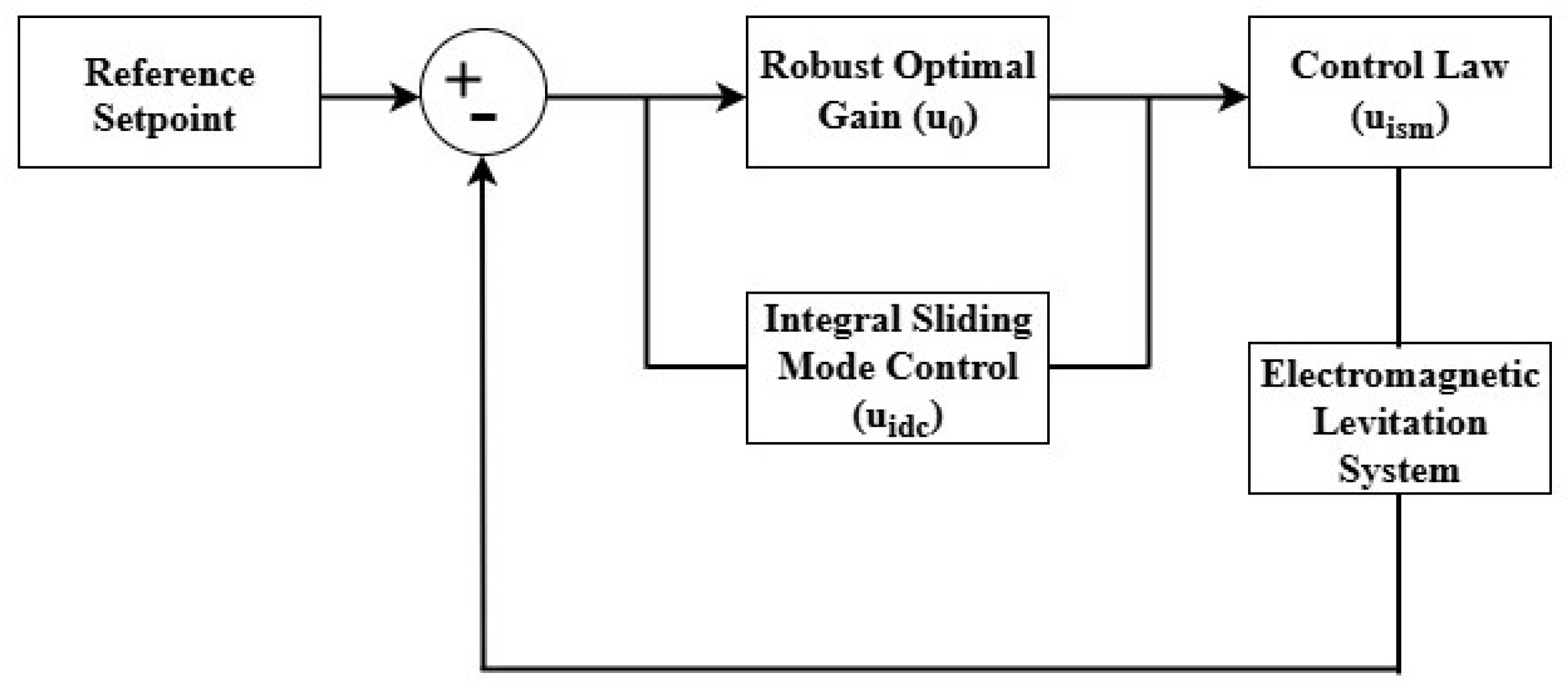
Therefore, the total control effort in the integral optimal sliding mode control can be written as shown in Equation (18). Figure 2 represents the schematic for the proposed control law.
u i s m = u 0 + u i d c
To ensure the optimality of the EMLS, the control effort u 0 is important; the control effort u 0 is a nominal controller, which is discussed in the next section of this article. Moreover, u i d c serves as a second control effort for the integral sliding mode control, which is known as the discontinuous control input. The discontinuous control mechanism is responsible for handling the system disturbances. This control effort helps the ISMC to achieve its set point efficiently. Equation (19) represents the integral sliding surface.
s i s m = N x ( t ) x ( 0 ) 0 t A x ( τ ) + g u 0 ( x , τ ) d τ
where N is selected such that the product of matrix N g must be invertible and the term N x ( 0 ) should ensure that the sliding surface is equal to zero such that it will eliminate the reaching phase. Therefore, the discontinuous control effort is highlighted by Equation (20).
u i d c = λ ( N g ) T s i s m ( N g ) T s i s m
where λ is a gain that guarantees the sliding phase motion. The uncertainty ω , which is Equation (17), is separated into two parts, i.e., matched and mismatched uncertainties, given by Equation (21).
ω = ω m + ω m m
where ω m is the matched component of uncertainties and ω m m is the mismatched component of uncertainties.
The matched component ω m = g g + ω and mismatched component ω m m = g g + ω , where g + is called the pseudo-inverse, which is used to decompose the uncertainties into matched and mismatched components, which are given as g + = ( g T g ) 1 g T , and g spans the null space of g + . Taking the derivative of Equation (19), we have
s ˙ i s m = N f + g ( u 0 + u i d c ) + g g + ω + g g + ω ( f + g u 0 )
Therefore, Equation (22) can be reframed as given in Equation (23)
s ˙ i s m = N g ( u i d c + g + ω ) + N ω m m
To prove the stability of the designed controller, consider the Lyapunov function
V = 1 2 s i s m 2
Equation (25) highlights the time derivate of the Lyapunov function
V ˙ = s i s m T N g λ ( N g ) T s i s m ( N g ) T s i s m + g + ω + N ω m m
V ˙ ( M g ) T s i s m ( λ g + ϕ ( M g ) 1 M ω m m )
Therefore, Equations (25) and (26) show that the system shown in Equation (17) is stable in the sense of Lyapunov [34]. The next part deals with the design of the nominal control law.

4.3. Optimal Control with Matched Uncertainties

The robust optimal framework with matched uncertainties is used to obtain the nominal control u n required in the integral optimal sliding mode control. The purpose of using this approach is to make the nominal control robust enough to provide better tracking of the desired values. In this section, the optimal gain is obtained for matched uncertainties [35].

Robust Optimal Control for Matched Uncertainty

Consider the nonlinear system shown in Equation (27)
x ˙ = ϕ ( x ) + ψ ( x ) u + ψ ( x ) Δ ( x )
where ψ ( x ) Δ ( x ) accounts for the system uncertainties. The matching condition is satisfied because the uncertainties lie in the range of ψ .
Assumption 3.
There exists a non-negative function such that the uncertainty Δ ( x ) is bounded, as shown in Equation (28)
Δ ( x ) Δ m a x ( x )
This assumption highlights the bounded uncertainty, which is a positive value. The control scheme u = K 1 ( x ) is to be obtained for the open-loop system shown in Equation (27) such that the closed-loop system shown in Equation (29) will remain globally asymptotically stable in the presence of uncertainties.
x ˙ = ϕ ( x ) + ψ ( x ) K 1 ( x ) + ψ ( x ) Δ ( x )
This robust issue is translated into an optimal control problem to calculate the feedback control law. For the nominal system, which is given by Equation (30)
x ˙ = ϕ ( x ) + ψ ( x ) u
the control scheme u = K 1 ( x ) will be obtained, which will be responsible for minimizing the cost function given by Equation (31)
0 ( Δ m a x ( x ) 2 + x T x + u T u ) d t
To relate the robust control problem to the optimal control problem, the following theorem is proposed.
Theorem 1.
If the solution to the optimal control problem discussed above exists, then the solution to the optimal control problem will become the solution to the robust control problem.
Proof. 
Assuming u = K 1 ( x ) is the solution to the optimal control problem discussed above, it has to be shown that Equation (32) is globally asymptotically stable in the presence of uncertainties.
x ˙ = ϕ ( x ) + ψ ( x ) K 1 ( x ) + ψ ( x ) Δ ( x )
Define a function V ( x 0 ) given by Equation (33) to be the minimum cost of the optimal control of the nominal system from some initial state x 0
V ( x 0 ) = m i n u R m 0 ( Δ m a x ( x ) 2 + x T x + u T u ) d t
The function V ( x ) is Lyapunov function for Equation (32) and it also satisfies the Hamilton–Jacobi–Bellman equation, which reduces to
m i n u R m ( Δ m a x ( x ) 2 + x T x + u T u + V x T ( ϕ ( x ) + ψ ( x ) u ) ) = 0
Since u = K 1 ( x ) is the optimal solution, it must satisfy the above equation, which is equal to
Δ m a x ( x ) 2 + x T x + K 1 ( x ) T K 1 ( x ) + V x T ( ϕ ( x ) + ψ ( x ) K 1 ( x ) ) = 0
Equation (35) can also be written as
V x T ( ϕ ( x ) + ψ ( x ) K 1 ( x ) ) = Δ m a x ( x ) 2 x T x K 1 ( x ) T K 1 ( x )
and
2 K 1 ( x ) T + V x T ψ ( x ) = 0
By minimizing the Hamiltonian of the system with respect to the control input u, the gain K 1 ( x ) is obtained. The minimization condition u of Equation (34) leads to the optimal control law shown in Equation (37), which minimizes the performance function 0 ( Δ m a x ( x ) 2 + x T x + u T u ) d t . The existence and uniqueness of the solution to the Hamilton–Jacobi–Bellman (HJB) equation are guaranteed since the cost functional is positive definite and the uncertainty term Δ ( x ) is bounded by a known positive function Δ m a x ( x ) . These conditions ensure that the function V ( x ) is continuously differentiable and positive definite.
With reference to equations above, it can be highlighted that V ( x ) is the Lyapunov function of Equation (32). Next, it will be shown that the time derivative of the Lyapunov function will remain negative. To prove this, consider Equation (38):
V ˙ ( x ) = V x T x ˙
Substituting x ˙ from Equation (32), Equation (38) can be reframed as shown in Equation (39):
V ˙ ( x ) = V x T ( ϕ ( x ) + ψ ( x ) K 1 ( x ) + ψ ( x ) Δ ( x ) )
The above equation can be rewritten as
V ˙ ( x ) = V x T ( ϕ ( x ) + ψ ( x ) K 1 ( x ) ) + V x T ( ψ ( x ) Δ ( x ) )
Using Equation (36) and (37) in Equation (40), we have
V ˙ ( x ) = Δ m a x ( x ) 2 x T x K 1 ( x ) T K 1 ( x ) 2 K 1 ( x ) T Δ ( x )
Adding and subtracting the term Δ ( x ) T Δ ( x ) in Equation (41), we obtain
V ˙ ( x ) = Δ m a x ( x ) 2 + Δ ( x ) T Δ ( x ) x T x K 1 ( x ) T K 1 ( x ) 2 K 1 ( x ) T Δ ( x ) Δ ( x ) T Δ ( x )
On rearranging Equation (42), we get
V ˙ ( x ) = Δ ( x ) 2 + Δ ( x ) T Δ ( x ) x T x ( K 1 ( x ) + Δ ( x ) ) T ( K 1 ( x ) + Δ ( x ) )
The term ( K 1 ( x ) + Δ ( x ) ) T ( K 1 ( x ) + Δ ( x ) ) is always positive; as a result ( K 1 ( x ) + Δ ( x ) ) T ( K 1 ( x ) + Δ ( x ) ) is always less than zero. Therefore, Equation (43) can be rewritten as
V ˙ ( x ) = Δ m a x ( x ) 2 + Δ ( x ) T Δ ( x ) x T x
Δ m a x ( x ) 2 > Δ ( x ) T Δ ( x ) ; as a result Δ m a x ( x ) 2 + Δ ( x ) T Δ ( x ) is always less than zero. Consequently, it could be said that
V ˙ ( x ) x T x
thereby confirming the global asymptotic stability of the closed-loop system under matched uncertainties. Thus, the EMLS will maintain stability when subjected to matched uncertainties in terms of the Lyapunov theorem. □

5. Results and Discussion

This section presents simulation results aimed at assessing the efficacy of the designed control strategy and providing insight into the design procedures for the EMLS. The numerical values for the EMLS have been selected as follows: The coil resistance is set at r c = 10 Ω , while the sensing resistance is r s = 1 Ω . The electromagnetic constant, which characterizes the interaction between the current in the coil and the magnetic field, is given by G e = 6.3508 × 10 5 N · m 2 A 2 . Additionally, the gravitational acceleration, g e , is valued at 9.81 m / s 2 . The mass of the object being levitated, referred to as the steel ball, is m b = 0.068 kg . The coil inductance, which affects how quickly the current can change in the coil, is defined as l c = 412.5 mH . Finally, the total travel distance of the steel object within the system is measured at T b = 0.014 m .
For the simulation, x 0 = [ 0.0125 m , 0 , 1.7856 A ] are the starting operating points for the position of the steel ball, velocity of the steel ball, and current flowing in the coil. The target position for the steel ball is determined to be x 1 d = 0.009 m . This desired position directly influences the current needed to achieve it, derived from the relationship defined by the equation x c = 2 g e × m b G e x a . The control input calculated as u = ( r c + r s ) x c .
To provide specific values, when the existing weight of the steel ball is m b = 68 gms , the resulting current is x c = 1.286 A and the corresponding control input is u = 14.146 Volts . If the mass experiences a 10% increase, bringing m b to 74.8 gms , the current adjusts to x c = 1.3491 A and the control input rises to u = 14.8401 Volts . In the case of a 20% increase in mass, where m b = 81.6 gms , the calculated values become x c = 1.4091 A and u = 15.5001 Volts . Lastly, for a 25% increase with m b = 85.2 gms , the current is x c = 1.4381 A and the control input is u = 15.73 Volts . These calculations illustrate how variations in mass influence the necessary electrical input for maintaining the desired position of the steel ball. The simulation experiments are carried out for two different controllers: one is for the SMC and the second is for IOSMC with matched uncertainties.
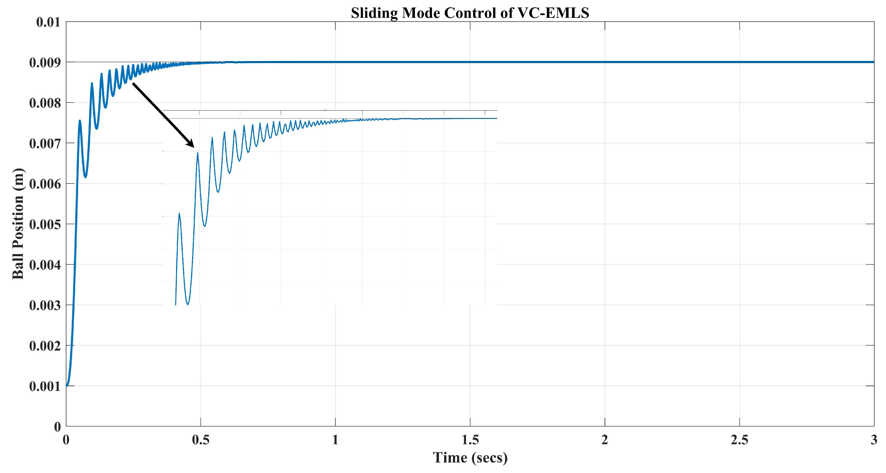
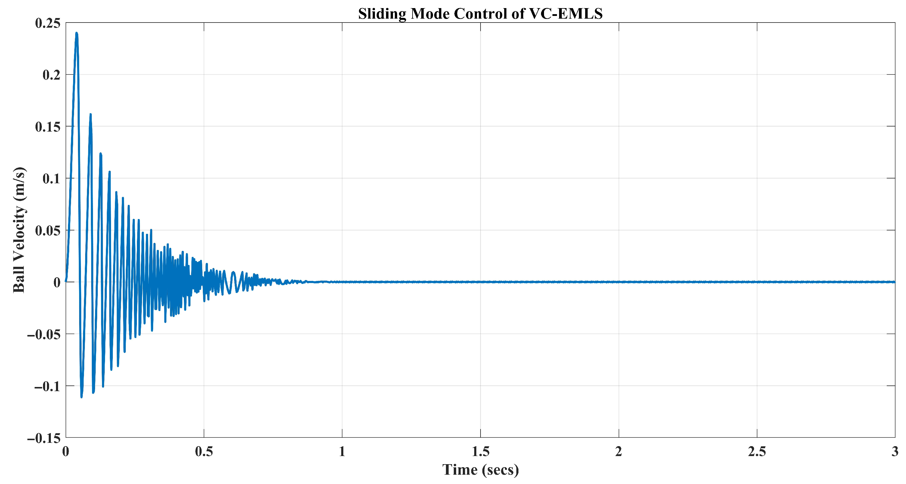
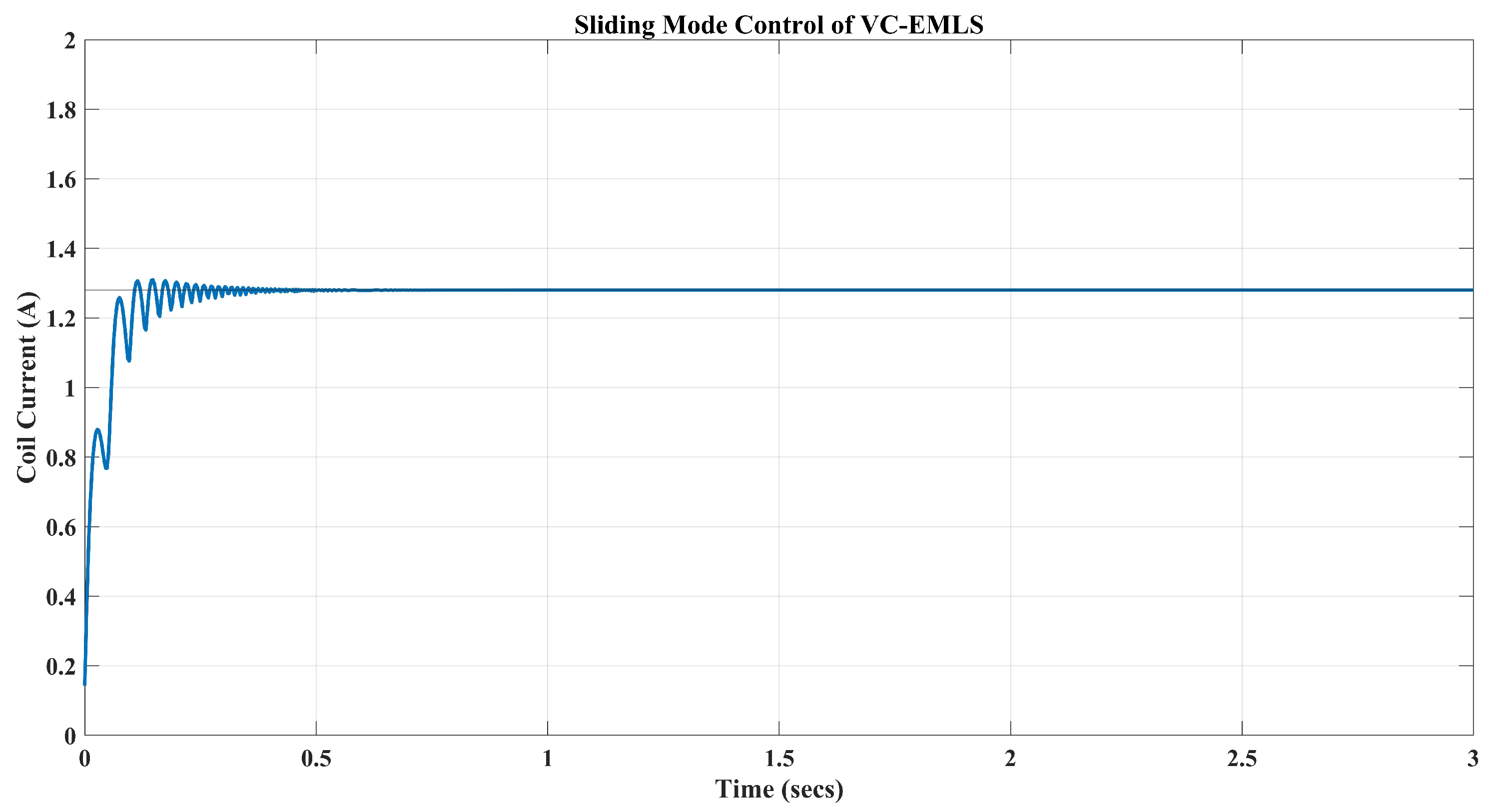
The parameter values used for the EMLS in SMC are illustrated above. The value of η = 0.5 is used in the simulation. N is calculated using the place command by placing the poles on the left-hand side of the s-plane. The values of A a a and A a b are selected from the linearized matrix A at the points x a 0 = 0.009 m and x c 0 = 1.2878 A . Figure 3 represents the position of the steel ball with the SMC technique; the tracking height of the steel ball is taken to be 9 mm . Figure 4 and Figure 5 showcase the velocity of the ball and current in the coil.
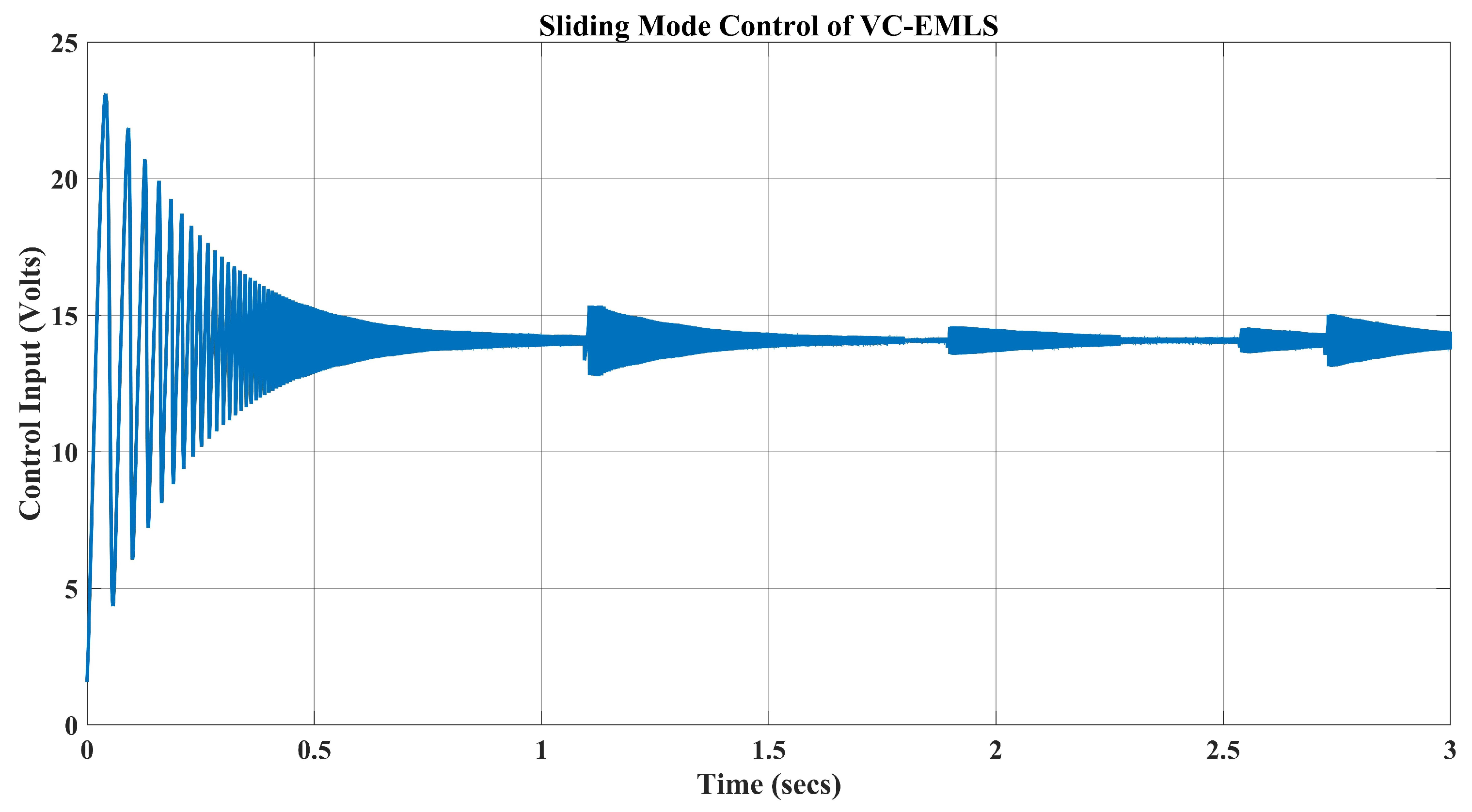
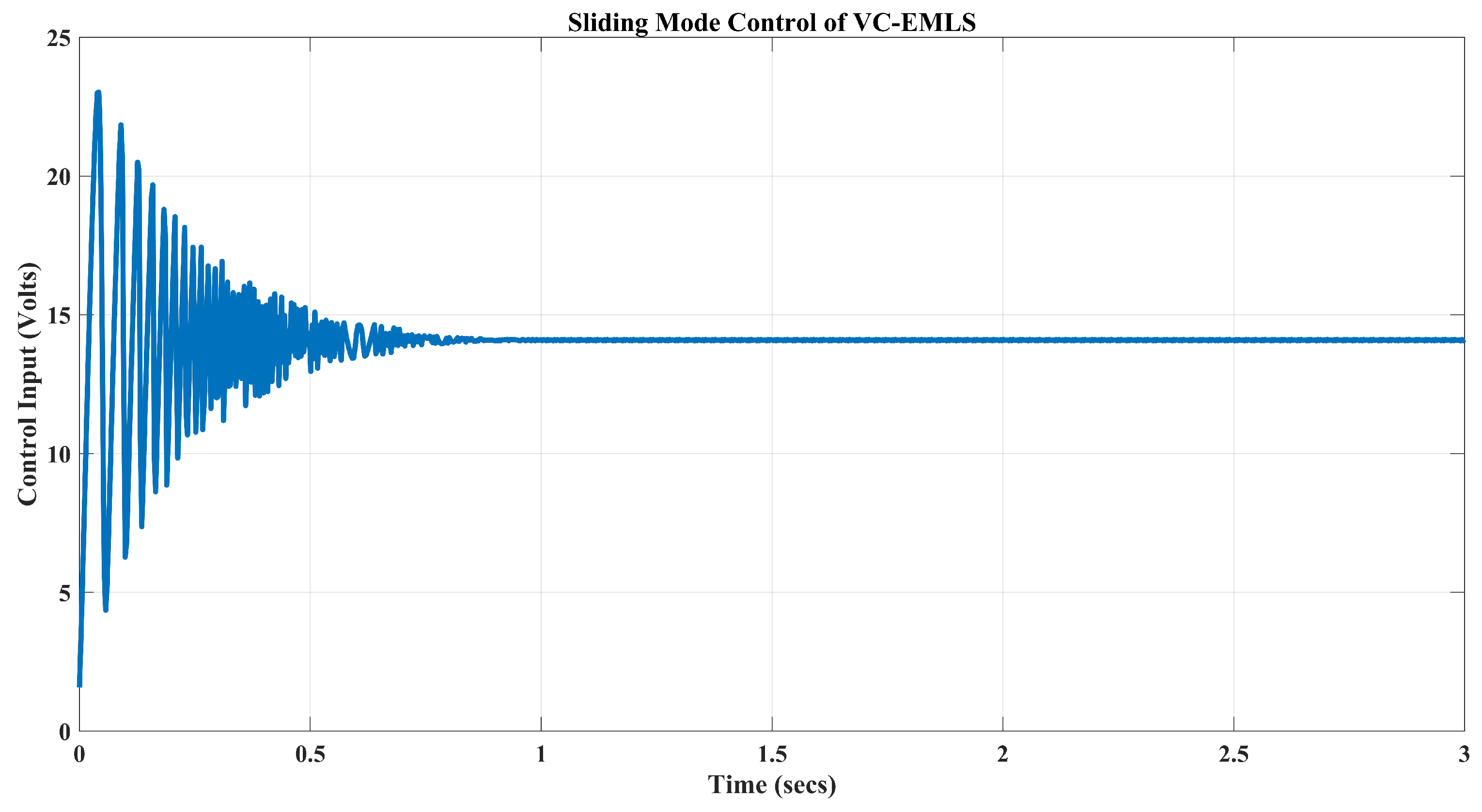
The figures show that there is an adequate amount of steady-state error between the desired position and the obtained result. Moreover, the variation present in the ball position and ball velocity is undesirable. The control input using the signum function is illustrated in Figure 6, and a substantial portion of high-frequency oscillations can be observed in the result. The control input using the tanh function is illustrated in Figure 7; a reduced chattering effect can be observed as compared to the signum function. However, a considerable amount of oscillations can still be observed in the result, which is one of the significant drawbacks of sliding mode control.
In this part, the discussion will focus on the simulation results of the control action provided by the robust integral optimal sliding mode control. While designing the control effort, as shown in Section 4.2, the IOSMC has two control actions: one is a discontinuous control action and the other is a nominal control action, which is provided by a robust optimal control scheme. Since the EMLS can suffer from parametric uncertainties, considering this condition of the system, uncertainties are considered for three cases while designing the optimal control action. These uncertainties account for the matched uncertainties; when the uncertainty can be separated from the system dynamics as a product of the input matrix, it is termed “matched uncertainty”. Hence, they are assumed as follows: the first uncertainty is assumed in the total resistance of the EMLS, i.e., r c + r s , the second is assumed only in the coil resistance r c , and the third is the in the sensing resistance r s . Using the controller design approach of Section 4.3, the controller gains are calculated for all the three uncertainties, which are [−15680 −296 77] for matched uncertainty in R c + R s , [−14828 −280 75] for matched uncertainty in R c , and [− 9240.9 −174.6 44.2] for matched uncertainty in R s .
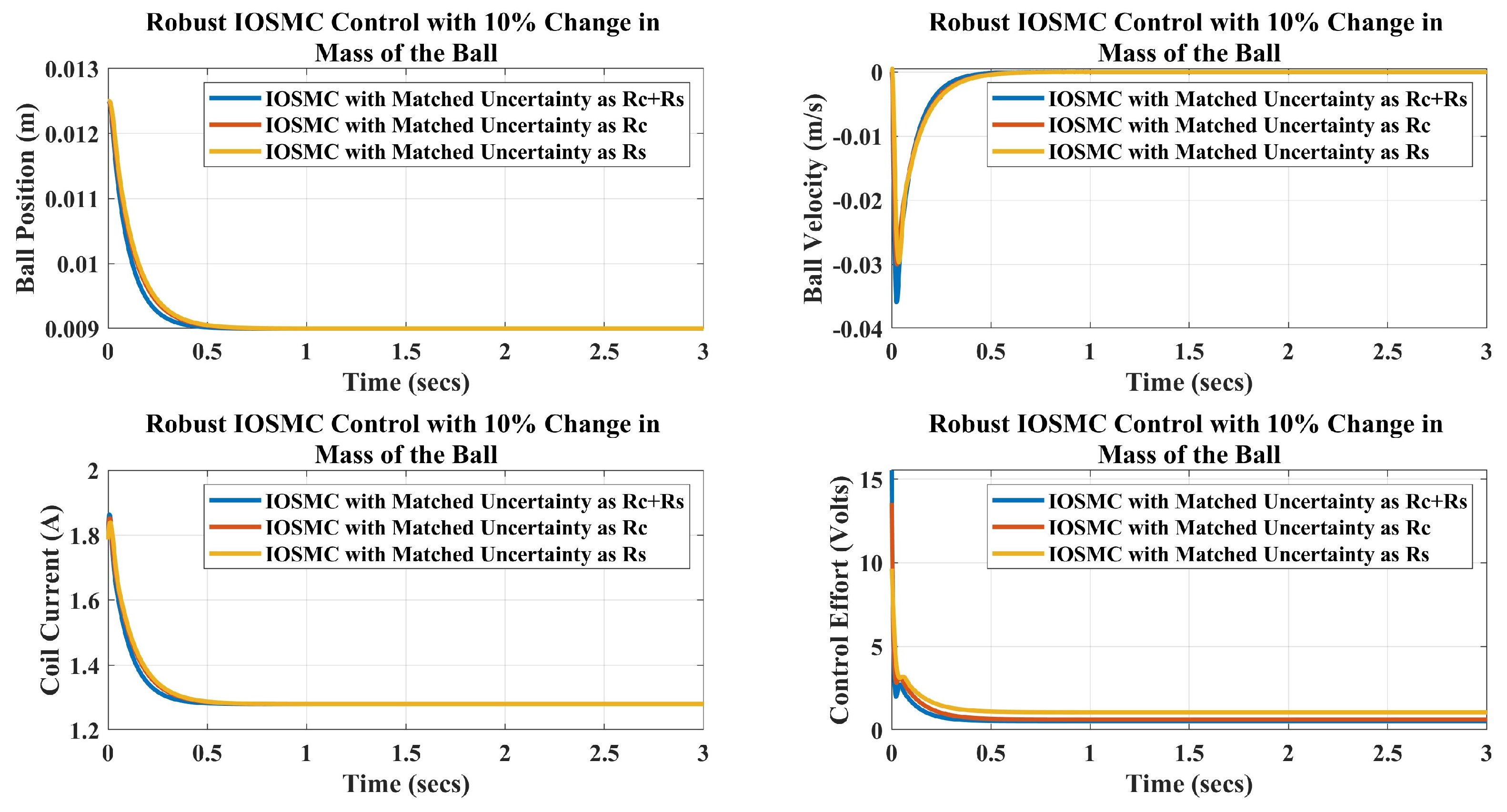
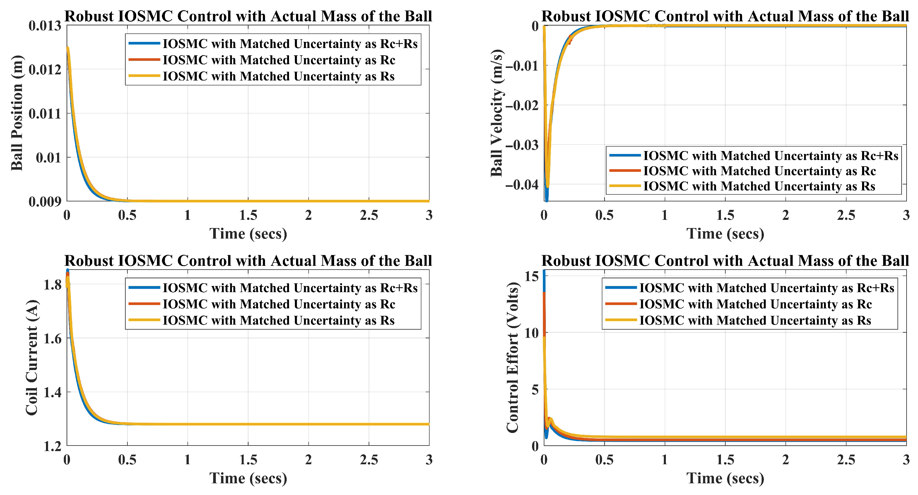
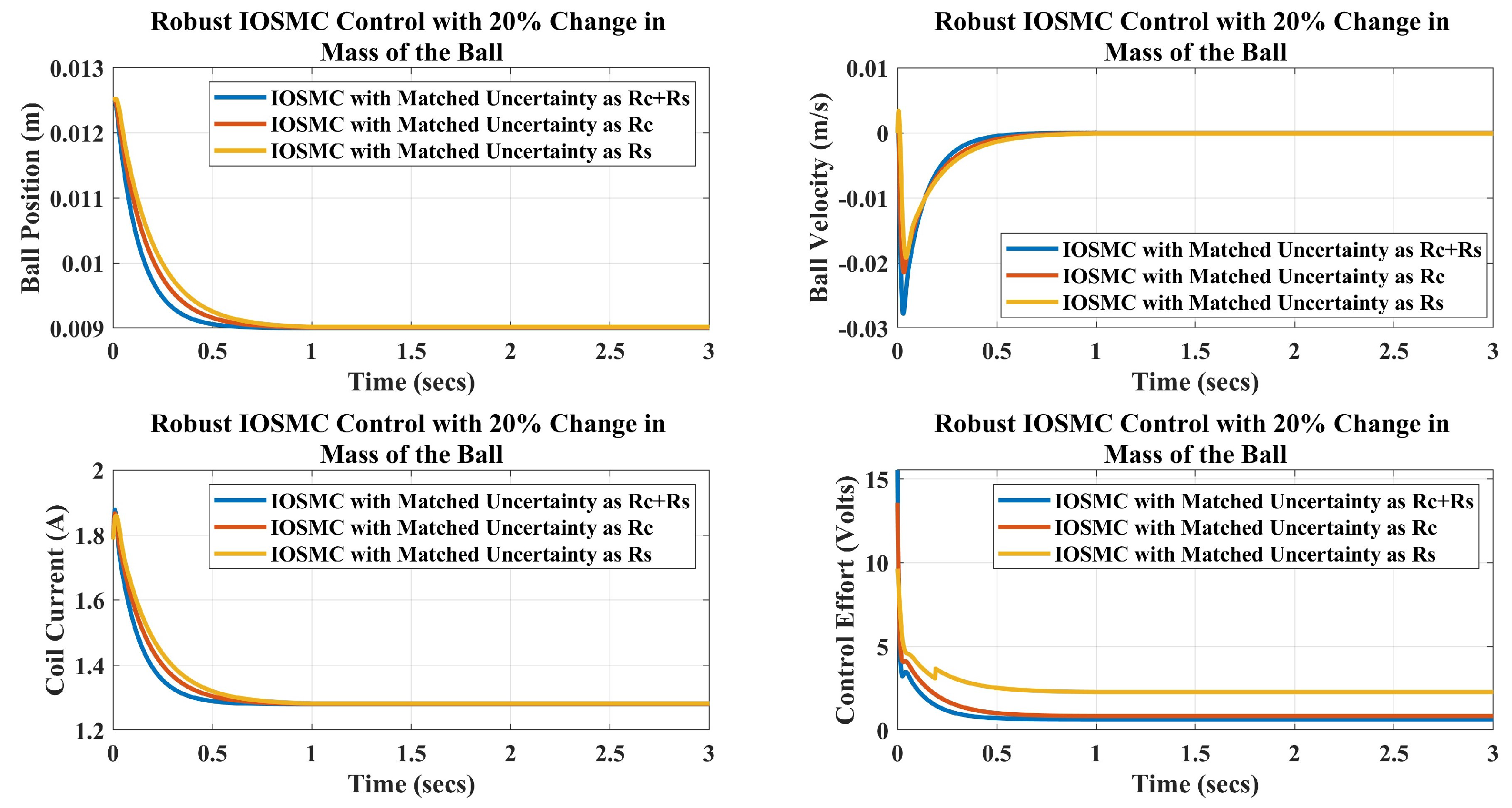
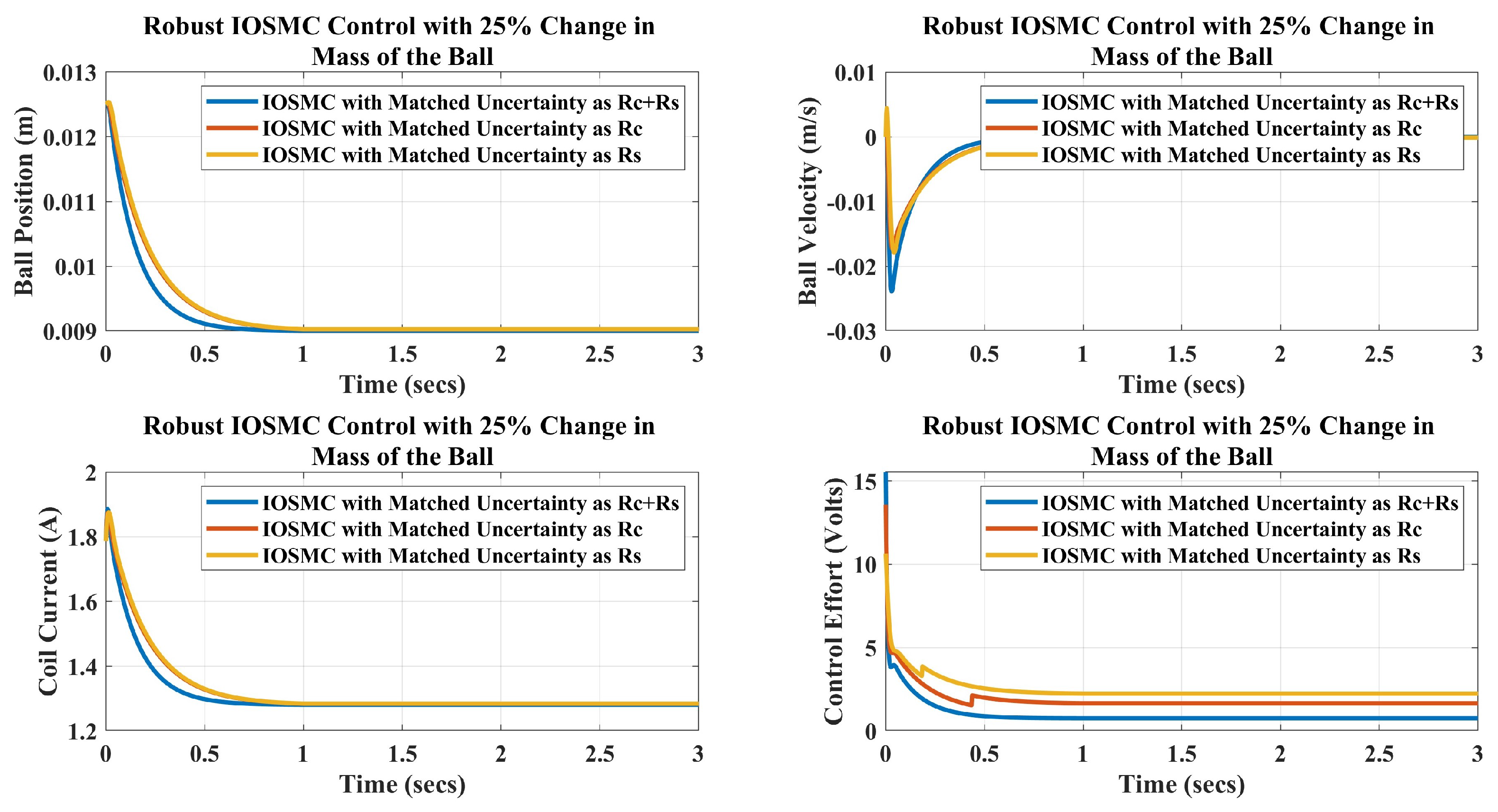
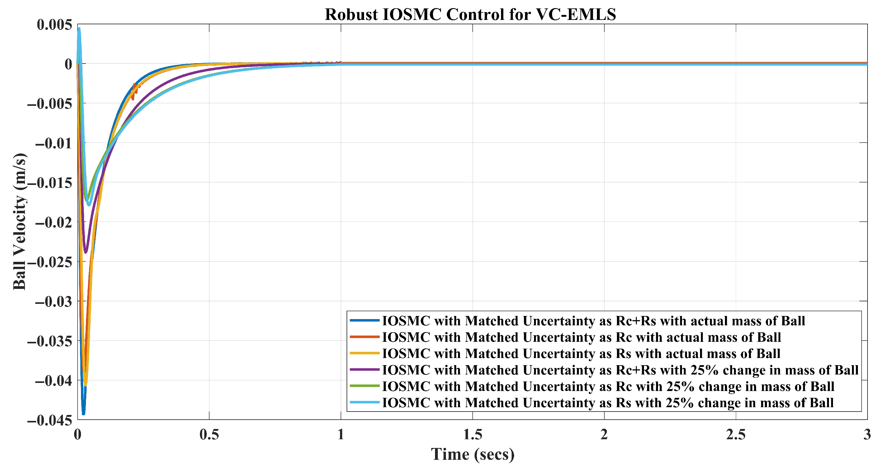
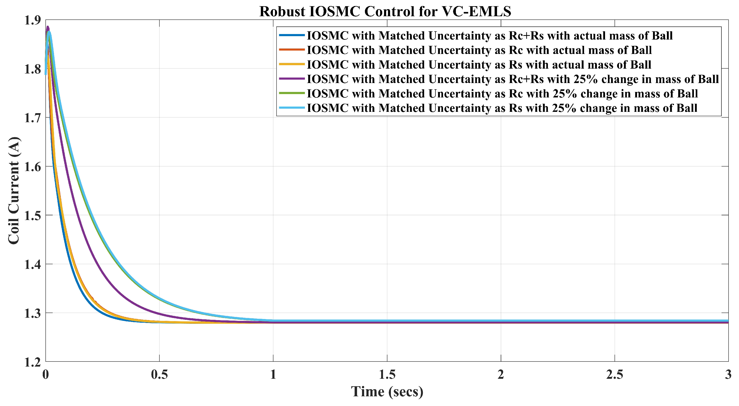
Figure 8, Figure 9, Figure 10 and Figure 11 show variations in the position of the steel ball, velocity of the steel ball, current in the coil, and control input with integral sliding mode control with robust optimal approaches for varying uncertainties along with the original weight of the steel ball and 10 % , 20 % , and 25 % changes in the weight of the ball. This comparison is drawn to highlight the efficiency of the designed control schemes when the system is subjected to a step disturbance in terms of the ball’s weight. From the figures, it is clear that the integral optimal control technique offers better robustness against parameter uncertainties compared to sliding mode control. Also, an oscillation-free control effort is obtained with the proposed control techniques.
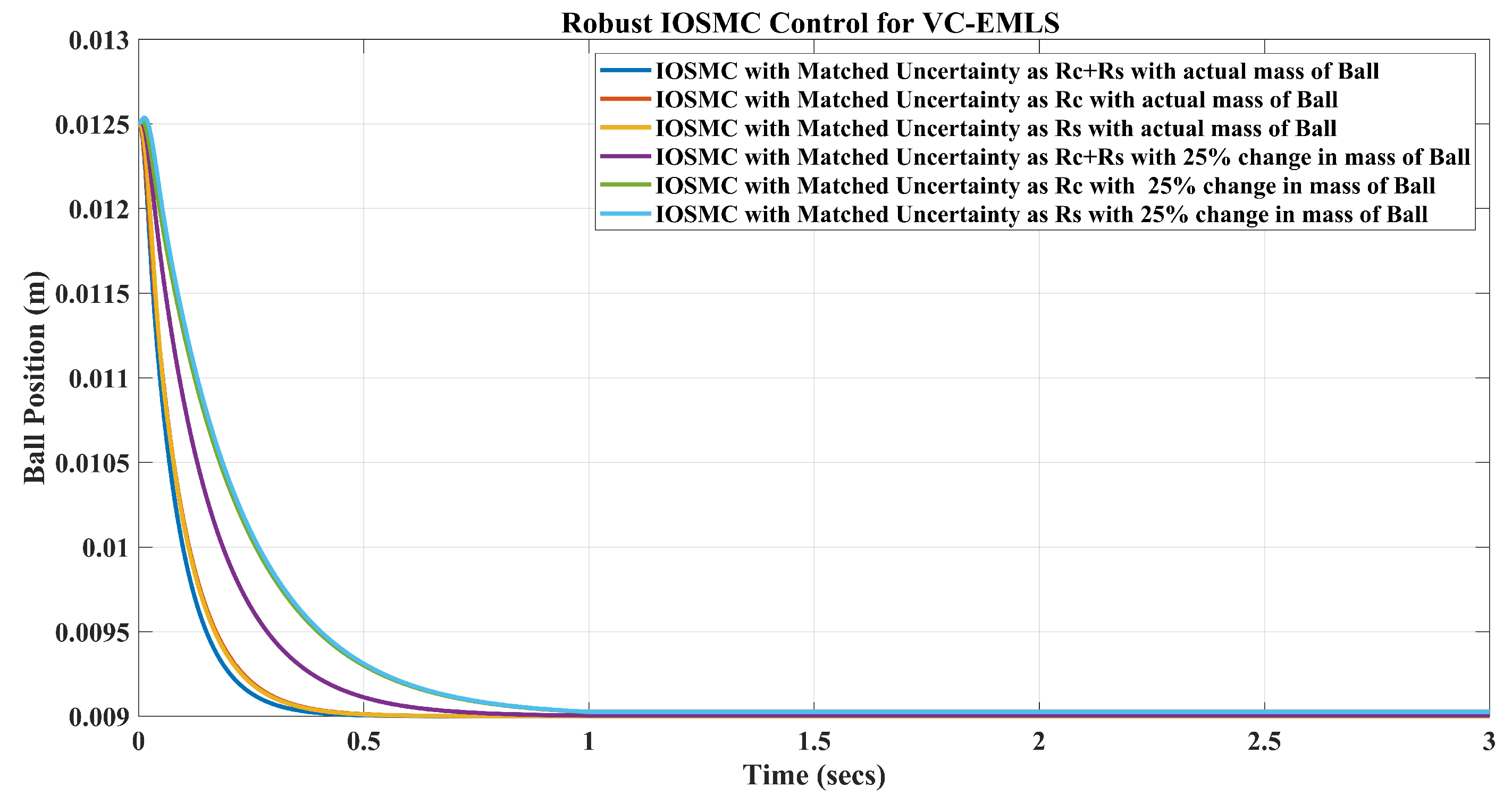
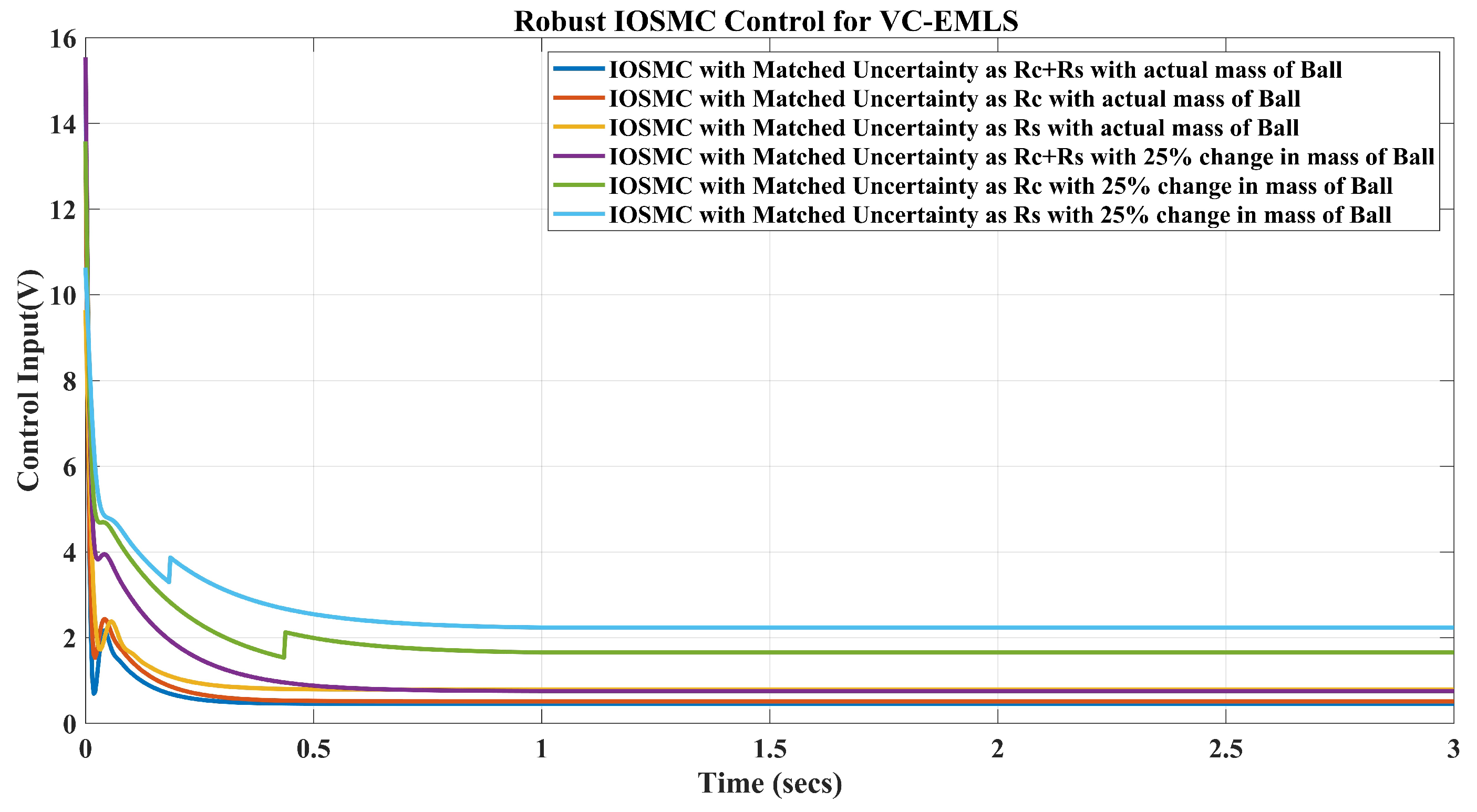
Figure 12, Figure 13, Figure 14 and Figure 15 show variations in the position of the steel ball, velocity of the steel ball, current in the coil, and control input with integral sliding mode control with different robust optimal approaches used to obtain the optimal gain with varying uncertainties along with the original weight of the steel ball and a 25 % change in the weight of the ball. From the figures, it is clear that the integral optimal control technique offers better robustness in terms of parameter uncertainty. This comparison is drawn to showcase the robustness of the proposed control technique when the EMLS is simulated with actual mass and with the highest change in mass of 25 % .
Figure 15 illustrates the control effort required by integral optimal sliding mode control with different uncertainties when the EMLS is simulated with the actual mass of the ball and a 25 % change in the ball mass. It is noted that the control effort requirement for the integral optimal sliding mode is much lower than that of the calculated value shown above. This is due to the fact that integral optimal sliding mode control involves three combinations of controllers: Sliding mode control, which offers robustness against uncertainties and disturbances due to its ability to force the states of the electromagnetic levitation system to follow the predefined sliding surface regardless of the uncertainties. Secondly, optimal control offers the minimization of the performance index, and by optimizing the control action, the IOSMC controller can achieve the desired control objective with minimal control effort. Lastly, the integral action helps to eliminate the steady-state error in achieving the desired set point. The integral action continuously integrates the tracking error over time and adjusts the control effort. As a result, IOSMC precisely achieves the desired set point of 9 mm without the need for excessive control effort, even in the presence of uncertainties.
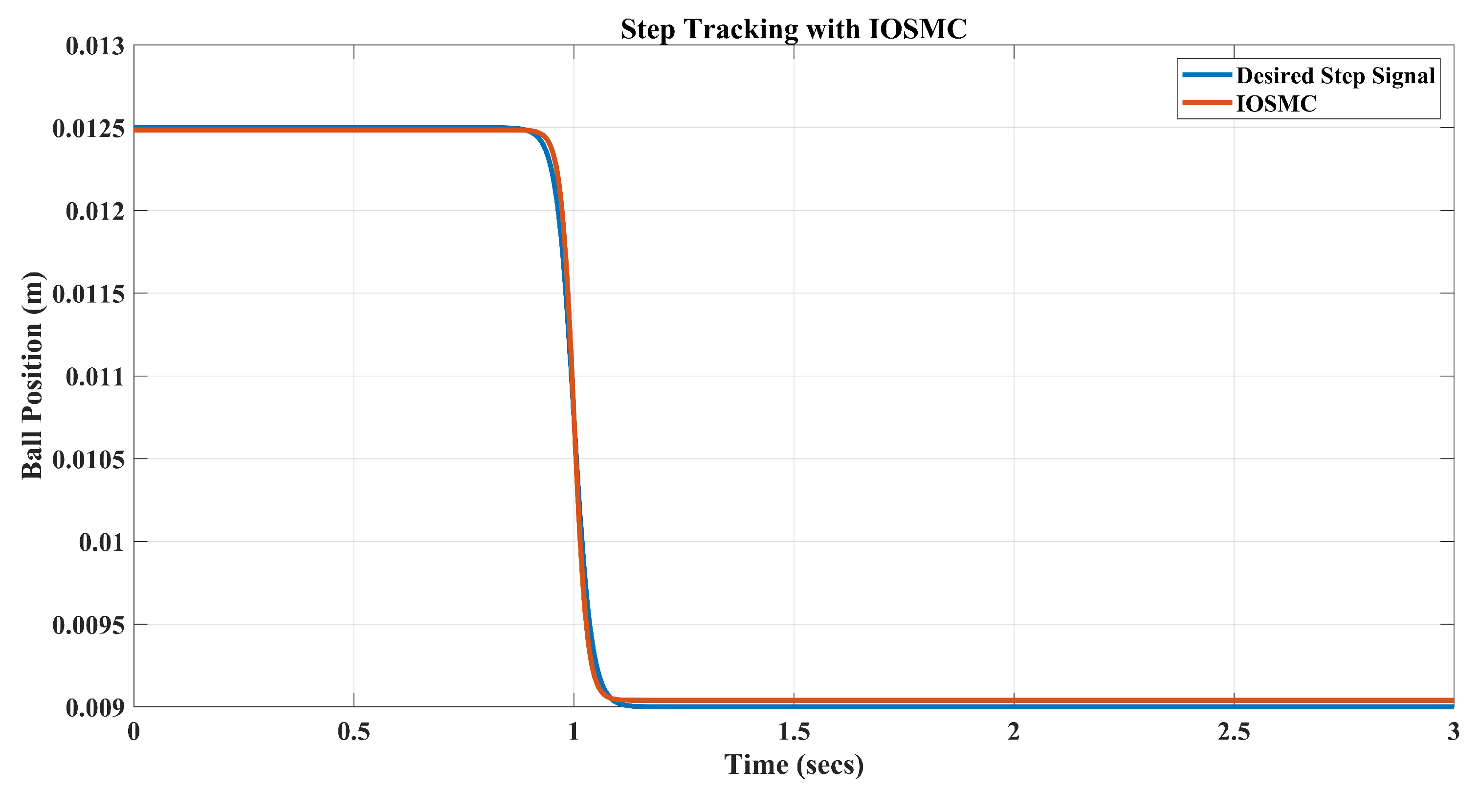
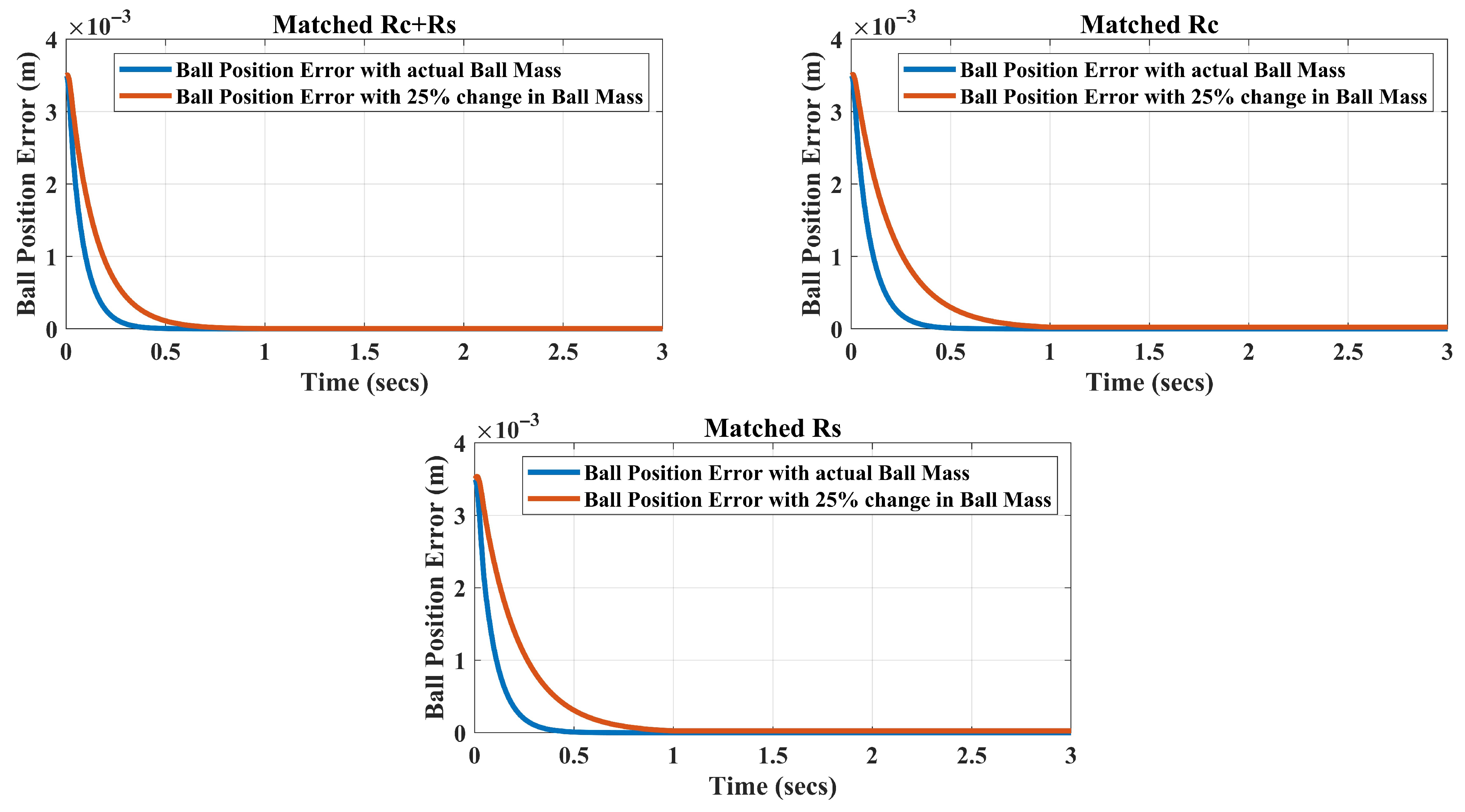
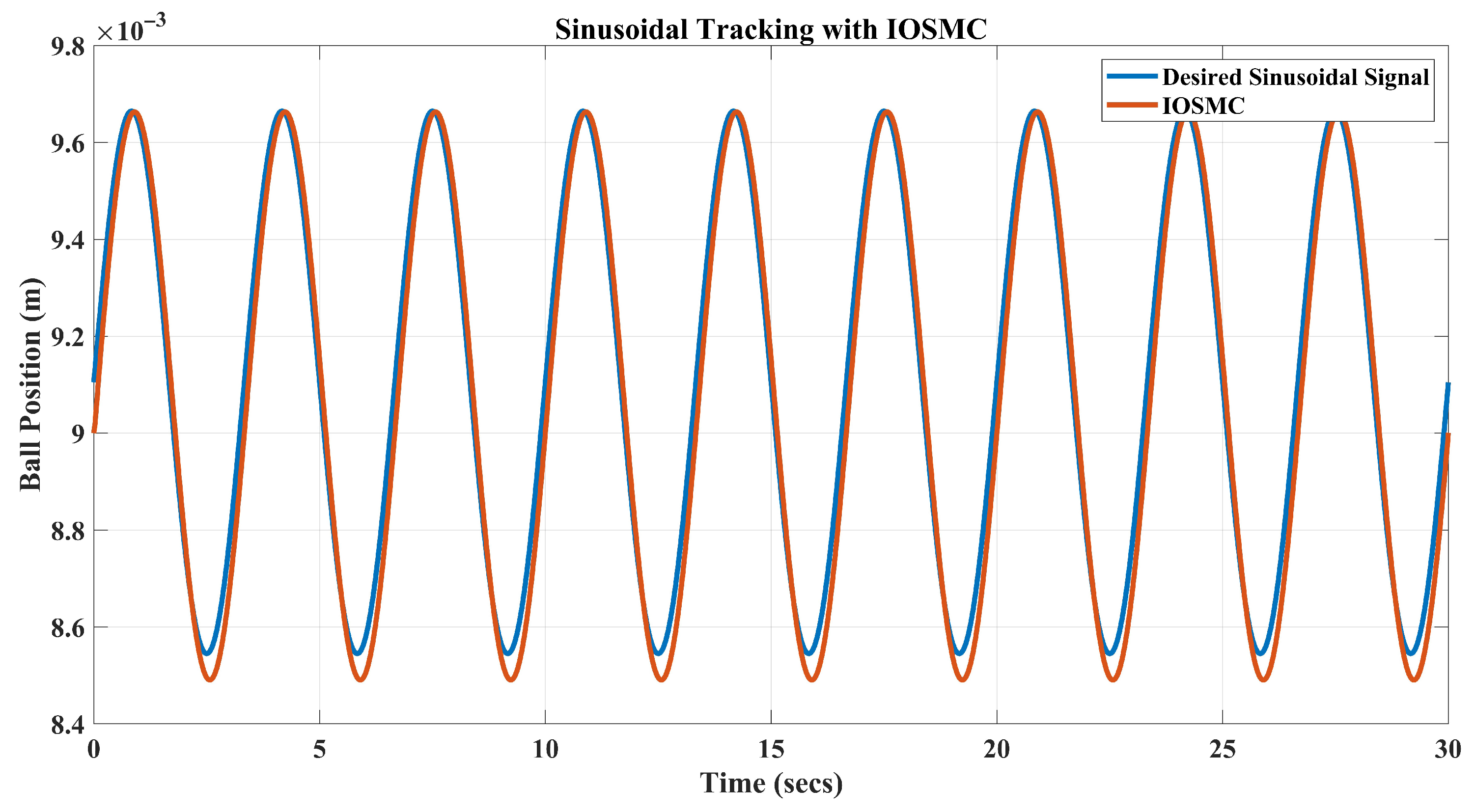
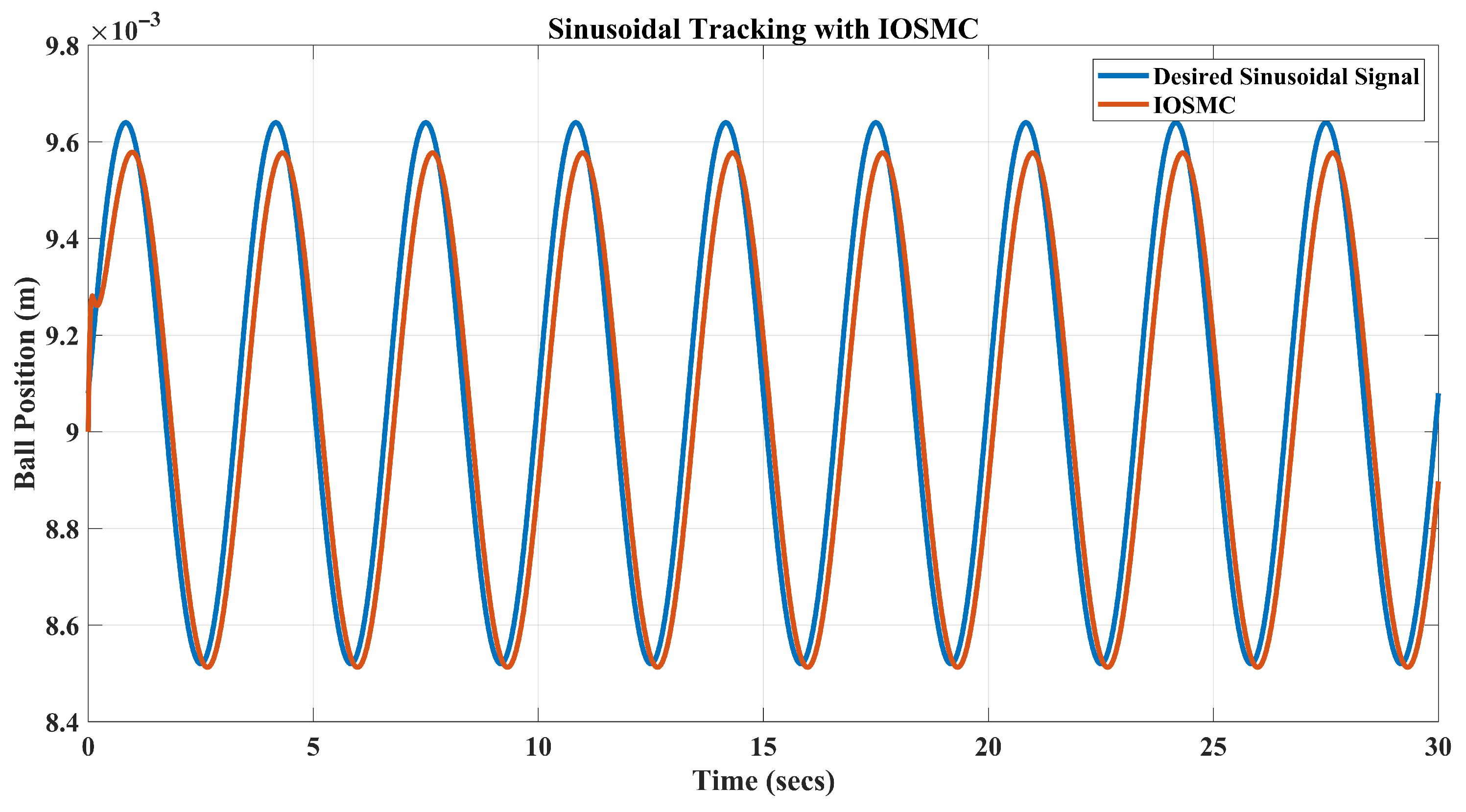
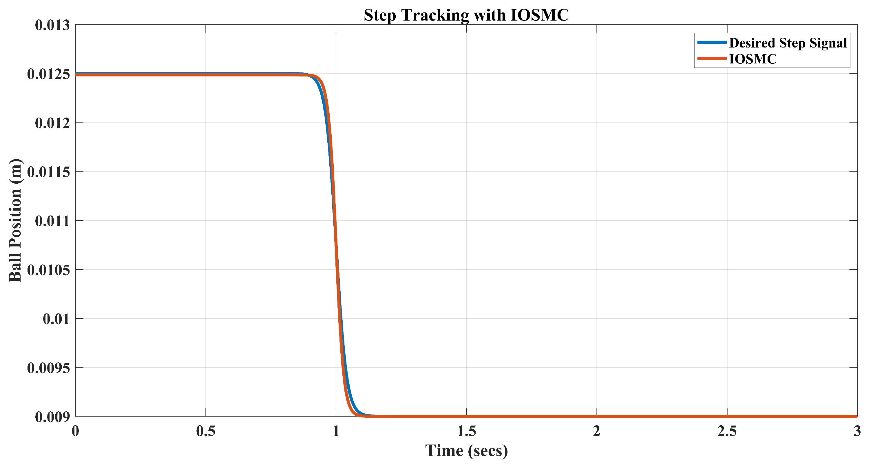
To provide further support for the proposed control strategy, the ball position error is plotted in Figure 16, along with the actual mass of the ball and a 25% change in the ball’s mass. The figure reveals that as soon as the ball attains the desired position, the error becomes zero for both cases, which highlights that IOSMC has no steady-state error and better robustness towards uncertainties compared to the sliding mode control. Additionally, the tracking situation cannot be limited to the desired set point alone; the tracking case can also be analyzed with various signals. Therefore, the sinusoidal tracking and step tracking are highlighted in Figure 17, Figure 18, Figure 19 and Figure 20, with the actual mass of the ball and a 25% change in the mass of the ball for the proposed control scheme. It is observed that the designed controller is capable of achieving the desired position with these signals. Hence, it proved that the proposed scheme is robust and efficient.
Table 1 and Table 2 present a comprehensive study of performance indices in terms of integral absolute error (IAE), integral square error (ISE), integral time absolute error (ITAE), and integral time square error (ITSE). This analysis is drawn when the EML system is subjected to a variation in the weight of the steel ball: one condition uses the actual mass of the steel ball and the other a 25 % change in the mass of the steel ball. It is evident from the table that when a disturbance of 25 % is applied to the system, the designed control strategy can handle this change, provided the optimal gain obtained from the matched uncertainty, considering the case of r c + r s , exhibits the best performance with negligible integral errors. To highlight the findings of the performance indices, the steel ball position error is also represented in Figure 16. The figure shows that the error in the position is almost negligible with the original weight of the steel ball, as well as when the mass of the ball is increased by 25 % . Furthermore, the control strategy designed by integrating the robust optimal gain and integral sliding mode control offers robustness. It enables the system to operate efficiently by maintaining the desired position of the ball in the presence of a disturbance.

6. Conclusions

This article designs a robust control scheme for a highly nonlinear and unstable electromagnetic levitation system. In the initial step, the mathematical and state-space equations of the EMLS are developed. The control strategy designed for the system is a combination of two robust controllers: sliding mode control with integral action and robust optimal control action. Since the sliding mode control mechanism has issues such as chattering and steady-state error, these problems can make the system unstable. Therefore, the integral action is added to overcome the disadvantage of the SMC. The robust optimal control action is added to the integral sliding mode control action to provide improved tracking of the desired set point. The robust optimal control action not only provides better tracking but also accounts for handling any kind of matched uncertainties in the system. The required feedback control gain is calculated by employing the HJB equation. The simulation results and performance index comparison highlight the efficiency and robustness of the designed control scheme. Comparative investigation of the performance indices proves that the proposed IOSMC attains, on average, a 45–60 % decrease in IAE and ITAE values compared with the traditional SMC technique, thereby confirming its higher robustness and tracking accuracy under parametric uncertainties. Forthcoming research will focus on the real-time hardware implementation of the proposed control strategy and the combination of metaheuristic optimization algorithms for adaptive tuning of the IOSMC gains, aiming to improve system performance in practical environments.

Author Contributions

Conceptualization, A.P., G.S., P.N.B. and R.K.; methodology, A.P.; validation, A.P.; formal analysis, A.P.; investigation, A.P., G.S. and R.K.; writing—original draft, A.P.; writing—review and editing, G.S., P.N.B. and R.K.; supervision, P.N.B. All authors have read and agreed to the published version of the manuscript.

Funding

This research received no external funding.

Data Availability Statement

The original contributions presented in this study are included in the article. Further inquiries can be directed to the corresponding author.

Conflicts of Interest

The authors declare no competing financial interests.

References

  1. Liu, J.J.; Chen, X.; Wang, J.M. Sliding mode control to stabilization of a tip-force destabilized shear beam subject to boundary control matched disturbance. J. Dyn. Control Syst. 2016, 22, 117–128. [Google Scholar] [CrossRef] [Scilit]
  2. Suárez-Cortez, R.; Alvarez-Gallegos, J.; González-Mora, E. Sliding controller design for a nonlinear fermentation system. Biotechnol. Bioeng. 1989, 33, 377–385. [Google Scholar] [CrossRef] [Scilit]
  3. Karunadasa, J.P.; Renfrew, A.C. Design and implementation of microporcessor based sliding mode controller for brushless servomotor. IEE Proc. B (Electric. Power Appl.) 1991, 138, 345–363. [Google Scholar] [CrossRef] [Scilit]
  4. Xu, J.X.; Guo, Z.Q.; Lee, T.H. Design and implementation of integral sliding-mode control on an underactuated two-wheeled mobile robot. IEEE Trans. Ind. Electron. 2013, 61, 3671–3681. [Google Scholar] [CrossRef] [Scilit]
  5. Unsal, C.; Kachroo, P. Sliding mode measurement feedback control for antilock braking systems. IEEE Trans. Control Syst. Technol. 2002, 7, 271–281. [Google Scholar] [CrossRef] [Scilit]
  6. Chen, Y.P.; Lo, S.C. Sliding-mode controller design for spacecraft attitude tracking maneuvers. IEEE Trans. Aerosp. Electron. Syst. 1993, 29, 1328–1333. [Google Scholar] [CrossRef] [Scilit]
  7. Cho, D.; Kato, Y.; Spilman, D. Sliding mode and classical controllers in magnetic levitation systems. IEEE Control Syst. Mag. 1993, 13, 42–48. [Google Scholar] [CrossRef] [Scilit]
  8. Chen, M.Y.; Wang, C.C.; Fu, L.C. Adaptive sliding mode controller design of a dual-axis maglev positioning system. In Proceedings of the 2001 American Control Conference. (Cat. No. 01CH37148), Arlington, VA, USA, 25–27 June 2001; Volume 5, pp. 3731–3736. [Google Scholar] [CrossRef] [Scilit]
  9. Bandal, V.S.; Vernekar, P.N. A new approach to a sliding mode controller design for a magnetic levitation system. In Proceedings of the 2009 Asia-Pacific Conference on Computational Intelligence and Industrial Applications (PACIIA), Wuhan, China, 28–29 November 2009; Volume 1, pp. 326–329. [Google Scholar] [CrossRef] [Scilit]
  10. Buckner, G.D. Intelligent bounds on modeling uncertainties: Applications to sliding mode control of a magnetic levitation system. In Proceedings of the 2001 IEEE International Conference on Systems, Man and Cybernetics. e-Systems and e-Man for Cybernetics in Cyberspace (Cat. No. 01CH37236), Tucson, AZ, USA, 7–10 October 2001; Volume 1, pp. 81–86. [Google Scholar] [CrossRef] [Scilit]
  11. Hassan, D.M.; Mohamed, A.M. Variable structure control of a magnetic levitation system. In Proceedings of the 2001 American Control Conference. (Cat. No. 01CH37148), Arlington, VA, USA, 25–27 June 2001; Volume 5, pp. 3725–3730. [Google Scholar] [CrossRef] [Scilit]
  12. Al-Muthairi, N.F.; Zribi, M. Sliding mode control of a magnetic levitation system. Math. Probl. Eng. 2004, 2004, 93–107. [Google Scholar] [CrossRef] [Scilit]
  13. Liu, C.; Zhang, J. Design of second-order sliding mode controller for electromagnetic levitation grip used in CNC. In Proceedings of the 2012 24th Chinese Control and Decision Conference (CCDC), Taiyuan, China, 23–25 May 2012; pp. 3282–3285. [Google Scholar] [CrossRef] [Scilit]
  14. Sathiyavathi, S. Design of sliding mode controller for magnetic levitation system. Comput. Electr. Eng. 2019, 78, 184–203. [Google Scholar] [CrossRef] [Scilit]
  15. Shou, B.; Zhang, H.; Long, Z.; Xie, Y.; Zhang, K.; Gu, Q. Design and applications of Q-learning adaptive PID algorithm for maglev train levitation control system. In Proceedings of the 2023 35th Chinese Control and Decision Conference (CCDC), Yichang, China, 20–22 May 2023; pp. 1947–1953. [Google Scholar] [CrossRef] [Scilit]
  16. Luo, Y.; Ni, F.; Lin, G.; Xu, J. Finite-time Control of High-speed Maglev Train Levitation System based on Terminal Sliding Mode. In Proceedings of the 2024 4th International Conference on Control Theory and Applications (ICoCTA), Hangzhou, China, 18–20 October 2024; pp. 186–190. [Google Scholar] [CrossRef] [Scilit]
  17. Wen, J.; Wu, J.; Tian, Y. Levitation control of maglev systems based on cascade control. In Proceedings of the 2022 China Automation Congress (CAC), Xiamen, China, 25–27 November 2022; pp. 4311–4315. [Google Scholar] [CrossRef] [Scilit]
  18. Teklu, E.A.; Abdissa, C.M. Genetic algorithm tuned super twisting sliding mode controller for suspension of maglev train with flexible track. IEEE Access 2023, 11, 30955–30969. [Google Scholar] [CrossRef] [Scilit]
  19. Sharma, A.; Amrr, S.M.; Nabi, M.; Banerjee, S. Extended state observer based integral sliding mode control of maglev systems with enhanced chattering alleviation. In Proceedings of the 2021 Seventh Indian Control Conference (ICC), Mumbai, India, 20–22 December 2021; pp. 242–247. [Google Scholar] [CrossRef] [Scilit]
  20. Nguyen, V.-T.; Pham, D.-H.; Mai, V.T.; Nguyen, H.-N.; Phan, M.-T. Design of Intelligent Control Using Dynamic Petri, CMAC, and BCMO for Nonlinear Systems with Uncertainties. Mathematics 2025, 13, 2825. [Google Scholar] [CrossRef] [Scilit]
  21. Aliasghary, M.; Jalilv, A.; Teshnehlab, M.; Shoorehdeli, M.A. Sliding mode control of magnetic levitation system using radial basis function neural networks. In Proceedings of the 2008 IEEE Conference on Robotics, Automation and Mechatronics, Chengdu, China, 21–24 September 2008; pp. 467–470. [Google Scholar] [CrossRef] [Scilit]
  22. Zhang, Z.; Zhou, Y.; Tao, X. Model predictive control of a magnetic levitation system using two-level state feedback. Meas. Control 2020, 53, 962–970. [Google Scholar] [CrossRef] [Scilit]
  23. Alkurawy, L.J.; Mohammed, K.G. Mohammed. Model predictive control of magnetic levitation system. Int. J. Electr. Comput. Eng. (IJECE) 2020, 10, 5802. [Google Scholar] [CrossRef] [Scilit]
  24. Peng, T.; Li, H.; Peng, H.; Tian, X.; Qin, Y.; Peng, X. A novel nonlinear model predictive control strategy and its application to maglev ball system. Int. J. Control 2025, 98, 782–795. [Google Scholar] [CrossRef] [Scilit]
  25. Liu, Z.; Dou, F. Linear Model Predictive Control and Back-Propagation Controller for Single-Point Magnetic Levitation with Different Gap Levitation and Back-Propagation Offline Iteration. Actuators 2024, 13, 331. [Google Scholar] [CrossRef] [Scilit]
  26. Ke, Z.; Yi, H.; Zhang, P.; Feng, Y.; Liang, L.; Deng, Z. Model predictive control based on Q-learning for magnetic levitation platform system. Int. J. Appl. Electromagn. Mech. 2024, 76, 289–305. [Google Scholar] [CrossRef] [Scilit]
  27. Wu, Z.; Fan, K.; Zhang, X.; Li, W. Based on sliding mode and adaptive linear active disturbance rejection control for a magnetic levitation system. J. Sens. 2023, 2023, 5568976. [Google Scholar] [CrossRef] [Scilit]
  28. Boonsatit, N.; Pukdeboon, C. Adaptive fast terminal sliding mode control of magnetic levitation system. J. Control Autom. Electr. Syst. 2016, 27, 359–367. [Google Scholar] [CrossRef] [Scilit]
  29. Lu, Y.; Lu, J.; Tan, C.; Tian, M.; Dong, G. Adaptive non-singular terminal sliding mode control method for electromagnetic linear actuator. Micromachines 2022, 13, 1294. [Google Scholar] [CrossRef] [Scilit] [PubMed]
  30. Khaniki, M.S.; Khosrowjerdi, M.J. An optimal integral sliding mode control using multiobjective H2/H approach to surface design. In Proceedings of the 2010 18th Iranian Conference on Electrical Engineering, Isfahan, Iran, 11–13 May 2010; pp. 698–703. [Google Scholar] [CrossRef] [Scilit]
  31. Haiping, P.; Xia, C. Global robust optimal sliding mode control for uncertain affine nonlinear systems. J. Syst. Eng. Electron. 2009, 20, 838–843. [Google Scholar]
  32. Liu, R.; Li, S. Optimal integral sliding mode control scheme based on pseudospectral method for robotic manipulators. Int. J. Control 2014, 87, 1131–1140. [Google Scholar] [CrossRef] [Scilit]
  33. Pandey, A.; Adhyaru, D.M. Robust–optimal control of electromagnetic levitation system with matched and unmatched uncertainties: Experimental validation. Control Theory Technol. 2025, 23, 28–48. [Google Scholar] [CrossRef] [Scilit]
  34. Jose, J.; Mija, S.J. An output feedback integral optimal sliding mode controller for magnetic levitation systems. In Proceedings of the 2020 Fourth International Conference on Inventive Systems and Control (ICISC), Coimbatore, India, 8–10 January 2020; pp. 197–202. [Google Scholar] [CrossRef] [Scilit]
  35. Adhyaru, D.M.; Kar, I.N.; Gopal, M. Fixed final time optimal control approach for bounded robust controller design using Hamilton–Jacobi–Bellman solution. IET Control Theory Appl. 2009, 3, 1183–1195. [Google Scholar] [CrossRef] [Scilit]
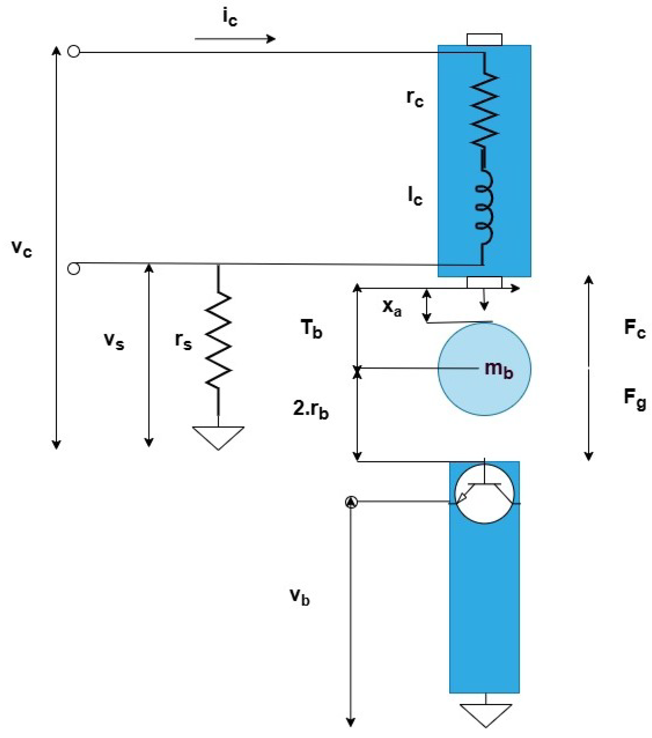
Figure 1. Structure of EMLS.
Mathematics 14 00229 g001
Figure 2. Schematic for integral optimal sliding mode control.
Mathematics 14 00229 g002
Figure 3. Ball position (m).
Mathematics 14 00229 g003
Figure 4. Ball velocity (m/s).
Mathematics 14 00229 g004
Figure 5. Coil current (A).
Mathematics 14 00229 g005
Figure 6. Control input (volts).
Mathematics 14 00229 g006
Figure 7. Control input (volts) with tanh.
Mathematics 14 00229 g007
Figure 8. Position, velocity, coil current, and control input for actual mass with IOSMC.
Mathematics 14 00229 g008
Figure 9. Position, velocity, coil current, and control input for 10 % change in mass with IOSMC.
Mathematics 14 00229 g009
Figure 10. Position, velocity, coil current, and control input for 20 % change in mass with IOSMC.
Mathematics 14 00229 g010
Figure 11. Position, velocity, coil current, and control input for 25 % change in mass with IOSMC.
Mathematics 14 00229 g011
Figure 12. Ball position (m) with IOSMC.
Mathematics 14 00229 g012
Figure 13. Ball velocity (m/s) with IOSMC.
Mathematics 14 00229 g013
Figure 14. Coil current (A) with IOSMC.
Mathematics 14 00229 g014
Figure 15. Coil voltage (volts) with IOSMC.
Mathematics 14 00229 g015
Figure 16. Ball position error (m).
Mathematics 14 00229 g016
Figure 17. Sinusoidal tracking of ball position (m) with actual mass.
Mathematics 14 00229 g017
Figure 18. Sinusoidal tracking of ball position (m) with 10% change in mass.
Mathematics 14 00229 g018
Figure 19. Step tracking of ball position (m) with actual mass.
Mathematics 14 00229 g019
Figure 20. Step tracking of ball position (m) with 10% change in mass.
Mathematics 14 00229 g020
Table 1. Integral error comparison with actual mass.
ControllersIAEISEITAEITSE
SMC-Signum Function 5.6030 × 10 4 2.1266 × 10 6 1.0482 × 10 4 6.7085 × 10 8
SMC-tanh Function 5.1378 × 10 4 2.1008 × 10 6 3.8211 × 10 5 6.1363 × 10 8
IOSMC-Matched ( R c + R s ) 2.8340 × 10 4 5.4041 × 10 7 2.1218 × 10 5 1.9996 × 10 8
IOSMC-Matched ( R c ) 3.2253 × 10 4 6.1098 × 10 7 2.7764 × 10 5 2.5886 × 10 8
IOSMC-Matched ( R s ) 3.2696 × 10 4 6.2036 × 10 7 2.7973 × 10 5 2.5964 × 10 8
Table 2. Integral error comparison with 25 % change in mass.
ControllersIAEISEITAEITSE
SMC-Signum Function 2.8589 × 10 2 2.3266 × 10 6 6.8266 × 10 4 3.8302 × 10 7
SMC-tanh Function 2.5215 × 10 2 2.1225 × 10 6 6.5776 × 10 4 3.2991 × 10 7
IOSMC-Matched ( R c + R s ) 5.4204 × 10 4 1.0156 × 10 6 8.9123 × 10 5 7.1732 × 10 8
IOSMC-Matched ( R c ) 7.8702 × 10 4 1.3944 × 10 6 2.4016 × 10 4 1.4011 × 10 7
IOSMC-Matched ( R s ) 1.20236 × 10 2 1.9589 × 10 6 5.8496 × 10 4 2.8548 × 10 7
Disclaimer/Publisher’s Note: The statements, opinions and data contained in all publications are solely those of the individual author(s) and contributor(s) and not of MDPI and/or the editor(s). MDPI and/or the editor(s) disclaim responsibility for any injury to people or property resulting from any ideas, methods, instructions or products referred to in the content.