Abstract
This paper presents a novel dynamic adaptive event-triggered mechanism (DAETM) for addressing actuator saturation in leader–follower fractional-order nonlinear multi-agent networked systems (FONMANSs). By utilizing a sector-bounded condition approach and a convex hull representation technique, the proposed method effectively addresses the effects of actuator saturation. This results in less conservative linear matrix inequality (LMI) criteria, guaranteeing asymptotic consensus among agents within the FONMANS framework. The proposed sufficient conditions are computationally efficient, requiring only simple LMI solutions. The effectiveness of the approach is validated through practical applications, such as synchronous generators within a FONMANS framework, where it demonstrates superior performance and robustness. Additionally, comparative studies with Chua’s circuit system enhance the robustness and efficiency of control systems compared to existing techniques. These findings highlight the method’s potential for broad application across various multi-agent systems, particularly in scenarios with limited communication and actuator constraints. The proposed approach enhances system performance and provides a robust, adaptive control solution for dynamic and uncertain environments.
Keywords:
fractional order; multi-agent systems; event-triggered mechanism; actuator saturation; synchronous generators MSC:
93A16; 93D50; 93B70; 26A33
1. Introduction
A significant area of research in multi-agent systems (MASs) is mainly focused on integer-order systems. However, specific scenarios such as vehicles moving through muddy terrain or drones operating in challenging weather conditions such as rain or snow may endanger system stability depending on integer-order models. In these instances, fractional-order systems offer a more advantageous solution. For example, ref. [1] investigated an adaptive event-triggered (ET) stochastic estimator-based sampled-data controller to ensure bounded mean-square stability in a fractional-order PMSG-based wind energy system. Similarly, ref. [2] proposed a fuzzy memory-based fault-tolerant control framework with external disturbances and maintained stability in a fractional-order nonlinear PMSG model. Fractional-order systems are more adept at modeling the actual physical characteristics of objects and have wide-ranging practical applications [3]. Consequently, growing interest has been in addressing the leader–follower consensus control challenges in fractional-order MASs (FOMASs). For instance, ref. [4] investigated the consensus problem in FOMASs through observer-based boundary value control. The cybersecure consensus issue in FOMASs with distributed delays and DoS attacks was explored in [5]. The fault-tolerant consensus problem for heterogeneous FOMASs with uncertain nonlinearities was analyzed in [6], while [7] focused on containment control in discrete-time FOMASs with input delays. Moreover, ref. [8] addressed the leader–following consensus challenge in FOMASs using output feedback.
To address the challenge of limited resources, recent research has proposed sampled-data control, where agents update their data at predetermined intervals [9,10,11]. However, this approach often requires a conservative sampling period to maintain consensus in FOMASs, leading to unnecessary energy consumption. For example, ref. [12] investigated an ET sampled-data control method for FOMASs that relies on global information and assumes an undirected communication topology. On the other hand, ref. [13] proposed a distributed ET control method for linear FOMASs under directed graphs, although its time-dependent exponential threshold may not fully capture dynamic changes in the system. In [14], a state-dependent triggering function based on neighborhood information was explored; this method continues to demand constant communication, limiting its efficiency. In contrast, dynamic ET mechanisms, which involve non-negative variables, provide significant improvements in resource efficiency, as demonstrated by recent research [15,16,17,18,19,20]. This insight, combined with adaptive controllers that adjust parameters based on dynamic rules, inspired the development of the DAETC mechanism for FOMASs, offering a novel approach to consensus control with enhanced resource utilization.
Although DAETC is mainly focused on enhancing control inputs, actuator saturation remains a significant practical challenge related to control inputs. For example, ref. [21] studied the ET consensus of matrix-weighted networks under actuator saturation, while [22] investigated neural-based formation control in uncertain MASs with actuator saturation. Similarly, ref. [23] analyzed the robustness of MASs under actuator faults and saturation, concentrating on consensus control. However, none of these studies address FONMANS, which forms the foundation of our research. Therefore, this paper extends existing methods by applying the DAETC mechanism to FONMANS, in which both actuator saturation and ET behaviors are essential in maintaining system stability and performance. The proposed approach offers a more energy-efficient and robust strategy for consensus control in sophisticated, resource-limited systems.
Based on the above discussion, this study investigates the issue of leader–follower FONMANS with actuator saturation and general nonlinear dynamics using the DAETM. The main contributions of this paper are as follows:
- 1.
- We developed a DAETM scheme to address leader–follower FONMANS with actuator saturation, achieving asymptotic stability using Mittag–Leffler functions.
- 2.
- This study proposes two strategies, namely the sector-bounded and convex hull methods, that effectively tackle actuator saturation, reduce conservatism, and enhance system flexibility using fractional Lyapunov functions and LMIs.
- 3.
- The proposed controller is validated through simulations using a synchronous generator (SG) model and comparative studies with the Chua circuit system, demonstrating the superior performance of the DAETM approach.
2. Preliminaries
2.1. Algebraic Graph Theory
The collaborative behavior of agents in MASs depends significantly on the structure of the communication network between the agents. A directed graph, denoted by G, is often used to show the interactions and the flow of information among agents. Specifically, is a weighted directed graph, where represents the set of nodes corresponding to the M agents in the system, and represents the directed edges that indicate the communication links between these agents. The edge in the graph means that agent can communicate with agent . The edge exists if there is a directed connection from agent to agent with weight , meaning that agent can send information to agent The elements of the adjacency matrix representing the connections in the graph are positive, i.e., Furthermore, for all , where . The in-degree of an agent is defined as The degree matrix of is expressed as . The weighted Laplacian matrix is then given by A directed path from agent to agent is defined as a directed subgraph containing distinct agents and the corresponding directed edges .
2.2. Fractional Calculus
Fractional calculus extends the ideas of classical infinitesimal calculus to use non-integer orders for both integration and differentiation. Inspired by a strong physical foundation, this work focuses on the Caputo definition of real orders, with significant applications in chaotic fractional-order systems and complex-valued memristive neural networks. Below are thorough descriptions of the Caputo approach and Mittag–Leffler function.
Definition 1
([1] Caputo approach). The Caputo derivative of a function is
where , and
In particular, when , then
Moreover, for a constant function , we obtain .
Definition 2
([24]). If denotes the ζ-fractional-order integral of a function ,
where
Definition 3
([25]). The Mittag–Leffler function is defined as
where . When , it reduces to the one-parameter form . Furthermore, if , then .
Property 1
([24]). , where and is continuous, shows the relationship between the fractional integral and derivative of order ζ.
Property 2
([24]). Assuming that and is a smooth, differentiable function, the Laplace transform of the fractional integral is given by , where denotes the Laplace transform of .
Property 3
([24]). Given , then , where and .
3. Problem Formulation
3.1. System Model
Consider a networked MAS with a leader agent and follower agents, where each agent is modeled as a node in the graph . The dynamics of agents in FONMANS can be described as follows:
where represents the state variable of the pth agent. denotes the control input. The nonlinear function is expressed as Given the matrices and . For , the saturation function, it is defined as where denotes the saturation threshold. is the unknown external disturbance vector for the pth follower agent.
- The dynamics of the leader agent are defined by :
3.2. Design of a Dynamic Adaptive Event-Triggered Method
To control the pth agent, the following control strategy is formulated:
where denotes the controller gain, and represent the communication strengths within the MAS as defined in (1), and refers to the rth trigger time for agent p. The DATEM is expressed as follows:
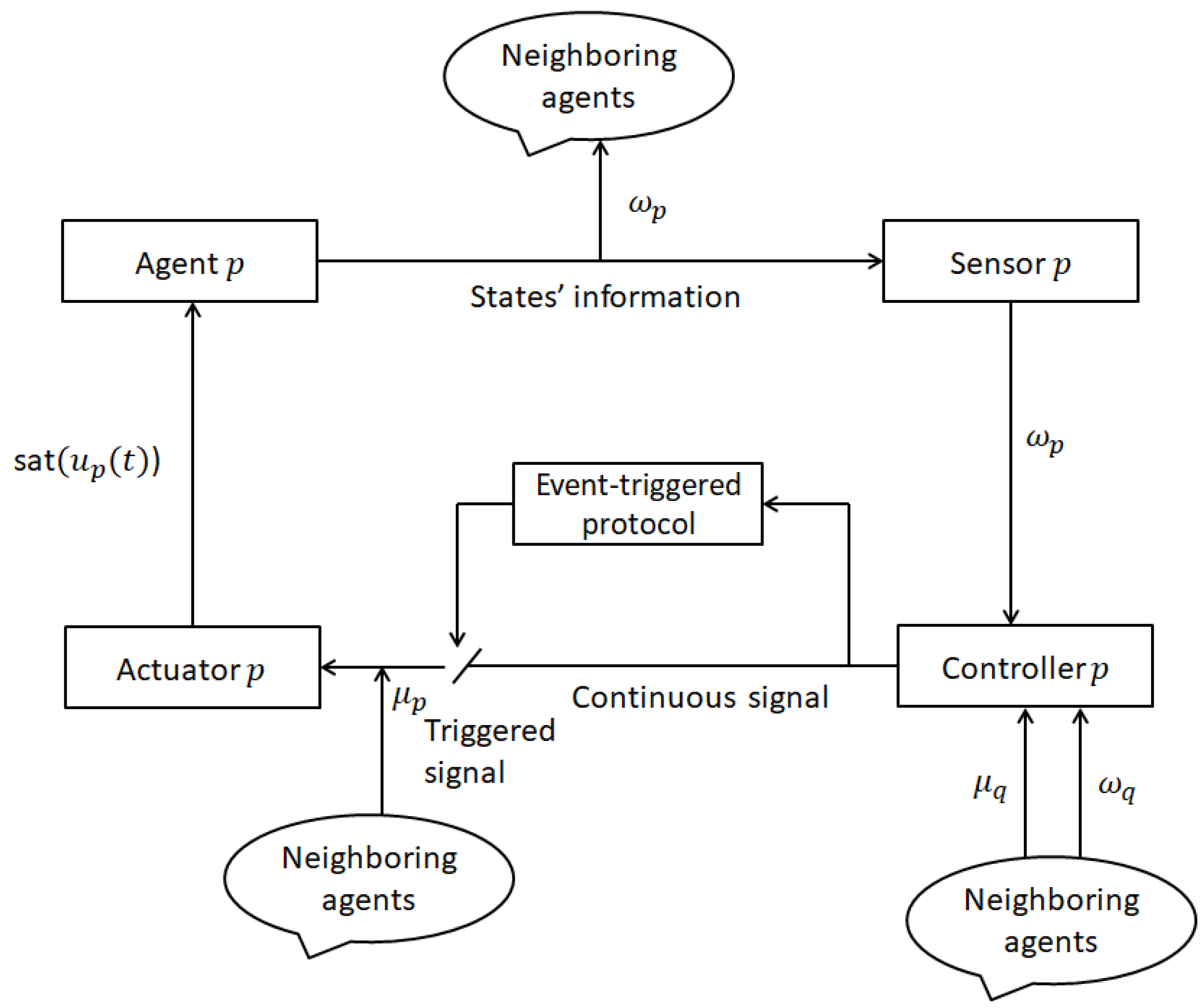
where denotes an adaptive parameter, and , and are positive constants that define DAETM (4). Moreover, Figure 1 displays the conceptual diagram of the proposed control method for the reader’s reference.
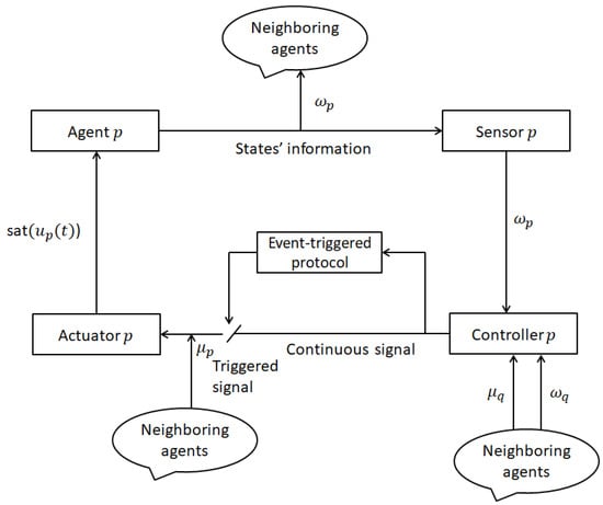
Figure 1.
Flow chart of the DAETM scheme with input saturation for agent p.
Define as the deviation between and the leader , and let be the measurement discrepancy for . Then, we have
where .
System (5) is rewritten in the following compact form:
where Then, the region of MAS (1) is defined as
Lemma 1
([13]). Let be a continuous vector function with a differentiable derivative. For , , and a symmetric positive matrix , the following relation holds:
Lemma 2
([26]). If matrices are given, and the vector x belongs to the set , defined as , then the saturation function lies within the convex hull denoted by of the set for all . Here, is a diagonal matrix with entries that are either 0 or 1, and , where is the identity matrix. The convex hull ensures that the result captures all possible linear combinations of the specified set, maintaining its bounded nature under the given conditions.
Lemma 3
([26]). Let the function be defined as , where represents the saturation function applied to the vector ω. For any diagonal positive definite matrix , if ω and ψ belong to the set
which is defined as the collection of all vector pairs ω and ψ whose maximum element-wise difference is bounded by , then the following inequality holds:
This inequality characterizes the behavior of the saturation deviation , the matrix T, and the vector ψ, ensuring stability within the specified set .
Lemma 4
([27]). Consider the matrices (a positive definite matrix), , and any constant l. The following inequality holds:
Assumption 1.
The graph G is considered connected, implying that a path exists between any two nodes within the graph, ensuring no node is isolated.
Assumption 2.
The vector function is said to satisfy the integral quadratic constraint if, for any , the following inequality is satisfied:
where is known as an incremental multiplier matrix. According to [28], Ξ can be expressed in the form
Assumption 3.
There is an unknown upper bound for the external disturbances such that .
4. Main Results
This section demonstrates that leader–follower FONMANSs (6) can achieve consensus using a sector-bounded approach and the convex hull method. Additionally, we show that Zeno’s behavior is avoided under certain reasonable assumptions.
4.1. Sector-Bound Condition Approach
In this subsection, we address the saturation term in the system dynamics by using the sector-bound condition. Actuator saturation is a type of “hard nonlinearity”, similar to dead zones, hysteresis, and backlash. To handle this, we introduce a sector nonlinearity model that ensures the solution to the consensus problem in leader–follower FONMASs (6). Based on previous studies [22,26], this approach effectively deals with nonlinearities, especially those caused by input limitations such as actuator saturation. Systems with saturation are difficult to analyze using the standard Lyapunov stability theory, so we must handle the saturation term first. The sector-bound condition ensures that the saturation function stays within a specific range, allowing the use of LMIs for stability analysis. The main idea is to transform the saturation term, , into a dead-band function , which enables the application of sector inequalities (see Lemma 3). Unlike low-gain feedback methods, the sector-bound condition and convex hull representation have a specific range of use, known as the consensus domain of attraction. Estimating this domain is a common challenge with these methods. A common approach is to use the Lyapunov function’s level set to estimate the consensus domain of attraction. Compared to the convex hull representation, the sector-bound condition has clear advantages in estimating this domain. As a result, the consensus problem in leader–follower FONMASs (6) can be relaxed using sector conditions that are effective globally.
- From (3), the control input can be expressed as
Theorem 1.
Consensus in leader–follower FONMANSs (6) can be attained with the DAETM (4), provided that positive constants , a positive diagonal matrix , and , , and ϝ satisfy the following conditions:
where , , ; denotes the qth component of matrix ϝ, , , then the consensus domain is approximated using the set .
Proof.
The Lyapunov function is selected as follows:
By employing Lemmas 1 and 2, we calculate the Caputo derivative by considering (6) and (8), and then derive that
By using Assumption 2, it follows that
According to Assumption 3, it is obtained that
Consequently, inequality (9) holds under the given conditions:
Accordingly, takes the form
where , and
To resolve the issue where condition (16) does not align with the conventional form of an LMI, an alternative method is employed. This method involves the decomposition of the matrix using an orthogonal matrix , such that , with containing the eigenvalues of . This allows for a reformulation of the system’s stability conditions in terms of the transformed state variables , leading to a simplified expression for stability analysis , which ensures the system’s stability by satisfying the necessary conditions in a more straightforward form:
where
As a result, (15) is equivalent to
Therefore, we can infer that if
The condition ensures the validity of the sector-bound condition; serves as a domain of consensus in this context, and its range is approximated by . It can also be concluded that if the following inequality is satisfied:
Given the characteristics of the Kronecker product, if we multiply Equation (20) by on both sides, we can derive the LMIs (10).
From (18), we have
Therefore, implying that the consensus of the leader–follower FONMANSs is achieved. This ensures that all agents converge to a common state, satisfying the consensus of the system condition. □
4.2. Convex Hull Representation Approach
In this subsection, we explore the application of a convex hull approach to handle a saturation term, denoted as . This is often used in control systems, optimization, or numerical methods, where saturation can be interpreted as a nonlinear operation that limits the output of a system or process.
The main idea is to represent the saturation function as a convex combination of multiple points or functions to manage its behavior. In Equation (8), the approach is outlined as follows:
The saturation term can be approximated or represented as a convex combination of several possible outcomes, expressed as
Thus, the convex combination approach allows for expressing the saturation term as a weighted sum of different terms that span the space of possible outcomes, providing flexibility in approximating or controlling the saturation behavior.
Remark 1.
Theorem 1 presents a practical way to calculate the gain matrix for the distributed consensus control strategy and the parameters of the DAETM (4), guaranteeing asymptotic stability and consensus in the leader–follower FONMANS systems (6). The gain matrix and ET threshold parameters γ, and θ are carefully derived from the feasible solutions of (9) and (10). These solutions are systematically constructed to achieve stability and minimize communication and computational overhead within the network. The derivation process depends on the agent-specific parameters and as well as the communication topology matrix which defines the interactions among leaders and followers. This approach provides a clear way to handle the relationships between agents and the network structure, ensuring smooth coordination and control. It is also designed to handle larger and more complex systems without adding too much computational load, making it suitable for practical applications.
Theorem 2.
Proof.
Consider the following Lyapunov function for analyzing the error dynamics of the system (6):
By Lemma 1, the Caputo derivative along the trajectory of (6) and (21) is obtained as follows:
By applying Lemma 3, the system’s behavior at each time t for each where r is indexed over the set can be analyzed. The computation of these elements is shaped by the structure and dynamics of the system, which may involve fractional differential equations. In particular, can be expressed as follows:
The specified expression is . Then, following the approach similar to that in Theorem 1, if the inequality below is satisfied, it leads to the conclusion that , as follows:
By applying Lemma 4, it follows that . Furthermore, it is established that the error region , which defines the acceptable bounds on the error, is a subset of the polyhedral region . This polyhedral region is defined as the set of error and measurement terms such that the norm of their weighted sum, influenced by the matrix , is a constrained constant, , i.e., . This inclusion enables the use of a geometric approximation, simplifying the analysis of the system’s behavior. The following inequality governs the system’s dynamics, describing the interaction between the error terms e, and the system matrices, ensuring that the overall system stability is maintained:
This inequality guarantees that the system’s trajectory remains within the prescribed error bounds, thus confirming that consensus is achieved under the given conditions. Based on the DAETM (4), if and only if , implying that, . fulfills the condition required for the introduction of the convex hull notation. Therefore, is the domain of the consensus in this context, and its domain is approximated by . Assuming , we proceed to analyze that
where . By applying the Schur complement, we can demonstrate that the following inequality leads to the result in (28) as follows:
By using the similar proof of Theorem 1, ensuring the system’s stability and consensus analysis,
where , , , and the domain of consensus is determined by the region . Consequently, consensus is achieved in the leader–follower FONMANSs. □
4.3. Zeno Behavior Analysis
This section demonstrates that Zeno behavior is avoided in leader–follower FONMANS systems (6) through the application of the DAETM strategy (4). By analyzing the conditions that prevent infinite switching within a finite time, the system’s smooth evolution is ensured, avoiding instability or non-physical behavior. Furthermore, the DAETM strategy establishes sufficient constraints on system parameters, effectively eliminating the risk of Zeno behavior and guaranteeing stable and predictable performance over time.
Theorem 3.
Given the conditions specified in Theorem 1, the leader–follower FONMANS systems (6) do not exhibit Zeno behavior, and the time interval between consecutive triggering instants for any agent remains strictly positive, i.e., .
Proof.
Based on the proof of Theorem 1, we establish that
the error between the agent p and its target trajectory converges to zero as time progresses. Furthermore, there exists a non-negative scalar such that
this establishes an upper bound for the -order derivative of the error function, ensuring that the error’s rate of change remains constrained. Based on Definition 2, we define a function that satisfies the relationship
where indexes the other agents in the system. This function represents the time evolution of the error between agents p and q. To simplify the analysis, we denote
which captures the rate of change of the error between the two agents. Finally, by applying the Laplace transform to the -order integration, we obtain an expression in the frequency domain, which is crucial for analyzing the stability and behavior of the system:
where and Hence, we obtain
This leads to
Therefore,
Consequently, the subsequent inequality is satisfied:
where
Then, we have
Thus, one obtains
Based on the ET function (4), it follows that
The interval between two triggering moments and can be made arbitrarily large if the evolution of is slow enough, which prevents the occurrence of Zeno behavior. By considering the monotonic properties of and the constraints placed by the error dynamics, we can establish a lower bound for the time between consecutive triggers. This bound ensures that the system will not exhibit arbitrarily frequent triggering events, thus maintaining stability and avoiding Zeno behavior:
Therefore, Zeno behavior is prevented for all agents, ensuring that the system’s triggering events remain sufficiently spaced apart, preventing any infinitely rapid sequences of updates.
Remark 2.
The expression (33) provides an estimate for the minimum time interval between two consecutive triggering instants, and which reflects the sensitivity of the ET mechanism. This interval is determined by several factors, including the system parameters and the Caputo-type fractional derivative order ζ, and the ET threshold parameters and Notably, for a given system described by Equation (4), increasing the threshold parameter results in a longer minimum interval This indicates that the system becomes less sensitive to small state changes, potentially reducing communication and computational demand while maintaining stability.
5. Illustrative Examples
This section validates the effectiveness and applicability of the proposed theoretical observations by verifying the numerical simulations of the leader–following SG system using the experimental range of parameter values. Additionally, a comparative example is provided with the fractional-order Chua’s system to highlight the advantages of the proposed control method and the effectiveness of the derived sufficient conditions. This demonstrates the efficiency of the proposed control scheme, its validation process, and the details provided in Algorithm 1. All simulations were conducted using the LMI Toolbox in MATLAB 2017a.
| Algorithm 1 Proposed DAETM-based FONMANS with input saturation |
| Step 1: System initialization Initialize system matrices network topology , scalars diagonal matrix and event-trigger thresholds and . Set the saturation threshold and controller gain . |
| Step 2: Control input calculation For each agent p, compute the control input : . Calculate the control input: . |
| Step 3: Apply saturation Apply the saturation function: Approximate the saturated control input as a convex combination: |
| Step 4: ET condition For each agent p, check the event-triggering condition: . If satisfied, update neighbor states and reset parameters. Otherwise, proceed without updates. |
| Step 5: Stability and consensus Check stability using LMIs. Achieve consensus by ensuring that , i.e., agents align with the leader’s state . |
| Step 6: Return results Return the final states of all agents, achieving consensus with the leader. |
| Step 7: Repeat Repeat the process for the next time interval . |
Example 1


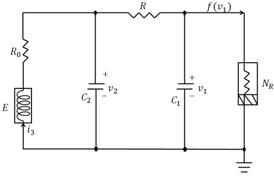
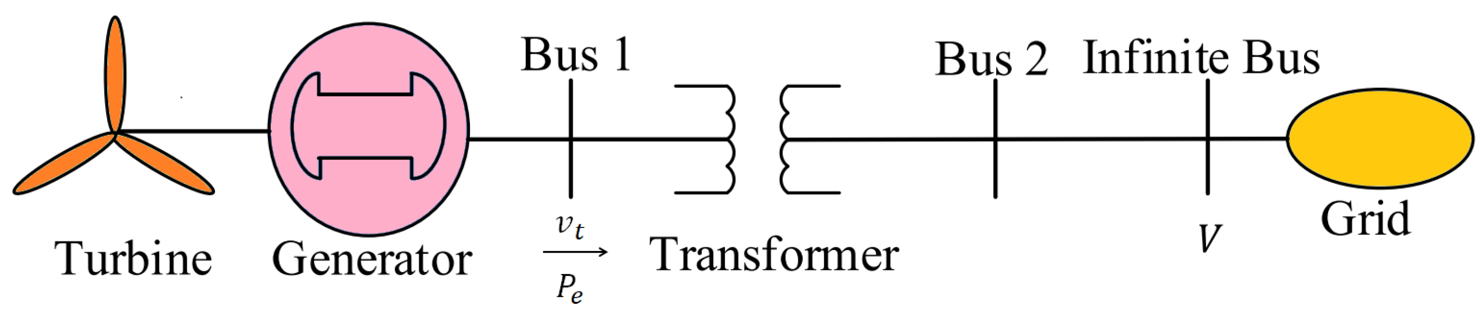
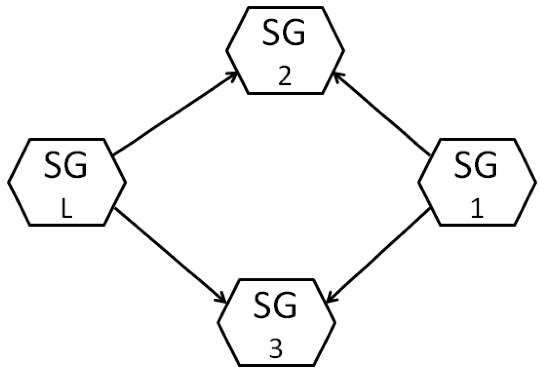
(Design Example). The modeling of practical power supply systems is very complex due to their nonlinear characteristics, strict operating criteria, and dynamic interactions between components. In this paper, an SG connected to an infinite bus via a transmission line is analyzed (Figure 2). In Figure 3, the agent with index L, and the agents indexed by , and 3 are referred to as the followers. Using the SG model described in [29] for measuring the rotor angle, the field voltage, rotor angle, and electrical power are among the essential measurable variables. Mathematical equations capture the nonlinear dynamics of this system and form the basis for the analysis of the system’s behavior. These equations help to determine the stability, control mechanisms, and performance of the system under different operating conditions.
Figure 2.
Structure of the SG connected to an infinite bus.
Figure 3.
Communication graph.
The following nonlinear equations define the model [29]:
where
Here, δ represents the rotor angle relative to the machine terminals and ω represents the rotor speed, along with other parameters used in the model, as stated in Table 1 (similar to [29]).
Table 1.
Symbols and descriptions of the SG model (34).
Under this assumption, magnetic saturation has no effect. Furthermore, the constants representing the increased reactance are , and . Below is a detailed overview of the system states and inputs:
The three state variables of the SG system are , , and Furthermore, the system disturbances are represented by , , and . Consider that the system inputs are and The dynamics of the leader and follower agents are described by the following fractional-order differential equations with a Caputo derivative:
Thus, the behavior of follower agents in a distributed SG system is defined by the following equation:
where are the state variables, is a defined nonlinear function, are the control inputs, and represents the external disturbances. Moreover , and are defined as follows:
Assume that For the numerical simulations, the parameter values in (35) are chosen as presented in Table 2, and the other parameter values are , , , , , , , and . Using the LMIs in (9) and (10), based on Theorem 1, we obtain the following:
Table 2.
Parameters of the SG model (34).
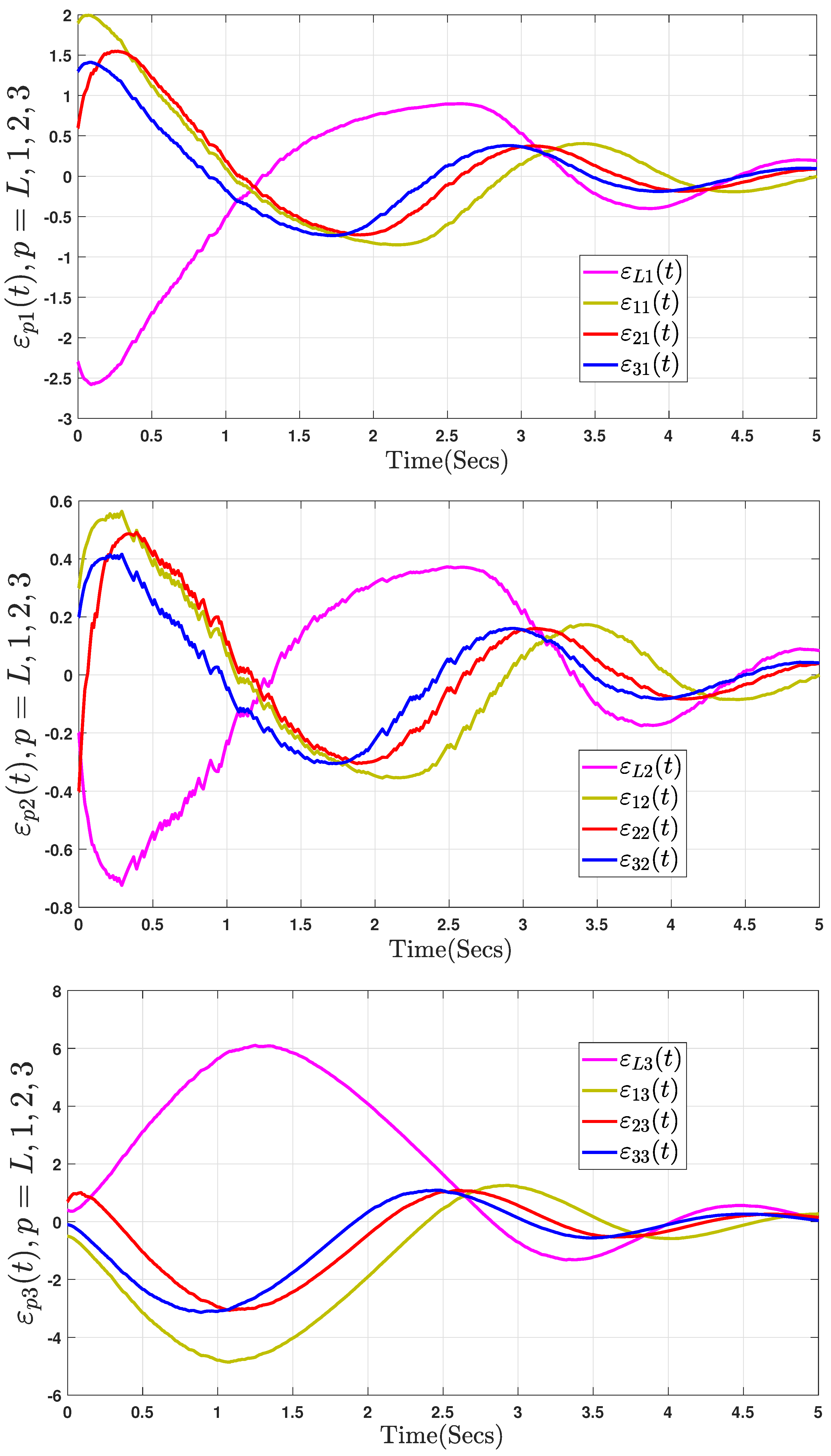
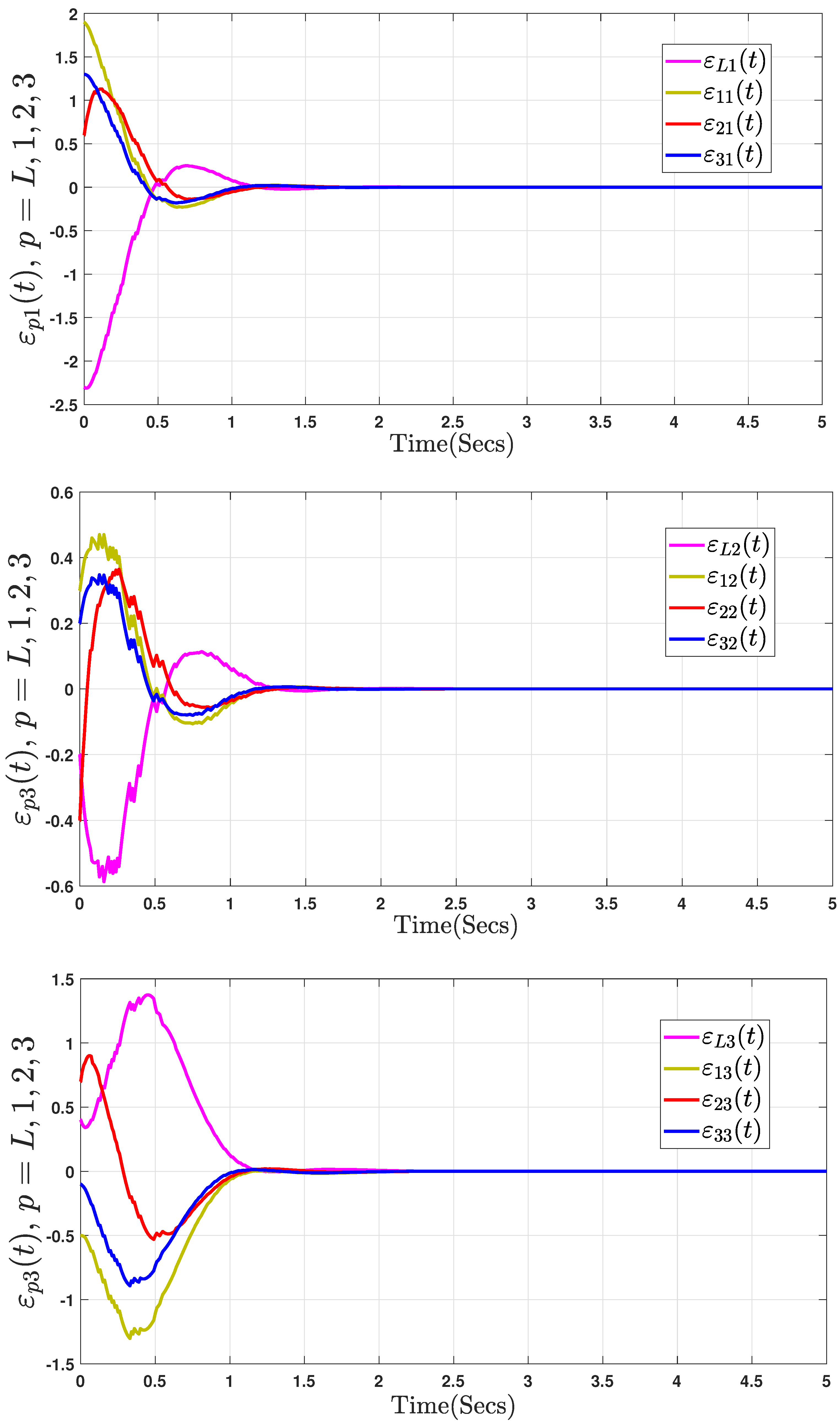
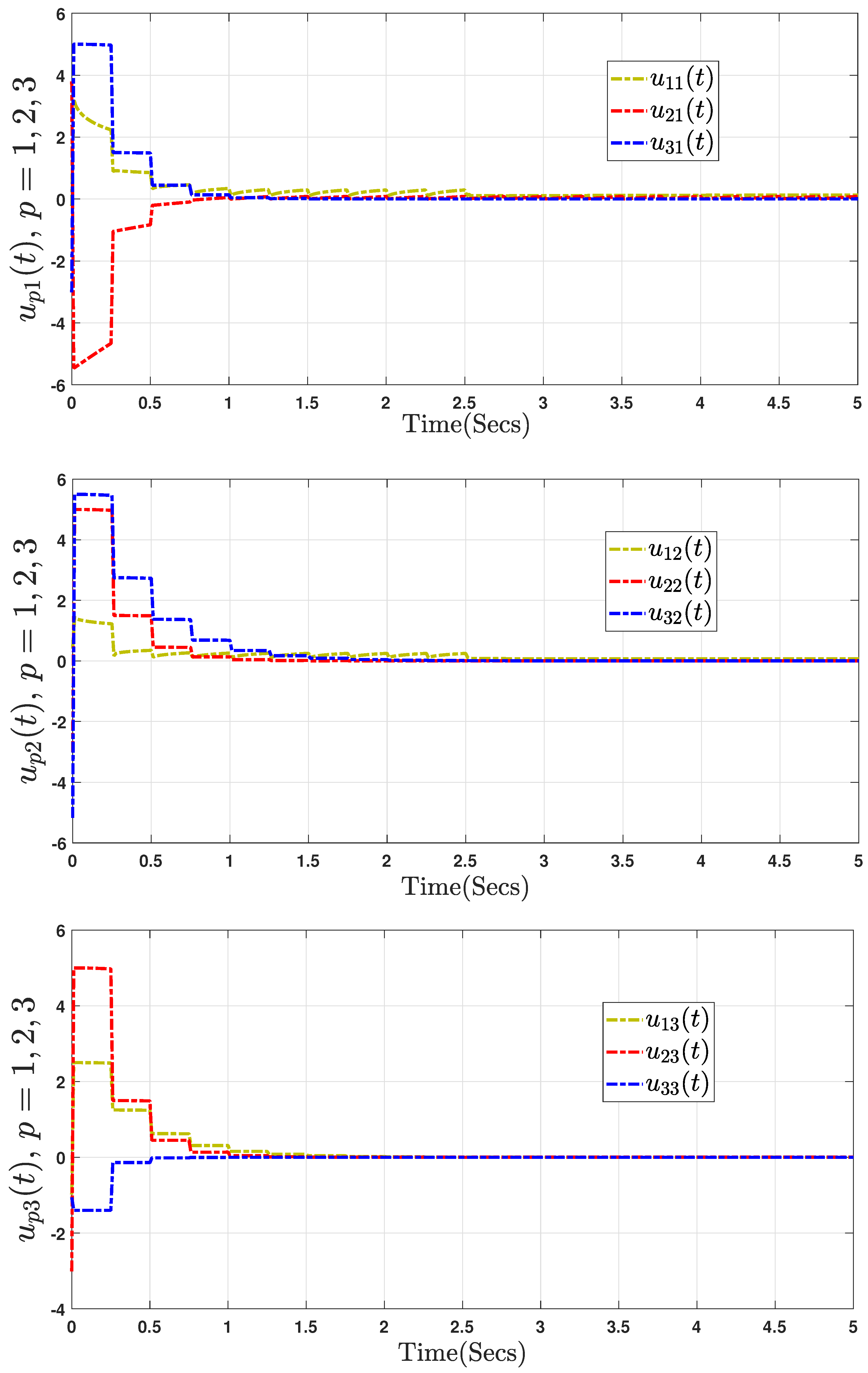
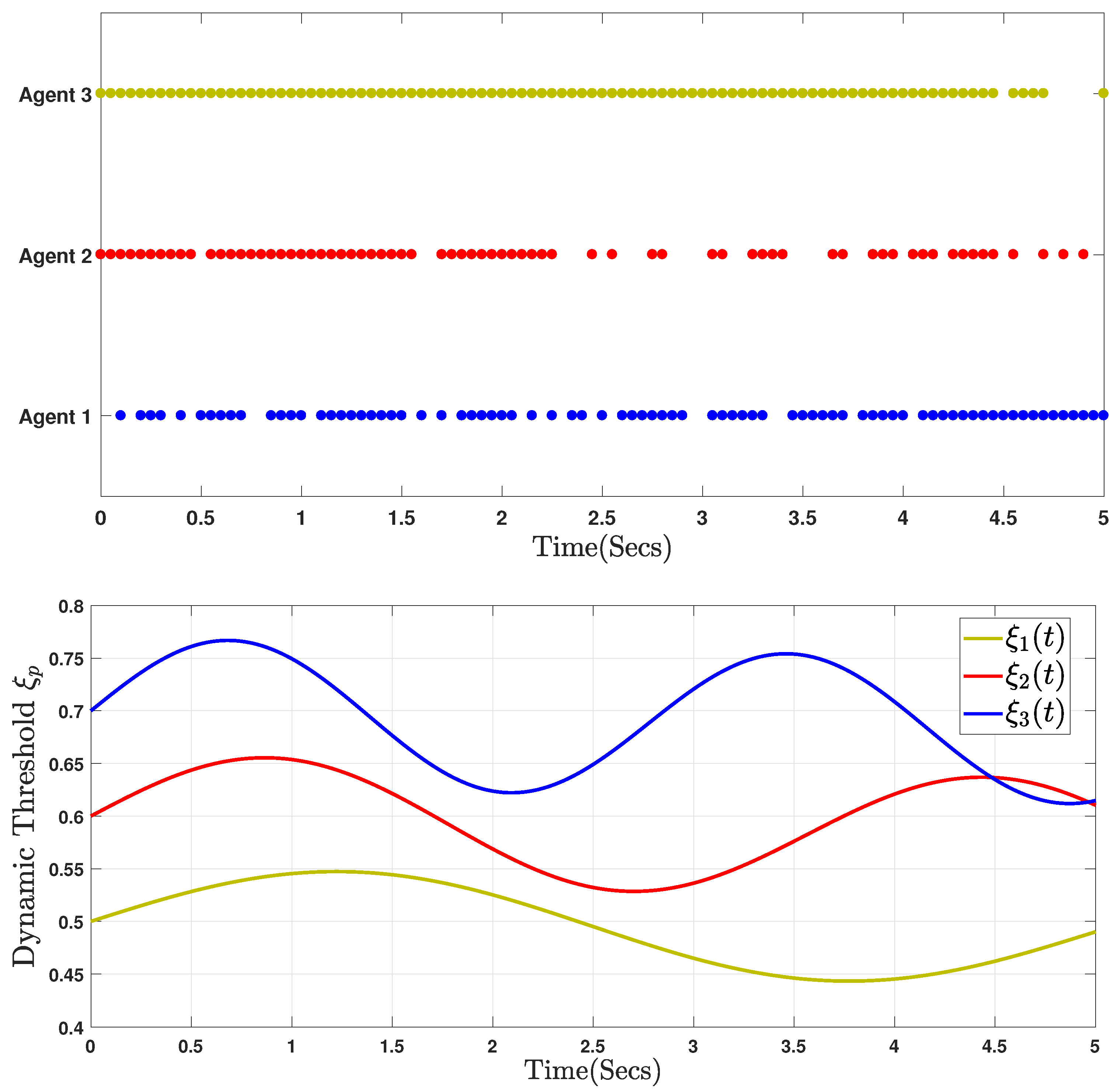
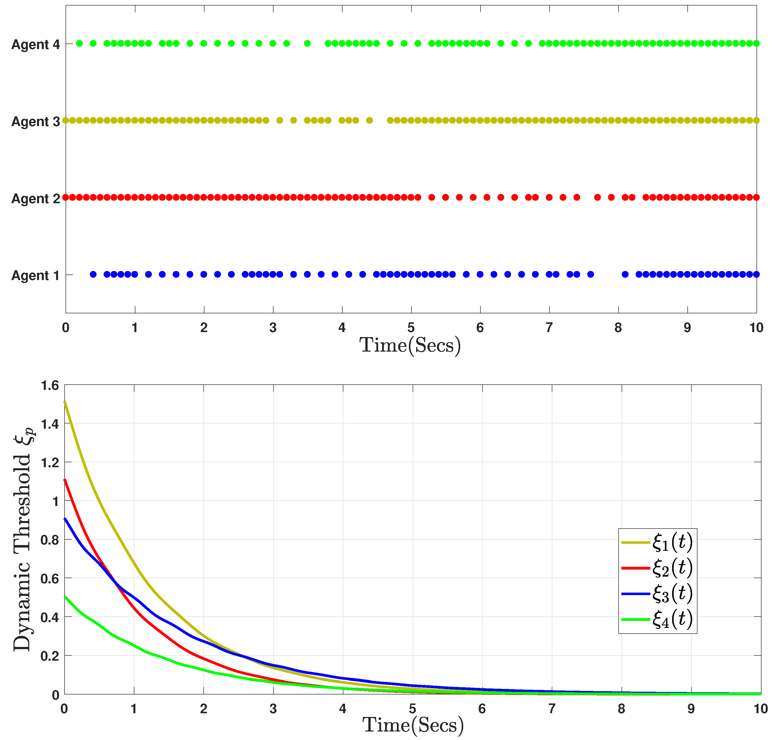
The simulation results are presented in Figure 4, Figure 5, Figure 6 and Figure 7, based on the initial conditions, , , , and , with the controller (3) and the DAETM (4) applied to each follower to control the trajectories of the state errors of the SG system. The analysis in Figure 4 clearly shows that the system is unstable, emphasizing the need to improve the controller’s robustness. The following discussion addresses key challenges such as actuator saturation, external disturbances, and limited communication, which are vital factors influencing the consensus problem of the fractional-order SG system defined by (37). Another key challenge was to ensure asymptotic consensus among agents in the fractional-order SG system (37) using the DAETM (4). Figure 5 demonstrates the tracking error system responses for the leader and three followers using the DAETM (4) based on the sector-bound condition approach. As illustrated in Figure 6, the proposed control inputs for the fractional-order SG system (37) are shown. Figure 7 shows the event-triggered update sequences for the three agents, corresponding to the DAETM scheme (4) and the dynamic ET protocol parameters for the three agents. These sequences illustrate how the control updates are triggered based on specific events rather than continuous monitoring, optimizing the efficiency of communication and computation. Additionally, the adaptive thresholds (see Figure 7) are observed to be bounded and dynamic, eventually converging from to Instead of being a fixed constant, the threshold is controlled based on the state variance, allowing the rate of data release to meet the dynamic control performance requirements. This dynamic adjustment ensures that the system remains flexible and responsive to varying conditions, improving performance while reducing unnecessary computations and communication delays. The parameters are essential for determining the timing of updates, ensuring that the agents’ responses stay synchronized while minimizing computational load. This approach enhances system stability and performance by triggering updates only when significant changes occur.

Figure 4.
Tracking error trajectories (37) without control input.
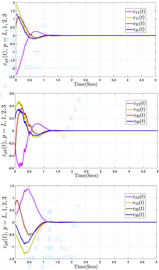
Figure 5.
Tracking error trajectories (37) with the DAETM scheme.
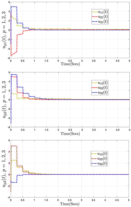
Figure 6.
Curves of the control input .

Figure 7.
Event-triggered instants of communication and the trajectories of dynamic variables .
The single-variable technique is used to investigate the effects of the fractional-order and the dynamic ET threshold parameter on the number of ET moments. The results, summarized in Table 3 and Table 4, reveal that the event-triggered method significantly reduces communication between agents. Table 3 shows that increasing the fractional-order substantially decreases the number of ET impulsive instances, while Table 4 demonstrates that increasing leads to more frequent ET impulsive instances. Additionally, we present the voltage and current evolutions for using the ET function (4), shown in Figure 6. As observed, a smaller value of , which corresponds to a higher error threshold (as indicated in Figure 6), results in slower convergence. This reflects a trade-off between communication frequency and convergence speed: higher values lead to faster convergence due to increased communication, while lower values reduce communication but result in slower convergence.
Table 3.
Number of events M for different values of with .
Table 4.
Number of instants M for various with .
This trade-off highlights the delicate balance between minimizing communication overhead and achieving the desired convergence speed. By adjusting it, it is possible to fine-tune the system’s performance, optimizing both the speed of convergence and the efficiency of communication, depending on the specific requirements of the application. The dynamic nature of these parameters offers flexibility in handling various system constraints and performance goals.
Example 2
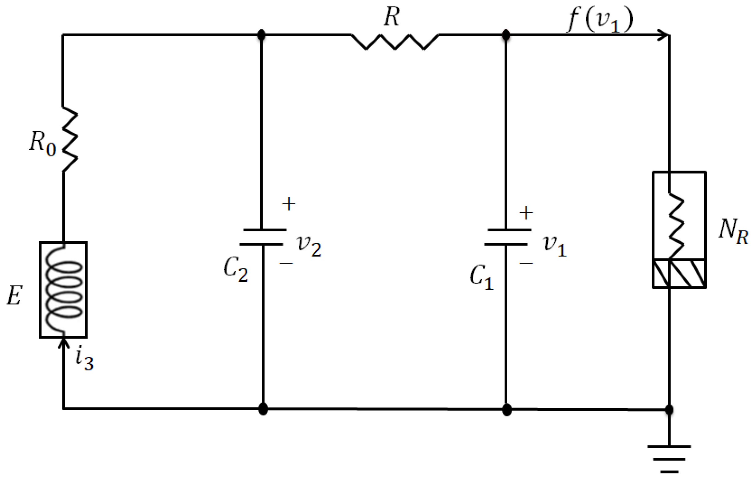
(Comparative Example). This subsection presents our results on the proposed control method for fractional-order Chua circuits [30]. The single-circuit model, shown in Figure 8, satisfies the following differential equations [30]:
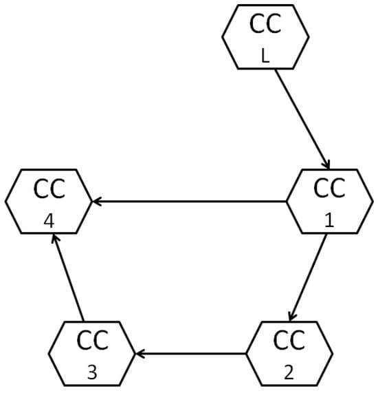
where the description of , , , , , L, , R, and are provided in [30]. Figure 9 shows the topological structure of the communication network, where a leader and four agents operate for a single Chua circuit.
Figure 8.
Structure of the Chua circuits.
Figure 9.
Communication graph.
Let , , and . The corresponding networked system can be expressed as
where In addition, , , and are defined as follows: We then select the following model parameters: and which follows a structure similar to that in [25]. It is established in [31] that satisfies Assumption 2. We assume that Chua’s circuit systems are applied with these model parameters to guarantee the stability of the FONMAS given in (40). The proposed values are , , , and Finally, using Theorem 1 and solving LMIs (9) and (10), it is observed that
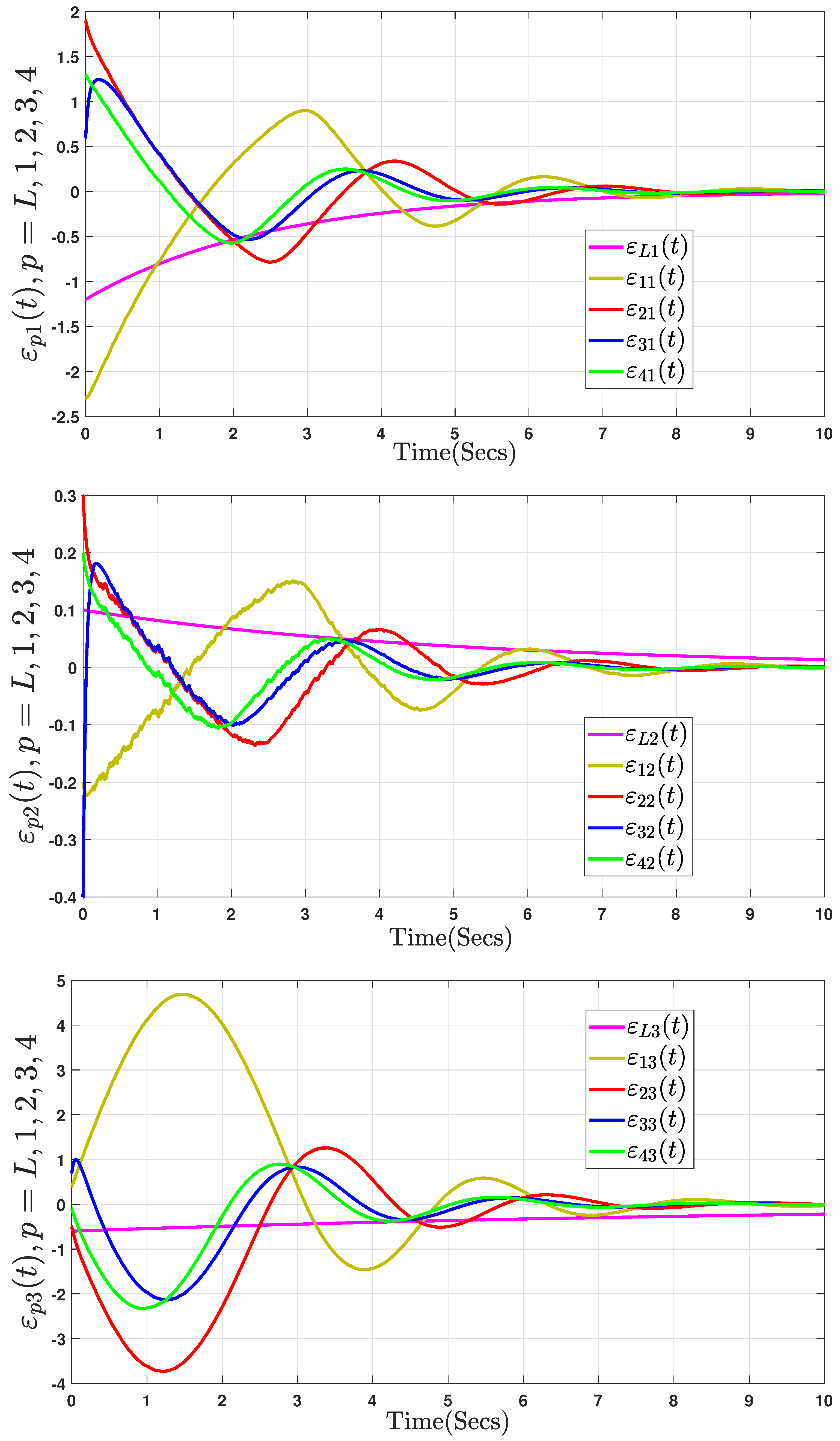
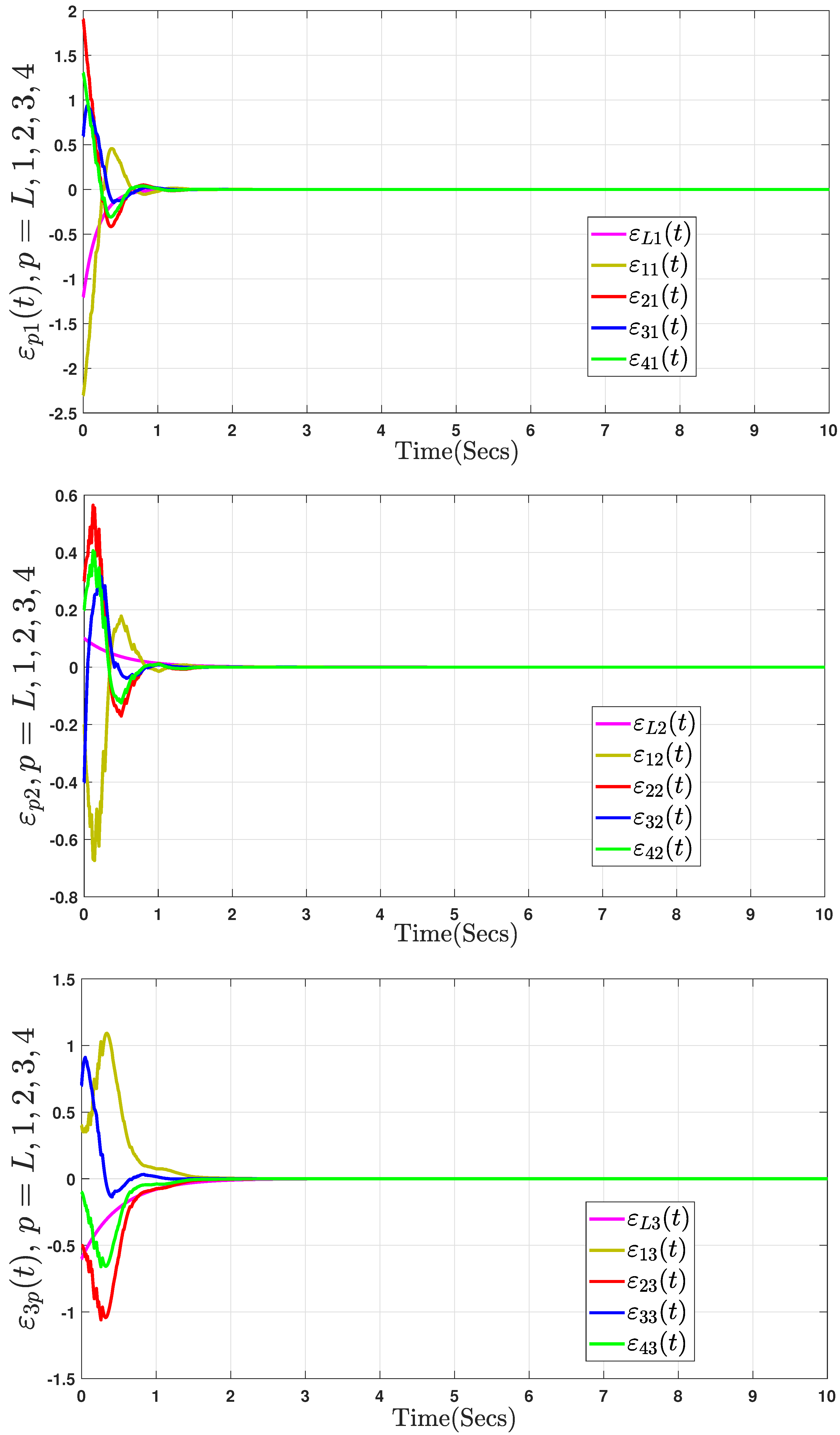
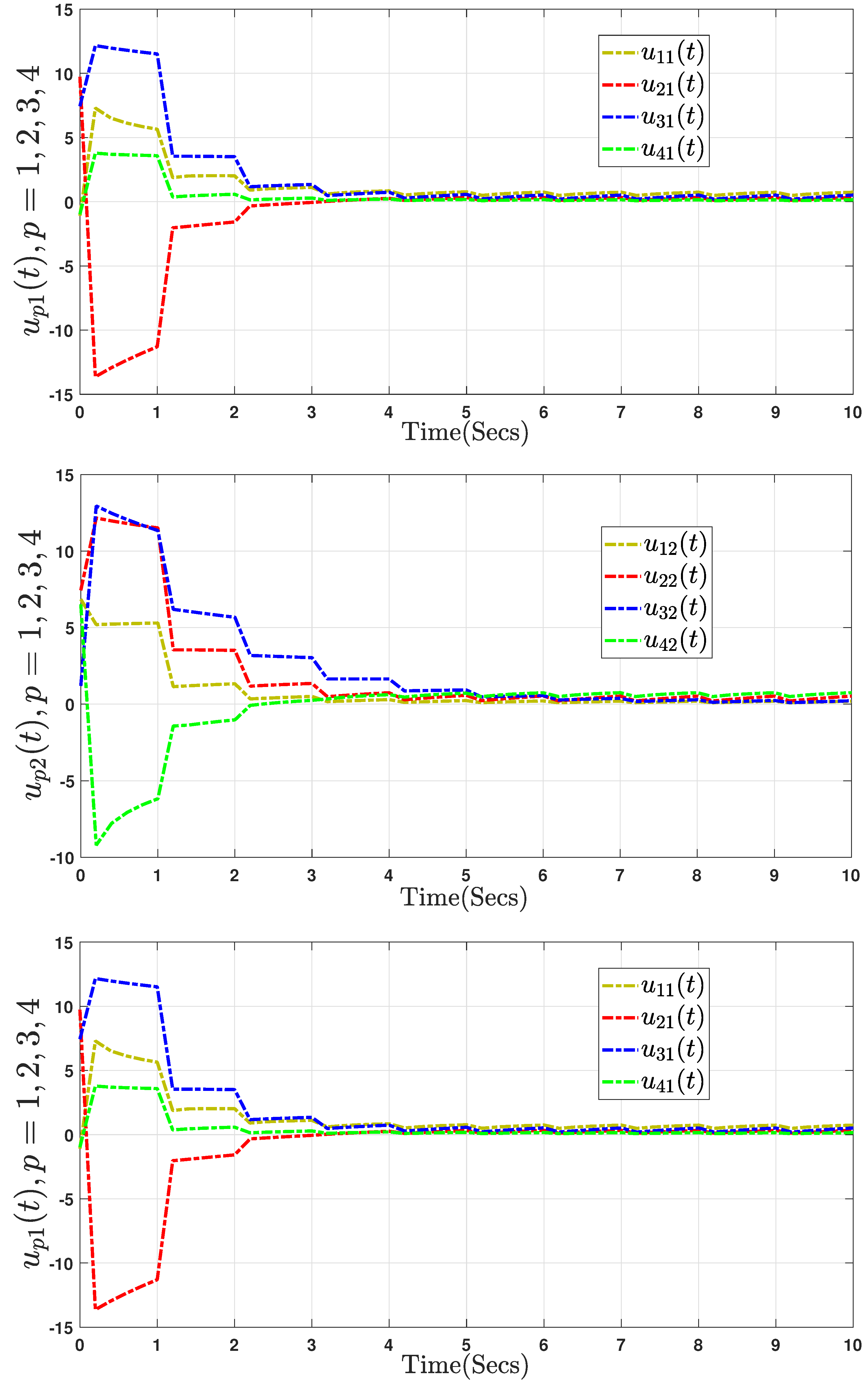
The initial state values of the system are and . Specifically, Figure 10 displays the state trajectories of fractional-order Chua’s system (40) without control input. The trajectories of the state errors are shown in Figure 11, Figure 12 and Figure 13. We propose the DAETM scheme (4) for each follower in the fractional-order Chua’s system (40), which consists of one leader and three followers. Figure 11 shows the responses of the tracking variables for the leader and the three followers using the DAETM scheme (4). Figure 12 shows the evolution of the control input for the three followers. Figure 13 illustrates the time points of the event triggering and the adaptive parameters Based on the analysis in Figure 11, Figure 12 and Figure 13, the dynamic variables used in the DAETM scheme demonstrate that the number of events triggered by the DAETM (4) with actuator saturation is significantly lower compared to the fixed-variable ET mechanism proposed in our study. This reduction in triggered events highlights the efficiency of the DAETM scheme in minimizing communication while maintaining synchronization among the agents. Moreover, by comparing the proposed DAETC mechanism in (4) with those in [16,18,20], which exhibit similar consensus performance, we conclude from Figure 13 and Table 5 that adopting the mechanism in (4) significantly reduces the communication burden. This reduction highlights the critical importance of selecting appropriate ET mechanism parameters to enhance the use of communication network bandwidth. In contrast to existing studies [16,18,20], our analysis demonstrates that the proposed strategy not only reduces data transmission but also improves overall system performance by increasing resource utilization and minimizing unnecessary communication. These results suggest that careful design of ET mechanisms can substantially enhance the efficiency of distributed systems.
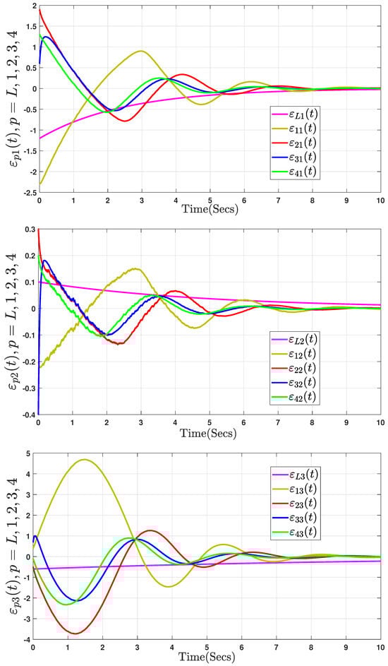
Figure 10.
Trajectory of tracking errors in (40) without control input.
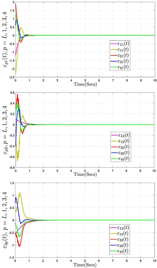
Figure 11.
Trajectory of tracking errors in (40) using the DAETM scheme.
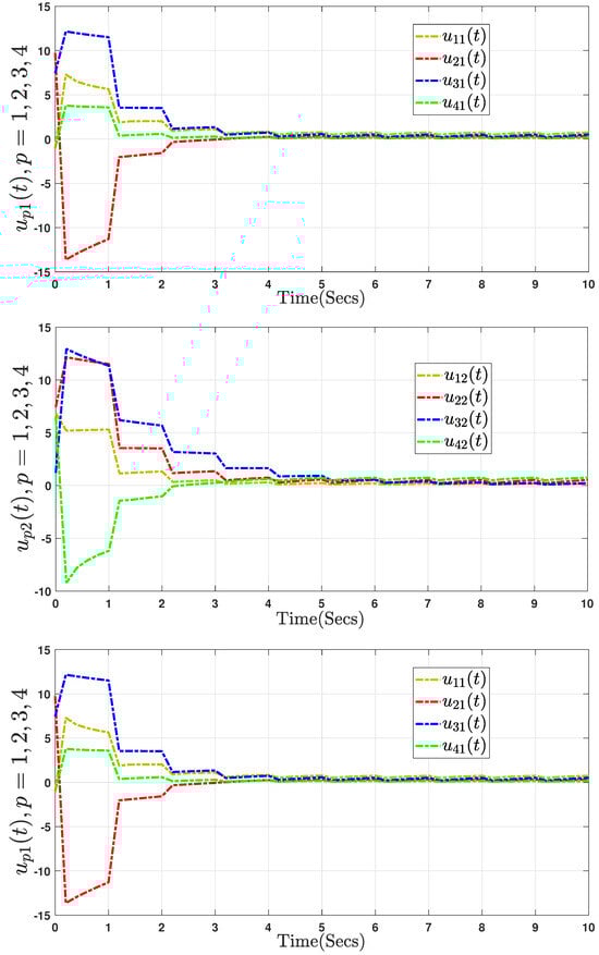
Figure 12.
Curves of the control input for Chua’s system in (40).
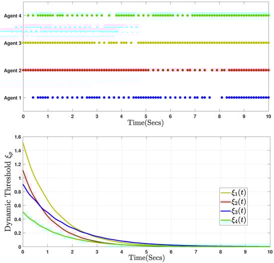
Figure 13.
Event-triggered instants of communication and the trajectories of dynamic variable .
Table 5.
The number of triggered events is compared with the methods of DAETC in [16,18,20].
6. Conclusions
In this study, we have addressed the event-triggered controller design for the consensus problem of leader–follower fractional-order nonlinear multi-agent networked systems, subject to actuator saturation and external disturbances. A novel dynamic adaptive event-triggered mechanism has been designed to handle actuator saturation, external disturbances, and limited communication while saving more communication resources than some existing methods. Two analysis approaches are presented to address the saturation term in the event-triggered controller design. By constructing an auxiliary fractional-order differential equation, a DAETM has been designed to significantly reduce the control transmission frequency while retaining the desired consensus performance. The sector-bounded and convex hull methods are applied, and by utilizing the properties of fractional-order calculus and Lyapunov functions, sufficient conditions in the form of LMIs are obtained to guarantee the asymptotic stabilization of the systems. Moreover, a positive lower bound has been established for the intervals of triggering instants to prevent Zeno behavior. Finally, numerical simulations of the fractional-order SG system demonstrate the effectiveness and superiority of the proposed approach. In the comparison studies of the fractional-order Chua circuit system, we have confirmed the feasibility of the proposed control method, showing that the DAETM method can effectively reduce the communication load. In our future work, based on the proposed adaptive event-triggered learning control algorithm [20,29], our objective is to investigate the challenges of learning control algorithms and actuator saturation in nonlinear leader–follower fractional-order multi-agent networked systems.
Author Contributions
Conceptualization, G.N. and M.B.; Methodology, G.N. and M.B.; Validation, V.G., G.N. and S.A.; Investigation, G.N., M.B. and S.A.; Writing—original draft, G.N.; Writing—review and editing, M.B., V.G. and S.A.; Visualization, G.N.; Supervision, S.A.; Funding acquisition, S.A. All authors have read and agreed to the published version of the manuscript.
Funding
This work was supported by the National Research Foundation of Korea (NRF) grant funded by the Korean government (MSIT) (No. NRF-2022R1A4A1023248 and No. RS-2023-00209794).
Data Availability Statement
Data sharing does not apply to this article as no datasets were generated or analyzed during the current study.
Conflicts of Interest
The authors have no relevant financial or non-financial interests to disclose. The authors declare that they have no conflicts of interest.
Abbreviations
The following key notations and abbreviations are used in this manuscript:
| Notations | Description |
| Non-negative integers | |
| Set of real numbers | |
| Set of complex numbers | |
| n-dimensional Euclidean space | |
| Set of all real matrices | |
| Set of positive integers | |
| Fractional-order derivative operator | |
| Fractional-order integral operator | |
| Gamma function | |
| ⊗ | Kronecker product |
| Diagonal matrix | |
| Matrix W is symmetric and positive-definite | |
| Transpose of a matrix W | |
| * | Non-diagonal symmetric entry |
| I | Identity matrix with compatible dimensions |
| Positive (semi) definite matrix | |
| Negative (semi) definite matrix | |
| The sign operator, that is, | |
| Convex hull | |
| , where is the eigenvalue of matrix | |
| Abbreviations | Meaning |
| MAS | Multi-agent system |
| SG | Synchronous generator |
| ET | Event-triggered |
| LMI | Linear matrix inequality |
| FOMAS | Fractional-order multi-agent system |
| DAETM | Dynamic adaptive event-triggered mechanism |
| FONMANS | Fractional-order nonlinear multi-agent networked system |
References
- Narayanan, G.; Ahn, S.; Wang, Y.; Jeong, J.H.; Joo, Y.H. Adaptive event-triggered stochastic estimator-based sampled-data fuzzy control for fractional-order permanent magnet synchronous generator-based wind energy systems. Expert Syst. Appl. 2025, 261, 125536. [Google Scholar] [CrossRef]
- Anbalagan, P.; Joo, Y.H. Stabilization analysis of fractional-order nonlinear permanent magnet synchronous motor model via interval type-2 fuzzy memory-based fault-tolerant control scheme. ISA Trans. 2023, 142, 310–324. [Google Scholar] [CrossRef] [PubMed]
- Narayanan, G.; Ali, M.S.; Zhu, Q.; Priya, B.; Thakur, G.K. Fuzzy observer-based consensus tracking control for fractional-order multi-agent systems under cyber-attacks and its application to electronic circuits. IEEE Trans. Netw. Sci. Eng. 2022, 10, 698–708. [Google Scholar] [CrossRef]
- Yan, X.; Li, K.; Yang, C.; Zhuang, J.; Cao, J. Consensus of fractional-order multi-agent systems via observer-based boundary control. IEEE Trans. Netw. Sci. Eng. 2024, 11, 3370–3382. [Google Scholar] [CrossRef]
- Khan, A.; Niazi, A.U.K.; Abbasi, W.; Awan, F.; Khan, M.M.A.; Imtiaz, F. Cyber secure consensus of fractional order multi-agent systems with distributed delays: Defense strategy against denial-of-service attacks. Ain Shams Eng. J. 2024, 15, 102609. [Google Scholar] [CrossRef]
- Gong, P.; Lan, W.; Han, Q.L. Robust adaptive fault-tolerant consensus control for uncertain nonlinear fractional-order multi-agent systems with directed topologies. Automatica 2020, 117, 109011. [Google Scholar] [CrossRef]
- Shahamatkhah, E.; Tabatabaei, M. Containment control of linear discrete-time fractional-order multi-agent systems with time-delays. Neurocomputing 2020, 385, 42–47. [Google Scholar] [CrossRef]
- Yang, Z.; Zheng, S.; Liu, F.; Xie, Y. Adaptive output feedback control for fractional-order multi-agent systems. ISA Trans. 2020, 96, 195–209. [Google Scholar] [CrossRef]
- Li, X.; Wen, C.; Liu, X.K. Sampled-data control based consensus of fractional-order multi-agent systems. IEEE Control Syst. Lett. 2020, 5, 133–138. [Google Scholar] [CrossRef]
- Chen, J.; Chen, B.; Zeng, Z. Synchronization and consensus in networks of linear fractional-order multi-agent systems via sampled-data control. IEEE Trans. Neural Netw. Learn. Syst. 2019, 31, 2955–2964. [Google Scholar] [CrossRef]
- Yu, Z.; Jiang, H.; Hu, C.; Yu, J. Necessary and sufficient conditions for consensus of fractional-order multiagent systems via sampled-data control. IEEE Trans. Cybern. 2017, 47, 1892–1901. [Google Scholar] [CrossRef] [PubMed]
- Chen, Y.; Wen, G.; Peng, Z.; Rahmani, A. Consensus of fractional-order multiagent system via sampled-data event-triggered control. J. Frankl. Inst. 2019, 356, 10241–10259. [Google Scholar] [CrossRef]
- Ye, Y.; Su, H.; Sun, Y. Event-triggered consensus tracking for fractional-order multi-agent systems with general linear models. Neurocomputing 2018, 315, 292–298. [Google Scholar] [CrossRef]
- Wang, H.; Chen, F.; Wang, Y. Co-design of distributed dynamic event-triggered scheme and extended dissipative consensus control for singular Markov jumping multi-agent systems under periodic Denial-of-Service jamming attacks. Expert Syst. Appl. 2024, 251, 124091. [Google Scholar] [CrossRef]
- Ge, X.; Han, Q.L.; Ding, L.; Wang, Y.L.; Zhang, X.M. Dynamic event-triggered distributed coordination control and its applications: A survey of trends and techniques. IEEE Trans. Syst. Man Cybern. Syst. 2020, 50, 3112–3125. [Google Scholar] [CrossRef]
- Han, Z.; Tang, W.K.; Jia, Q. Event-triggered synchronization for nonlinear multi-agent systems with sampled data. IEEE Trans. Circuits Syst. I Regul. Pap. 2020, 67, 3553–3561. [Google Scholar] [CrossRef]
- Deng, C.; Che, W.W.; Wu, Z.G. A dynamic periodic event-triggered approach to consensus of heterogeneous linear multiagent systems with time-varying communication delays. IEEE Trans. Cybern. 2020, 51, 1812–1821. [Google Scholar] [CrossRef]
- Xie, X.; Wei, T.; Li, X. Hybrid event-triggered approach for quasi-consensus of uncertain multi-agent systems with impulsive protocols. IEEE Trans. Circuits Syst. I Regul. Pap. 2021, 69, 872–883. [Google Scholar] [CrossRef]
- He, W.; Xu, B.; Han, Q.L.; Qian, F. Adaptive consensus control of linear multiagent systems with dynamic event-triggered strategies. IEEE Trans. Cybern. 2019, 50, 2996–3008. [Google Scholar] [CrossRef]
- Wang, J.; Zheng, Y.; Ding, J.; Zhang, H.; Sun, J. Memory-based event-triggered fault-tolerant consensus control of nonlinear multi-agent systems and its applications. IEEE Trans. Autom. Sci. Eng. 2024. [Google Scholar] [CrossRef]
- Pan, L.; Shao, H.; Li, Y.; Li, D.; Xi, Y. Event-triggered consensus of matrix-weighted networks subject to actuator saturation. IEEE Trans. Netw. Sci. Eng. 2022, 10, 463–476. [Google Scholar] [CrossRef]
- Fei, Y.; Shi, P.; Lim, C.C. Neural-based formation control of uncertain multi-agent systems with actuator saturation. Nonlinear Dyn. 2022, 108, 3693–3709. [Google Scholar] [CrossRef]
- Zhou, Y.; Li, C.; Jiang, G.P.; Liu, J. Robust prescribed-time consensus of multi-agent systems with actuator saturation and actuator faults. Asian J. Control 2022, 24, 743–754. [Google Scholar] [CrossRef]
- Podlubny, I. Fractional Differential Equations: An Introduction to Fractional Derivatives, Fractional Differential Equations, to Methods of Their Solution and Some of Their Applications; Elsevier: Amsterdam, The Netherlands, 1998. [Google Scholar]
- Narayanan, G.; Ali, M.S.; Alsulami, H.; Stamov, G.; Stamova, I.; Ahmad, B. Impulsive security control for fractional-order delayed multi-agent systems with uncertain parameters and switching topology under DoS attack. Inf. Sci. 2022, 618, 169–190. [Google Scholar] [CrossRef]
- Xu, J.; Huang, J. An overview of recent advances in the event-triggered consensus of multi-agent systems with actuator saturations. Mathematics 2022, 10, 3879. [Google Scholar] [CrossRef]
- Hu, S.; Yue, D. Event-triggered control design of linear networked systems with quantizations. ISA Trans. 2012, 51, 153–162. [Google Scholar] [CrossRef]
- Açıkmeşe, B.; Corless, M. Observers for systems with nonlinearities satisfying incremental quadratic constraints. Automatica 2011, 47, 1339–1348. [Google Scholar] [CrossRef]
- Sharifi, A.; Sharafian, A.; Ai, Q. Adaptive MLP neural network controller for consensus tracking of multi-agent systems with application to synchronous generators. Expert Syst. Appl. 2021, 184, 115460. [Google Scholar] [CrossRef]
- Ding, L.; Zheng, W.X. Network-based practical consensus of heterogeneous nonlinear multiagent systems. IEEE Trans. Cybern. 2016, 47, 1841–1851. [Google Scholar] [CrossRef]
- Jiang, G.P.; Tang, W.K.S.; Chen, G. A simple global synchronization criterion for coupled chaotic systems. Chaos Solitons Fractals 2003, 15, 925–935. [Google Scholar] [CrossRef]

Disclaimer/Publisher’s Note: The statements, opinions and data contained in all publications are solely those of the individual author(s) and contributor(s) and not of MDPI and/or the editor(s). MDPI and/or the editor(s) disclaim responsibility for any injury to people or property resulting from any ideas, methods, instructions or products referred to in the content. |
© 2025 by the authors. Licensee MDPI, Basel, Switzerland. This article is an open access article distributed under the terms and conditions of the Creative Commons Attribution (CC BY) license (https://creativecommons.org/licenses/by/4.0/).