Open-End Fund Investment with Dynamic Fund Flows and Passive Benchmarking: A Continuous-Time Stackelberg Game

Abstract

This paper develops a stylized continuous-time framework for open-end fund investment in which state-dependent fund flows, passive benchmarking, and strategic manager–investor interaction are modeled jointly. The contribution is not a new Stackelberg solution concept; rather, it is the economic mechanism created by combining a scale-dependent value-added objective with endogenous subscription and redemption jumps. Fund flows are represented by marked compound Poisson processes, and the manager acts as leader while a representative investor chooses participation as a follower. Under bounded controls, bounded Lipschitz jump intensities, admissible jump-size distributions, and strict-concavity conditions, we establish positivity and moment bounds for the state process, provide sufficient conditions for the existence and uniqueness of a Markov feedback Stackelberg equilibrium, and state a jump-diffusion verification theorem. A transparent local feedback approximation and Monte Carlo robustness exercise illustrate how redemption pressure, subscription intensity, jump-size dispersion, benchmark volatility, and risk aversion affect active exposure and terminal fund wealth. The results show that stronger redemption pressure and benchmark-relative risk reduce active positions, whereas subscription incentives increase risk-taking only when expected value added compensates for flow-induced dilution. Within its stated assumptions, the model provides a tractable theoretical benchmark rather than an empirically validated structural model.

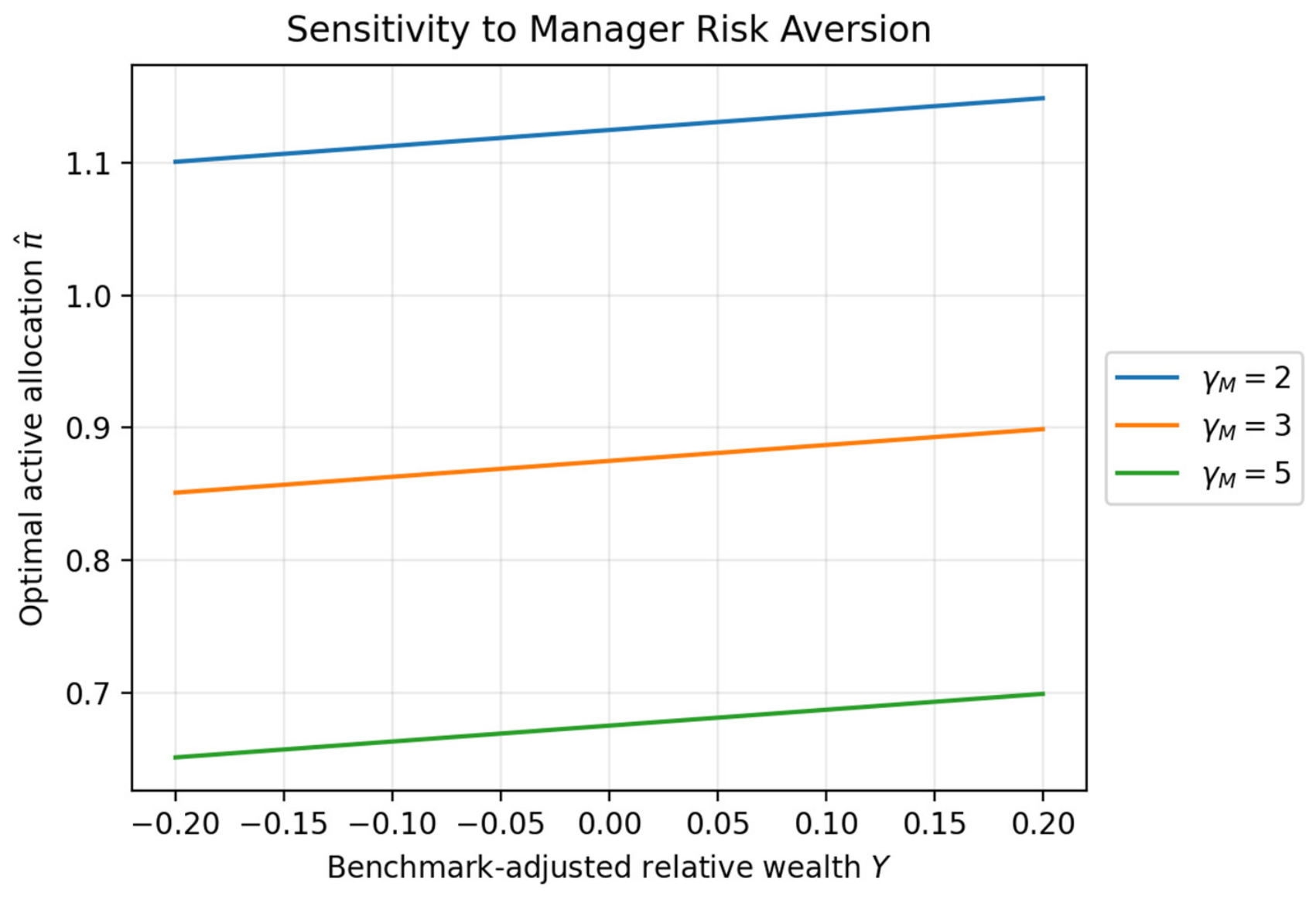
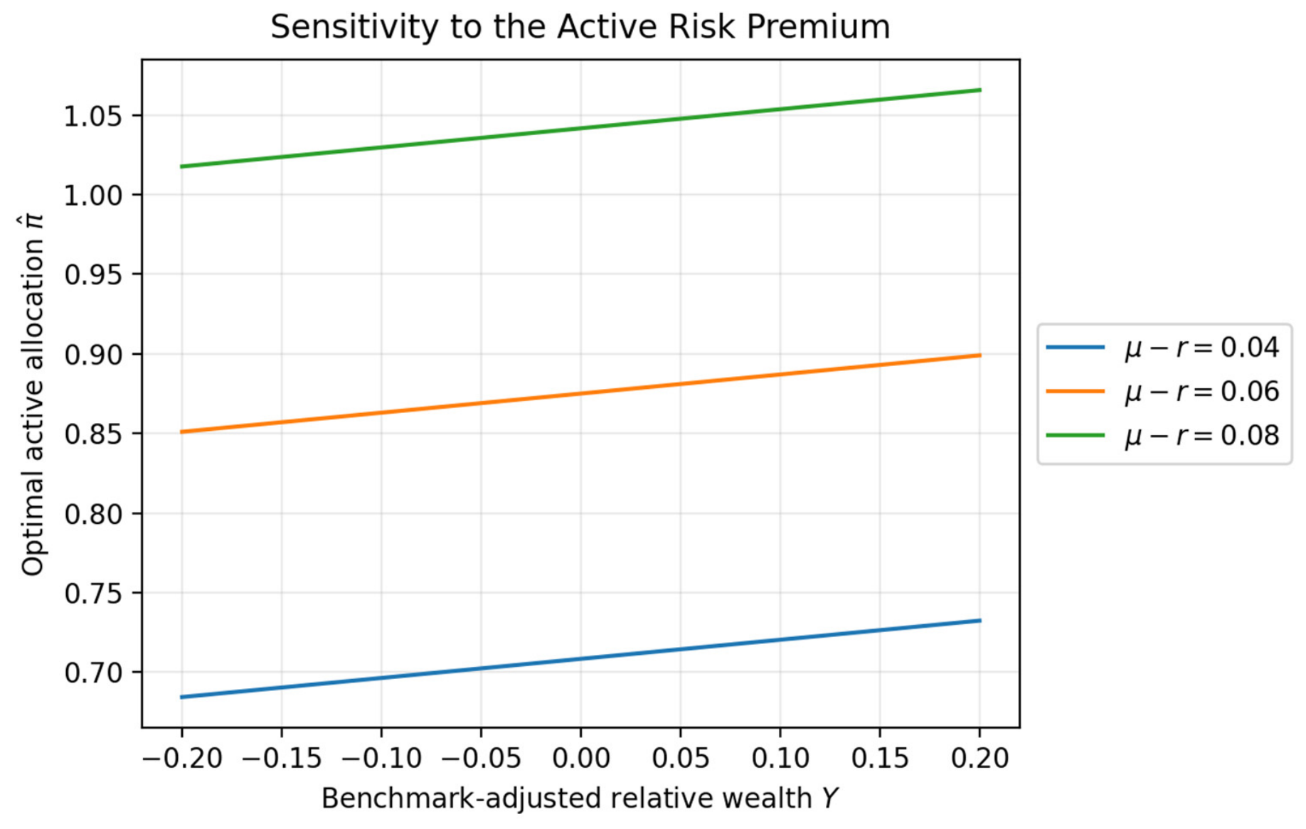
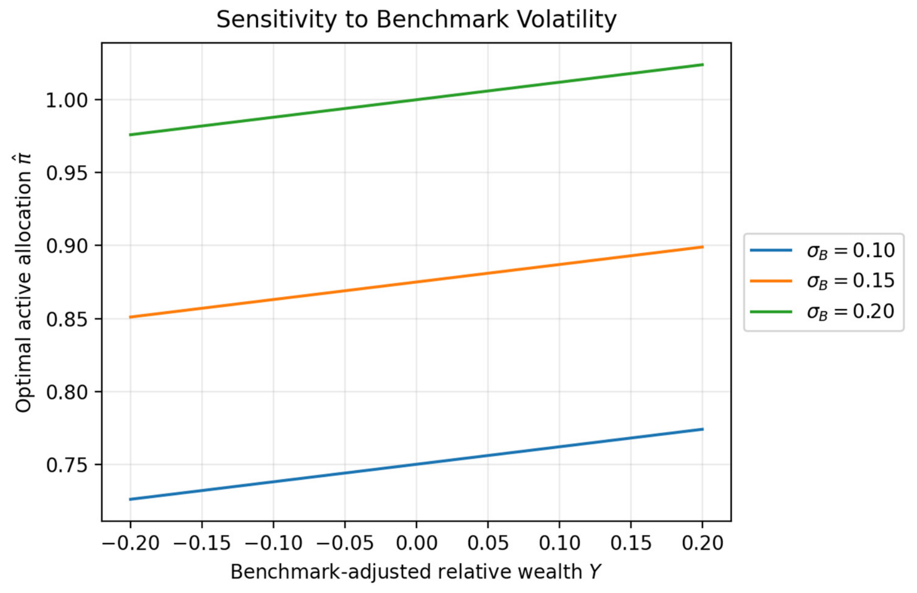
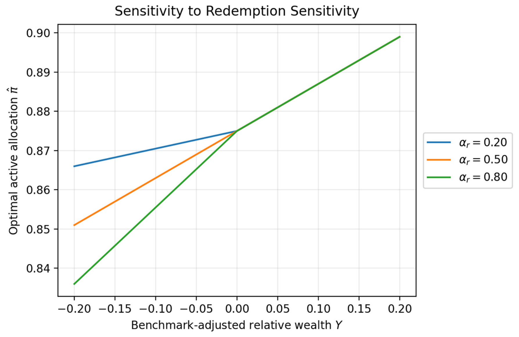
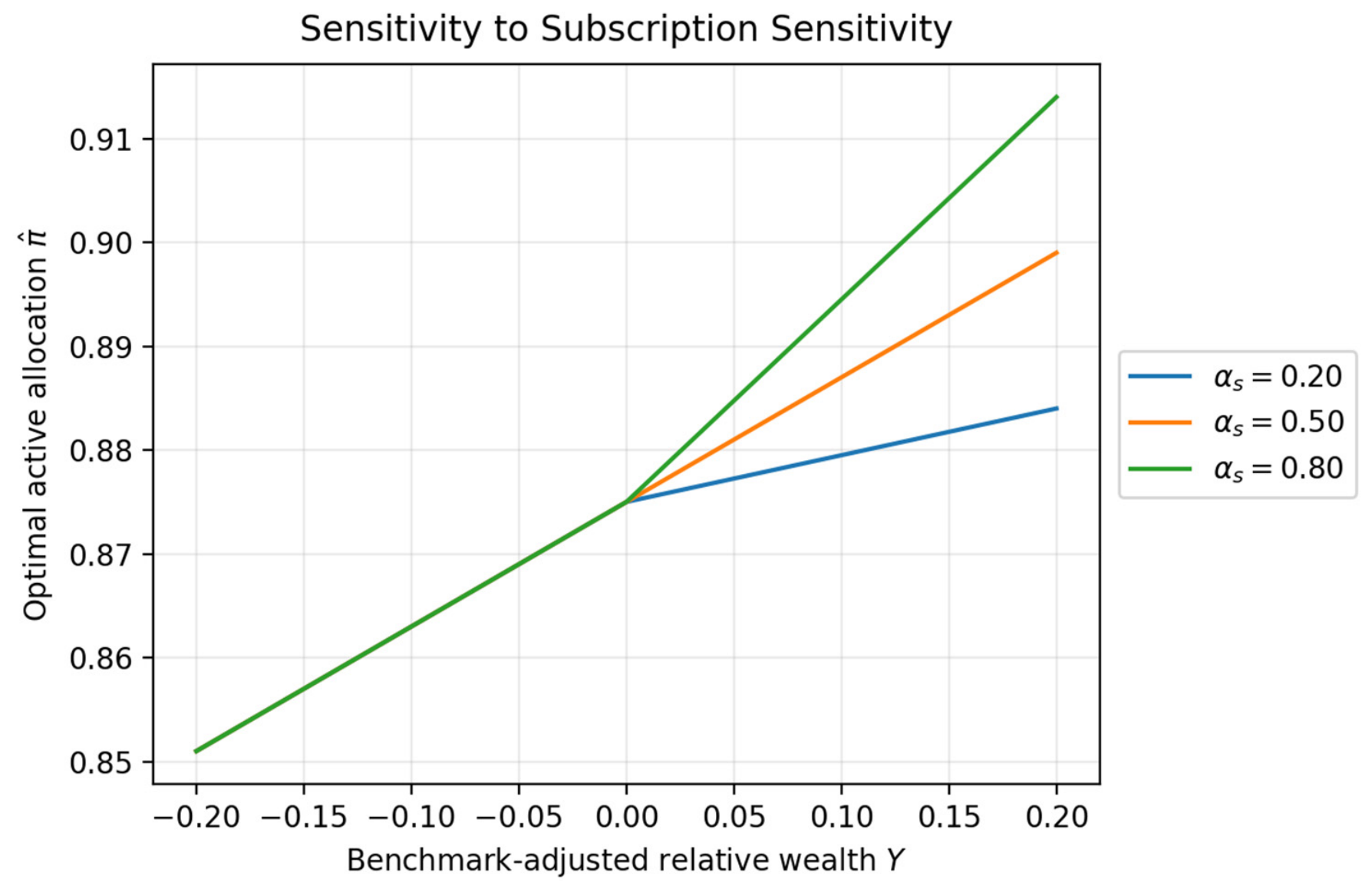
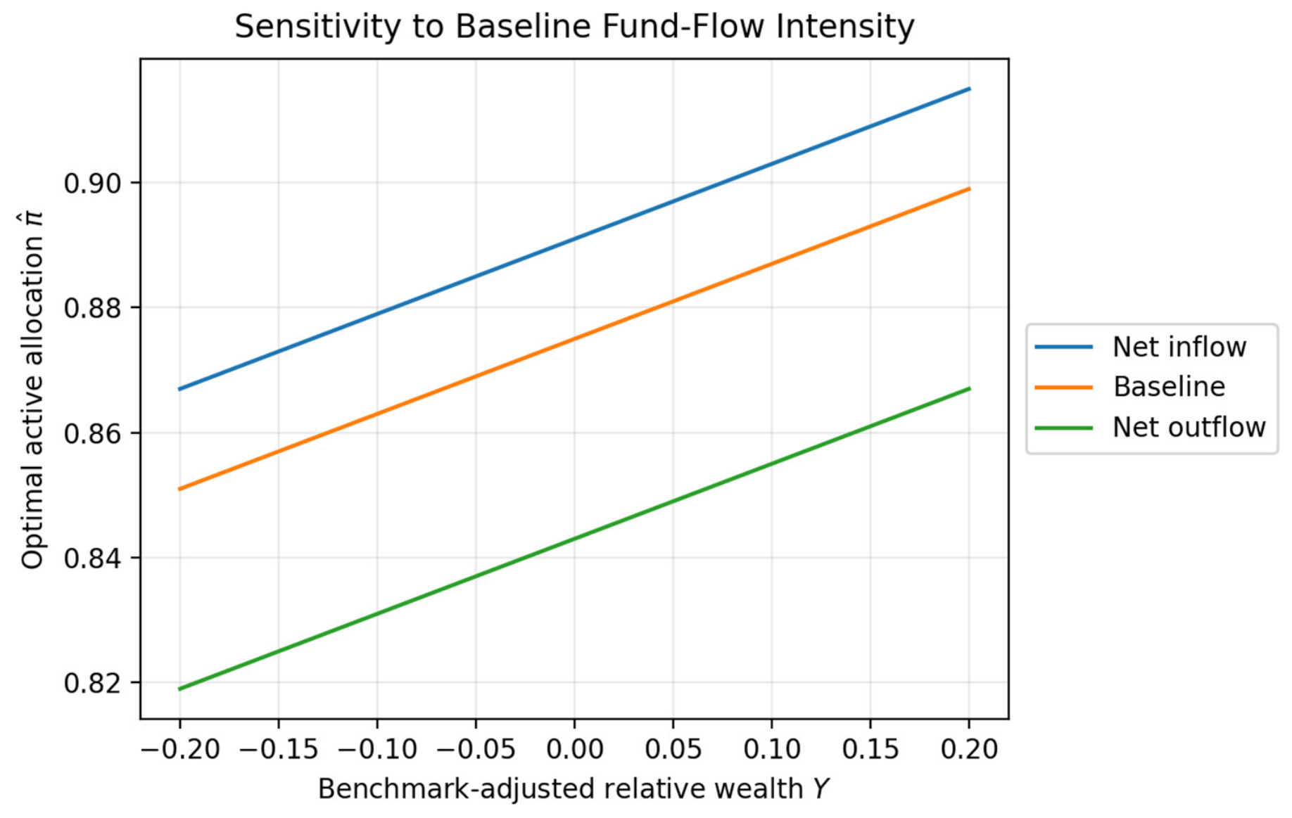
1. Introduction

Open-end funds combine delegated portfolio choice with a balance sheet that changes whenever investors subscribe or redeem. Consequently, a manager’s active allocation affects not only investment returns but also benchmark-relative performance, investor participation, and the future scale on which value added is produced.

The empirical fund-flow literature documents performance-sensitive allocations, participation frictions, and stronger outflow responses when liquidity is limited [1,2,3,4,5,6,7,8,9,10,11]. These findings motivate treating fund flows as economically consequential state transitions rather than as bookkeeping adjustments.

Continuous-time delegated-management studies emphasize benchmark incentives, contracts, and strategic portfolio choice. Basak et al. [12] analyze risk shifting under relative-performance incentives; Han et al. [13] formulate an active–passive mutual-fund Stackelberg game; Ou-Yang [14] and Cuoco and Kaniel [15] study continuous-time delegation and benchmark-linked contracts; Davis and Lleo [16] examine benchmarked risk-sensitive asset management. Rigorous jump-control and stochastic-game foundations are developed in Øksendal and Sulem [17], Pham [18], and Browne [19].

The remaining gap is narrower than a claim of a fundamentally new mathematical methodology. Existing models generally do not combine, in one finite-dimensional Markov framework, an investable passive benchmark, scale-dependent accumulated value added, discontinuous subscriptions and redemptions, and a follower response that changes the arrival intensities of those flows.

The research question is therefore: how does an active open-end fund manager adjust benchmark-relative risk when investor participation endogenously changes subscription and redemption intensities? We model the manager as the leader and the representative investor as the follower and solve the game in Markov feedback form.

The paper makes three specific contributions. First, it links the dollar value of benchmark-adjusted performance to stochastic assets under management. Second, it introduces state-dependent marked jumps into the manager–investor feedback channel. Third, it derives the coupled HJB integro-differential system and gives sufficient conditions for state well-posedness, equilibrium existence and uniqueness, and verification.

Relative to Basak et al. [12], the present model does not focus on compensation-induced risk shifting; it focuses on how subscriptions and redemptions change fund scale and continuation value. Relative to Han et al. [13], the follower is an investor whose participation controls open-end fund-flow intensities, rather than a competing passive-fund manager. Thus, the novelty is the interaction of these ingredients, not a new game-theoretic equilibrium concept.

The model is intentionally stylized. Constant investment opportunities and compound Poisson flows provide a transparent baseline, but they do not capture stochastic volatility, persistent flows, common liquidity shocks, delayed disclosure, or heterogeneous investors. We therefore interpret the results as qualitative comparative statics and describe empirical calibration and richer Cox/Hawkes-flow extensions in Section 4.

For managers, the framework separates direct active demand, benchmark-hedging demand, and flow-management demand. For investors and regulators, it highlights how redemption sensitivity can amplify the consequences of benchmark underperformance. A structured comparison with the closest continuous-time models is provided in

Table 1. Positioning relative to selected continuous-time fund-management models.

Study	Strategic Setting	Fund-Flow Treatment	Benchmark Treatment	Distinctive Mechanism
Basak et al. [12]	Manager optimization under incentives	Flow incentives are indirect	Relative-performance benchmark	Risk shifting and incentive effects
Han et al. [13]	Active–passive fund Stackelberg game	No open-end marked-flow state	Active versus passive funds	Strategic fund competition
Davis and Lleo [16]	Single-agent benchmarked control	No endogenous open-end flows	Risk-sensitive benchmark	Filtering and benchmark outperformance
Present study	Manager–investor feedback Stackelberg game	State-dependent subscription/redemption jumps	Investable passive benchmark	Scale-dependent value added plus endogenous flow intensities

.

The remainder of the paper is organized as follows. Section 2 specifies the market, fund flows, objectives, game, and admissible controls. Section 3 presents the HJB system, well-posedness and equilibrium results, and concise comparative statics. Section 4 explains the numerical method, parameter mapping, and robustness exercise. Section 5 concludes and states the limitations. A consolidated notation guide is provided in

Table 2. Core notation and economic interpretation.

Symbol	Definition	Domain/Assumption	Economic Role
X(t)	Open-end fund assets under management	X(t) > 0	Scales dollar value added and changes with returns and flows
B(t)	Passive benchmark net asset value	B(t) > 0	Investable outside option and performance reference
Y(t)	log[X(t)/B(t)]	Real-valued	Benchmark-adjusted relative-wealth state
π(t)	Manager’s risky-asset allocation	[π_min, π_max]	Leader control
u(t)	Investor participation intensity	[0, ū]	Follower control
r, μ, σ	Risk-free rate, active return, volatility	Bounded	Investment opportunity set
μ_B, σ_B, ρ	Benchmark return, volatility, correlation	σ_B > 0; |ρ| ≤ 1	Benchmark-relative drift and variance
λ_s, λ_r	Subscription/redemption intensities	Non-negative, bounded	Arrival rates of marked flow jumps
ξ_s, ξ_r	Subscription/redemption jump sizes	ξ_s ≥ 0; 0 ≤ ξ_r < 1	Preserve positivity and determine flow dispersion
γ_M, γ_I	Manager/investor risk aversion	Positive	Penalize benchmark-relative variance
δ_M, δ_I	Manager/investor discount rates	Non-negative	Weight continuation values
θ, c_I	Performance sensitivity, participation cost	θ ≥ 0; c_I > 0	Determine follower response
m(π)	Expected benchmark-adjusted return	Defined in Section 2.1	Direct active-performance component
v2(π)	Benchmark-relative variance	Defined in Section 2.1	Tracking-risk component
b_Y(π)	Continuous drift of Y(t)	Defined in Section 2.1	Relative-wealth state drift

.

2. Problem Formulation

2.1. Financial Market and Passive Benchmark

We consider a continuous-time financial market over a finite time horizon $[0,T]$. The uncertainty is described by a complete filtered probability space ${\displaystyle (}\mathsf{\Omega },\mathcal{F},\{{\mathcal{F}}_t{\}}_{0\le t\le T},\mathbb{P}{\displaystyle )},$ where $\{{\mathcal{F}}_t{\}}_{0\le t\le T}$ satisfies the usual conditions. Let $W^S{\displaystyle (}t{\displaystyle )}$ and $W^B{\displaystyle (}t{\displaystyle )}$ be two standard Brownian motions representing, respectively, the risk source of the actively managed risky asset and the risk source of the passive benchmark. Their instantaneous correlation is given by

$$d⟨W^S,W^B{⟩}_t=\rho \hspace{0.17em}dt, -1<\rho <1.$$

The parameter $\rho$ captures the degree of co-movement between the active investment opportunity and the benchmark index. A higher value of $\rho$ implies that the active risky asset is more strongly exposed to the same systematic risk as the passive benchmark, whereas a lower value of $\rho$ indicates greater potential for active diversification.

The market contains a risk-free asset $S_0{\displaystyle (}t{\displaystyle )},$ whose price process evolves according to

$$d{S}_0\left(t\right)=r{S}_0\left(t\right)dt, S_0\left(0\right)=1,$$

where $r>0$ denotes the constant risk-free interest rate. The actively managed risky asset $S{\displaystyle (}t{\displaystyle )}$ follows a geometric Brownian motion, namely

$${\displaystyle \frac{dS{\displaystyle (}t{\displaystyle )}}{S{\displaystyle (}t{\displaystyle )}}}=\mu \hspace{0.17em}dt+\sigma \hspace{0.17em}d{W}^S{\displaystyle (}t{\displaystyle )}, S{\displaystyle (}0{\displaystyle )}>0,$$

where $\mu$ is the expected rate of return and $\sigma >0$ is the volatility. This diffusion specification is standard in continuous-time portfolio choice and asset-pricing models, following the classical framework of Merton’s intertemporal portfolio selection model and the Black–Scholes diffusion setting. We assume that $\mu >r,$ so that the actively managed risky asset carries a positive risk premium:

$$\lambda ={\displaystyle \frac{\mu -r}{\sigma }}.$$

In addition to the active investment opportunity, investors can allocate their wealth to a passive benchmark fund, such as a broad market index fund or an exchange-traded fund [20]. The benchmark is not controlled by the active fund manager; rather, it represents the outside passive investment opportunity available to investors. Let $B{\displaystyle (}t{\displaystyle )}$ denote the net asset value of the passive benchmark. Its price process is assumed to satisfy

$${\displaystyle \frac{dB{\displaystyle (}t{\displaystyle )}}{B{\displaystyle (}t{\displaystyle )}}}={\mu }_{B}dt+{\sigma }_{B}d{W}^B{\displaystyle (}t{\displaystyle )}, B{\displaystyle (}0{\displaystyle )}>0,$$

where ${\mu }_B$ and ${\sigma }_B>0$ denote the expected return and volatility of the benchmark, respectively. The benchmark risk premium is therefore

$${\lambda }_B={\displaystyle \frac{{\mu }_B-r}{{\sigma }_B}}.$$

The introduction of a passive benchmark is economically important because modern active fund managers are usually evaluated not only by absolute returns but also by their ability to outperform a low-cost benchmark portfolio. This is consistent with the capital asset pricing tradition, in which the market portfolio serves as a natural reference portfolio for risk compensation, and with the mutual fund performance literature, in which abnormal performance is commonly measured relative to a benchmark-adjusted return.

Modeling scope: The constant coefficients r, μ, σ, μ_B, and σ_B are local-horizon benchmark assumptions, not claims that investment opportunities are literally constant. The dynamic-programming structure remains valid when these coefficients are bounded Lipschitz functions of time and observable state variables, although the state dimension and numerical burden increase. Section 4 therefore includes parameter-range checks and treats the baseline values as illustrative rather than empirically estimated.

Let $\pi {\displaystyle (}t{\displaystyle )}$ denote the proportion of the active fund’s wealth invested in the actively managed risky asset at time $t$. The remaining proportion $1-\pi {\displaystyle (}t{\displaystyle )}$ is invested in the risk-free asset. The strategy $\pi {\displaystyle (}t{\displaystyle )}$ is assumed to be progressively measurable with respect to ${\mathcal{F}}_t$ and satisfies the integrability condition:

$$\mathbb{E}\left[{\int }_0^T{\pi }^2{\displaystyle (}t{\displaystyle )}dt\right]<\mathrm{\infty }.$$

If leverage and short selling are restricted, one may impose the additional constraint $\pi {\displaystyle (}t{\displaystyle )}\in [\underset{\_}{\pi },\overline{\pi }].$ In the unconstrained benchmark model, however, $\pi {\displaystyle (}t{\displaystyle )}$ may take any real value, allowing the manager to adjust active exposure flexibly in response to investment opportunities, benchmark risk and fund-flow pressure.

Ignoring subscriptions and redemptions for the moment, the pre-flow wealth process generated by the active fund strategy $\pi {\displaystyle (}t{\displaystyle )}$ satisfies

$${\displaystyle \frac{d{X}^{\pi }{\displaystyle (}t{\displaystyle )}}{X^{\pi }{\displaystyle (}t{\displaystyle )}}}=\left[r+\pi {\displaystyle (}t{\displaystyle )}{\displaystyle (}\mu -r{\displaystyle )}\right]dt+\pi {\displaystyle (}t{\displaystyle )}\sigma \hspace{0.17em}d{W}^S{\displaystyle (}t{\displaystyle )}, X^{\pi }{\displaystyle (}0{\displaystyle )}=x_0>0.$$

This equation describes the pure investment return of the active open-end fund before the impact of investor flows. Fund flows will be introduced in the next subsection, where subscriptions and redemptions directly affect the total assets under management. Separating the pre-flow investment process from the flow process allows us to identify clearly the manager’s active portfolio decision and the investor’s capital-allocation decision.

The key object in this paper is not the absolute return of the active fund but its performance relative to the passive benchmark. The instantaneous benchmark-adjusted return generated by strategy $\pi {\displaystyle (}t{\displaystyle )}$ is defined as

$$d{R}^{\pi ,B}{\displaystyle (}t{\displaystyle )}={\displaystyle \frac{d{X}^{\pi }{\displaystyle (}t{\displaystyle )}}{X^{\pi }{\displaystyle (}t{\displaystyle )}}}-{\displaystyle \frac{dB{\displaystyle (}t{\displaystyle )}}{B{\displaystyle (}t{\displaystyle )}}}.$$

Substituting the above dynamics gives

$$d{R}^{\pi ,B}{\displaystyle (}t{\displaystyle )}=\left[\pi {\displaystyle (}t{\displaystyle )}{\displaystyle (}\mu -r{\displaystyle )}-{\displaystyle (}{\mu }_B-r{\displaystyle )}\right]dt+\pi {\displaystyle (}t{\displaystyle )}\sigma \hspace{0.17em}d{W}^S{\displaystyle (}t{\displaystyle )}-{\sigma }_{B}d{W}^B{\displaystyle (}t{\displaystyle )}.$$

Hence, the expected instantaneous active return is

$$m{\displaystyle (}\pi {\displaystyle )}=\pi {\displaystyle (}\mu -r{\displaystyle )}-{\displaystyle (}{\mu }_B-r{\displaystyle )},$$

and the instantaneous variance of the benchmark-adjusted return is

$$v^2{\displaystyle (}\pi {\displaystyle )}={\pi }^2{\sigma }^2+{\sigma }_B^2-2\rho \pi \sigma {\sigma }_B.$$

The term $m{\displaystyle (}\pi {\displaystyle )}$ measures the expected excess performance of the active fund relative to the passive benchmark, whereas $v{\displaystyle (}\pi {\displaystyle )}$ represents the tracking-risk exposure generated by the active strategy. These two quantities play a central role in the manager’s optimization problem: a larger active position may increase expected outperformance, but it may also amplify benchmark-relative risk. This trade-off is closely related to the literature on active management, where the value of active management depends on the manager’s ability to deviate from the benchmark in a productive way.

The benchmark-adjusted specification also provides a natural foundation for measuring managerial value added. In empirical fund studies, value added is often interpreted as the dollar amount by which a fund manager improves investors’ wealth relative to an appropriate benchmark. Berk and van Binsbergen argue that value added provides an economically meaningful measure of managerial skill because it combines abnormal performance with assets under management. In the present continuous-time setting, the active fund manager’s contribution is therefore linked not only to the relative return $d{R}^{\pi ,B}{\displaystyle (}t{\displaystyle )}$ but also to the evolving fund wealth $X^{\pi }{\displaystyle (}t{\displaystyle )},$ which will be affected by future subscriptions and redemptions.

This formulation highlights the economic role of the passive benchmark in the Stackelberg game. The benchmark serves three functions. First, it is an investable outside option for investors, who may compare the active fund with the passive alternative before allocating capital. Second, it is a performance reference that determines whether the manager creates positive value added. Third, it introduces benchmark-relative risk, since the manager’s performance depends on the covariance structure between the active risky asset and the passive benchmark. Therefore, the manager’s optimal allocation is not determined solely by the Sharpe ratio of the active risky asset; it also depends on benchmark return, benchmark volatility and the correlation between active and passive risks.

For later use, we define the benchmark-adjusted state variable:

$$Y^{\pi }{\displaystyle (}t{\displaystyle )}=\mathrm{l}\mathrm{o}\mathrm{g}{X}^{\pi }{\displaystyle (}t{\displaystyle )}-\mathrm{l}\mathrm{o}\mathrm{g}B{\displaystyle (}t{\displaystyle )},$$

which represents the log relative wealth of the active fund against the passive benchmark. By Itô’s formula,

$$d{Y}^{\pi }{\displaystyle (}t{\displaystyle )}=\left[\pi {\displaystyle (}t{\displaystyle )}{\displaystyle (}\mu -r{\displaystyle )}-{\displaystyle (}{\mu }_B-r{\displaystyle )}-{\displaystyle \frac{1}{2}}\left({\pi }^2{\displaystyle (}t{\displaystyle )}{\sigma }^2-{\sigma }_B^2\right)\right]dt+\pi {\displaystyle (}t{\displaystyle )}\sigma \hspace{0.17em}d{W}^S{\displaystyle (}t{\displaystyle )}-{\sigma }_{B}d{W}^B{\displaystyle (}t{\displaystyle )}.$$

This state variable is useful because it transforms benchmark-relative performance into a Markovian component of the dynamic optimization problem. When the active fund outperforms the benchmark, $Y^{\pi }{\displaystyle (}t{\displaystyle )}$ increases; when the benchmark dominates the active fund, $Y^{\pi }{\displaystyle (}t{\displaystyle )}$ decreases. In the subsequent Stackelberg framework, the investor observes benchmark-adjusted performance and adjusts fund participation accordingly, while the manager anticipates this response when choosing the active allocation.

Accordingly, the financial market described above provides the basic environment for the paper. The active fund manager invests dynamically in the risk-free asset and the active risky asset, while the passive benchmark represents the investor’s alternative investment opportunity. The benchmark-adjusted return and relative wealth processes will be used to construct the manager’s accumulated value-added objective and to derive the equilibrium strategy under stochastic fund flows.

2.2. Dynamic Subscriptions and Redemptions

A distinctive feature of an open-end fund is that investors are allowed to subscribe new shares and redeem existing shares during the investment horizon. Therefore, the total assets under management are affected not only by the return generated by the manager’s portfolio strategy but also by external cash flows from investors. In contrast to a closed-end fund, whose total capital is fixed after issuance, an open-end fund continuously interacts with investors through capital inflows and outflows. This feature has important implications for portfolio choice, performance evaluation and fund stability. Empirical studies show that investor flows are closely related to fund performance and that liquidity-motivated trading may impose non-negligible costs on open-end funds.

Let $X{\displaystyle (}t{\displaystyle )}$ denote the total wealth, or assets under management, of the active open-end fund at time $t$. In the absence of subscriptions and redemptions, $X{\displaystyle (}t{\displaystyle )}$ evolves according to the investment return generated by the manager’s portfolio strategy. Once investor flows are introduced, however, the wealth process must also include discontinuous changes caused by new subscriptions and redemptions. To capture this feature, we model cumulative subscriptions and cumulative redemptions by two compound Poisson processes.

Let $N_s{\displaystyle (}t{\displaystyle )}$ and $N_r{\displaystyle (}t{\displaystyle )}$ be two independent Poisson processes with intensities ${\lambda }_s>0$ and ${\lambda }_r>0$, respectively, where $N_s{\displaystyle (}t{\displaystyle )}$ counts the number of subscription events up to time $t$, and $N_r{\displaystyle (}t{\displaystyle )}$ counts the number of redemption events up to time $t$. The parameters ${\lambda }_s$ and ${\lambda }_r$ represent the average arrival rates of subscriptions and redemptions. A larger ${\lambda }_s$ indicates more frequent capital inflows, whereas a larger ${\lambda }_r$ reflects stronger redemption pressure.

For each subscription event, let $\{{\xi }_i^s{\}}_{i\ge 1}$ be a sequence of independent and identically distributed positive random variables representing the proportional size of subscriptions. Similarly, let $\{{\xi }_j^r{\}}_{j\ge 1}$ be a sequence of independent and identically distributed random variables representing the proportional size of redemptions. We assume that

$${\xi }_i^s>0, 0<{\xi }_j^r<1,$$

and that

$$\mathbb{E}\left[{\xi }_i^s\right]={\stackrel{{\displaystyle ‾}}{\xi }}_s, \mathbb{E}\left[{\displaystyle (}{\xi }_i^s{{\displaystyle )}}^2\right]<\mathrm{\infty },$$

$$\mathbb{E}\left[{\xi }_j^r\right]={\stackrel{{\displaystyle ‾}}{\xi }}_r, \mathbb{E}\left[{\displaystyle (}{\xi }_j^r{{\displaystyle )}}^2\right]<\mathrm{\infty }.$$

The condition $0<{\xi }_j^r<1$ ensures that a single redemption event cannot completely exhaust fund wealth. The subscription and redemption jump sizes are assumed to be independent of the Brownian motions $W^S{\displaystyle (}t{\displaystyle )}$ and $W^B{\displaystyle (}t{\displaystyle )}$. This assumption allows us to separate continuous market risk from discontinuous fund-flow risk.

The cumulative proportional subscription and redemption processes are then defined by

$$L_s{\displaystyle (}t{\displaystyle )}={\displaystyle \sum _{i=1}^{N_s{\displaystyle (}t{\displaystyle )}}}{\xi }_i^s,$$

and

$$L_r{\displaystyle (}t{\displaystyle )}={\displaystyle \sum _{j=1}^{N_r{\displaystyle (}t{\displaystyle )}}}{\xi }_j^r.$$

Accordingly, the net fund-flow process is given by

$$L{\displaystyle (}t{\displaystyle )}=L_s{\displaystyle (}t{\displaystyle )}-L_r{\displaystyle (}t{\displaystyle )}.$$

When $dL{\displaystyle (}t{\displaystyle )}>0$, the fund receives net subscriptions; when $dL{\displaystyle (}t{\displaystyle )}<0$, the fund experiences net redemptions. This compound Poisson specification is appropriate for open-end fund flows because subscriptions and redemptions often occur as discrete capital movements rather than as continuously diffused shocks. It also allows large but infrequent flow shocks to be incorporated into the dynamic optimization problem.

Let $\pi {\displaystyle (}t{\displaystyle )}$ be the active fund manager’s portfolio strategy defined in Section 2.1. In the presence of dynamic subscriptions and redemptions, the wealth process of the open-end fund satisfies

$${\displaystyle \frac{dX{\displaystyle (}t{\displaystyle )}}{X{\displaystyle (}{t}^{-}{\displaystyle )}}}=\left[r+\pi {\displaystyle (}t{\displaystyle )}{\displaystyle (}\mu -r{\displaystyle )}\right]dt+\pi {\displaystyle (}t{\displaystyle )}\sigma d{W}^S{\displaystyle (}t{\displaystyle )}+d{L}_s{\displaystyle (}t{\displaystyle )}-d{L}_r{\displaystyle (}t{\displaystyle )},$$

where $X{\displaystyle (}{t}^{-}{\displaystyle )}$ denotes the left limit of $X{\displaystyle (}t{\displaystyle )}$ before a possible jump at time $t$. Equivalently, the wealth dynamics can be written as

$$dX{\displaystyle (}t{\displaystyle )}=X{\displaystyle (}{t}^{-}{\displaystyle )}\left[r+\pi {\displaystyle (}t{\displaystyle )}{\displaystyle (}\mu -r{\displaystyle )}\right]dt+X{\displaystyle (}{t}^{-}{\displaystyle )}\pi {\displaystyle (}t{\displaystyle )}\sigma d{W}^S{\displaystyle (}t{\displaystyle )}+X{\displaystyle (}{t}^{-}{\displaystyle )}d{L}_s{\displaystyle (}t{\displaystyle )}-X{\displaystyle (}{t}^{-}{\displaystyle )}d{L}_r{\displaystyle (}t{\displaystyle )}.$$

The first term on the right-hand side represents the drift generated by the risk-free asset and the active risky asset. The second term represents continuous market risk. The third term captures capital inflows from subscriptions, while the fourth term captures capital outflows caused by redemptions.

At a subscription jump time ${\tau }_i^s$, the fund wealth changes according to

$$X{\displaystyle (}{\tau }_i^s{\displaystyle )}=X{\displaystyle (}{\tau }_i^s-{\displaystyle )}{\displaystyle (}1+{\xi }_i^s{\displaystyle )}.$$

At a redemption jump time ${\tau }_j^r$, the fund wealth changes according to

$$X{\displaystyle (}{\tau }_j^r{\displaystyle )}=X{\displaystyle (}{\tau }_j^r-{\displaystyle )}{\displaystyle (}1-{\xi }_j^r{\displaystyle )}.$$

Thus, subscriptions increase assets under management instantaneously, while redemptions reduce the scale of the fund. Because the manager’s value added is measured in monetary terms, fund flows affect not only the state variable $X{\displaystyle (}t{\displaystyle )}$ but also the magnitude of the manager’s contribution to investors’ wealth.

The expected instantaneous net growth rate generated by fund flows is

$${\lambda }_s{\stackrel{{\displaystyle ‾}}{\xi }}_s-{\lambda }_r{\stackrel{{\displaystyle ‾}}{\xi }}_r.$$

When

$${\lambda }_s{\stackrel{{\displaystyle ‾}}{\xi }}_s>{\lambda }_r{\stackrel{{\displaystyle ‾}}{\xi }}_r,$$

the fund receives positive expected net inflows. In this case, the assets under management tend to grow faster than what can be explained by investment returns alone. Conversely, when ${\lambda }_s{\stackrel{{\displaystyle ‾}}{\xi }}_s<{\lambda }_r{\stackrel{{\displaystyle ‾}}{\xi }}_r,$ the fund faces expected net outflows, which may force the manager to adjust the portfolio more frequently and may reduce the long-term accumulation of value added. This distinction is important because the optimal active allocation may differ substantially between a fund with stable inflows and a fund under persistent redemption pressure.

The above specification also reflects an important economic channel in open-end fund management. When investors redeem fund shares, the manager may need to liquidate part of the portfolio to meet redemption requests. If the underlying assets are illiquid, such liquidation may impose trading costs on the remaining investors and may create a first-mover advantage. Prior studies show that funds holding illiquid assets tend to experience stronger outflow sensitivity to poor performance and that redemption pressure may amplify financial fragility through strategic complementarities among investors. Although the present model abstracts from explicit transaction costs in the baseline specification, the redemption intensity ${\lambda }_r$ and jump size ${\xi }_j^r$ provide reduced-form channels through which redemption risk affects fund wealth and managerial decisions.

To incorporate the strategic response of investors, we allow the subscription and redemption intensities to depend on the investor’s participation decision and on benchmark-adjusted fund performance. Let $u{\displaystyle (}t{\displaystyle )}$ denote the representative investor’s participation intensity, where a larger $u{\displaystyle (}t{\displaystyle )}$ corresponds to stronger willingness to allocate capital to the active fund. In a general form, the arrival intensities may be written as

$${\lambda }_s={\lambda }_s{\displaystyle (}u{\displaystyle (}t{\displaystyle )},Y{\displaystyle (}t{\displaystyle )}{\displaystyle )}, {\lambda }_r={\lambda }_r{\displaystyle (}u{\displaystyle (}t{\displaystyle )},Y{\displaystyle (}t{\displaystyle )}{\displaystyle )},$$

where $Y{\displaystyle (}t{\displaystyle )}=\mathrm{l}\mathrm{o}\mathrm{g}X{\displaystyle (}t{\displaystyle )}-\mathrm{l}\mathrm{o}\mathrm{g}B{\displaystyle (}t{\displaystyle )}$ is the benchmark-adjusted relative wealth defined in Section 2.1. A higher value of $Y{\displaystyle (}t{\displaystyle )}$ indicates that the active fund has performed well relative to the passive benchmark, which may attract subscriptions and reduce redemption pressure. A lower value of $Y{\displaystyle (}t{\displaystyle )}$, by contrast, may weaken investor confidence and increase redemptions. This modeling choice is consistent with the empirical flow–performance literature, which documents that investors tend to reallocate capital in response to past performance signals.

For tractability, the baseline model may use the following affine specification:

$${\lambda }_s{\displaystyle (}u,Y{\displaystyle )}={\lambda }_s^0+{\alpha }_{s}u+{\beta }_s{Y}^{+},$$

$${\lambda }_r{\displaystyle (}u,Y{\displaystyle )}={\lambda }_r^0+{\alpha }_r{\displaystyle (}1-u{\displaystyle )}+{\beta }_r{Y}^{-},$$

where

$$Y^{+}=\mathrm{m}\mathrm{a}\mathrm{x}\{Y,0\}, Y^{-}=\mathrm{m}\mathrm{a}\mathrm{x}\{-Y,0\}.$$

Here, ${\lambda }_s^0$ and ${\lambda }_r^0$ are baseline subscription and redemption intensities. The coefficient ${\alpha }_s>0$ measures the sensitivity of subscriptions to the investor’s participation decision, while ${\alpha }_r>0$ measures the sensitivity of redemptions to reduced participation. The coefficient ${\beta }_s>0$ captures the positive effect of benchmark outperformance on subscriptions, whereas ${\beta }_r>0$ captures the effect of benchmark underperformance on redemption pressure. This specification is flexible enough to represent the empirical observation that good performance attracts inflows, while poor performance may trigger redemptions.

The affine independent compound-Poisson specification is a deliberately parsimonious baseline. It captures discrete marked flow events and permits a transparent nonlocal generator, but it does not reproduce persistence, autocorrelation, clustering, or market-wide dependence in observed fund flows. A direct extension replaces λ_s and λ_r by Cox or Hawkes intensities driven by lagged flows and a common liquidity factor. The baseline intensities and mark distributions can be estimated from non-zero daily net-flow observations; this mapping is described in Section 4.2.

Under this extended specification, the fund wealth process becomes

$${\displaystyle \frac{dX{\displaystyle (}t{\displaystyle )}}{X{\displaystyle (}{t}^{-}{\displaystyle )}}}=\left[r+\pi {\displaystyle (}t{\displaystyle )}{\displaystyle (}\mu -r{\displaystyle )}\right]dt+\pi {\displaystyle (}t{\displaystyle )}\sigma d{W}^S{\displaystyle (}t{\displaystyle )}+d{L}_s^{u,Y}{\displaystyle (}t{\displaystyle )}-d{L}_r^{u,Y}{\displaystyle (}t{\displaystyle )},$$

where $L_s^{u,Y}{\displaystyle (}t{\displaystyle )}$ and $L_r^{u,Y}{\displaystyle (}t{\displaystyle )}$ are compound Poisson processes with state-dependent intensities ${\lambda }_s{\displaystyle (}u,Y{\displaystyle )}$ and ${\lambda }_r{\displaystyle (}u,Y{\displaystyle )}$. Therefore, investor participation affects the fund not only through the level of capital committed to the active strategy but also through the stochastic arrival rates of future subscriptions and redemptions.

The benchmark-adjusted relative wealth process must also be modified in the presence of fund-flow jumps. Since

$$Y{\displaystyle (}t{\displaystyle )}=\mathrm{l}\mathrm{o}\mathrm{g}X{\displaystyle (}t{\displaystyle )}-\mathrm{l}\mathrm{o}\mathrm{g}B{\displaystyle (}t{\displaystyle )},$$

we obtain, by Itô’s formula for jump processes,

$$\begin{array}{c}dY{\displaystyle (}t{\displaystyle )}=\left[\pi {\displaystyle (}t{\displaystyle )}{\displaystyle (}\mu -r{\displaystyle )}-{\displaystyle (}{\mu }_B-r{\displaystyle )}-{\displaystyle \frac{1}{2}}\left({\pi }^2{\displaystyle (}t{\displaystyle )}{\sigma }^2-{\sigma }_B^2\right)\right]dt+\pi {\displaystyle (}t{\displaystyle )}\sigma d{W}^S{\displaystyle (}t{\displaystyle )}-{\sigma }_{B}d{W}^B{\displaystyle (}t{\displaystyle )}\\ +\mathrm{l}\mathrm{o}\mathrm{g}{\displaystyle (}1+{\xi }^s{\displaystyle )}d{N}_s{\displaystyle (}t{\displaystyle )}+\mathrm{l}\mathrm{o}\mathrm{g}{\displaystyle (}1-{\xi }^r{\displaystyle )}d{N}_r{\displaystyle (}t{\displaystyle )}.\end{array}$$

The jump term $\mathrm{l}\mathrm{o}\mathrm{g}{\displaystyle (}1+{\xi }^s{\displaystyle )}d{N}_s{\displaystyle (}t{\displaystyle )}$ reflects the positive effect of subscriptions on relative fund wealth, whereas $\mathrm{l}\mathrm{o}\mathrm{g}{\displaystyle (}1-{\xi }^r{\displaystyle )}d{N}_r{\displaystyle (}t{\displaystyle )}$ captures the negative effect of redemptions. Because $\mathrm{l}\mathrm{o}\mathrm{g}{\displaystyle (}1-{\xi }^r{\displaystyle )}<0$, redemption events reduce the benchmark-adjusted relative wealth of the active fund. This feature is important in the Stackelberg game, since the investor’s future participation decision depends on the observed relative performance $Y{\displaystyle (}t{\displaystyle )}$.

The admissible strategy set must ensure that the wealth process remains strictly positive and that the stochastic integrals are well defined. We define the manager’s admissible strategy set as

$$\mathcal{A}=\left\{\pi \left(t\right):\pi \left(t\right) \mathrm{i}\mathrm{s} \mathrm{p}\mathrm{r}\mathrm{o}\mathrm{g}\mathrm{r}\mathrm{e}\mathrm{s}\mathrm{s}\mathrm{i}\mathrm{v}\mathrm{e}\mathrm{l}\mathrm{y} \mathrm{m}\mathrm{e}\mathrm{a}\mathrm{s}\mathrm{u}\mathrm{r}\mathrm{a}\mathrm{b}\mathrm{l}\mathrm{e} \mathrm{a}\mathrm{n}\mathrm{d} \mathbb{E}\left[{\int }_0^T{\pi }^2{\displaystyle (}t{\displaystyle )}dt\right]<\mathrm{\infty }\right\}.$$

If leverage or short-selling constraints are imposed, then $\pi {\displaystyle (}t{\displaystyle )}$ is further restricted to a compact interval $[\underset{\_}{\pi },\overline{\pi }]$. The investor’s admissible participation set is denoted by

$$\mathcal{U}=\left\{u\left(t\right):u\left(t\right) \mathrm{i}\mathrm{s} \mathrm{p}\mathrm{r}\mathrm{o}\mathrm{g}\mathrm{r}\mathrm{e}\mathrm{s}\mathrm{s}\mathrm{i}\mathrm{v}\mathrm{e}\mathrm{l}\mathrm{y} \mathrm{m}\mathrm{e}\mathrm{a}\mathrm{s}\mathrm{u}\mathrm{r}\mathrm{a}\mathrm{b}\mathrm{l}\mathrm{e} \mathrm{a}\mathrm{n}\mathrm{d} u{\displaystyle (}t{\displaystyle )}\in [0,\stackrel{{\displaystyle ‾}}{u}]\right\},$$

where $\stackrel{{\displaystyle ‾}}{u}>0$ is the maximum participation intensity. These admissibility conditions guarantee that the dynamic fund-flow problem is mathematically well posed.

For later derivations, we introduce the infinitesimal jump operator associated with subscriptions and redemptions. Let $V{\displaystyle (}t,x,y{\displaystyle )}$ be a sufficiently smooth value function. The fund-flow jump operator is defined as

$$\begin{array}{c}{\mathcal{J}}^{u}V{\displaystyle (}t,x,y{\displaystyle )}={\lambda }_s{\displaystyle (}u,y{\displaystyle )}\mathbb{E}\left[V\left(t,x{\displaystyle (}1+{\xi }^s{\displaystyle )},y+\mathrm{l}\mathrm{o}\mathrm{g}{\displaystyle (}1+{\xi }^s{\displaystyle )}\right)-V{\displaystyle (}t,x,y{\displaystyle )}\right]\\ \hspace{1em}\hspace{1em}\hspace{1em}\hspace{1em}\hspace{1em}\hspace{1em} +{\lambda }_r{\displaystyle (}u,y{\displaystyle )}\mathbb{E}\left[V\left(t,x{\displaystyle (}1-{\xi }^r{\displaystyle )},y+\mathrm{l}\mathrm{o}\mathrm{g}{\displaystyle (}1-{\xi }^r{\displaystyle )}\right)-V{\displaystyle (}t,x,y{\displaystyle )}\right].\end{array}$$

This operator will enter the Hamilton–Jacobi–Bellman equation in the subsequent section. It captures the expected change in the value function caused by random subscriptions and redemptions. Compared with a pure diffusion model, the presence of ${\mathcal{J}}^{u}V$ introduces nonlocal terms into the HJB equation, because the value function must be evaluated at post-jump states rather than only through local derivatives.

The modeling structure in this subsection provides the bridge between the financial market environment and the strategic game between the manager and the investor. The manager chooses the active allocation $\pi {\displaystyle (}t{\displaystyle )}$, taking into account both continuous market risk and discontinuous fund-flow risk. The investor chooses the participation intensity $u{\displaystyle (}t{\displaystyle )}$, responding to benchmark-adjusted performance and expected flow risk. Consequently, subscriptions and redemptions are not treated merely as exogenous shocks; instead, they become part of the strategic interaction that determines the equilibrium behavior of the open-end fund.

2.3. Accumulated Value Added

In this subsection, we introduce the performance criterion used to evaluate the active open-end fund manager. In traditional portfolio-choice models, the manager’s objective is often formulated in terms of terminal wealth, expected utility, or mean–variance performance. However, for an actively managed open-end fund, these criteria are not sufficient to capture the economic contribution of the manager. The reason is that active fund management is naturally benchmark-relative and scale-dependent. A fund manager creates economic value only when the fund generates returns in excess of an investable passive benchmark, and the monetary magnitude of this contribution depends on the assets under management.

This idea is closely related to the mutual fund performance literature. Jensen’s alpha provides a classical benchmark-adjusted measure of abnormal performance, but alpha is a return measure rather than a value measure. A manager who generates a small positive alpha on a very large fund may create more monetary value than a manager who generates a large alpha on a very small fund. Berk and van Binsbergen argue that the value extracted from capital markets, rather than alpha alone, provides a more economically meaningful measure of managerial skill. Their approach is especially relevant for open-end funds, because subscriptions and redemptions continuously change the scale on which the manager’s active decisions operate.

Let $X{\displaystyle (}t{\displaystyle )}$ denote the total wealth, or assets under management, of the active open-end fund, and let $B{\displaystyle (}t{\displaystyle )}$ denote the net asset value of the passive benchmark introduced in Section 2.1. The fund manager chooses the active portfolio strategy $\pi {\displaystyle (}t{\displaystyle )}$, while the passive benchmark represents the investor’s outside investment opportunity. Since the benchmark is investable, value added should be measured relative to the return that investors could obtain by allocating capital to the passive benchmark.

We first define the investment-only return of the active fund. Excluding subscriptions and redemptions, the return generated by the manager’s portfolio strategy is

$$d{R}_X^{\pi }{\displaystyle (}t{\displaystyle )}={\displaystyle \frac{d{X}^{\pi ,\mathrm{i}\mathrm{n}\mathrm{v}}{\displaystyle (}t{\displaystyle )}}{X{\displaystyle (}{t}^{-}{\displaystyle )}}}=\left[r+\pi {\displaystyle (}t{\displaystyle )}{\displaystyle (}\mu -r{\displaystyle )}\right]dt+\pi {\displaystyle (}t{\displaystyle )}\sigma d{W}^S{\displaystyle (}t{\displaystyle )},$$

where $X{\displaystyle (}{t}^{-}{\displaystyle )}$ denotes the pre-jump fund wealth immediately before time $t$. The return of the passive benchmark is

$$d{R}_B{\displaystyle (}t{\displaystyle )}={\displaystyle \frac{dB{\displaystyle (}t{\displaystyle )}}{B{\displaystyle (}t{\displaystyle )}}}={\mu }_{B}dt+{\sigma }_{B}d{W}^B{\displaystyle (}t{\displaystyle )}.$$

Therefore, the instantaneous benchmark-adjusted active return is

$$d{R}_A^{\pi }{\displaystyle (}t{\displaystyle )}=d{R}_X^{\pi }{\displaystyle (}t{\displaystyle )}-d{R}_B{\displaystyle (}t{\displaystyle )}.$$

Substituting the market dynamics gives

$$d{R}_A^{\pi }{\displaystyle (}t{\displaystyle )}=\left[\pi {\displaystyle (}t{\displaystyle )}{\displaystyle (}\mu -r{\displaystyle )}-{\displaystyle (}{\mu }_B-r{\displaystyle )}\right]dt+\pi {\displaystyle (}t{\displaystyle )}\sigma d{W}^S{\displaystyle (}t{\displaystyle )}-{\sigma }_{B}d{W}^B{\displaystyle (}t{\displaystyle )}.$$

For convenience, define

$$m{\displaystyle (}\pi {\displaystyle )}=\pi {\displaystyle (}\mu -r{\displaystyle )}-{\displaystyle (}{\mu }_B-r{\displaystyle )},$$

and

$$v^2{\displaystyle (}\pi {\displaystyle )}={\pi }^2{\sigma }^2+{\sigma }_B^2-2\rho \pi \sigma {\sigma }_B.$$

Here, $m{\displaystyle (}\pi {\displaystyle )}$ represents the expected instantaneous active return relative to the passive benchmark, whereas $v^2{\displaystyle (}\pi {\displaystyle )}$ represents the instantaneous variance of benchmark-adjusted active return. The first quantity captures expected outperformance, while the second captures tracking risk. This decomposition is important because active management requires the manager to deviate from the benchmark, but such deviation exposes the fund to benchmark-relative uncertainty. Similar benchmark-relative reasoning appears in studies of active share and active management, where fund managers can add value only by taking positions that differ from the benchmark portfolio.

The instantaneous dollar value added generated by the active manager is defined as

$$d{\mathcal{V}}^{\pi }{\displaystyle (}t{\displaystyle )}=X{\displaystyle (}{t}^{-}{\displaystyle )}d{R}_A^{\pi }{\displaystyle (}t{\displaystyle )}.$$

Equivalently,

$$d{\mathcal{V}}^{\pi }{\displaystyle (}t{\displaystyle )}=X{\displaystyle (}{t}^{-}{\displaystyle )}\left[m{\displaystyle (}\pi {\displaystyle (}t{\displaystyle )}{\displaystyle )}dt+\pi {\displaystyle (}t{\displaystyle )}\sigma d{W}^S{\displaystyle (}t{\displaystyle )}-{\sigma }_{B}d{W}^B{\displaystyle (}t{\displaystyle )}\right].$$

This expression shows that value added is not merely a percentage return. It is the benchmark-adjusted active return multiplied by the current fund scale. Thus, the same active return produces a larger value added when the fund has a larger asset base. This feature is essential in an open-end fund setting, because subscriptions and redemptions affect future assets under management and therefore affect the monetary impact of the manager’s investment decisions.

The accumulated value added over the time interval $[0,T]$ is defined by

$${\mathcal{V}}^{\pi }{\displaystyle (}T{\displaystyle )}={\int }_0^T{e}^{-\delta t}X{\displaystyle (}{t}^{-}{\displaystyle )}\left[d{R}_X^{\pi }{\displaystyle (}t{\displaystyle )}-d{R}_B{\displaystyle (}t{\displaystyle )}\right],$$

where $\delta \ge 0$ is the discount rate. More explicitly,

$${\mathcal{V}}^{\pi }{\displaystyle (}T{\displaystyle )}={\int }_0^T{e}^{-\delta t}X{\displaystyle (}{t}^{-}{\displaystyle )}m{\displaystyle (}\pi {\displaystyle (}t{\displaystyle )}{\displaystyle )}dt+{\int }_0^T{e}^{-\delta t}X{\displaystyle (}{t}^{-}{\displaystyle )}\pi {\displaystyle (}t{\displaystyle )}\sigma d{W}^S{\displaystyle (}t{\displaystyle )}-{\int }_0^T{e}^{-\delta t}X{\displaystyle (}{t}^{-}{\displaystyle )}{\sigma }_{B}d{W}^B{\displaystyle (}t{\displaystyle )}.$$

Under standard integrability conditions, the stochastic integrals have zero expectation. Hence, the expected accumulated value added is

$$\mathbb{E}\left[{\mathcal{V}}^{\pi }{\displaystyle (}T{\displaystyle )}\right]=\mathbb{E}\left[{\int }_0^T{e}^{-\delta t}X{\displaystyle (}{t}^{-}{\displaystyle )}m{\displaystyle (}\pi {\displaystyle (}t{\displaystyle )}{\displaystyle )}dt\right].$$

This equation reveals the central mechanism of the model. The manager increases expected value added by choosing an active allocation $\pi {\displaystyle (}t{\displaystyle )}$ that improves expected performance relative to the passive benchmark. However, the effect of this active allocation is scaled by $X{\displaystyle (}{t}^{-}{\displaystyle )}$, which is affected by both investment returns and stochastic fund flows. Therefore, dynamic subscriptions and redemptions influence value added indirectly through the state variable $X{\displaystyle (}t{\displaystyle )}$.

It is important to emphasize that subscriptions and redemptions themselves are not counted as direct value added. A subscription increases assets under management, but it does not necessarily represent skill. Likewise, a redemption reduces fund size, but it is not by itself a negative investment return. In the present model, value added is generated only by benchmark-adjusted investment performance. Fund flows matter because they change the scale on which future active returns are earned. This distinction avoids incorrectly treating investor capital movements as managerial performance.

Since active management is risky, we also introduce a risk-adjusted accumulated value added criterion. Let ${\gamma }_M>0$ denote the manager’s aversion to benchmark-relative risk. The instantaneous risk-adjusted value-added rate is defined as

$$g_M{\displaystyle (}x,\pi {\displaystyle )}=x\left[m{\displaystyle (}\pi {\displaystyle )}-{\displaystyle \frac{{\gamma }_M}{2}}{v}^2{\displaystyle (}\pi {\displaystyle )}\right].$$

That is,

$$g_M{\displaystyle (}x,\pi {\displaystyle )}=x\left[\pi {\displaystyle (}\mu -r{\displaystyle )}-{\displaystyle (}{\mu }_B-r{\displaystyle )}-{\displaystyle \frac{{\gamma }_M}{2}}\left({\pi }^2{\sigma }^2+{\sigma }_B^2-2\rho \pi \sigma {\sigma }_B\right)\right].$$

The first term inside the brackets is the expected active return, while the second term penalizes benchmark-relative volatility. This formulation is consistent with the economic intuition that the manager should not maximize expected benchmark outperformance without regard to tracking risk. A highly aggressive active position may increase expected outperformance but may also increase the probability of underperforming the passive benchmark, which can trigger redemptions and reduce future assets under management.

The manager’s accumulated risk-adjusted value added from time $t$ to $T$ is therefore

$${\mathcal{A}}^{\pi }{\displaystyle (}t,T{\displaystyle )}={\int }_t^T{e}^{-\delta {\displaystyle (}s-t{\displaystyle )}}{g}_M{\displaystyle (}X{\displaystyle (}{s}^{-}{\displaystyle )},\pi {\displaystyle (}s{\displaystyle )}{\displaystyle )}ds.$$

Substituting $g_M$, we obtain

$${\mathcal{A}}^{\pi }{\displaystyle (}t,T{\displaystyle )}={\int }_t^T{e}^{-\delta {\displaystyle (}s-t{\displaystyle )}}X{\displaystyle (}{s}^{-}{\displaystyle )}\left[m{\displaystyle (}\pi {\displaystyle (}s{\displaystyle )}{\displaystyle )}-{\displaystyle \frac{{\gamma }_M}{2}}{v}^2{\displaystyle (}\pi {\displaystyle (}s{\displaystyle )}{\displaystyle )}\right]ds.$$

This criterion combines three important components: expected active performance, benchmark-relative risk, and fund scale. It is therefore suitable for modeling an active open-end fund manager who competes with a passive benchmark and faces dynamic investor flows.

The value-added criterion also captures the scale effect in active management. Existing studies show that fund size and managerial skill are closely related. Berk and Green explain that capital flows to skilled managers until expected net abnormal returns are competed away. In the present open-end fund model, the state variable $X{\displaystyle (}t{\displaystyle )}$ evolves according to the jump-diffusion dynamics introduced in Section 2.2:

$${\displaystyle \frac{dX{\displaystyle (}t{\displaystyle )}}{X{\displaystyle (}{t}^{-}{\displaystyle )}}}=\left[r+\pi {\displaystyle (}t{\displaystyle )}{\displaystyle (}\mu -r{\displaystyle )}\right]dt+\pi {\displaystyle (}t{\displaystyle )}\sigma d{W}^S{\displaystyle (}t{\displaystyle )}+d{L}_s{\displaystyle (}t{\displaystyle )}-d{L}_r{\displaystyle (}t{\displaystyle )}.$$

Thus, even if two managers choose the same active strategy $\pi {\displaystyle (}t{\displaystyle )}$, their accumulated value added may differ because their funds experience different subscription and redemption paths. A fund with strong net inflows has a larger asset base and therefore a larger capacity to generate dollar value added. A fund under redemption pressure has a shrinking asset base, which weakens the effect of future active performance. This mechanism links the manager’s value-added objective to the investor’s participation decision.

The benchmark-adjusted relative wealth process $Y\left(t\right)=\mathrm{l}\mathrm{o}\mathrm{g}X\left(t\right)-\mathrm{l}\mathrm{o}\mathrm{g}B\left(t\right)$also plays an important role. Since investor participation and fund-flow intensities may depend on $Y{\displaystyle (}t{\displaystyle )}$, the manager’s current active allocation affects not only current value added but also future subscriptions and redemptions. If the active fund outperforms the benchmark, $Y{\displaystyle (}t{\displaystyle )}$ increases, which may attract subscriptions and increase future fund scale. If the active fund underperforms, $Y{\displaystyle (}t{\displaystyle )}$ decreases, which may intensify redemptions and reduce future value-added capacity. Therefore, accumulated value added is dynamically linked to benchmark-relative performance and investor-flow responses.

Given an investor participation strategy $u{\displaystyle (}t{\displaystyle )}$, the manager’s objective functional is defined as

$$J_M{\displaystyle (}t,x,y;\pi ,u{\displaystyle )}={\mathbb{E}}_{t,x,y}\left[{\int }_t^T{e}^{-\delta {\displaystyle (}s-t{\displaystyle )}}X{\displaystyle (}{s}^{-}{\displaystyle )}\left[m{\displaystyle (}\pi {\displaystyle (}s{\displaystyle )}{\displaystyle )}-{\displaystyle \frac{{\gamma }_M}{2}}{v}^2{\displaystyle (}\pi {\displaystyle (}s{\displaystyle )}{\displaystyle )}\right]ds+{\mathsf{\Phi }}_M{\displaystyle (}X{\displaystyle (}T{\displaystyle )},Y{\displaystyle (}T{\displaystyle )}{\displaystyle )}\right],$$

where ${\mathsf{\Phi }}_M{\displaystyle (}X{\displaystyle (}T{\displaystyle )},Y{\displaystyle (}T{\displaystyle )}{\displaystyle )}$ is an optional terminal performance term. A convenient specification is

$${\mathsf{\Phi }}_M{\displaystyle (}X{\displaystyle (}T{\displaystyle )},Y{\displaystyle (}T{\displaystyle )}{\displaystyle )}={\omega }_{M}X{\displaystyle (}T{\displaystyle )}Y{\displaystyle (}T{\displaystyle )},$$

where ${\omega }_M\ge 0$ measures the importance of terminal benchmark-relative wealth. If the manager is evaluated only by accumulated value added during the investment horizon, one may set ${\omega }_M=0$. If terminal relative performance is also important, then ${\omega }_M>0$.

The manager’s value function is

$$V_M{\displaystyle (}t,x,y{\displaystyle )}=\underset{\pi \in \mathcal{A}}{\mathrm{s}\mathrm{u}\mathrm{p}}{J}_M{\displaystyle (}t,x,y;\pi ,u{\displaystyle )},$$

where $\mathcal{A}$ is the admissible strategy set defined previously. In the Stackelberg game considered in this paper, the manager acts as the leader and anticipates the investor’s optimal participation response. Therefore, in equilibrium, the manager solves

$$V_M{\displaystyle (}t,x,y{\displaystyle )}=\underset{\pi \in \mathcal{A}}{\mathrm{s}\mathrm{u}\mathrm{p}}{J}_M{\displaystyle (}t,x,y;\pi ,u^{\mathrm{*}}{\displaystyle (}\pi {\displaystyle )}{\displaystyle )},$$

where $u^{\mathrm{*}}{\displaystyle (}\pi {\displaystyle )}$ denotes the investor’s best-response participation strategy.

The accumulated value-added formulation enters the Hamilton–Jacobi–Bellman equation through the running reward term

$$x\left[m{\displaystyle (}\pi {\displaystyle )}-{\displaystyle \frac{{\gamma }_M}{2}}{v}^2{\displaystyle (}\pi {\displaystyle )}\right].$$

Formally, for a fixed investor response $u$, the manager’s HJB equation takes the form

$$\begin{array}{c}0=\underset{\pi \in \mathcal{A}}{\mathrm{s}\mathrm{u}\mathrm{p}}\{V_t{\displaystyle (}t,x,y{\displaystyle )}+{\mathcal{L}}^{\pi ,u}V{\displaystyle (}t,x,y{\displaystyle )}+{\mathcal{J}}^{u}V{\displaystyle (}t,x,y{\displaystyle )}\\ \hspace{1em}\hspace{1em} +x\left[m{\displaystyle (}\pi {\displaystyle )}-{\displaystyle \frac{{\gamma }_M}{2}}{v}^2{\displaystyle (}\pi {\displaystyle )}\right]-\delta V{\displaystyle (}t,x,y{\displaystyle )}\},\end{array}$$

with terminal condition

$$V{\displaystyle (}T,x,y{\displaystyle )}={\mathsf{\Phi }}_M{\displaystyle (}x,y{\displaystyle )}.$$

Here, ${\mathcal{L}}^{\pi ,u}$ is the diffusion generator associated with the continuous market risks, and ${\mathcal{J}}^u$ is the jump operator generated by subscriptions and redemptions. The nonlocal jump term ${\mathcal{J}}^{u}V$ captures the effect of sudden changes in fund scale on the continuation value of future accumulated value added.

The first-order condition associated with the running value-added term illustrates the benchmark-adjusted trade-off faced by the manager. Ignoring, for the moment, the effect of $\pi$ on the derivatives of the value function, the manager balances

$${\displaystyle \frac{\partial m{\displaystyle (}\pi {\displaystyle )}}{\partial \pi }}=\mu -r$$

against

$${\displaystyle \frac{{\gamma }_M}{2}}{\displaystyle \frac{\partial v^2{\displaystyle (}\pi {\displaystyle )}}{\partial \pi }}={\gamma }_M{\displaystyle (}\pi {\sigma }^2-\rho \sigma {\sigma }_B{\displaystyle )}.$$

This yields the myopic benchmark-adjusted allocation

$${\pi }^{\mathrm{m}\mathrm{y}\mathrm{o}\mathrm{p}\mathrm{i}\mathrm{c}}={\displaystyle \frac{\mu -r+{\gamma }_M\rho \sigma {\sigma }_B}{{\gamma }_M{\sigma }^2}}.$$

This expression provides useful economic intuition. The optimal active exposure increases with the active asset risk premium ${\displaystyle (}\mu -r{\displaystyle )}$. It decreases with the manager’s benchmark-relative risk aversion ${\gamma }_M$ and with the variance ${\sigma }^2$ of the active risky asset. The correlation term $\rho \sigma {\sigma }_B$ reflects the hedging relation between the active asset and the passive benchmark. When the active risky asset is positively correlated with the benchmark, holding the active asset can partially hedge benchmark-relative volatility, which may increase the desirable active exposure. In the full dynamic model, this myopic allocation is adjusted by intertemporal terms arising from fund flows, state-dependent investor participation and the continuation value of assets under management.

Overall, accumulated value added provides the appropriate objective for the active open-end fund manager in this paper. It measures the manager’s economic contribution relative to a passive benchmark, incorporates the scale effect created by assets under management, and allows dynamic subscriptions and redemptions to influence future value creation. This criterion therefore connects the financial market model, the fund-flow process and the Stackelberg game into a unified continuous-time framework.

2.4. Stackelberg Game

We now formulate the strategic interaction between the active open-end fund manager and the representative investor as a continuous-time Stackelberg game. The Stackelberg framework is suitable for the present problem because the two agents do not make decisions symmetrically. The fund manager first determines the active investment policy of the fund, while investors subsequently decide whether and how strongly to participate in the fund after observing its expected benchmark-adjusted performance, risk exposure and fund-flow conditions. This leader–follower structure is a standard modeling device in dynamic noncooperative game theory and stochastic differential games.

In the open-end fund setting considered in this paper, the active fund manager acts as the leader. At each time $t\in [0,T]$, the manager chooses the active risky allocation $\pi {\displaystyle (}t{\displaystyle )}$, which determines the fund’s exposure to the risky asset, the passive benchmark and the benchmark-adjusted value-added process. The representative investor acts as the follower and chooses a participation intensity $u{\displaystyle (}t{\displaystyle )}$, which affects future subscriptions and redemptions. A larger value of $u{\displaystyle (}t{\displaystyle )}$ indicates a stronger willingness to allocate capital to the active fund, while a smaller value reflects weak participation or potential withdrawal. This structure captures the economic fact that active fund managers choose portfolio policies while anticipating how investors will respond through capital flows.

The timing of the game is as follows. First, given the current state variables ${\displaystyle (}X{\displaystyle (}t{\displaystyle )},Y{\displaystyle (}t{\displaystyle )}{\displaystyle )}$, the manager announces or implements an admissible investment strategy $\pi {\displaystyle (}t{\displaystyle )}$. Second, after observing the manager’s strategy and the benchmark-adjusted state of the fund, the investor chooses an admissible participation strategy $u{\displaystyle (}t{\displaystyle )}$. Third, the fund wealth evolves according to the investment return and the subscription–redemption process. Finally, both agents evaluate their objectives over the remaining horizon $[t,T]$. The Stackelberg equilibrium is obtained by backward induction: the investor’s best response is solved first for any given manager strategy, and the manager then optimizes by taking this best response into account.

Economic interpretation of timing: Investors do not need to observe the manager’s instantaneous trade. The leader control is interpreted as the fund’s disclosed or statistically inferable policy exposure, while the follower reacts to observable Y(t), periodic holdings information, and the announced mandate. Continuous-time feedback is therefore an approximation to repeated review and reallocation. Delayed or partially observed responses would require an enlarged filtering state and are left for future work.

Recall that the state variables are the fund wealth $X{\displaystyle (}t{\displaystyle )}$ and the benchmark-adjusted relative wealth:

$$Y{\displaystyle (}t{\displaystyle )}=\mathrm{l}\mathrm{o}\mathrm{g}X{\displaystyle (}t{\displaystyle )}-\mathrm{l}\mathrm{o}\mathrm{g}B{\displaystyle (}t{\displaystyle )}.$$

The wealth process of the active open-end fund satisfies

$${\displaystyle \frac{dX{\displaystyle (}t{\displaystyle )}}{X{\displaystyle (}{t}^{-}{\displaystyle )}}}=\left[r+\pi {\displaystyle (}t{\displaystyle )}{\displaystyle (}\mu -r{\displaystyle )}\right]dt+\pi {\displaystyle (}t{\displaystyle )}\sigma \hspace{0.17em}d{W}^S{\displaystyle (}t{\displaystyle )}+d{L}_s^{u,Y}{\displaystyle (}t{\displaystyle )}-d{L}_r^{u,Y}{\displaystyle (}t{\displaystyle )},$$

where $L_s^{u,Y}{\displaystyle (}t{\displaystyle )}$ and $L_r^{u,Y}{\displaystyle (}t{\displaystyle )}$ are compound Poisson processes describing subscriptions and redemptions. Their intensities are allowed to depend on the investor’s participation decision and the fund’s benchmark-adjusted performance. In the baseline affine specification,

$${\lambda }_s{\displaystyle (}u,Y{\displaystyle )}={\lambda }_s^0+{\alpha }_{s}u+{\beta }_s{Y}^{+},$$

and

$${\lambda }_r{\displaystyle (}u,Y{\displaystyle )}={\lambda }_r^0+{\alpha }_r{\displaystyle (}1-u{\displaystyle )}+{\beta }_r{Y}^{-},$$

where

$$Y^{+}=\mathrm{m}\mathrm{a}\mathrm{x}\{Y,0\}, Y^{-}=\mathrm{m}\mathrm{a}\mathrm{x}\{-Y,0\}.$$

This specification implies that stronger investor participation increases subscription intensity and reduces redemption pressure. In addition, benchmark outperformance attracts inflows, while benchmark underperformance raises the probability of redemptions. This is consistent with the empirical fund-flow literature, which shows that investors tend to allocate more capital to funds with stronger past or expected performance.

For a given manager strategy $\pi {\displaystyle (}t{\displaystyle )}$, the investor chooses $u{\displaystyle (}t{\displaystyle )}$ to maximize expected benchmark-adjusted participation utility. We define the investor’s instantaneous payoff as

$$h_I{\displaystyle (}y,u,\pi {\displaystyle )}=u\left[m{\displaystyle (}\pi {\displaystyle )}-{\displaystyle \frac{{\gamma }_I}{2}}{v}^2{\displaystyle (}\pi {\displaystyle )}+\theta y\right]-{\displaystyle \frac{c_I}{2}}{u}^2,$$

where ${\gamma }_I>0$ is the investor’s aversion to benchmark-relative risk, $c_I>0$ measures the marginal cost of active participation, and $\theta \ge 0$ captures the investor’s sensitivity to accumulated benchmark-adjusted performance. The term $m{\displaystyle (}\pi {\displaystyle )}-{\displaystyle \frac{{\gamma }_I}{2}}{v}^2{\displaystyle (}\pi {\displaystyle )}$ represents the investor’s risk-adjusted evaluation of the active fund relative to the passive benchmark, while the term $\theta y$ reflects the fact that investors are more willing to participate when the active fund has accumulated superior relative performance. The quadratic cost ${\displaystyle \frac{c_I}{2}}{u}^2$ ensures that participation is finite and economically costly.

The investor’s admissible strategy set is

$$\mathcal{U}=\left\{u{\displaystyle (}t{\displaystyle )}:u{\displaystyle (}t{\displaystyle )}\hspace{0.25em} \mathrm{i}\mathrm{s} \mathrm{p}\mathrm{r}\mathrm{o}\mathrm{g}\mathrm{r}\mathrm{e}\mathrm{s}\mathrm{s}\mathrm{i}\mathrm{v}\mathrm{e}\mathrm{l}\mathrm{y} \mathrm{m}\mathrm{e}\mathrm{a}\mathrm{s}\mathrm{u}\mathrm{r}\mathrm{a}\mathrm{b}\mathrm{l}\mathrm{e} \mathrm{a}\mathrm{n}\mathrm{d} u{\displaystyle (}t{\displaystyle )}\in [0,\stackrel{{\displaystyle ‾}}{u}]\right\},$$

where $\stackrel{{\displaystyle ‾}}{u}>0$ denotes the maximum participation intensity. Given $\pi$, the investor’s objective functional is

$$J_I{\displaystyle (}t,x,y;u,\pi {\displaystyle )}={\mathbb{E}}_{t,x,y}\left[{\int }_t^T{e}^{-{\delta }_I{\displaystyle (}s-t{\displaystyle )}}{h}_I{\displaystyle (}Y{\displaystyle (}s{\displaystyle )},u{\displaystyle (}s{\displaystyle )},\pi {\displaystyle (}s{\displaystyle )}{\displaystyle )}ds+{\mathsf{\Phi }}_I{\displaystyle (}Y{\displaystyle (}T{\displaystyle )}{\displaystyle )}\right],$$

where ${\delta }_I\ge 0$ is the investor’s discount rate and ${\mathsf{\Phi }}_I{\displaystyle (}Y{\displaystyle (}T{\displaystyle )}{\displaystyle )}$ is the terminal utility from benchmark-adjusted relative wealth. A natural specification is

$${\mathsf{\Phi }}_I{\displaystyle (}Y{\displaystyle (}T{\displaystyle )}{\displaystyle )}={\omega }_{I}Y{\displaystyle (}T{\displaystyle )},$$

where ${\omega }_I\ge 0$ measures the investor’s concern for terminal relative performance.

The investor’s value function is therefore

$$V_I{\displaystyle (}t,x,y;\pi {\displaystyle )}=\underset{u\in \mathcal{U}}{\mathrm{s}\mathrm{u}\mathrm{p}}{J}_I{\displaystyle (}t,x,y;u,\pi {\displaystyle )}.$$

For a fixed manager strategy $\pi$, the investor’s Hamilton–Jacobi–Bellman equation is

$$\begin{array}{c}0=\underset{u\in \left[0,\stackrel{{\displaystyle ‾}}{u}\right]}{\mathrm{s}\mathrm{u}\mathrm{p}}{\displaystyle \{}{\displaystyle (}{V}_I{{\displaystyle )}}_t+{\mathcal{L}}^{\pi ,u}{V}_I+{\mathcal{J}}^u{V}_I+h_I{\displaystyle (}y,u,\pi {\displaystyle )}-{\delta }_I{V}_I{\displaystyle \}},\end{array}$$

with terminal condition

$$V_I{\displaystyle (}T,x,y;\pi {\displaystyle )}={\mathsf{\Phi }}_I{\displaystyle (}y{\displaystyle )}.$$

Here, ${\mathcal{L}}^{\pi ,u}$ is the diffusion generator associated with continuous market risks, and ${\mathcal{J}}^u$ is the nonlocal jump operator generated by dynamic subscriptions and redemptions. The jump operator is given by

$$\begin{array}{c}{\mathcal{J}}^u{V}_I{\displaystyle (}t,x,y{\displaystyle )}={\lambda }_s{\displaystyle (}u,y{\displaystyle )}\mathbb{E}\left[V_I\left(t,x{\displaystyle (}1+{\xi }^s{\displaystyle )},y+\mathrm{l}\mathrm{o}\mathrm{g}{\displaystyle (}1+{\xi }^s{\displaystyle )}\right)-V_I{\displaystyle (}t,x,y{\displaystyle )}\right]\\ \hspace{1em}\hspace{1em}\hspace{1em}\hspace{1em}\hspace{1em}\hspace{1em} +{\lambda }_r{\displaystyle (}u,y{\displaystyle )}\mathbb{E}\left[V_I\left(t,x{\displaystyle (}1-{\xi }^r{\displaystyle )},y+\mathrm{l}\mathrm{o}\mathrm{g}{\displaystyle (}1-{\xi }^r{\displaystyle )}\right)-V_I{\displaystyle (}t,x,y{\displaystyle )}\right].\end{array}$$

For notational convenience, define the post-subscription and post-redemption value increments as

$${\mathsf{\Delta }}_s{V}_I=\mathbb{E}\left[V_I\left(t,x{\displaystyle (}1+{\xi }^s{\displaystyle )},y+\mathrm{l}\mathrm{o}\mathrm{g}{\displaystyle (}1+{\xi }^s{\displaystyle )}\right)-V_I{\displaystyle (}t,x,y{\displaystyle )}\right],$$

and

$${\mathsf{\Delta }}_r{V}_I=\mathbb{E}\left[V_I\left(t,x{\displaystyle (}1-{\xi }^r{\displaystyle )},y+\mathrm{l}\mathrm{o}\mathrm{g}{\displaystyle (}1-{\xi }^r{\displaystyle )}\right)-V_I{\displaystyle (}t,x,y{\displaystyle )}\right].$$

Under the affine intensity specification, we have

$${\displaystyle \frac{\partial {\lambda }_s{\displaystyle (}u,y{\displaystyle )}}{\partial u}}={\alpha }_s, {\displaystyle \frac{\partial {\lambda }_r{\displaystyle (}u,y{\displaystyle )}}{\partial u}}=-{\alpha }_r.$$

Thus, the first-order condition for the investor’s interior best response is

$$m{\displaystyle (}\pi {\displaystyle )}-{\displaystyle \frac{{\gamma }_I}{2}}{v}^2{\displaystyle (}\pi {\displaystyle )}+\theta y-c_{I}u+{\alpha }_s{\mathsf{\Delta }}_s{V}_I-{\alpha }_r{\mathsf{\Delta }}_r{V}_I=0.$$

Therefore, the investor’s best-response function is

$$u^{\mathrm{*}}{\displaystyle (}t,x,y;\pi {\displaystyle )}={\mathsf{\Pi }}_{[0,\stackrel{{\displaystyle ‾}}{u}]}\left\{{\displaystyle \frac{m{\displaystyle (}\pi {\displaystyle )}-\frac{{\gamma }_I}{2}{v}^2{\displaystyle (}\pi {\displaystyle )}+\theta y+{\alpha }_s{\mathsf{\Delta }}_s{V}_I-{\alpha }_r{\mathsf{\Delta }}_r{V}_I}{c_I}}\right\},$$

where ${\mathsf{\Pi }}_{[0,\stackrel{{\displaystyle ‾}}{u}]}{\displaystyle (}\cdot {\displaystyle )}$ denotes projection onto the admissible interval $[0,\stackrel{{\displaystyle ‾}}{u}]$. This expression has a clear economic interpretation. Investor participation increases with the expected benchmark-adjusted active return $m{\displaystyle (}\pi {\displaystyle )}$, decreases with benchmark-relative risk $v^2{\displaystyle (}\pi {\displaystyle )}$, and increases with accumulated relative performance $y$. In addition, participation depends on how subscriptions and redemptions change the investor’s continuation value through ${\mathsf{\Delta }}_s{V}_I$ and ${\mathsf{\Delta }}_r{V}_I$.

After obtaining the investor’s best response, the manager solves the leader’s problem. The manager anticipates that any investment strategy $\pi {\displaystyle (}t{\displaystyle )}$ will induce the investor response $u^{\mathrm{*}}{\displaystyle (}t,x,y;\pi {\displaystyle )}$. Therefore, the manager does not maximize value added under fixed fund flows; instead, the manager maximizes value added while internalizing the effect of the investment policy on future investor participation and fund-flow intensities.

The manager’s instantaneous risk-adjusted accumulated value-added rate is

$$g_M{\displaystyle (}x,\pi {\displaystyle )}=x\left[m{\displaystyle (}\pi {\displaystyle )}-{\displaystyle \frac{{\gamma }_M}{2}}{v}^2{\displaystyle (}\pi {\displaystyle )}\right],$$

where ${\gamma }_M>0$ is the manager’s aversion to benchmark-relative risk. The manager’s objective functional is

$$J_M{\displaystyle (}t,x,y;\pi ,u^{\mathrm{*}}{\displaystyle )}={\mathbb{E}}_{t,x,y}\left[{\int }_t^T{e}^{-{\delta }_M{\displaystyle (}s-t{\displaystyle )}}X{\displaystyle (}{s}^{-}{\displaystyle )}\left[m{\displaystyle (}\pi {\displaystyle (}s{\displaystyle )}{\displaystyle )}-{\displaystyle \frac{{\gamma }_M}{2}}{v}^2{\displaystyle (}\pi {\displaystyle (}s{\displaystyle )}{\displaystyle )}\right]ds+{\mathsf{\Phi }}_M{\displaystyle (}X{\displaystyle (}T{\displaystyle )},Y{\displaystyle (}T{\displaystyle )}{\displaystyle )}\right],$$

where ${\delta }_M\ge 0$ is the manager’s discount rate and ${\mathsf{\Phi }}_M{\displaystyle (}X{\displaystyle (}T{\displaystyle )},Y{\displaystyle (}T{\displaystyle )}{\displaystyle )}$ is the terminal performance reward. A convenient specification is

$${\mathsf{\Phi }}_M{\displaystyle (}X{\displaystyle (}T{\displaystyle )},Y{\displaystyle (}T{\displaystyle )}{\displaystyle )}={\omega }_{M}X{\displaystyle (}T{\displaystyle )}Y{\displaystyle (}T{\displaystyle )},$$

where ${\omega }_M\ge 0$ measures the importance of terminal benchmark-relative value added.

The manager’s value function is

$$V_M{\displaystyle (}t,x,y{\displaystyle )}=\underset{\pi \in \mathcal{A}}{\mathrm{s}\mathrm{u}\mathrm{p}}{J}_M{\displaystyle (}t,x,y;\pi ,u^{\mathrm{*}}{\displaystyle (}\pi {\displaystyle )}{\displaystyle )},$$

where $\mathcal{A}$ denotes the admissible set of active portfolio strategies. The corresponding HJB equation is

$$\begin{array}{c}0=\underset{\pi \in \mathcal{A}}{\mathrm{s}\mathrm{u}\mathrm{p}}{\displaystyle \{}{\displaystyle (}{V}_M{{\displaystyle )}}_t+{\mathcal{L}}^{\pi ,u^{\mathrm{*}}}{V}_M+{\mathcal{J}}^{u^{\mathrm{*}}}{V}_M+x\left[m{\displaystyle (}\pi {\displaystyle )}-{\displaystyle \frac{{\gamma }_M}{2}}{v}^2{\displaystyle (}\pi {\displaystyle )}\right]-{\delta }_M{V}_M{\displaystyle \}},\end{array}$$

with terminal condition

$$V_M{\displaystyle (}T,x,y{\displaystyle )}={\mathsf{\Phi }}_M{\displaystyle (}x,y{\displaystyle )}.$$

The pair of HJB equations for $V_I$ and $V_M$ characterizes the Stackelberg equilibrium. The investor’s HJB determines the best-response participation strategy $u^{\mathrm{*}}{\displaystyle (}t,x,y;\pi {\displaystyle )}$, while the manager’s HJB determines the optimal active allocation ${\pi }^{\mathrm{*}}{\displaystyle (}t,x,y{\displaystyle )}$ after substituting the investor’s response. This backward-induction structure is the defining feature of the Stackelberg game.

We now formally define the equilibrium.

A pair of admissible strategies ${\displaystyle (}{\pi }^{\mathrm{*}},u^{\mathrm{*}}{\displaystyle )}\in \mathcal{A}\times \mathcal{U}$ is called a Stackelberg equilibrium if the following two conditions hold:

$$u^{\mathrm{*}}{\displaystyle (}{\pi }^{\mathrm{*}}{\displaystyle )}\in \mathrm{a}\mathrm{r}\mathrm{g}\underset{u\in \mathcal{U}}{\mathrm{m}\mathrm{a}\mathrm{x}}{J}_I{\displaystyle (}t,x,y;u,{\pi }^{\mathrm{*}}{\displaystyle )},$$

and

$${\pi }^{\mathrm{*}}\in \mathrm{a}\mathrm{r}\mathrm{g}\underset{\pi \in \mathcal{A}}{\mathrm{m}\mathrm{a}\mathrm{x}}{J}_M{\displaystyle (}t,x,y;\pi ,u^{\mathrm{*}}{\displaystyle (}\pi {\displaystyle )}{\displaystyle )}.$$

The first condition means that, given the manager’s strategy, the investor has no incentive to choose another participation intensity. The second condition means that, anticipating the investor’s optimal response, the manager has no incentive to deviate from the equilibrium active allocation. Hence, the equilibrium captures both optimal portfolio choice and endogenous fund-flow response.

To obtain more explicit intuition, consider the manager’s first-order condition in the interior case. Since

$$m{\displaystyle (}\pi {\displaystyle )}=\pi {\displaystyle (}\mu -r{\displaystyle )}-{\displaystyle (}{\mu }_B-r{\displaystyle )},$$

and

$$v^2{\displaystyle (}\pi {\displaystyle )}={\pi }^2{\sigma }^2+{\sigma }_B^2-2\rho \pi \sigma {\sigma }_B,$$

the direct marginal contribution of $\pi$ to the running value-added term is

$$x\left[{\displaystyle (}\mu -r{\displaystyle )}-{\gamma }_M{\displaystyle (}\pi {\sigma }^2-\rho \sigma {\sigma }_B{\displaystyle )}\right].$$

If one ignores, for the moment, the effect of $\pi$ on continuation values and investor participation, the myopic active allocation is

$${\pi }^{\mathrm{m}\mathrm{y}\mathrm{o}\mathrm{p}\mathrm{i}\mathrm{c}}={\displaystyle \frac{\mu -r+{\gamma }_M\rho \sigma {\sigma }_B}{{\gamma }_M{\sigma }^2}}.$$

In the full Stackelberg model, however, the equilibrium allocation generally differs from this myopic benchmark because the manager also considers how $\pi$ affects $Y{\displaystyle (}t{\displaystyle )}$, investor participation $u^{\mathrm{*}}{\displaystyle (}t,x,y;\pi {\displaystyle )}$, subscription intensity ${\lambda }_s{\displaystyle (}{u}^{\mathrm{*}},Y{\displaystyle )}$, redemption intensity ${\lambda }_r{\displaystyle (}{u}^{\mathrm{*}},Y{\displaystyle )}$, and the continuation value of future assets under management. Therefore, the equilibrium strategy contains both a direct investment component and an indirect flow-management component.

This feature is economically important. A manager who focuses only on immediate benchmark-adjusted return may choose a very aggressive active position. Such a position may increase expected value added in the short run, but it also increases tracking risk. Higher tracking risk may reduce investor participation or intensify redemptions when realized performance is poor. Conversely, a more moderate active position may generate lower immediate expected outperformance but may stabilize relative wealth, reduce redemption pressure and preserve the fund’s future value-added capacity. This trade-off is closely related to the delegated portfolio management literature, which shows that fund-flow incentives and benchmark-relative performance concerns can significantly affect managerial risk taking.

The Stackelberg formulation also clarifies the role of passive benchmarking. The passive benchmark affects the game through three channels. First, it enters the expected active return $m{\displaystyle (}\pi {\displaystyle )}$, thereby determining whether the manager is expected to outperform the outside passive option. Second, it enters the benchmark-relative variance $v^2{\displaystyle (}\pi {\displaystyle )}$, which affects both the manager’s and the investor’s risk-adjusted objectives. Third, it influences the relative wealth state variable $Y{\displaystyle (}t{\displaystyle )}$, which drives investor participation and fund-flow intensities. Consequently, passive benchmarking is not merely a performance-reporting device; it becomes a state-dependent strategic force that shapes both investment decisions and capital flows.

The equilibrium can be solved in three steps. First, for a given admissible manager strategy $\pi$, solve the investor’s HJB equation and derive the best-response function $u^{\mathrm{*}}{\displaystyle (}t,x,y;\pi {\displaystyle )}$. Second, substitute this best response into the manager’s wealth dynamics, jump intensities and HJB equation. Third, solve the manager’s HJB equation to obtain the leader’s optimal strategy ${\pi }^{\mathrm{*}}{\displaystyle (}t,x,y{\displaystyle )}$. Once ${\pi }^{\mathrm{*}}$ is obtained, the equilibrium investor participation strategy is given by

$$u^{\mathrm{*}}{\displaystyle (}t,x,y{\displaystyle )}=u^{\mathrm{*}}{\displaystyle (}t,x,y;{\pi }^{\mathrm{*}}{\displaystyle )}.$$

This procedure yields a subgame-perfect Stackelberg equilibrium in feedback form.

The feedback representation is particularly useful for open-end fund management. In practice, both managers and investors observe the evolution of fund wealth, benchmark performance and fund-flow conditions. Therefore, equilibrium strategies should depend on the current state rather than only on calendar time. The feedback strategy ${\pi }^{\mathrm{*}}{\displaystyle (}t,X{\displaystyle (}t{\displaystyle )},Y{\displaystyle (}t{\displaystyle )}{\displaystyle )}$ allows the manager to adjust active exposure after changes in market conditions or benchmark-relative performance. Similarly, $u^{\mathrm{*}}{\displaystyle (}t,X{\displaystyle (}t{\displaystyle )},Y{\displaystyle (}t{\displaystyle )}{\displaystyle )}$ allows the investor to adjust participation after observing fund performance and flow risk.

In summary, the Stackelberg game provides the strategic foundation of the model. The fund manager chooses the active allocation as the leader, while the investor chooses participation intensity as the follower. Dynamic subscriptions and redemptions connect the investor’s response to the fund’s future asset scale, and accumulated value added connects the fund scale to managerial performance. As a result, the equilibrium active allocation is jointly determined by market risk, benchmark-relative performance, investor-flow response and the continuation value of future assets under management.

2.5. Admissible Controls

Before deriving the equilibrium strategies, it is necessary to specify the admissible control sets for the fund manager and the representative investor. The admissibility conditions ensure that the controlled wealth process is well defined, strictly positive, non-anticipative and economically meaningful. They also guarantee that the objective functionals introduced in the previous subsections are finite and that the corresponding Hamilton–Jacobi–Bellman equations are mathematically well posed. Such restrictions are standard in continuous-time stochastic control and jump-diffusion portfolio problems.

Let ${\displaystyle (}\mathsf{\Omega },\mathcal{F},{\displaystyle (}{\mathcal{F}}_t{{\displaystyle )}}_{0\le t\le T},\mathbb{P}{\displaystyle )}$ be the filtered probability space introduced in Section 2.1. The filtration ${\displaystyle (}{\mathcal{F}}_t{\displaystyle )}$ represents all information available to the fund manager and the investor up to time $t$, including market prices, benchmark performance, fund wealth, subscriptions and redemptions. All admissible controls must be adapted to this filtration. This requirement rules out strategies that depend on future information and is therefore consistent with the economic principle of non-anticipativity.

The fund manager’s control is the active risky allocation $\pi {\displaystyle (}t{\displaystyle )}$, which denotes the proportion of fund wealth invested in the active risky asset at time $t$. The remaining proportion ${\displaystyle (}1-\pi {\displaystyle (}t{\displaystyle )}{\displaystyle )}$ is invested in the risk-free asset. To reflect leverage limits, short-selling restrictions and risk-management constraints, we assume that the manager’s allocation takes values in a closed interval

$$\mathsf{\Pi }=[\underset{\_}{\pi },\overline{\pi }],$$

where $-\mathrm{\infty }<\underset{\_}{\pi }<\overline{\pi }<+\mathrm{\infty }$. If short selling is prohibited, one may set $\underset{\_}{\pi }=0$. If leverage is also prohibited, one may further impose $\overline{\pi }=1$. In the unconstrained theoretical benchmark, $\mathsf{\Pi }$ may be enlarged, but for existence and verification purposes a compact control set is mathematically convenient.

For any initial state ${\displaystyle (}t,x,y{\displaystyle )}\in [0,T]\times {\displaystyle (}0,\mathrm{\infty }{\displaystyle )}\times \mathbb{R}$, the manager’s admissible control set is defined as

$${\mathcal{A}}_M{\displaystyle (}t,x,y{\displaystyle )}=\left\{\pi :\begin{array}{l}\pi \left(s\right)\hspace{0.25em} \mathrm{i}\mathrm{s} {\mathcal{F}}_s-\mathrm{p}\mathrm{r}\mathrm{o}\mathrm{g}\mathrm{r}\mathrm{e}\mathrm{s}\mathrm{s}\mathrm{i}\mathrm{v}\mathrm{e}\mathrm{l}\mathrm{y} \mathrm{m}\mathrm{e}\mathrm{a}\mathrm{s}\mathrm{u}\mathrm{r}\mathrm{a}\mathrm{b}\mathrm{l}\mathrm{e},\\ \pi \left(s\right)\in \mathsf{\Pi }, \mathrm{f}\mathrm{o}\mathrm{r} \mathrm{a}.\mathrm{e}.s \in [t,T],\\ {\mathbb{E}}_{t,x,y}\left[{\int }_t^T|\pi {\displaystyle (}s{\displaystyle )}{|}^{2}ds\right]<\mathrm{\infty }\end{array}\right\}.$$

The square-integrability condition ensures that the stochastic integral ${\int }_t^T\pi {\displaystyle (}s{\displaystyle )}\sigma d{W}^S{\displaystyle (}s{\displaystyle )}$ is well defined. Since $\mathsf{\Pi }$ is bounded, this condition is automatically satisfied in many cases, but it is stated explicitly to maintain consistency with the stochastic control framework.

The representative investor’s control is the participation intensity $u{\displaystyle (}t{\displaystyle )}$, which affects the subscription and redemption intensities of the open-end fund. Economically, a larger $u{\displaystyle (}t{\displaystyle )}$ means that the investor is more willing to allocate capital to the active fund, while a smaller $u{\displaystyle (}t{\displaystyle )}$ reflects weak participation or stronger withdrawal pressure. We assume that $u{\displaystyle (}t{\displaystyle )}$ takes values in a compact interval

$$U=[0,\stackrel{{\displaystyle ‾}}{u}],$$

where $\stackrel{{\displaystyle ‾}}{u}>0$ denotes the maximum participation intensity. The lower bound $0$ means that the investor cannot participate negatively, while the upper bound reflects limited wealth, limited attention, liquidity constraints or institutional allocation limits.

The investor’s admissible control set is defined as

$${\mathcal{A}}_I{\displaystyle (}t,x,y;\pi {\displaystyle )}=\left\{u:\begin{array}{l}u\left(s\right)\hspace{0.25em}\mathrm{i}\mathrm{s} {\mathcal{F}}_s-\mathrm{p}\mathrm{r}\mathrm{o}\mathrm{g}\mathrm{r}\mathrm{e}\mathrm{s}\mathrm{s}\mathrm{i}\mathrm{v}\mathrm{e}\mathrm{l}\mathrm{y} \mathrm{m}\mathrm{e}\mathrm{a}\mathrm{s}\mathrm{u}\mathrm{r}\mathrm{a}\mathrm{b}\mathrm{l}\mathrm{e},\\ u{\displaystyle (}s{\displaystyle )}\in U, \mathrm{f}\mathrm{o}\mathrm{r}\mathrm{a}.\mathrm{e}.s\in [t,T],\\ {\mathbb{E}}_{t,x,y}\left[{\int }_t^T|u{\displaystyle (}s{\displaystyle )}{|}^{2}ds\right]<\mathrm{\infty }\end{array}\right\}.$$

The notation ${\mathcal{A}}_I{\displaystyle (}t,x,y;\pi {\displaystyle )}$ emphasizes that the investor chooses participation after observing or anticipating the manager’s investment strategy. This is consistent with the leader–follower structure of the Stackelberg game.

For a pair of controls ${\displaystyle (}\pi ,u{\displaystyle )}$, the fund wealth process satisfies

$${\displaystyle \frac{dX{\displaystyle (}s{\displaystyle )}}{X{\displaystyle (}{s}^{-}{\displaystyle )}}}=\left[r+\pi {\displaystyle (}s{\displaystyle )}{\displaystyle (}\mu -r{\displaystyle )}\right]ds+\pi {\displaystyle (}s{\displaystyle )}\sigma d{W}^S{\displaystyle (}s{\displaystyle )}+d{L}_s^{u,Y}{\displaystyle (}s{\displaystyle )}-d{L}_r^{u,Y}{\displaystyle (}s{\displaystyle )},$$

with initial condition $X{\displaystyle (}t{\displaystyle )}=x>0$. The benchmark-adjusted relative wealth is

$$Y{\displaystyle (}s{\displaystyle )}=\mathrm{l}\mathrm{o}\mathrm{g}X{\displaystyle (}s{\displaystyle )}-\mathrm{l}\mathrm{o}\mathrm{g}B{\displaystyle (}s{\displaystyle )}.$$

An admissible pair ${\displaystyle (}\pi ,u{\displaystyle )}$ must guarantee that the state process ${\displaystyle (}X{\displaystyle (}s{\displaystyle )},Y{\displaystyle (}s{\displaystyle )}{\displaystyle )}$ admits a unique càdlàg adapted solution on $[t,T]$, and that

$$X{\displaystyle (}s{\displaystyle )}>0, \mathrm{f}\mathrm{o}\mathrm{r}\mathrm{a}\mathrm{l}\mathrm{l}s\in [t,T], \mathbb{P}-\mathrm{a}.\mathrm{s}.$$

The strict positivity of fund wealth is economically necessary because an open-end fund cannot have negative assets under management. It is also mathematically necessary because the relative wealth variable $Y{\displaystyle (}s{\displaystyle )}=\mathrm{l}\mathrm{o}\mathrm{g}X{\displaystyle (}s{\displaystyle )}-\mathrm{l}\mathrm{o}\mathrm{g}B{\displaystyle (}s{\displaystyle )}$ is well defined only when $X{\displaystyle (}s{\displaystyle )}>0$.

The positivity condition is guaranteed by the structure of the jump sizes. At a subscription time,

$$X{\displaystyle (}{\tau }_s{\displaystyle )}=X{\displaystyle (}{\tau }_s^{-}{\displaystyle )}{\displaystyle (}1+{\xi }^s{\displaystyle )},$$

where ${\xi }^s>0$. At a redemption time,

$$X{\displaystyle (}{\tau }_r{\displaystyle )}=X{\displaystyle (}{\tau }_r^{-}{\displaystyle )}{\displaystyle (}1-{\xi }^r{\displaystyle )},$$

where $0<{\xi }^r<1$. Thus, subscriptions increase fund wealth, while each redemption reduces but does not eliminate fund wealth. Under these assumptions, the jump component preserves positivity.

We impose the following regularity condition on the subscription and redemption intensities. The functions ${\lambda }_s{\displaystyle (}u,y{\displaystyle )}$ and ${\lambda }_r{\displaystyle (}u,y{\displaystyle )}$ are assumed to be non-negative, continuous in ${\displaystyle (}u,y{\displaystyle )}$, and satisfy a Lipschitz and linear-growth condition: there exists a constant $C>0$ such that, for all $u_1,u_2\in U$ and $y_1,y_2\in \mathbb{R}$,

$$|{\lambda }_s{\displaystyle (}{u}_1,y_1{\displaystyle )}-{\lambda }_s{\displaystyle (}{u}_2,y_2{\displaystyle )}|+|{\lambda }_r{\displaystyle (}{u}_1,y_1{\displaystyle )}-{\lambda }_r{\displaystyle (}{u}_2,y_2{\displaystyle )}|\le C\left(|u_1-u_2|+|y_1-y_2|\right),$$

and

$${\lambda }_s{\displaystyle (}u,y{\displaystyle )}+{\lambda }_r{\displaystyle (}u,y{\displaystyle )}\le C{\displaystyle (}1+\left|y\right|{\displaystyle )}.$$

These conditions prevent explosive jump arrivals and ensure that the compound Poisson fund-flow processes are well behaved.

For the affine intensity specification introduced in Section 2.2,

$${\lambda }_s{\displaystyle (}u,Y{\displaystyle )}={\lambda }_s^0+{\alpha }_{s}u+{\beta }_s{Y}^{+},$$

and

$${\lambda }_r{\displaystyle (}u,Y{\displaystyle )}={\lambda }_r^0+{\alpha }_r{\displaystyle (}1-u{\displaystyle )}+{\beta }_r{Y}^{-},$$

one may impose parameter restrictions so that the intensities remain non-negative over the relevant state region. Alternatively, for full global well-posedness, the affine functions can be understood as truncated affine intensities, namely

$${\lambda }_s{\displaystyle (}u,Y{\displaystyle )}=\left({\lambda }_s^0+{\alpha }_{s}u+{\beta }_s{Y}^{+}\right)\wedge {\stackrel{{\displaystyle ‾}}{\lambda }}_s,$$

and

$${\lambda }_r{\displaystyle (}u,Y{\displaystyle )}=\left({\lambda }_r^0+{\alpha }_r{\displaystyle (}1-u{\displaystyle )}+{\beta }_r{Y}^{-}\right)\wedge {\stackrel{{\displaystyle ‾}}{\lambda }}_r,$$

where ${\stackrel{{\displaystyle ‾}}{\lambda }}_s>0$ and ${\stackrel{{\displaystyle ‾}}{\lambda }}_r>0$ are sufficiently large upper bounds. This truncation does not change the local economic interpretation of the model, but it avoids technical complications caused by unbounded jump intensities.

The jump-size distributions are assumed to satisfy

$$\mathbb{E}\left[{\xi }^s\right]<\mathbb{\infty }, \mathbb{E}\left[{\displaystyle (}{\xi }^s{{\displaystyle )}}^2\right]<\mathrm{\infty },$$

and

$$\mathbb{E}\left[{\xi }^r\right]<\mathbb{\infty }, \mathbb{E}\left[{\displaystyle (}{\xi }^r{{\displaystyle )}}^2\right]<\mathrm{\infty }.$$

Moreover, since the benchmark-adjusted relative wealth contains logarithmic jump terms, we assume

$$\mathbb{E}\left[|\mathrm{l}\mathrm{o}\mathrm{g}{\displaystyle (}1+{\xi }^s{\displaystyle )}|\right]<\mathrm{\infty },$$

and

$$\mathbb{E}\left[|\mathrm{l}\mathrm{o}\mathrm{g}{\displaystyle (}1-{\xi }^r{\displaystyle )}|\right]<\mathrm{\infty }.$$

These integrability conditions ensure that the jump component of $Y{\displaystyle (}s{\displaystyle )}$ is well defined.

For a sufficiently smooth test function $f{\displaystyle (}t,x,y{\displaystyle )}$, the continuous diffusion generator associated with the state process is given by

$$\begin{array}{ll}{\mathcal{L}}^{\pi }f{\displaystyle (}t,x,y{\displaystyle )}=& x\left[r+\pi {\displaystyle (}\mu -r{\displaystyle )}\right]f_x{\displaystyle (}t,x,y{\displaystyle )}+b_Y{\displaystyle (}\pi {\displaystyle )}{f}_y{\displaystyle (}t,x,y{\displaystyle )}\\ & +{\displaystyle \frac{1}{2}}{x}^2{\pi }^2{\sigma }^2{f}_{xx}{\displaystyle (}t,x,y{\displaystyle )}+x\pi \sigma \left(\pi \sigma -\rho {\sigma }_B\right)f_{xy}{\displaystyle (}t,x,y{\displaystyle )}\\ & +{\displaystyle \frac{1}{2}}{v}^2{\displaystyle (}\pi {\displaystyle )}{f}_{yy}{\displaystyle (}t,x,y{\displaystyle )},\end{array}$$

where

$$b_Y{\displaystyle (}\pi {\displaystyle )}=\pi {\displaystyle (}\mu -r{\displaystyle )}-{\displaystyle (}{\mu }_B-r{\displaystyle )}-{\displaystyle \frac{1}{2}}\left({\pi }^2{\sigma }^2-{\sigma }_B^2\right),$$

and

$$v^2{\displaystyle (}\pi {\displaystyle )}={\pi }^2{\sigma }^2+{\sigma }_B^2-2\rho \pi \sigma {\sigma }_B.$$

The jump operator generated by subscriptions and redemptions is

$$\begin{array}{c}{\mathcal{J}}^{u}f{\displaystyle (}t,x,y{\displaystyle )}={\lambda }_s{\displaystyle (}u,y{\displaystyle )}\mathbb{E}\left[f\left(t,x{\displaystyle (}1+{\xi }^s{\displaystyle )},y+\mathrm{l}\mathrm{o}\mathrm{g}{\displaystyle (}1+{\xi }^s{\displaystyle )}\right)-f{\displaystyle (}t,x,y{\displaystyle )}\right]\\ \hspace{1em}\hspace{1em}\hspace{1em}\hspace{1em}\hspace{1em}\hspace{1em} +{\lambda }_r{\displaystyle (}u,y{\displaystyle )}\mathbb{E}\left[f\left(t,x{\displaystyle (}1-{\xi }^r{\displaystyle )},y+\mathrm{l}\mathrm{o}\mathrm{g}{\displaystyle (}1-{\xi }^r{\displaystyle )}\right)-f{\displaystyle (}t,x,y{\displaystyle )}\right].\end{array}$$

Therefore, for a fixed admissible pair ${\displaystyle (}\pi ,u{\displaystyle )}$, the full infinitesimal generator of the controlled jump-diffusion state process is

$${\mathcal{G}}^{\pi ,u}f=f_t+{\mathcal{L}}^{\pi }f+{\mathcal{J}}^{u}f.$$

The admissibility conditions must also guarantee that the objective functionals are finite. Hence, for the manager, we require

$${\mathbb{E}}_{t,x,y}\left[{\int }_t^T{e}^{-{\delta }_M{\displaystyle (}s-t{\displaystyle )}}X{\displaystyle (}{s}^{-}{\displaystyle )}\left|m{\displaystyle (}\pi {\displaystyle (}s{\displaystyle )}{\displaystyle )}-{\displaystyle \frac{{\gamma }_M}{2}}{v}^2{\displaystyle (}\pi {\displaystyle (}s{\displaystyle )}{\displaystyle )}\right|ds+{\displaystyle |}{\mathsf{\Phi }}_M{\displaystyle (}X{\displaystyle (}T{\displaystyle )},Y{\displaystyle (}T{\displaystyle )}{\displaystyle )}{\displaystyle |}\right]<\mathrm{\infty }.$$

Similarly, for the investor, we require

$${\mathbb{E}}_{t,x,y}\left[{\int }_t^T{e}^{-{\delta }_I{\displaystyle (}s-t{\displaystyle )}}\left|h_I{\displaystyle (}Y{\displaystyle (}s{\displaystyle )},u{\displaystyle (}s{\displaystyle )},\pi {\displaystyle (}s{\displaystyle )}{\displaystyle )}\right|ds+{\displaystyle |}{\mathsf{\Phi }}_I{\displaystyle (}Y{\displaystyle (}T{\displaystyle )}{\displaystyle )}{\displaystyle |}\right]<\mathrm{\infty }.$$

These conditions exclude strategies that generate infinite expected rewards or infinite expected losses. They also ensure that the value functions $V_M{\displaystyle (}t,x,y{\displaystyle )}$ and $V_I{\displaystyle (}t,x,y;\pi {\displaystyle )}$ are well defined.

In the dynamic programming analysis, we focus primarily on Markov feedback controls. A manager’s feedback strategy is a Borel measurable function $\phi :\left[0,T\right]\times \left(0,\mathrm{\infty }\right)\times \mathbb{R}\to \mathsf{\Pi },$ such that $\pi {\displaystyle (}s{\displaystyle )}=\phi {\displaystyle (}s,X{\displaystyle (}s{\displaystyle )},Y{\displaystyle (}s{\displaystyle )}{\displaystyle )}$. Similarly, an investor’s feedback strategy is a Borel measurable function $\psi :[0,T]\times {\displaystyle (}0,\mathrm{\infty }{\displaystyle )}\times \mathbb{R}\to U$, such that $u{\displaystyle (}s{\displaystyle )}=\psi {\displaystyle (}s,X{\displaystyle (}s{\displaystyle )},Y{\displaystyle (}s{\displaystyle )}{\displaystyle )}$. Feedback strategies are economically natural in the present setting because both agents can observe the current fund wealth and benchmark-adjusted relative performance. They are also analytically useful because they allow the Stackelberg equilibrium to be characterized by HJB equations.

A feedback control pair ${\displaystyle (}\phi ,\psi {\displaystyle )}$ is said to be admissible if the induced processes

$$\pi {\displaystyle (}s{\displaystyle )}=\phi {\displaystyle (}s,X{\displaystyle (}s{\displaystyle )},Y{\displaystyle (}s{\displaystyle )}{\displaystyle )}, u{\displaystyle (}s{\displaystyle )}=\psi {\displaystyle (}s,X{\displaystyle (}s{\displaystyle )},Y{\displaystyle (}s{\displaystyle )}{\displaystyle )}$$

belong to ${\mathcal{A}}_M{\displaystyle (}t,x,y{\displaystyle )}$ and ${\mathcal{A}}_I{\displaystyle (}t,x,y;\pi {\displaystyle )}$, respectively, and if the corresponding state process ${\displaystyle (}X{\displaystyle (}s{\displaystyle )},Y{\displaystyle (}s{\displaystyle )}{\displaystyle )}$ satisfies all positivity and integrability requirements stated above.

In the Stackelberg game, admissibility has an additional hierarchical meaning. For any admissible manager strategy $\pi \in {\mathcal{A}}_M{\displaystyle (}t,x,y{\displaystyle )}$, the investor’s best response must belong to ${\mathcal{A}}_I{\displaystyle (}t,x,y;\pi {\displaystyle )}$. That is,

$$u^{\mathrm{*}}{\displaystyle (}\pi {\displaystyle )}\in {\mathcal{A}}_I{\displaystyle (}t,x,y;\pi {\displaystyle )}.$$

The manager’s admissible leadership strategy must therefore induce an admissible investor response. Accordingly, the effective admissible set for the manager in the Stackelberg problem is

$${\mathcal{A}}_M^S{\displaystyle (}t,x,y{\displaystyle )}=\left\{\pi \in {\mathcal{A}}_M{\displaystyle (}t,x,y{\displaystyle )}:u^{\mathrm{*}}{\displaystyle (}\pi {\displaystyle )}\in {\mathcal{A}}_I{\displaystyle (}t,x,y;\pi {\displaystyle )}\right\}.$$

The Stackelberg equilibrium is then searched over ${\mathcal{A}}_M^S{\displaystyle (}t,x,y{\displaystyle )}\times {\mathcal{A}}_I{\displaystyle (}t,x,y;\pi {\displaystyle )}$.

The compactness of $\mathsf{\Pi }$ and $U$ is important for the existence of optimal controls. In particular, the investor’s best response derived in Section 2.4 can be written as a projected control:

$$u^{\mathrm{*}}{\displaystyle (}t,x,y;\pi {\displaystyle )}={\mathsf{\Pi }}_{[0,\stackrel{{\displaystyle ‾}}{u}]}\left\{{\displaystyle \frac{m{\displaystyle (}\pi {\displaystyle )}-\frac{{\gamma }_I}{2}{v}^2{\displaystyle (}\pi {\displaystyle )}+\theta y+{\alpha }_s{\mathsf{\Delta }}_s{V}_I-{\alpha }_r{\mathsf{\Delta }}_r{V}_I}{c_I}}\right\},$$

where ${\mathsf{\Pi }}_{[0,\stackrel{{\displaystyle ‾}}{u}]}{\displaystyle (}\cdot {\displaystyle )}$ denotes projection onto $[0,\stackrel{{\displaystyle ‾}}{u}]$. This projection guarantees that the investor’s optimal response remains admissible even when the unconstrained first-order condition produces a value outside the economically feasible region.

Similarly, if the manager’s first-order condition yields an unconstrained candidate $\widehat{\pi }{\displaystyle (}t,x,y{\displaystyle )}$, the admissible optimal allocation is obtained by projection onto $\mathsf{\Pi }$:

$${\pi }^{\mathrm{*}}{\displaystyle (}t,x,y{\displaystyle )}={\mathsf{\Pi }}_{\mathsf{\Pi }}\left\{\widehat{\pi }{\displaystyle (}t,x,y{\displaystyle )}\right\}.$$

This projection has a natural economic interpretation. If the unconstrained optimal strategy requires excessive leverage, the manager chooses the maximum admissible exposure $\overline{\pi }$. If it requires excessive short selling, the manager chooses the lower bound $\underset{\_}{\pi }$. Otherwise, the unconstrained optimizer is feasible and remains unchanged.

The admissible control framework also clarifies the role of risk management in the model. The manager cannot choose arbitrary positions merely to maximize instantaneous expected value added. The strategy must satisfy portfolio constraints, preserve the positivity of fund wealth, and keep the objective functional finite. Likewise, the investor cannot generate unbounded subscriptions or redemptions; participation must remain within the feasible interval $[0,\stackrel{{\displaystyle ‾}}{u}]$. Hence, admissibility connects the mathematical solvability of the model with realistic institutional restrictions faced by open-end funds.

Under the above assumptions, for any admissible pair ${\displaystyle (}\pi ,u{\displaystyle )}$, the controlled state process ${\displaystyle (}X{\displaystyle (}s{\displaystyle )},Y{\displaystyle (}s{\displaystyle )}{\displaystyle )}$ is well defined on $[t,T]$, and the value functions $V_M$ and $V_I$ are finite. These admissibility conditions will be maintained throughout the subsequent analysis. They allow us to derive the HJB equations, establish the verification theorem and characterize the Stackelberg equilibrium in feedback form.

3. Optimal Strategy and Verification Theorem

3.1. HJB Equation for the Manager

In this subsection, we derive the Hamilton–Jacobi–Bellman equation associated with the fund manager’s optimization problem. Since the manager acts as the leader in the Stackelberg game, the manager chooses the active portfolio strategy while anticipating the investor’s best-response participation strategy. Therefore, the manager’s HJB equation is written after substituting the investor’s optimal response into the fund-flow intensities.

Let the state variables be the fund wealth $X{\displaystyle (}t{\displaystyle )}$ and the benchmark-adjusted relative wealth

$$Y{\displaystyle (}t{\displaystyle )}=\mathrm{l}\mathrm{o}\mathrm{g}X{\displaystyle (}t{\displaystyle )}-\mathrm{l}\mathrm{o}\mathrm{g}B{\displaystyle (}t{\displaystyle )}.$$

For a given manager strategy $\pi {\displaystyle (}t{\displaystyle )}$, the investor’s best-response participation intensity is denoted by

$$u^{\mathrm{*}}{\displaystyle (}t,x,y;\pi {\displaystyle )}.$$

Accordingly, the subscription and redemption intensities faced by the manager become

$${\lambda }_s^{\mathrm{*}}{\displaystyle (}t,x,y;\pi {\displaystyle )}={\lambda }_s{\displaystyle (}{u}^{\mathrm{*}}{\displaystyle (}t,x,y;\pi {\displaystyle )},y{\displaystyle )},$$

and

$${\lambda }_r^{\mathrm{*}}{\displaystyle (}t,x,y;\pi {\displaystyle )}={\lambda }_r{\displaystyle (}{u}^{\mathrm{*}}{\displaystyle (}t,x,y;\pi {\displaystyle )},y{\displaystyle )}.$$

Thus, from the manager’s perspective, fund-flow intensities are endogenous because they depend on the investor’s response to the manager’s investment decision and to the fund’s benchmark-adjusted performance.

The wealth process of the open-end fund satisfies

$${\displaystyle \frac{dX{\displaystyle (}t{\displaystyle )}}{X{\displaystyle (}{t}^{-}{\displaystyle )}}}=\left[r+\pi {\displaystyle (}t{\displaystyle )}{\displaystyle (}\mu -r{\displaystyle )}\right]dt+\pi {\displaystyle (}t{\displaystyle )}\sigma d{W}^S{\displaystyle (}t{\displaystyle )}+d{L}_s^{u^{\mathrm{*}},Y}{\displaystyle (}t{\displaystyle )}-d{L}_r^{u^{\mathrm{*}},Y}{\displaystyle (}t{\displaystyle )},$$

where $L_s^{u^{\mathrm{*}},Y}{\displaystyle (}t{\displaystyle )}$ and $L_r^{u^{\mathrm{*}},Y}{\displaystyle (}t{\displaystyle )}$ are compound Poisson processes with intensities ${\lambda }_s^{\mathrm{*}}{\displaystyle (}t,x,y;\pi {\displaystyle )}$ and ${\lambda }_r^{\mathrm{*}}{\displaystyle (}t,x,y;\pi {\displaystyle )}$, respectively. The benchmark-adjusted relative wealth process has the continuous component

$$dY{\displaystyle (}t{\displaystyle )}=b_Y{\displaystyle (}\pi {\displaystyle (}t{\displaystyle )}{\displaystyle )}dt+\pi {\displaystyle (}t{\displaystyle )}\sigma d{W}^S{\displaystyle (}t{\displaystyle )}-{\sigma }_{B}d{W}^B{\displaystyle (}t{\displaystyle )},$$

where

$$b_Y{\displaystyle (}\pi {\displaystyle )}=\pi {\displaystyle (}\mu -r{\displaystyle )}-{\displaystyle (}{\mu }_B-r{\displaystyle )}-{\displaystyle \frac{1}{2}}\left({\pi }^2{\sigma }^2-{\sigma }_B^2\right).$$

At subscription and redemption jump times, $Y{\displaystyle (}t{\displaystyle )}$ changes according to

$$Y{\displaystyle (}t{\displaystyle )}=Y{\displaystyle (}{t}^{-}{\displaystyle )}+\mathrm{l}\mathrm{o}\mathrm{g}{\displaystyle (}1+{\xi }^s{\displaystyle )}$$

and

$$Y{\displaystyle (}t{\displaystyle )}=Y{\displaystyle (}{t}^{-}{\displaystyle )}+\mathrm{l}\mathrm{o}\mathrm{g}{\displaystyle (}1-{\xi }^r{\displaystyle )},$$

respectively. Hence, the jump part of the relative wealth process captures the fact that subscriptions increase the scale of the active fund relative to the benchmark, while redemptions reduce it.

The manager maximizes accumulated risk-adjusted value added. Recall that the expected instantaneous active return relative to the passive benchmark is

$$m{\displaystyle (}\pi {\displaystyle )}=\pi {\displaystyle (}\mu -r{\displaystyle )}-{\displaystyle (}{\mu }_B-r{\displaystyle )},$$

and the instantaneous benchmark-relative variance is

$$v^2{\displaystyle (}\pi {\displaystyle )}={\pi }^2{\sigma }^2+{\sigma }_B^2-2\rho \pi \sigma {\sigma }_B.$$

Therefore, the manager’s instantaneous risk-adjusted value-added rate is

$$g_M{\displaystyle (}x,\pi {\displaystyle )}=x\left[m{\displaystyle (}\pi {\displaystyle )}-{\displaystyle \frac{{\gamma }_M}{2}}{v}^2{\displaystyle (}\pi {\displaystyle )}\right],$$

where ${\gamma }_M>0$ is the manager’s benchmark-relative risk-aversion parameter.

For any admissible strategy $\pi$, the manager’s objective functional is

$$J_M{\displaystyle (}t,x,y;\pi ,u^{\mathrm{*}}{\displaystyle )}={\mathbb{E}}_{t,x,y}\left[{\int }_t^T{e}^{-{\delta }_M{\displaystyle (}s-t{\displaystyle )}}X{\displaystyle (}{s}^{-}{\displaystyle )}\left[m{\displaystyle (}\pi {\displaystyle (}s{\displaystyle )}{\displaystyle )}-{\displaystyle \frac{{\gamma }_M}{2}}{v}^2{\displaystyle (}\pi {\displaystyle (}s{\displaystyle )}{\displaystyle )}\right]ds+{\mathsf{\Phi }}_M{\displaystyle (}X{\displaystyle (}T{\displaystyle )},Y{\displaystyle (}T{\displaystyle )}{\displaystyle )}\right],$$

where ${\delta }_M\ge 0$ is the manager’s discount rate and ${\mathsf{\Phi }}_M$ is the terminal reward. In this paper, a convenient terminal specification is

$${\mathsf{\Phi }}_M{\displaystyle (}x,y{\displaystyle )}={\omega }_{M}xy,$$

where ${\omega }_M\ge 0$ measures the importance of terminal benchmark-adjusted value added. If the manager is evaluated only by accumulated value added during $[0,T]$, then one may set ${\omega }_M=0$.

The manager’s value function is defined by

$$V_M{\displaystyle (}t,x,y{\displaystyle )}=\underset{\pi \in \mathcal{A}}{\mathrm{s}\mathrm{u}\mathrm{p}}{J}_M{\displaystyle (}t,x,y;\pi ,u^{\mathrm{*}}{\displaystyle (}\pi {\displaystyle )}{\displaystyle )},$$

where $\mathcal{A}$ is the admissible set of active portfolio strategies. We assume that $V_M$ is sufficiently smooth, namely

$$V_M\in C^{\mathrm{1,2},2}{\displaystyle (}[0,T{\displaystyle )}\times {\mathbb{R}}_{+}\times \mathbb{R}{\displaystyle )},$$

and satisfies the standard growth and integrability conditions required for the dynamic programming principle.

To derive the HJB equation, we first define the diffusion generator associated with the continuous part of the state process. For a smooth test function $V{\displaystyle (}t,x,y{\displaystyle )}$, the diffusion operator is

$$\begin{array}{ll}{\mathcal{L}}^{\pi }V{\displaystyle (}t,x,y{\displaystyle )}& =x\left[r+\pi {\displaystyle (}\mu -r{\displaystyle )}\right]V_x+b_Y{\displaystyle (}\pi {\displaystyle )}{V}_y\\ & +{\displaystyle \frac{1}{2}}{x}^2{\pi }^2{\sigma }^2{V}_{xx}+x\pi \sigma {\displaystyle (}\pi \sigma -\rho {\sigma }_B{\displaystyle )}{V}_{xy}\\ & +{\displaystyle \frac{1}{2}}{v}^2{\displaystyle (}\pi {\displaystyle )}{V}_{yy}.\end{array}$$

The term $x[r+\pi {\displaystyle (}\mu -r{\displaystyle )}]V_x$ captures the marginal effect of investment returns on fund wealth. The term $b_Y{\displaystyle (}\pi {\displaystyle )}{V}_y$ captures the effect of active allocation on benchmark-adjusted relative wealth. The second-order terms represent the effects of market volatility, benchmark volatility and the correlation between the active risky asset and the passive benchmark.

Next, define the jump operator generated by subscriptions and redemptions. For the manager, after substituting the investor’s response $u^{\mathrm{*}}{\displaystyle (}t,x,y;\pi {\displaystyle )}$, the jump operator is

$$\begin{array}{ll}{\mathcal{J}}^{u^{\mathrm{*}}}V{\displaystyle (}t,x,y{\displaystyle )}& ={\lambda }_s^{\mathrm{*}}{\displaystyle (}t,x,y;\pi {\displaystyle )}\mathbb{E}\left[V\left(t,x{\displaystyle (}1+{\xi }^s{\displaystyle )},y+\mathrm{l}\mathrm{o}\mathrm{g}{\displaystyle (}1+{\xi }^s{\displaystyle )}\right)-V{\displaystyle (}t,x,y{\displaystyle )}\right]\\ & +{\lambda }_r^{\mathrm{*}}{\displaystyle (}t,x,y;\pi {\displaystyle )}\mathbb{E}\left[V\left(t,x{\displaystyle (}1-{\xi }^r{\displaystyle )},y+\mathrm{l}\mathrm{o}\mathrm{g}{\displaystyle (}1-{\xi }^r{\displaystyle )}\right)-V{\displaystyle (}t,x,y{\displaystyle )}\right].\end{array}$$

For notational convenience, define

$${\mathsf{\Delta }}_{s}V{\displaystyle (}t,x,y{\displaystyle )}=\mathbb{E}\left[V\left(t,x{\displaystyle (}1+{\xi }^s{\displaystyle )},y+\mathrm{l}\mathrm{o}\mathrm{g}{\displaystyle (}1+{\xi }^s{\displaystyle )}\right)-V{\displaystyle (}t,x,y{\displaystyle )}\right],$$

and

$${\mathsf{\Delta }}_{r}V{\displaystyle (}t,x,y{\displaystyle )}=\mathbb{E}\left[V\left(t,x{\displaystyle (}1-{\xi }^r{\displaystyle )},y+\mathrm{l}\mathrm{o}\mathrm{g}{\displaystyle (}1-{\xi }^r{\displaystyle )}\right)-V{\displaystyle (}t,x,y{\displaystyle )}\right].$$

Then, the jump operator can be written compactly as

$${\mathcal{J}}^{u^{\mathrm{*}}}V{\displaystyle (}t,x,y{\displaystyle )}={\lambda }_s^{\mathrm{*}}{\displaystyle (}t,x,y;\pi {\displaystyle )}{\mathsf{\Delta }}_{s}V{\displaystyle (}t,x,y{\displaystyle )}+{\lambda }_r^{\mathrm{*}}{\displaystyle (}t,x,y;\pi {\displaystyle )}{\mathsf{\Delta }}_{r}V{\displaystyle (}t,x,y{\displaystyle )}.$$

The manager’s HJB equation is therefore

$$\begin{array}{c}0=\underset{\pi \in \mathcal{A}}{\mathrm{s}\mathrm{u}\mathrm{p}}{\displaystyle \{}{\displaystyle (}{V}_M{{\displaystyle )}}_t+{\mathcal{L}}^{\pi }{V}_M+{\mathcal{J}}^{u^{\mathrm{*}}}{V}_M+x\left[m{\displaystyle (}\pi {\displaystyle )}-{\displaystyle \frac{{\gamma }_M}{2}}{v}^2{\displaystyle (}\pi {\displaystyle )}\right]-{\delta }_M{V}_M{\displaystyle \}}.\\ \end{array}$$

The terminal condition is

$$V_M{\displaystyle (}T,x,y{\displaystyle )}={\mathsf{\Phi }}_M{\displaystyle (}x,y{\displaystyle )}.$$

Equivalently, under the terminal specification ${\mathsf{\Phi }}_M{\displaystyle (}x,y{\displaystyle )}={\omega }_{M}xy$, we have

$$V_M{\displaystyle (}T,x,y{\displaystyle )}={\omega }_{M}xy.$$

This equation is a nonlinear integro-differential HJB equation. It is nonlinear because the manager optimizes over $\pi$, and it is integro-differential because the compound Poisson fund-flow process introduces nonlocal jump terms. Unlike a standard diffusion-control problem, the continuation value must be evaluated not only at the current state ${\displaystyle (}x,y{\displaystyle )}$ but also at the post-subscription state

$$\left(x{\displaystyle (}1+{\xi }^s{\displaystyle )},y+\mathrm{l}\mathrm{o}\mathrm{g}{\displaystyle (}1+{\xi }^s{\displaystyle )}\right)$$

and the post-redemption state

$$\left(x{\displaystyle (}1-{\xi }^r{\displaystyle )},y+\mathrm{l}\mathrm{o}\mathrm{g}{\displaystyle (}1-{\xi }^r{\displaystyle )}\right).$$

This feature is important because subscriptions and redemptions change both fund scale and benchmark-adjusted performance.

To characterize the optimal strategy, define the manager’s Hamiltonian as

$$\begin{array}{ll}{\mathcal{H}}_M{\displaystyle (}t,x,y,\pi ,V_M{\displaystyle )}& ={\displaystyle (}{V}_M{{\displaystyle )}}_t+{\mathcal{L}}^{\pi }{V}_M+{\mathcal{J}}^{u^{\mathrm{*}}}{V}_M\\ & +x\left[m{\displaystyle (}\pi {\displaystyle )}-{\displaystyle \frac{{\gamma }_M}{2}}{v}^2{\displaystyle (}\pi {\displaystyle )}\right]-{\delta }_M{V}_M.\end{array}$$

The optimal active allocation satisfies

$${\pi }^{\mathrm{*}}{\displaystyle (}t,x,y{\displaystyle )}\in \mathrm{a}\mathrm{r}\mathrm{g}\underset{\pi \in \mathcal{A}}{\mathrm{m}\mathrm{a}\mathrm{x}}{\mathcal{H}}_M{\displaystyle (}t,x,y,\pi ,V_M{\displaystyle )}.$$

If the optimal strategy is interior and all relevant derivatives exist, then ${\pi }^{\mathrm{*}}{\displaystyle (}t,x,y{\displaystyle )}$ satisfies the first-order condition

$${\displaystyle \frac{\partial {\mathcal{H}}_M}{\partial \pi }}=0.$$

Using

$$m^{\mathrm{’}}{\displaystyle (}\pi {\displaystyle )}=\mu -r,$$

and

$${\displaystyle \frac{d}{d\pi }}{v}^2{\displaystyle (}\pi {\displaystyle )}=2{\displaystyle (}\pi {\sigma }^2-\rho \sigma {\sigma }_B{\displaystyle )},$$

we obtain

$$\begin{array}{ll}0=& x\left[{\displaystyle (}\mu -r{\displaystyle )}-{\gamma }_M{\displaystyle (}\pi {\sigma }^2-\rho \sigma {\sigma }_B{\displaystyle )}\right]\\ & +x{\displaystyle (}\mu -r{\displaystyle )}{\displaystyle (}{V}_M{{\displaystyle )}}_x+\left[{\displaystyle (}\mu -r{\displaystyle )}-\pi {\sigma }^2\right]{\displaystyle (}{V}_M{{\displaystyle )}}_y\\ & +x^2\pi {\sigma }^2{\displaystyle (}{V}_M{{\displaystyle )}}_{xx}+x{\displaystyle (}2\pi {\sigma }^2-\rho \sigma {\sigma }_B{\displaystyle )}{\displaystyle (}{V}_M{{\displaystyle )}}_{xy}\\ & +{\displaystyle (}\pi {\sigma }^2-\rho \sigma {\sigma }_B{\displaystyle )}{\displaystyle (}{V}_M{{\displaystyle )}}_{yy}\\ & +{\displaystyle \frac{\partial {\lambda }_s^{\mathrm{*}}{\displaystyle (}t,x,y;\pi {\displaystyle )}}{\partial \pi }}{\mathsf{\Delta }}_s{V}_M+{\displaystyle \frac{\partial {\lambda }_r^{\mathrm{*}}{\displaystyle (}t,x,y;\pi {\displaystyle )}}{\partial \pi }}{\mathsf{\Delta }}_r{V}_M.\end{array}$$

This condition shows that the manager’s optimal active allocation is determined by three types of marginal effects.

First, the term $x\left[{\displaystyle (}\mu -r{\displaystyle )}-{\gamma }_M{\displaystyle (}\pi {\sigma }^2-\rho \sigma {\sigma }_B{\displaystyle )}\right]$is the direct marginal contribution of active risk-taking to current risk-adjusted value added. It balances the active asset’s risk premium against the benchmark-relative risk penalty.

Second, the terms involving ${\displaystyle (}{V}_M{{\displaystyle )}}_x$, ${\displaystyle (}{V}_M{{\displaystyle )}}_y$, ${\displaystyle (}{V}_M{{\displaystyle )}}_{xx}$, ${\displaystyle (}{V}_M{{\displaystyle )}}_{xy}$ and ${\displaystyle (}{V}_M{{\displaystyle )}}_{yy}$ represent intertemporal hedging effects. These terms arise because the current portfolio decision affects future fund wealth, future relative performance and the curvature of the continuation value. Therefore, the manager does not choose $\pi$ only to maximize current value added; the manager also considers the impact of $\pi$ on future opportunities.

Third, the terms ${\displaystyle \frac{\partial {\lambda }_s^{\mathrm{*}}}{\partial \pi }}{\mathsf{\Delta }}_s{V}_M+{\displaystyle \frac{\partial {\lambda }_r^{\mathrm{*}}}{\partial \pi }}{\mathsf{\Delta }}_r{V}_M$capture the endogenous fund-flow effect. Since the investor’s best response depends on the manager’s strategy, a change in $\pi$ may alter subscription and redemption intensities. This is the key Stackelberg channel. A higher active exposure may improve expected benchmark-adjusted return, thereby increasing investor participation and future subscriptions. However, it may also increase tracking risk, which may reduce participation or intensify redemptions when relative performance deteriorates.

Under the affine intensity specification,

$${\lambda }_s{\displaystyle (}u,y{\displaystyle )}={\lambda }_s^0+{\alpha }_{s}u+{\beta }_s{y}^{+},$$

and

$${\lambda }_r{\displaystyle (}u,y{\displaystyle )}={\lambda }_r^0+{\alpha }_r{\displaystyle (}1-u{\displaystyle )}+{\beta }_r{y}^{-},$$

we have

$${\displaystyle \frac{\partial {\lambda }_s^{\mathrm{*}}}{\partial \pi }}={\alpha }_s{\displaystyle \frac{\partial u^{\mathrm{*}}}{\partial \pi }},$$

and

$${\displaystyle \frac{\partial {\lambda }_r^{\mathrm{*}}}{\partial \pi }}=-{\alpha }_r{\displaystyle \frac{\partial u^{\mathrm{*}}}{\partial \pi }}.$$

Hence, the fund-flow component in the manager’s first-order condition becomes

$${\displaystyle \frac{\partial u^{\mathrm{*}}}{\partial \pi }}\left[{\alpha }_s{\mathsf{\Delta }}_s{V}_M-{\alpha }_r{\mathsf{\Delta }}_r{V}_M\right].$$

This expression has a clear economic interpretation. If an increase in active exposure raises investor participation, then the manager benefits from the additional subscription channel when ${\mathsf{\Delta }}_s{V}_M>0$. However, if the same exposure also increases the likelihood of future redemptions, the manager internalizes the loss in continuation value associated with ${\mathsf{\Delta }}_r{V}_M$. Therefore, the optimal strategy balances return generation, tracking-risk control and flow management.

When the admissible set is unconstrained and the flow-response term is differentiable, the first-order condition can be rearranged to give the formal candidate allocation

$$\widehat{\pi }{\displaystyle (}t,x,y{\displaystyle )}={\displaystyle \frac{C_0{\displaystyle (}t,x,y{\displaystyle )}+F{\displaystyle (}t,x,y{\displaystyle )}}{{\sigma }^2\left[x{\gamma }_M+{\displaystyle (}{V}_M{{\displaystyle )}}_y-x^2{\displaystyle (}{V}_M{{\displaystyle )}}_{xx}-2x{\displaystyle (}{V}_M{{\displaystyle )}}_{xy}-{\displaystyle (}{V}_M{{\displaystyle )}}_{yy}\right]}},$$

where

$$\begin{array}{c}{C}_0{\displaystyle (}t,x,y{\displaystyle )}=x{\displaystyle (}\mu -r{\displaystyle )}+x{\gamma }_M\rho \sigma {\sigma }_B+x{\displaystyle (}\mu -r{\displaystyle )}{\displaystyle (}{V}_M{{\displaystyle )}}_x+{\displaystyle (}\mu -r{\displaystyle )}{\displaystyle (}{V}_M{{\displaystyle )}}_y\\ -\rho \sigma {\sigma }_B\left[x{\displaystyle (}{V}_M{{\displaystyle )}}_{xy}+{\displaystyle (}{V}_M{{\displaystyle )}}_{yy}\right],\end{array}$$

and

$$F{\displaystyle (}t,x,y{\displaystyle )}={\displaystyle \frac{\partial {\lambda }_s^{\mathrm{*}}}{\partial \pi }}{\mathsf{\Delta }}_s{V}_M+{\displaystyle \frac{\partial {\lambda }_r^{\mathrm{*}}}{\partial \pi }}{\mathsf{\Delta }}_r{V}_M.$$

If portfolio constraints are imposed, for example $\pi \in [\underset{\_}{\pi },\overline{\pi }]$, then the optimal strategy is obtained by projection:

$${\pi }^{\mathrm{*}}{\displaystyle (}t,x,y{\displaystyle )}={\mathsf{\Pi }}_{[\underset{\_}{\pi },\overline{\pi }]}\left\{\widehat{\pi }{\displaystyle (}t,x,y{\displaystyle )}\right\}.$$

Here, ${\mathsf{\Pi }}_{[\underset{\_}{\pi },\overline{\pi }]}{\displaystyle (}\cdot {\displaystyle )}$ denotes projection onto the admissible interval. If the projection binds, the first-order condition is replaced by the corresponding variational inequality.

The above expression makes clear how the full dynamic allocation differs from the myopic benchmark-adjusted allocation. If we ignore continuation-value effects and endogenous fund-flow responses, the manager’s problem reduces to maximizing the instantaneous running reward:

$$x\left[m{\displaystyle (}\pi {\displaystyle )}-{\displaystyle \frac{{\gamma }_M}{2}}{v}^2{\displaystyle (}\pi {\displaystyle )}\right].$$

In that simplified case, the optimal allocation is

$${\pi }^{\mathrm{m}\mathrm{y}\mathrm{o}\mathrm{p}\mathrm{i}\mathrm{c}}={\displaystyle \frac{\mu -r+{\gamma }_M\rho \sigma {\sigma }_B}{{\gamma }_M{\sigma }^2}}.$$

The full equilibrium allocation ${\pi }^{\mathrm{*}}{\displaystyle (}t,x,y{\displaystyle )}$, however, contains additional intertemporal and strategic components. It depends not only on the active asset risk premium and benchmark-relative volatility but also on the marginal value of fund wealth, the marginal value of relative performance, the convexity of the continuation value, and the investor’s participation response.

The HJB equation therefore highlights the main economic mechanism of the paper. The manager’s portfolio decision affects current value added directly through benchmark-adjusted returns. At the same time, it affects future value added indirectly through fund wealth, benchmark-relative performance, subscription intensity and redemption intensity. Since investors respond strategically to the manager’s policy, the manager internalizes the future capital-flow consequences of current risk-taking. Consequently, the equilibrium active allocation is shaped by both investment opportunities and endogenous fund-flow incentives.

From a mathematical perspective, the HJB equation derived above is the central equation characterizing the manager’s leader problem. Once the investor’s best response $u^{\mathrm{*}}{\displaystyle (}t,x,y;\pi {\displaystyle )}$ is obtained, the manager’s HJB equation determines the feedback strategy ${\pi }^{\mathrm{*}}{\displaystyle (}t,x,y{\displaystyle )}$. Together with the investor’s HJB equation, it provides a system of coupled nonlinear integro-differential equations that characterizes the Stackelberg equilibrium of the open-end fund management game.

3.2. Investor Response

In this subsection, we derive the representative investor’s optimal response to the fund manager’s active portfolio strategy. In the Stackelberg game, the manager acts as the leader and chooses the active risky allocation $\pi {\displaystyle (}t{\displaystyle )}$, while the investor acts as the follower and determines the participation intensity $u{\displaystyle (}t{\displaystyle )}$. The investor’s decision affects the open-end fund through subscription and redemption intensities. Therefore, the investor’s response provides the channel through which benchmark-adjusted performance is transformed into dynamic fund flows.

The investor observes the state variables of the fund, including the fund wealth $X{\displaystyle (}t{\displaystyle )}$ and the benchmark-adjusted relative wealth

$$Y{\displaystyle (}t{\displaystyle )}=\mathrm{l}\mathrm{o}\mathrm{g}X{\displaystyle (}t{\displaystyle )}-\mathrm{l}\mathrm{o}\mathrm{g}B{\displaystyle (}t{\displaystyle )}.$$

A higher value of $Y{\displaystyle (}t{\displaystyle )}$ indicates that the active fund has accumulated superior performance relative to the passive benchmark, whereas a lower value of $Y{\displaystyle (}t{\displaystyle )}$ indicates benchmark underperformance. Since investors can always choose the passive benchmark as an outside option, their participation in the active fund should depend on expected benchmark-adjusted performance rather than on absolute return alone. This is consistent with the fund-flow literature, which shows that investors respond to past and expected fund performance when reallocating capital among funds ([4,6,7]).

For a given active strategy $\pi {\displaystyle (}t{\displaystyle )}$, define the expected instantaneous active return relative to the benchmark as

$$m{\displaystyle (}\pi {\displaystyle )}=\pi {\displaystyle (}\mu -r{\displaystyle )}-{\displaystyle (}{\mu }_B-r{\displaystyle )},$$

and the instantaneous benchmark-relative variance as

$$v^2{\displaystyle (}\pi {\displaystyle )}={\pi }^2{\sigma }^2+{\sigma }_B^2-2\rho \pi \sigma {\sigma }_B.$$

The investor evaluates the active fund according to a risk-adjusted benchmark-relative payoff. Specifically, the investor’s instantaneous payoff is defined as

$$h_I{\displaystyle (}y,u,\pi {\displaystyle )}=u\left[m{\displaystyle (}\pi {\displaystyle )}-{\displaystyle \frac{{\gamma }_I}{2}}{v}^2{\displaystyle (}\pi {\displaystyle )}+\theta y\right]-{\displaystyle \frac{c_I}{2}}{u}^2,$$

where ${\gamma }_I>0$ is the investor’s aversion to benchmark-relative risk, $\theta \ge 0$ measures the investor’s sensitivity to accumulated benchmark-adjusted performance, and $c_I>0$ represents the marginal cost of active participation. The participation intensity $u{\displaystyle (}t{\displaystyle )}$ belongs to the admissible set

$$\mathcal{U}=\left\{u\left(t\right):u\left(t\right)\hspace{0.25em} \mathrm{i}\mathrm{s} \mathrm{p}\mathrm{r}\mathrm{o}\mathrm{g}\mathrm{r}\mathrm{e}\mathrm{s}\mathrm{s}\mathrm{i}\mathrm{v}\mathrm{e}\mathrm{l}\mathrm{y} \mathrm{m}\mathrm{e}\mathrm{a}\mathrm{s}\mathrm{u}\mathrm{r}\mathrm{a}\mathrm{b}\mathrm{l}\mathrm{e} \mathrm{a}\mathrm{n}\mathrm{d} u{\displaystyle (}t{\displaystyle )}\in [0,\stackrel{{\displaystyle ‾}}{u}]\right\},$$

where $\stackrel{{\displaystyle ‾}}{u}>0$ is the maximum participation intensity.

The first term in $h_I$ captures the benefit of investing in the active fund. This benefit increases when the expected active return $m{\displaystyle (}\pi {\displaystyle )}$ is high and decreases when benchmark-relative risk $v^2{\displaystyle (}\pi {\displaystyle )}$ is high. The term $\theta y$ implies that investors are more willing to participate when the fund has accumulated strong relative performance. The quadratic term ${\displaystyle \frac{c_I}{2}}{u}^2$ ensures that investor participation is costly and prevents unbounded capital inflows.

Given the manager’s strategy $\pi$, the investor chooses $u$ to maximize

$$J_I{\displaystyle (}t,x,y;u,\pi {\displaystyle )}={\mathbb{E}}_{t,x,y}\left[{\int }_t^T{e}^{-{\delta }_I{\displaystyle (}s-t{\displaystyle )}}{h}_I{\displaystyle (}Y{\displaystyle (}s{\displaystyle )},u{\displaystyle (}s{\displaystyle )},\pi {\displaystyle (}s{\displaystyle )}{\displaystyle )}ds+{\mathsf{\Phi }}_I{\displaystyle (}Y{\displaystyle (}T{\displaystyle )}{\displaystyle )}\right],$$

where ${\delta }_I\ge 0$ is the investor’s discount rate, and ${\mathsf{\Phi }}_I{\displaystyle (}Y{\displaystyle (}T{\displaystyle )}{\displaystyle )}$ is the terminal utility from benchmark-adjusted relative performance. A convenient specification is

$${\mathsf{\Phi }}_I{\displaystyle (}Y{\displaystyle (}T{\displaystyle )}{\displaystyle )}={\omega }_{I}Y{\displaystyle (}T{\displaystyle )},$$

where ${\omega }_I\ge 0$ measures the investor’s concern for terminal benchmark outperformance.

The investor’s value function is

$$V_I{\displaystyle (}t,x,y;\pi {\displaystyle )}=\underset{u\in \mathcal{U}}{\mathrm{s}\mathrm{u}\mathrm{p}}{J}_I{\displaystyle (}t,x,y;u,\pi {\displaystyle )}.$$

For a fixed manager strategy $\pi$, the continuous part of the state process is governed by the diffusion generator

$$\begin{array}{ll}{\mathcal{L}}^{\pi }{V}_I{\displaystyle (}t,x,y{\displaystyle )}& =x\left[r+\pi {\displaystyle (}\mu -r{\displaystyle )}\right]{\displaystyle (}{V}_I{{\displaystyle )}}_x+b_Y{\displaystyle (}\pi {\displaystyle )}{\displaystyle (}{V}_I{{\displaystyle )}}_y\\ & +{\displaystyle \frac{1}{2}}{x}^2{\pi }^2{\sigma }^2{\displaystyle (}{V}_I{{\displaystyle )}}_{xx}+x\pi \sigma {\displaystyle (}\pi \sigma -\rho {\sigma }_B{\displaystyle )}{\displaystyle (}{V}_I{{\displaystyle )}}_{xy}\\ & +{\displaystyle \frac{1}{2}}{v}^2{\displaystyle (}\pi {\displaystyle )}{\displaystyle (}{V}_I{{\displaystyle )}}_{yy},\end{array}$$

where

$$b_Y{\displaystyle (}\pi {\displaystyle )}=\pi {\displaystyle (}\mu -r{\displaystyle )}-{\displaystyle (}{\mu }_B-r{\displaystyle )}-{\displaystyle \frac{1}{2}}\left({\pi }^2{\sigma }^2-{\sigma }_B^2\right).$$

The investor’s participation decision enters the problem through the subscription and redemption intensities. Under the affine specification introduced earlier,

$${\lambda }_s{\displaystyle (}u,y{\displaystyle )}={\lambda }_s^0+{\alpha }_{s}u+{\beta }_s{y}^{+},$$

and

$${\lambda }_r{\displaystyle (}u,y{\displaystyle )}={\lambda }_r^0+{\alpha }_r{\displaystyle (}1-u{\displaystyle )}+{\beta }_r{y}^{-},$$

where

$$y^{+}=\mathrm{m}\mathrm{a}\mathrm{x}\{y,0\}, y^{-}=\mathrm{m}\mathrm{a}\mathrm{x}\{-y,0\}.$$

Thus, a higher participation intensity increases the arrival rate of subscriptions and reduces the arrival rate of redemptions. Benchmark outperformance further strengthens subscriptions, while benchmark underperformance increases redemption pressure.

For a smooth function $V_I$, define the post-subscription value increment as

$${\mathsf{\Delta }}_s{V}_I{\displaystyle (}t,x,y{\displaystyle )}=\mathbb{E}\left[V_I\left(t,x{\displaystyle (}1+{\xi }^s{\displaystyle )},y+\mathrm{l}\mathrm{o}\mathrm{g}{\displaystyle (}1+{\xi }^s{\displaystyle )}\right)-V_I{\displaystyle (}t,x,y{\displaystyle )}\right],$$

and the post-redemption value increment as

$${\mathsf{\Delta }}_r{V}_I{\displaystyle (}t,x,y{\displaystyle )}=\mathbb{E}\left[V_I\left(t,x{\displaystyle (}1-{\xi }^r{\displaystyle )},y+\mathrm{l}\mathrm{o}\mathrm{g}{\displaystyle (}1-{\xi }^r{\displaystyle )}\right)-V_I{\displaystyle (}t,x,y{\displaystyle )}\right].$$

The jump operator associated with subscriptions and redemptions is therefore

$${\mathcal{J}}^u{V}_I{\displaystyle (}t,x,y{\displaystyle )}={\lambda }_s{\displaystyle (}u,y{\displaystyle )}{\mathsf{\Delta }}_s{V}_I{\displaystyle (}t,x,y{\displaystyle )}+{\lambda }_r{\displaystyle (}u,y{\displaystyle )}{\mathsf{\Delta }}_r{V}_I{\displaystyle (}t,x,y{\displaystyle )}.$$

The investor’s HJB equation is

$$\begin{array}{c}0=\underset{u\in [0,\stackrel{{\displaystyle ‾}}{u}]}{\mathrm{s}\mathrm{u}\mathrm{p}}{\displaystyle \{}{\displaystyle (}{V}_I{{\displaystyle )}}_t+{\mathcal{L}}^{\pi }{V}_I+{\mathcal{J}}^u{V}_I+h_I{\displaystyle (}y,u,\pi {\displaystyle )}-{\delta }_I{V}_I{\displaystyle \}}.\end{array}$$

The terminal condition is

$$V_I{\displaystyle (}T,x,y;\pi {\displaystyle )}={\mathsf{\Phi }}_I{\displaystyle (}y{\displaystyle )}.$$

Substituting the affine intensity functions into the HJB equation, the terms depending on $u$ can be collected as

$$u\left[m{\displaystyle (}\pi {\displaystyle )}-{\displaystyle \frac{{\gamma }_I}{2}}{v}^2{\displaystyle (}\pi {\displaystyle )}+\theta y+{\alpha }_s{\mathsf{\Delta }}_s{V}_I-{\alpha }_r{\mathsf{\Delta }}_r{V}_I\right]-{\displaystyle \frac{c_I}{2}}{u}^2.$$

Therefore, the investor’s Hamiltonian with respect to $u$ is concave because

$${\displaystyle \frac{{\partial }^2}{\partial u^2}}\left[h_I{\displaystyle (}y,u,\pi {\displaystyle )}+{\mathcal{J}}^u{V}_I\right]=-c_I<0.$$

Hence, the first-order condition characterizes the unique interior optimum. If the optimal response is interior, it satisfies

$$m{\displaystyle (}\pi {\displaystyle )}-{\displaystyle \frac{{\gamma }_I}{2}}{v}^2{\displaystyle (}\pi {\displaystyle )}+\theta y+{\alpha }_s{\mathsf{\Delta }}_s{V}_I-{\alpha }_r{\mathsf{\Delta }}_r{V}_I-c_{I}u=0.$$

Thus, the investor’s best-response participation intensity is

$$u^{\mathrm{*}}{\displaystyle (}t,x,y;\pi {\displaystyle )}={\mathsf{\Pi }}_{[0,\stackrel{{\displaystyle ‾}}{u}]}\left\{{\displaystyle \frac{m{\displaystyle (}\pi {\displaystyle )}-\frac{{\gamma }_I}{2}{v}^2{\displaystyle (}\pi {\displaystyle )}+\theta y+{\alpha }_s{\mathsf{\Delta }}_s{V}_I{\displaystyle (}t,x,y{\displaystyle )}-{\alpha }_r{\mathsf{\Delta }}_r{V}_I{\displaystyle (}t,x,y{\displaystyle )}}{c_I}}\right\},$$

where ${\mathsf{\Pi }}_{[0,\stackrel{{\displaystyle ‾}}{u}]}{\displaystyle (}\cdot {\displaystyle )}$ denotes projection onto the admissible interval $[0,\stackrel{{\displaystyle ‾}}{u}]$.

Equivalently, the investor’s response can be written in the following piecewise form. Define

$$Q_I{\displaystyle (}t,x,y;\pi {\displaystyle )}=m{\displaystyle (}\pi {\displaystyle )}-{\displaystyle \frac{{\gamma }_I}{2}}{v}^2{\displaystyle (}\pi {\displaystyle )}+\theta y+{\alpha }_s{\mathsf{\Delta }}_s{V}_I{\displaystyle (}t,x,y{\displaystyle )}-{\alpha }_r{\mathsf{\Delta }}_r{V}_I{\displaystyle (}t,x,y{\displaystyle )}.$$

Then

$$u^{\mathrm{*}}{\displaystyle (}t,x,y;\pi {\displaystyle )}=\left\{\begin{array}{ll}0,& Q_I{\displaystyle (}t,x,y;\pi {\displaystyle )}\le 0,\\ {\displaystyle \frac{Q_I{\displaystyle (}t,x,y;\pi {\displaystyle )}}{c_I}},& 0<Q_I{\displaystyle (}t,x,y;\pi {\displaystyle )}<c_I\stackrel{{\displaystyle ‾}}{u},\\ \stackrel{{\displaystyle ‾}}{u},& Q_I{\displaystyle (}t,x,y;\pi {\displaystyle )}\ge c_I\stackrel{{\displaystyle ‾}}{u}.\end{array}\right.$$

This expression has a clear economic interpretation. When the risk-adjusted attractiveness of the active fund is sufficiently low, the investor chooses zero participation. When the active fund provides moderate benchmark-adjusted value, the investor participates at an interior level. When the active fund is sufficiently attractive, the investor participates at the maximum admissible intensity.

The response function also clarifies the role of each parameter. A higher expected active return $m{\displaystyle (}\pi {\displaystyle )}$ increases participation. A higher benchmark-relative variance $v^2{\displaystyle (}\pi {\displaystyle )}$ reduces participation because it exposes the investor to greater tracking risk. A higher value of $y$ increases participation because it reflects accumulated benchmark outperformance. A larger participation cost $c_I$ reduces the sensitivity of investor flows to performance signals.

The continuation-value terms ${\mathsf{\Delta }}_s{V}_I$ and ${\mathsf{\Delta }}_r{V}_I$ capture the effect of future fund-flow states. If a subscription event increases the investor’s continuation value, then ${\mathsf{\Delta }}_s{V}_I>0$, and the term ${\alpha }_s{\mathsf{\Delta }}_s{V}_I$ raises optimal participation. If a redemption event reduces the investor’s continuation value, then ${\mathsf{\Delta }}_r{V}_I<0$, and the term $-{\alpha }_r{\mathsf{\Delta }}_r{V}_I$ also raises participation because a larger $u$ reduces redemption intensity. Therefore, the investor’s response depends not only on current expected performance but also on how current participation changes future subscription and redemption risks.

To obtain additional intuition, consider the myopic case in which the investor ignores continuation-value effects from future jumps. Then, ${\mathsf{\Delta }}_s{V}_I={\mathsf{\Delta }}_r{V}_I=0$, and the best response reduces to

$$u_{\mathrm{m}\mathrm{y}\mathrm{o}\mathrm{p}\mathrm{i}\mathrm{c}}^{\mathrm{*}}{\displaystyle (}y;\pi {\displaystyle )}={\mathsf{\Pi }}_{[0,\stackrel{{\displaystyle ‾}}{u}]}\left\{{\displaystyle \frac{m{\displaystyle (}\pi {\displaystyle )}-\frac{{\gamma }_I}{2}{v}^2{\displaystyle (}\pi {\displaystyle )}+\theta y}{c_I}}\right\}.$$

This simplified response shows that investor participation is increasing in relative performance $y$, increasing in expected benchmark-adjusted return, and decreasing in benchmark-relative volatility. In particular, the derivative of the interior myopic response with respect to $\pi$ is

$${\displaystyle \frac{\partial u_{\mathrm{m}\mathrm{y}\mathrm{o}\mathrm{p}\mathrm{i}\mathrm{c}}^{\mathrm{*}}}{\partial \pi }}={\displaystyle \frac{{\displaystyle (}\mu -r{\displaystyle )}-{\gamma }_I{\displaystyle (}\pi {\sigma }^2-\rho \sigma {\sigma }_B{\displaystyle )}}{c_I}}.$$

Thus, investor participation increases with the manager’s active exposure only when the marginal expected active return dominates the marginal increase in benchmark-relative risk. Once active exposure becomes too large, the tracking-risk penalty dominates, and additional active risk-taking reduces investor participation.

The critical exposure level is

$${\pi }_I^{\mathrm{c}\mathrm{r}\mathrm{i}\mathrm{t}}={\displaystyle \frac{\mu -r+{\gamma }_I\rho \sigma {\sigma }_B}{{\gamma }_I{\sigma }^2}}.$$

When $\pi <{\pi }_I^{\mathrm{c}\mathrm{r}\mathrm{i}\mathrm{t}}$, increasing the active position improves the investor’s risk-adjusted evaluation of the fund. When $\pi >{\pi }_I^{\mathrm{c}\mathrm{r}\mathrm{i}\mathrm{t}}$, increasing the active position makes the fund excessively risky relative to the benchmark and weakens investor participation. This result is important because it shows that investors do not always reward higher active risk-taking. They reward active exposure only when it improves benchmark-adjusted performance sufficiently to compensate for tracking risk.

The response function also provides a natural explanation for asymmetric fund-flow behavior. When the fund outperforms the benchmark ($y>0$), the term $\theta y$ increases participation, and the subscription intensity rises through ${\beta }_s{y}^{+}$. When the fund underperforms the benchmark ($y<0$), the term $\theta y$ lowers participation, and the redemption intensity rises through ${\beta }_r{y}^{-}$. Hence, the model captures both performance-chasing inflows and underperformance-induced redemptions. This mechanism is consistent with the empirical observation that fund flows are sensitive to relative performance and that poor performance can trigger substantial outflows, especially in open-end funds with liquidity concerns.

The investor’s response also feeds back into the manager’s optimization problem. After substituting $u^{\mathrm{*}}{\displaystyle (}t,x,y;\pi {\displaystyle )}$ into the subscription and redemption intensities, the effective intensities faced by the manager are

$${\lambda }_s^{\mathrm{*}}{\displaystyle (}t,x,y;\pi {\displaystyle )}={\lambda }_s{\displaystyle (}{u}^{\mathrm{*}}{\displaystyle (}t,x,y;\pi {\displaystyle )},y{\displaystyle )},$$

and

$${\lambda }_r^{\mathrm{*}}{\displaystyle (}t,x,y;\pi {\displaystyle )}={\lambda }_r{\displaystyle (}{u}^{\mathrm{*}}{\displaystyle (}t,x,y;\pi {\displaystyle )},y{\displaystyle )}.$$

Therefore, the manager internalizes the fact that the portfolio strategy $\pi$ influences investor participation and hence future assets under management. This is the central Stackelberg channel of the model. A strategy that increases current benchmark-adjusted value added may still be suboptimal if it generates excessive tracking risk and reduces future participation. Conversely, a less aggressive strategy may be preferred if it stabilizes relative wealth, reduces redemption pressure, and preserves the future scale on which value added is generated.

The investor’s best response therefore transforms the open-end fund problem from a standard portfolio-choice problem into a strategic fund-flow problem. The manager does not face fixed external cash flows; instead, the fund-flow process is endogenously determined by investors’ reaction to expected performance, risk, and benchmark-relative wealth. This interaction is crucial for understanding the equilibrium behavior of active open-end funds in the presence of passive benchmark competition.

In summary, the investor’s response is characterized by a feedback participation rule $u^{\mathrm{*}}{\displaystyle (}t,x,y;\pi {\displaystyle )}$. The rule increases with expected active return and accumulated benchmark outperformance, decreases with benchmark-relative risk and participation cost, and incorporates continuation-value effects from future subscriptions and redemptions. Once this response is substituted into the manager’s HJB equation, the Stackelberg equilibrium can be characterized by the pair ${\displaystyle (}{\pi }^{\mathrm{*}},u^{\mathrm{*}}{\displaystyle )}$, where the manager’s optimal allocation anticipates the investor’s optimal participation decision.

3.3. Equilibrium Characterization

In this subsection, we characterize the Stackelberg equilibrium of the open-end fund management game. The equilibrium combines the manager’s optimal active allocation and the investor’s optimal participation response. Since the manager is the leader and the investor is the follower, the equilibrium is obtained by backward induction. First, for any admissible manager strategy $\pi$, the investor solves the follower problem and obtains the best-response participation intensity $u^{\mathrm{*}}{\displaystyle (}t,x,y;\pi {\displaystyle )}$. Second, the manager internalizes this response and chooses the optimal active allocation ${\pi }^{\mathrm{*}}{\displaystyle (}t,x,y{\displaystyle )}$. The resulting pair ${\displaystyle (}{\pi }^{\mathrm{*}},u^{\mathrm{*}}{\displaystyle )}$ constitutes a feedback Stackelberg equilibrium.

Recall that the state variables are the open-end fund wealth $X{\displaystyle (}t{\displaystyle )}$ and the benchmark-adjusted relative wealth:

$$Y{\displaystyle (}t{\displaystyle )}=\mathrm{l}\mathrm{o}\mathrm{g}X{\displaystyle (}t{\displaystyle )}-\mathrm{l}\mathrm{o}\mathrm{g}B{\displaystyle (}t{\displaystyle )}.$$

The manager’s control is the active risky allocation $\pi {\displaystyle (}t{\displaystyle )}$, while the investor’s control is the participation intensity $u{\displaystyle (}t{\displaystyle )}$. The subscription and redemption intensities are given by

$${\lambda }_s{\displaystyle (}u,y{\displaystyle )}={\lambda }_s^0+{\alpha }_{s}u+{\beta }_s{y}^{+},$$

and

$${\lambda }_r{\displaystyle (}u,y{\displaystyle )}={\lambda }_r^0+{\alpha }_r{\displaystyle (}1-u{\displaystyle )}+{\beta }_r{y}^{-},$$

where

$$y^{+}=\mathrm{m}\mathrm{a}\mathrm{x}\{y,0\}, y^{-}=\mathrm{m}\mathrm{a}\mathrm{x}\{-y,0\}.$$

This specification implies that investor participation increases subscription intensity and reduces redemption intensity. Benchmark outperformance further attracts inflows, whereas benchmark underperformance increases redemption pressure.

To avoid repeated notation, m(π), v²(π), b_Y(π), the running payoffs, and the jump increments retain the definitions introduced in Section 2.1, Section 2.2, Section 2.3 and Section 2.4 and Section 3.1 and Section 3.2.

The equilibrium should therefore balance two objectives. The manager seeks to maximize risk-adjusted accumulated value added, while the investor chooses participation according to risk-adjusted benchmark-relative performance and fund-flow continuation value.

We first define the equilibrium formally.

Definition 1.

A pair of admissible feedback strategies $\left({\pi }^{\mathrm{*}},u^{\mathrm{*}}\right)\in \mathcal{A}\times \mathcal{U}$ is called a Stackelberg equilibrium if the following two conditions hold for every initial state ${\displaystyle (}t,x,y{\displaystyle )}$:

$$u^{\mathrm{*}}{\displaystyle (}t,x,y;{\pi }^{\mathrm{*}}{\displaystyle )}\in \mathrm{a}\mathrm{r}\mathrm{g}\underset{u\in \mathcal{U}}{\mathrm{m}\mathrm{a}\mathrm{x}}{J}_I{\displaystyle (}t,x,y;u,{\pi }^{\mathrm{*}}{\displaystyle )},$$

and

$${\pi }^{\mathrm{*}}{\displaystyle (}t,x,y{\displaystyle )}\in \mathrm{a}\mathrm{r}\mathrm{g}\underset{\pi \in \mathcal{A}}{\mathrm{m}\mathrm{a}\mathrm{x}}{J}_M{\displaystyle (}t,x,y;\pi ,u^{\mathrm{*}}{\displaystyle (}\pi {\displaystyle )}{\displaystyle )}.$$

The first condition states that, given the manager’s active allocation strategy, the investor has no incentive to choose another participation rule. The second condition states that, anticipating the investor’s optimal response, the manager has no incentive to deviate from ${\pi }^{\mathrm{*}}$. Thus, the equilibrium is subgame-perfect in the sense that the investor’s decision is optimal after every admissible manager strategy and the manager’s decision is optimal after accounting for the investor’s future response.

Let V_I and V_M denote the equilibrium value functions. Using the diffusion and jump operators defined in Section 3.1 and Section 3.2, the follower and leader HJB equations are written compactly as follows.

The investor’s equilibrium response is characterized by the HJB equation:

$$\begin{array}{c}0=\underset{u\in [0,\stackrel{{\displaystyle ‾}}{u}]}{\mathrm{s}\mathrm{u}\mathrm{p}}{\displaystyle \{}{\displaystyle (}{V}_I{{\displaystyle )}}_t+{\mathcal{L}}^{{\pi }^{\mathrm{*}}}{V}_I+{\mathcal{J}}^u{V}_I+h_I{\displaystyle (}y,u,{\pi }^{\mathrm{*}}{\displaystyle )}-{\delta }_I{V}_I{\displaystyle \}}.\end{array}$$

The terminal condition is

$$V_I{\displaystyle (}T,x,y{\displaystyle )}={\mathsf{\Phi }}_I{\displaystyle (}y{\displaystyle )}.$$

From the first-order condition of the investor’s problem, the equilibrium participation rule is

$$u^{\mathrm{*}}{\displaystyle (}t,x,y{\displaystyle )}={\mathsf{\Pi }}_{[0,\stackrel{{\displaystyle ‾}}{u}]}\left\{{\displaystyle \frac{m{\displaystyle (}{\pi }^{\mathrm{*}}{\displaystyle )}-\frac{{\gamma }_I}{2}{v}^2{\displaystyle (}{\pi }^{\mathrm{*}}{\displaystyle )}+\theta y+{\alpha }_s{\mathsf{\Delta }}_s{V}_I-{\alpha }_r{\mathsf{\Delta }}_r{V}_I}{c_I}}\right\}.$$

Equivalently, if we define

$$Q_I{\displaystyle (}t,x,y;{\pi }^{\mathrm{*}}{\displaystyle )}=m{\displaystyle (}{\pi }^{\mathrm{*}}{\displaystyle )}-{\displaystyle \frac{{\gamma }_I}{2}}{v}^2{\displaystyle (}{\pi }^{\mathrm{*}}{\displaystyle )}+\theta y+{\alpha }_s{\mathsf{\Delta }}_s{V}_I-{\alpha }_r{\mathsf{\Delta }}_r{V}_I,$$

then

$$u^{\mathrm{*}}{\displaystyle (}t,x,y{\displaystyle )}=\left\{\begin{array}{ll}0,& Q_I{\displaystyle (}t,x,y;{\pi }^{\mathrm{*}}{\displaystyle )}\le 0,\\ {\displaystyle \frac{Q_I{\displaystyle (}t,x,y;{\pi }^{\mathrm{*}}{\displaystyle )}}{c_I}},& 0<Q_I{\displaystyle (}t,x,y;{\pi }^{\mathrm{*}}{\displaystyle )}<c_I\stackrel{{\displaystyle ‾}}{u},\\ \stackrel{{\displaystyle ‾}}{u},& Q_I{\displaystyle (}t,x,y;{\pi }^{\mathrm{*}}{\displaystyle )}\ge c_I\stackrel{{\displaystyle ‾}}{u}.\end{array}\right.$$

This feedback rule shows that investor participation increases with expected benchmark-adjusted active return, accumulated relative performance and favorable continuation value from future subscriptions. It decreases with benchmark-relative risk, participation cost and unfavorable redemption continuation value.

After substituting the investor’s response into the subscription and redemption intensities, the effective equilibrium intensities become

$${\lambda }_s^{\mathrm{*}}{\displaystyle (}t,x,y{\displaystyle )}={\lambda }_s{\displaystyle (}{u}^{\mathrm{*}}{\displaystyle (}t,x,y{\displaystyle )},y{\displaystyle )},$$

and

$${\lambda }_r^{\mathrm{*}}{\displaystyle (}t,x,y{\displaystyle )}={\lambda }_r{\displaystyle (}{u}^{\mathrm{*}}{\displaystyle (}t,x,y{\displaystyle )},y{\displaystyle )}.$$

The manager then solves the leader problem under these endogenous fund-flow intensities. The manager’s equilibrium HJB equation is

$$\begin{array}{c}0=\underset{\pi \in \mathcal{A}}{\mathrm{s}\mathrm{u}\mathrm{p}}{\displaystyle \{}{\displaystyle (}{V}_M{{\displaystyle )}}_t+{\mathcal{L}}^{\pi }{V}_M+{\mathcal{J}}^{u^{\mathrm{*}}{\displaystyle (}\pi {\displaystyle )}}{V}_M\\ \hspace{1em}\hspace{1em}\hspace{1em}\hspace{1em}\hspace{1em} +x\left[m{\displaystyle (}\pi {\displaystyle )}-{\displaystyle \frac{{\gamma }_M}{2}}{v}^2{\displaystyle (}\pi {\displaystyle )}\right]-{\delta }_M{V}_M{\displaystyle \}}.\end{array}$$

The terminal condition is

$$V_M{\displaystyle (}T,x,y{\displaystyle )}={\mathsf{\Phi }}_M{\displaystyle (}x,y{\displaystyle )}.$$

For example, under the terminal value-added specification,

$${\mathsf{\Phi }}_M{\displaystyle (}x,y{\displaystyle )}={\omega }_{M}xy,$$

and we have

$$V_M{\displaystyle (}T,x,y{\displaystyle )}={\omega }_{M}xy.$$

The manager’s optimal feedback allocation satisfies

$${\pi }^{\mathrm{*}}{\displaystyle (}t,x,y{\displaystyle )}\in \mathrm{a}\mathrm{r}\mathrm{g}\underset{\pi \in \mathcal{A}}{\mathrm{m}\mathrm{a}\mathrm{x}}\left\{{\mathcal{L}}^{\pi }{V}_M+{\mathcal{J}}^{u^{\mathrm{*}}{\displaystyle (}\pi {\displaystyle )}}{V}_M+x\left[m{\displaystyle (}\pi {\displaystyle )}-{\displaystyle \frac{{\gamma }_M}{2}}{v}^2{\displaystyle (}\pi {\displaystyle )}\right]\right\}.$$

If the optimal allocation is interior, then ${\pi }^{\mathrm{*}}{\displaystyle (}t,x,y{\displaystyle )}$ satisfies the first-order condition

$${\displaystyle \frac{\partial }{\partial \pi }}\left[{\mathcal{L}}^{\pi }{V}_M+{\mathcal{J}}^{u^{\mathrm{*}}{\displaystyle (}\pi {\displaystyle )}}{V}_M+x\left[m{\displaystyle (}\pi {\displaystyle )}-{\displaystyle \frac{{\gamma }_M}{2}}{v}^2{\displaystyle (}\pi {\displaystyle )}\right]\right]=0.$$

This condition can be written as

$$\begin{array}{c}0= x\left[{\displaystyle (}\mu -r{\displaystyle )}-{\gamma }_M{\displaystyle (}{\pi }^{\mathrm{*}}{\sigma }^2-\rho \sigma {\sigma }_B{\displaystyle )}\right]\\ +{\displaystyle \frac{\partial }{\partial \pi }}{\mathcal{L}}^{\pi }{V}_M{{\displaystyle |}}_{\pi ={\pi }^{\mathrm{*}}}+{\displaystyle \frac{\partial }{\partial \pi }}{\mathcal{J}}^{u^{\mathrm{*}}{\displaystyle (}\pi {\displaystyle )}}{V}_M{{\displaystyle |}}_{\pi ={\pi }^{\mathrm{*}}}.\end{array}$$

The first term represents the direct marginal contribution of active risk-taking to current risk-adjusted value added. The second term captures the intertemporal effect of the current portfolio decision on the continuation value through fund wealth and relative performance. The third term captures the endogenous fund-flow effect generated by investor participation.

Under the affine intensity specification,

$${\displaystyle \frac{\partial }{\partial \pi }}{\mathcal{J}}^{u^{\mathrm{*}}{\displaystyle (}\pi {\displaystyle )}}{V}_M={\displaystyle \frac{\partial u^{\mathrm{*}}}{\partial \pi }}\left[{\alpha }_s{\mathsf{\Delta }}_s{V}_M-{\alpha }_r{\mathsf{\Delta }}_r{V}_M\right].$$

Hence, the Stackelberg channel enters the manager’s equilibrium condition through

$${\displaystyle \frac{\partial u^{\mathrm{*}}}{\partial \pi }}.$$

This term measures how investor participation changes when the manager adjusts the active allocation. If increasing active exposure improves the investor’s risk-adjusted evaluation, then ${\displaystyle \frac{\partial u^{\mathrm{*}}}{\partial \pi }}>0$, which raises subscription intensity and reduces redemption intensity. If increasing active exposure creates excessive tracking risk, then ${\displaystyle \frac{\partial u^{\mathrm{*}}}{\partial \pi }}<0$, which weakens investor participation and reduces future assets under management.

The equilibrium can therefore be represented by the following coupled HJB system:

$$\left\{\begin{array}{l}0=\underset{u\in [0,\stackrel{{\displaystyle ‾}}{u}]}{\mathrm{s}\mathrm{u}\mathrm{p}}\left\{{\displaystyle (}{V}_I{{\displaystyle )}}_t+{\mathcal{L}}^{{\pi }^{\mathrm{*}}}{V}_I+{\mathcal{J}}^u{V}_I+h_I{\displaystyle (}y,u,{\pi }^{\mathrm{*}}{\displaystyle )}-{\delta }_I{V}_I\right\},\\ 0=\underset{\pi \in \mathcal{A}}{\mathrm{s}\mathrm{u}\mathrm{p}}\left\{{\displaystyle (}{V}_M{{\displaystyle )}}_t+{\mathcal{L}}^{\pi }{V}_M+{\mathcal{J}}^{u^{\mathrm{*}}{\displaystyle (}\pi {\displaystyle )}}{V}_M+g_M{\displaystyle (}x,\pi {\displaystyle )}-{\delta }_M{V}_M\right\},\\ V_I{\displaystyle (}T,x,y{\displaystyle )}={\mathsf{\Phi }}_I{\displaystyle (}y{\displaystyle )},\\ V_M{\displaystyle (}T,x,y{\displaystyle )}={\mathsf{\Phi }}_M{\displaystyle (}x,y{\displaystyle )}.\end{array}\right.$$

Together with the feedback rules

$$u^{\mathrm{*}}{\displaystyle (}t,x,y{\displaystyle )}={\mathsf{\Pi }}_{[0,\stackrel{{\displaystyle ‾}}{u}]}\left\{{\displaystyle \frac{m{\displaystyle (}{\pi }^{\mathrm{*}}{\displaystyle )}-\frac{{\gamma }_I}{2}{v}^2{\displaystyle (}{\pi }^{\mathrm{*}}{\displaystyle )}+\theta y+{\alpha }_s{\mathsf{\Delta }}_s{V}_I-{\alpha }_r{\mathsf{\Delta }}_r{V}_I}{c_I}}\right\},$$

and

$${\pi }^{\mathrm{*}}{\displaystyle (}t,x,y{\displaystyle )}\in \mathrm{a}\mathrm{r}\mathrm{g}\underset{\pi \in \mathcal{A}}{\mathrm{m}\mathrm{a}\mathrm{x}}\left\{{\mathcal{L}}^{\pi }{V}_M+{\mathcal{J}}^{u^{\mathrm{*}}{\displaystyle (}\pi {\displaystyle )}}{V}_M+g_M{\displaystyle (}x,\pi {\displaystyle )}\right\},$$

this system characterizes the feedback Stackelberg equilibrium.

We next state a verification theorem. This result provides sufficient conditions under which a smooth solution to the coupled HJB system indeed generates the equilibrium value functions and equilibrium strategies.

3.3.1. Jump Generator and State Well-Posedness

Let $N_s{\displaystyle (}dt,dz{\displaystyle )}$ and $N_r{\displaystyle (}dt,dz{\displaystyle )}$ be Poisson random measures with predictable compensators ${\lambda }_s{\displaystyle (}{u}_t,Y_{t-}{\displaystyle )}{F}_s{\displaystyle (}dz{\displaystyle )}dt$ and ${\lambda }_r{\displaystyle (}{u}_t,Y_{t-}{\displaystyle )}{F}_r{\displaystyle (}dz{\displaystyle )}dt$, where $F_s$ is supported on $[0,z_s]$ and $F_r$ on $[0,z_r]$ with $z_r<1$. The wealth jumps are $X_t=X_{t-}{\displaystyle (}1+z{\displaystyle )}$ for subscriptions and $X_t=X_{t-}{\displaystyle (}1-z{\displaystyle )}$ for redemptions. Because the model uses uncompensated Poisson random measures, the generator contains $\lambda E[V{\displaystyle (}\mathrm{p}\mathrm{o}\mathrm{s}\mathrm{t}-\mathrm{j}\mathrm{u}\mathrm{m}\mathrm{p}{\displaystyle )}-V]$ and no additional compensator drift term.

For $V\in C^{\mathrm{1,2},2}$, the Itô–Lévy formula contains the continuous drift and quadratic-variation terms plus the jump sums $\int [V{\displaystyle (}t,X_{t-}{\displaystyle (}1+z{\displaystyle )},Y_{t-}+\mathrm{l}\mathrm{o}\mathrm{g}{\displaystyle (}1+z{\displaystyle )}{\displaystyle )}-V{\displaystyle (}t,X_{t-},Y_{t-}{\displaystyle )}]N_s{\displaystyle (}dt,dz{\displaystyle )}$ and the analogous redemption term. Taking conditional expectations over an interval of length $dt$ yields exactly the nonlocal jump operator used in the HJB equations.

Assumption 1.

The control sets are compact; the diffusion coefficients are bounded and Lipschitz; ${\lambda }_s$ and ${\lambda }_r$ are non-negative, bounded, and Lipschitz in ${\displaystyle (}u,y{\displaystyle )}$; $E[{\displaystyle (}1+{\xi }_s{{\displaystyle )}}^p+|\mathrm{l}\mathrm{o}\mathrm{g}{\displaystyle (}1+{\xi }_s{\displaystyle )}{|}^p]<\mathrm{\infty }$ and $E[{\displaystyle (}1-{\xi }_r{{\displaystyle )}}^{-p}+|\mathrm{l}\mathrm{o}\mathrm{g}{\displaystyle (}1-{\xi }_r{\displaystyle )}{|}^p]<\mathrm{\infty }$ for some $p\ge 2$; and terminal rewards have, at most, polynomial growth.

Proposition 1 (positivity, uniqueness, and moment bounds).

Under Assumption 1, every admissible feedback pair induces a unique càdlàg strong solution. Moreover, $X_t>0$ almost surely, and for a constant $C_p,$ independent of the admissible pair,

$$E\left[\underset{t\le s\le T}{\mathrm{s}\mathrm{u}\mathrm{p}}{X}_s^p\right]+E\left[\underset{t\le s\le T}{\mathrm{s}\mathrm{u}\mathrm{p}}{\displaystyle |}{Y}_s{{\displaystyle |}}^p\right]\le C_p{\displaystyle (}1+x^p+{\displaystyle |}y{{\displaystyle |}}^p{\displaystyle )}.$$

Proof. 

Between jumps, the wealth equation is a geometric diffusion with bounded coefficients. Subscription and redemption jumps multiply wealth by positive factors. Strong existence and uniqueness follow from the Lipschitz coefficients and bounded predictable intensities. Burkholder–Davis–Gundy and Kunita inequalities, followed by Grönwall’s inequality, give the uniform $p$-th moment bounds; the logarithmic transformation yields the bound for $Y$. □

3.3.2. Existence, Uniqueness, and Verification of the Feedback Equilibrium

Assumption 2.

The investor Hamiltonian is $c_I$-strongly concave in $u$; the leader Hamiltonian is ${\kappa }_M$-strongly concave in $\pi$ on the admissible interval; derivatives of the intensity functions and post-jump value increments are bounded; and the induced best-response operator has Lipschitz modulus $L_{BR}$ with $L_{BR}\mathsf{\Delta }<1$ on each backward time slab of length $\mathsf{\Delta }$.

Proposition 2 (existence and uniqueness).

Under Assumptions 1–2 and bounded continuous terminal rewards, the coupled HJB system admits, at most, one bounded viscosity solution with polynomial growth and generates a unique Markov feedback Stackelberg equilibrium. Existence is obtained on the final time slab by policy iteration and the Banach fixed-point theorem, repeating the argument on the finite many backward slab covers $[0,T]$. Strict concavity makes both projected maximizers single-valued.

The contraction condition is sufficient rather than necessary. It is satisfied, for example, when the horizon or flow sensitivities are moderate relative to $c_I$ and ${\kappa }_M$. Without strict concavity or contraction, existence may still hold, but uniqueness is not guaranteed.

Theorem 1 (verification).

Suppose Assumptions 1–2 hold and $V_I,V_M\in C^{\mathrm{1,2},2}$ are classical solutions of the coupled HJB integro-differential system with polynomial growth. Suppose the projected selectors $u^{\mathrm{*}}{\displaystyle (}t,x,y{\displaystyle )}$ and ${\pi }^{\mathrm{*}}{\displaystyle (}t,x,y{\displaystyle )}$ attain the respective Hamiltonian maxima, are measurable, and induce a state process satisfying Proposition 1. Then, ${\displaystyle (}{\pi }^{\mathrm{*}},u^{\mathrm{*}}{\displaystyle )}$ is the unique Markov feedback Stackelberg equilibrium and $V_I$ and $V_M$ equal the follower and leader value functions, respectively.

Proof. 

Localize the state process at ${\tau }_n=\mathrm{i}\mathrm{n}\mathrm{f}\{s\ge t:X_s+X_s^{-1}+|Y_s|\ge n\}\wedge T$. Apply the Itô–Lévy formula to $e^{-{\delta }_I{\displaystyle (}s-t{\displaystyle )}}{V}_I{\displaystyle (}s,X_s,Y_s{\displaystyle )}$ under an arbitrary admissible follower control and use the follower HJB inequality. The local martingale terms have zero expectation after localization; Proposition 1 and polynomial growth imply uniform integrability, so $n\to \mathrm{\infty }$ is justified. This proves $V_I\ge J_I$, with equality for $u^{\mathrm{*}}$. Repeating the argument for the leader after substituting the follower best response proves $V_M\ge J_M$, with equality for ${\pi }^{\mathrm{*}}$. Proposition 2 supplies uniqueness. □

This characterization provides the theoretical foundation for the numerical analysis in the next section. In particular, the comparative statics of ${\pi }^{\mathrm{*}}$ and $u^{\mathrm{*}}$ with respect to ${\lambda }_s^0$, ${\lambda }_r^0$, ${\gamma }_M$, ${\gamma }_I$, $\rho$, ${\sigma }_B$, ${\alpha }_s$, ${\alpha }_r$, ${\beta }_s$ and ${\beta }_r$ can be used to examine how market conditions, benchmark risk and investor-flow sensitivity affect equilibrium open-end fund management.

3.4. Comparative Statics

The full equilibrium is nonlinear, but the main signs are transparent. Holding continuation-value derivatives fixed, the myopic benchmark is ${\pi }_{\mathrm{m}\mathrm{y}\mathrm{o}\mathrm{p}\mathrm{i}\mathrm{c}}={\displaystyle (}\mu -r{\displaystyle )}/{\displaystyle (}{\gamma }_M{\sigma }^2{\displaystyle )}+\rho {\sigma }_B/\sigma$. Endogenous-flow terms shift this benchmark according to the marginal effect of allocation on participation and on subscription and redemption continuation values.

Active risk premium and risk aversion: A larger $\mu -r$ raises active exposure, whereas larger ${\gamma }_M$ or $\sigma$ reduces the speculative component. The open-end structure magnifies these effects because performance changes future fund scale.

Benchmark risk: A larger ${\sigma }_B$ raises the hedging component when $\rho >0$ and lowers it when $\rho <0$. A higher ${\mu }_B$ raises the hurdle for outperformance and reduces the local active position, with all else equal.

Investor response: For an interior follower solution, participation rises with expected bench-mark-adjusted return and $Y$, and falls with ${\gamma }_I$, $c_I$, and $v^2{\displaystyle (}\pi {\displaystyle )}$. Participation is generally hump-shaped in $\pi$ because excessive exposure increases tracking risk.

Flow sensitivity: Larger ${\alpha }_s$ or ${\beta }_s$ strengthens the upside effect of positive relative performance. Larger ${\alpha }_r$ or ${\beta }_r$ strengthens the downside effect of underperformance and lowers exposure in negative-$Y$ states.

Jump-size dispersion: Holding mean net flows fixed, greater dispersion increases the curvature contribution of the nonlocal generator. For concave continuation values, this lowers the value of aggressive exposure.

Fund scale and discounting: A larger $X$ increases the dollar benefit of active value added in the baseline model, but decreasing returns to scale or liquidity costs can reverse this effect. Larger ${\delta }_M$ and ${\delta }_I$ reduce the influence of future flow states.

These effects are summarized numerically in Section 4. The figures are conditional feedback maps, not realized sample paths; Brownian and jump uncertainty enter through the generator and the Monte Carlo distributions.

4. Numerical Illustration

4.1. Numerical Method and the Role of Noise

The coupled HJB system is a nonlinear two-state PIDE. Figure 1, Figure 2, Figure 3, Figure 4, Figure 5, Figure 6, Figure 7, Figure 8, Figure 9 and Figure 10 use a transparent local feedback approximation to the leader’s first-order condition: the myopic allocation is augmented by first-order terms in $Y$, $\mathrm{l}\mathrm{o}\mathrm{g}{\displaystyle (}X/100{\displaystyle )}$, subscription and redemption sensitivities, net baseline flow, and the benchmark hurdle and is projected onto $[0,1.5]$. This approximation is used only for comparative statics; it is not presented as an exact closed-form solution of the full PIDE. The baseline parameter values used in the numerical illustration are summarized in

Table 3. Baseline numerical parameters and empirical interpretation.

Parameter	Baseline	Interpretation/Potential Data Mapping
T	1 year	Illustrative horizon
r	0.02	Short rate; map to Treasury/OIS data
μ, σ	0.08, 0.20	Active opportunity mean and volatility
μ_B, σ_B	0.06, 0.15	Passive benchmark mean and volatility
ρ	0.50	Correlation from active and benchmark returns
γ_M, γ_I	3.0, 2.0	Preference parameters for sensitivity analysis
λ_s0, λ_r0	2.0, 1.5 per year	Baseline event intensities
α_s, α_r	0.50, 0.50	Participation sensitivity of flow intensities
β_s, β_r	0.30, 0.30	Relative-performance sensitivity
Jump marks	Median about 1% of AUM	Illustrative marked-flow distribution

.

A full-grid implementation can use backward Euler time stepping, upwind differences for drift terms, central differences for diffusion terms, direct quadrature for marked jump expectations, and nested policy iteration for $u$ and $\pi$. Grid refinement, control projection, and Proposition 1 provide stability checks.

The absence of a visible random shock in Figure 1, Figure 2, Figure 3, Figure 4, Figure 5, Figure 6, Figure 7, Figure 8, Figure 9 and Figure 10 is intentional: each curve is a deterministic feedback rule conditional on the state. Brownian noise enters through $\sigma$, ${\sigma }_B$, $\rho$ and the second-order HJB terms; jump noise enters through ${\lambda }_s$, ${\lambda }_r$ and the nonlocal expectations. Realized noise effects are shown by Monte Carlo distributions in

Table 4. Monte Carlo robustness of the local feedback policy.

Scenario	Mean X(T)	SD X(T)	5% X(T)	Mean π	Pr (Redemption)
Baseline	108.89	19.87	80.26	0.880	82.8%
High redemption	107.57	19.03	79.89	0.851	91.4%
High subscription	109.65	20.73	79.83	0.909	83.3%
High jump dispersion	109.34	20.12	80.50	0.881	83.6%
High benchmark volatility	109.54	24.22	75.39	1.056	84.0%

.

4.2. Empirical Calibration Strategy and Limitations

The present revision does not claim empirical validation because no mutual-fund microdata were supplied. A feasible calibration would map $r$ to a short-rate series; estimate $\mu$, $\sigma$, ${\mu }_B$, ${\sigma }_B$, and $\rho$ from active-asset and benchmark returns; estimate ${\lambda }_{s0}$, ${\lambda }_{r0}$ and mark distributions from non-zero daily net-flow ratios; and estimate ${\alpha }_s$, ${\alpha }_r$, ${\beta }_s$, and ${\beta }_r$ by Poisson, negative-binomial, Cox, or Hawkes intensity regressions. Preference and cost parameters can be estimated by simulated moments that jointly match allocations, tracking error, and the flow–performance relation.

Out-of-sample validation would compare predicted participation, redemption probabilities, active allocations, and terminal wealth distributions with a holdout sample. Until that work is completed, the numerical values are economically plausible stress ranges rather than structural estimates.

4.3. Comparative-Static Figures

Higher ${\gamma }_M$ lowers the active position at every state.

A larger $\mu -r$ shifts the allocation upward through the direct return channel.

With positive $\rho$, a larger ${\sigma }_B$ raises the benchmark-hedging component.

A larger $\theta$ steepens the state dependence of the allocation.

The baseline scale-dependent objective raises the allocation with $X$, conditional on no decreasing returns to scale.

Positive relative wealth shifts the allocation upward, and negative relative wealth shifts it downward.

A higher ${\mu }_B$ raises the performance hurdle and lowers active exposure.

A larger ${\alpha }_s$ matters primarily in positive-$Y$ states.

A larger ${\alpha }_r$ reduces exposure most strongly in negative-$Y$ states.

Expected net inflows support a larger active position; net outflows encourage caution.

4.4. Monte Carlo Robustness

We simulate 12,000 one-year paths with 252 time steps, correlated Brownian shocks, state-dependent Poisson arrivals, and random subscription and redemption marks. The policy is recomputed from the current ${\displaystyle (}X,Y{\displaystyle )}$ state at every step. This is a stochastic robustness check of the local policy approximation, not an empirical backtest.

The simulation confirms the qualitative mechanisms. Higher redemption intensity raises outflow probability and weakens terminal wealth; higher subscription intensity improves mean terminal wealth; greater jump dispersion increases outcome dispersion; and higher benchmark volatility increases benchmark-relative uncertainty. These results demonstrate internal robustness but do not substitute for calibration or out-of-sample validation.

5. Conclusions

This paper develops a stylized Markov feedback Stackelberg model in which an open-end fund manager chooses active exposure and investor participation changes marked subscription and redemption intensities. The central mechanism is scale-dependent benchmark-adjusted value added.

The theoretical contribution is deliberately narrow. The paper does not introduce a new Stackelberg solution concept or a fundamentally new HJB methodology; it combines established tools to isolate an open-end-fund mechanism, absent when wealth is fixed or flows are exogenous.

Under bounded Lipschitz coefficients and intensities, admissible jump sizes, compact controls, strict concavity, and a contraction condition, the state process is positive and moment-bounded, and the model admits a unique Markov feedback equilibrium. The Itô–Lévy derivation explains the nonlocal HJB terms.

The comparative statics show that redemption pressure, investor risk aversion, and benchmark-relative risk reduce active exposure, while subscription incentives can increase it after favorable relative performance. Monte Carlo stress tests confirm that flow intensity and mark dispersion affect terminal wealth distributions.

The main limitation is empirical. The paper contains no mutual-fund or ETF calibration, parameter estimation, or out-of-sample test. Constant investment opportunities, independent compound-Poisson flows, full state observation, and a representative investor are restrictive. Future work should estimate Cox or Hawkes flow intensities, introduce stochastic volatility and common liquidity factors, model delayed disclosure and heterogeneous investors, and validate predictions using fund-level data.