Endogenous Nonparametric Trend Estimation for Economic Data—An Enhanced Alternative to the Hodrick-Prescott Filter

Abstract

The most widely used method for trend estimation in economics is the Hodrick-Prescott (HP) filter. The HP filter has various disadvantages, such as the arbitrary, frequency-dependent choice of the smoothing parameter λ, boundary problems, and difficult interpretation when linking to economic theory. We suggest an alternative method by improving some of these disadvantages using a data-driven, endogenous nonparametric trend estimation. A simulation study and different applications demonstrate the advantages of the nonparametric trend compared to the HP filter. We identify optimal time windows supporting the momentary growth trend. Within this window, economic fundamentals smoothly change and drive the trend.

1. Introduction

For business cycle analysis, it is common sense to decompose the time series into trend and cyclical movements, because the different components have different determinants. Recently, the relation between unsecured credit and unemployment insurance over the business cycle is studied in [1]. To validate his model, he uses the HP filter for quarterly US GDP. His results demonstrate that increasing the duration of unemployment insurance during recessions is one of the best solutions for a government. However, the remaining question is about the optimal duration that depends on the used filtering method. Reference [2] analyze the sensitivity of real-time output gap estimates by using different methods, especially the HP filter as a benchmark. Besides different results due to different vintages of the data, the authors highlight the importance of the filtering method. Among others, ref. [3] state that the estimated business cycle depends on model specification as different methods lead to different trend and cycle decompositions because there is no generalized method of separating both components. This lack of a generalized method leads to enormous differences in economic thinking about trends, cycles, shocks and related concepts as the output gap and the unemployment insurance. In addition, trend and business cycles interact and in accordance with [4] no precise trend definition exists. According to [5], a trend is an “increase or decrease in a persistent and steady manner over extended periods of time”. In accordance with [6] a trend is defined as a component comprising non- and lowest frequency cyclical elements. The Hodrick and Prescott filter [7] needs a more precise trend definition and, therefore, attributes a quarterly mean growth rate change of 0.125% to the trend component in order to develop a filtering method.

In practice, several decomposition methods have gained attention over the last few decades. The Beveridge-Nelson decomposition [8], band-pass filters [9], or more general Butterworth filters [10,11], regime-dependent steady-state approach, linear trends, the Hodrick-Prescott filter [7], and, more recently, spline smoothing are popular methods. Besides the simple linear trend, the HP filter, which, according to [12], is a type of penalized spline smoothing, has become the standard method for estimating the trend and the cyclical component for macroeconomic variables with over 12,700 citations following Google Scholar (compared to 3712 citations of the Beveridge-Nelson decomposition, published in the same year). Some authors argue that “it is likely that the HP filter will remain one of the standard methods for detrending” ([13], p. 371). Furthermore, its importance has increased since the Great Recession in 2008, as more than 70% of citations of [7] are within the last 12 years. However, as shown in [14,15,16,17] there are some problems with the application of the HP filter. These include the economic intuition behind the filter, the poor behavior at an unknown number of boundary points, the “spurious cycle” effects [14], and the arbitrary selection of the smoothing parameter λ, which leads to different trend and cycle estimations. Those deviations yield diverging stylized facts about macroeconomic activity and hence have ambiguous policy implications.

In the recent literature, we see an interesting debate between Robert Hodrick and James Hamilton about the advantages and disadvantages of two important trend-estimation methods, the HP filter and the Hamilton filter. While a widely cited contribution [17] (2337 citations) lists a number of problems and disadvantages of the HP filter, Hodrick [18] responds to the discussion and emphasizes a number of advantages of the HP filter. He argues for the HP filter by showing its generality and its link to economic theory [18]. Generally, one has to distinguish between one-sided and two-sided filters. Whereas Hodrick and Prescott [7] propose a two-sided filter, Hamiltonsuggests a one-sided filtering method that is only statistically reasonable [17]. Reference [18] compares the HP and the Hamilton filter, concluding that the HP filter performs better for more complex time series.

While we see, like [19], a number of advantages of the Hamilton methodology for specific questions, we follow Hodrick’s argument that a broadly usable method is needed. Therefore, we introduce a general nonparametric trend estimation method that is able to take care of the disadvantages of the HP filter while sharing its advantages, like the economic interpretation and its general application for more complex time series. Even more, this nonparametric method is data-driven and reduces the number of fixed exogenous parameters.

In order to obtain a reliable method for trend, cycle, and output gap estimation and to improve the properties of the HP filter, we propose an alternative nonparametric and data-driven decomposition method. This method is explained theoretically in [20], who also made an R package called “smoots” available on the CRAN network. That is, the trend is estimated optimally without any parametric assumptions on the stationary part. We suggest an IPI algorithm for a local linear trend regression (LLR) with an endogenous bandwidth selection. With these results, we determine the statistically optimized trend in a purely data-driven manner. In other words, no economic assumptions about the trend/growth component and no statistical assumptions on the frequencies, as proposed by the band-pass filter of [21], are needed in advance. However, our endogenous, flexible data-driven local linear trend estimates are not necessarily completely different from the results of the HP filter. If λ for the HP filter is chosen appropriately, the HP trend generates similar results to our local linear trend. In other words, our identified trend can be similar to an HP filter estimate if λ is correctly chosen. With this method, we can avoid the discussion of the best λ for the respective detrending problem. Against the backdrop of the existing literature, we can argue, in line with [22], that the values for HP λ should be higher than usually proposed, e.g., in [13].

However, in our view, the major contribution of this method is that there are fewer fixed exogenous parameters and that the trend identification is based on statistical criteria. Furthermore, the local linear estimation approach improves behavior at boundary points, allows for short-range dependence, and does not impose any assumptions on the correlation structure of the residual components. The bandwidth selection, which is based on the theoretical findings from the data-driven IPI algorithm of [23] as well as [20], determines a trend period that identifies the current trend appropriately. This is demonstrated in (i) a simulation study and (ii) different applications for the trend component. The current paper focuses on the trend or growth path estimation. By contrast, further analysis of the cyclical component is demonstrated in [24], and the improvement at boundary points is shown by providing evidence for secular stagnation in [25]. Here, we show a further advantage of the method, which is that it is easy to link trend estimation to economic growth theories. The trend estimation period (bandwidth of LLR) may be regarded as a stationary time range supporting the momentary growth trend. Hence, the trend estimation period may identify a kind of economically stationary growth period in accordance with the underlying economic growth conditions of that period. In practice, those periods last around 16 years, based for postwar quarterly US GDP data from 1947.1 to 2016.1. As the estimated trend of the level data permanently adjusts, we henceforth refer to it as a continuously Moving Trend (MT) in the further analysis. This approach directly links to an interesting dynamic interpretation of the log-linear growth processes we mostly see in our growth models. The smoothly changing fundamental conditions smoothly change levels and/or growth rates and drive the moving log linear trend. Thus, a log-linear theory can be directly integrated into trend estimations, showing longer-term variations in trends and trend episodes.

Furthermore, the trend is reliably estimated for the unprecedented Great Depression period on an annual frequency covering the period from 1790 to 2015. Moreover, the application to the monthly US dollar-British pound exchange rate from 01.1971 to 11.2017 also supports the usefulness of a data-driven method. The proposed trend identification is thus applicable to different economic variables at different frequencies, and it has an economically meaningful interpretation and is consistent with log-linear growth theories. Correspondingly, the local linear estimation approach with the data-driven bandwidth selection is preferred to the HP filter. Thus, the contribution focuses on improving filtering precision by having an economically valuable interpretation.

The remainder of this paper is structured as follows. As the HP filter is the most widely used trend identification, we recall a brief discussion of the HP filter—including major criticism—in Section 2. Section 3 shows the data-driven nonparametric trend estimation and the IPI procedure. Section 4 provides results from a simulation study. Section 5 compares our local linear trend to the HP trend using US GDP and exchange rate data at monthly, quarterly, and annual frequencies. Section 6 concludes. (This paper is based on an earlier version presented at the AEA annual meeting in 2017 in Chicago.)

2. The Benchmark—Recalling Characteristics of the HP Filter

A good trend “should be influenced by the cyclical movements in the data, but it should also be smooth” ([26], p. 1732). In 1980, Hodrick and Prescott introduced a trend-and-cyclical decomposition method to separate time series into its components. In accordance with [18], the idea was to introduce a general method for trend and cycle decomposition that is able to process different macroeconomic time series. Over the years, the HP filter has become a standard tool for extracting trend and cycle in macroeconomic time series. For example, many authors [27,28] and many economic institutions (IMF, OECD, and ECB [29]) use or have used the HP filter for detrending actual data. The distribution of the HP filter is demonstrated in

Table A1. Distribution of the HP filter.

Institution	Trend Estimation
IMF	HP filter
OECD	HP filter, Phase-Average-Trend
EU Commission	HP filter, structural time series models
EU Economic and Financial Affairs Directorate	HP filter
ECB	HP filter
Banque de France	HP filter, etc.
Federal Reserve Board	HP filter, structural time series models, etc.
Bank of Japan	HP filter, etc.
Central Bank of Costa Rica	HP filter

Notes: Distribution of the HP filter in practical applications (based on Table 3, Stamfort, 2005, [30] p. 21).

(Appendix A, based on Table 3 in [30]) and comprises the estimation of the output gap—the gap between actual and potential output—where the HP trend is often used to calculate potential output and hence determines the size of the gap.

In accordance with [19], there are also many reasons for using the HP filter in practice, e.g., economic agencies, industrial companies, and governmental institutions, since it is relatively simple to use for a wide range of macroeconomic applications. Moreover, the trends and cycles generated by the HP filter produce interpretable economic phenomena, and the filter ensures comparability across variables when used consistently. Therefore, it remains widely used in macroeconomic applications due to its practicality.

In accordance with [7], the HP filter separates a series into a growth or trend component ${\mathit{g}}_{\mathit{t}}$ and a cyclical component ${\mathit{c}}_{\mathit{t}}$. Let ${\mathit{y}}_{\mathit{t}}$ be a time series, which is defined as

$${\mathit{y}}_{\mathit{t}}={\mathit{g}}_{\mathit{t}}+{\mathit{c}}_{\mathit{t}},$$

(1)

where $\mathit{t}=\mathbf{1},\dots ,\mathit{T}$ denotes the time. By solving the following optimization problem, a smooth trend is estimated and removed from the data:

$$\underset{{\mathit{g}}_{\mathit{t}}}{\mathbf{min}}\left\{{\displaystyle \sum _{\mathit{t}=\mathbf{1}}^{\mathit{T}}}{\left({\mathit{y}}_{\mathit{t}}-{\mathit{g}}_{\mathit{t}}\right)}^2+\mathit{\lambda }{\displaystyle \sum _{\mathit{t}=\mathbf{1}}^{\mathit{T}}}{\left[\left({\mathit{g}}_{\mathit{t}}-{\mathit{g}}_{\mathit{t}-\mathbf{1}}\right)-\left({\mathit{g}}_{\mathit{t}-\mathbf{1}}-{\mathit{g}}_{\mathit{t}-\mathbf{2}}\right)\right]}^2\right\}.$$

(2)

The remaining stationary residual series ${\mathit{c}}_{\mathit{t}}={\mathit{y}}_{\mathit{t}}-{\mathit{g}}_{\mathit{t}}$ is known as the cyclical component. A crucial point is the prior, exogenous selection of the positive smoothing parameter $\mathit{\lambda }$, which enters Equation (2) as a penalization of growth component variability and displays the inverse signal-to-noise ratio as proposed by [7]. Furthermore, critics of the procedure, [31] as well as [32], argue that $\mathit{\lambda }$, which has no intuitive economic interpretation [33], determines the main period of the cycle that will be produced. That is, the larger the value of $\mathit{\lambda }$, the smoother the HP trend, the more variability will be more heavily penalized. Reference [7] proposes using $\mathit{\lambda }=\mathbf{1600}$ for quarterly data, which results from their business cycle definition. This smoothing parameter needs to be adjusted in accordance with the frequency of the underlying observations. It is important to mention that [7] were aware of the influence of $\mathit{\lambda }$ on the results. Using annual or monthly data, no general agreement is reached on which value of $\mathit{\lambda }$ is appropriate; even the choice to use quarterly data can be controversial. Thus, it is chosen arbitrarily, comprising parameter choices within the interval $\mathit{\lambda }\in \left[\mathbf{6.25};\mathbf{1600}\right]$ in the annual case. Baxter and King [9], who develops a band-pass filter for extracting specific frequencies, uses a value around 10, whereas other contributions show that 100 works well for their purposes [28]. By contrast, in accordance with [34] the value is increased to $\mathit{\lambda }=\mathbf{400}$ for annual data. Ravn and Uhligpropose using $\mathit{\lambda }=\mathbf{6.25}$, based on the idea that the filter representation for quarterly data has to be equal to the filter representation of an alternative frequency [13,35]. In other words, an adjustment in accordance with the fourth power of the frequency change is preferred, but based on the assumption that $\mathit{\lambda }=\mathbf{1600}$ is the appropriate choice for quarterly data.

The adjustment for the application to monthly data covers even a wider range of values for the smoothing parameter. Following the calculations of [13] $\mathit{\lambda }=\mathbf{129,600}$ should be used in this case. However, in accordance with [36] $\mathit{\lambda }\in \left[\mathbf{14,400};\mathbf{129,600}\right]$ is used to analyze simulated data of aggregate inventories and total non-durables.

Others argue that the optimal value of the smoothing parameter needs to be several times higher than proposed by the above-mentioned studies, depending on the underlying cyclical model [22]. However, following [37], the choice of the $\mathit{\lambda }$ is not based on information available from the data set. Furthermore, the adjustment of [13] is based on the initial cycle definition of [7]. Thus, Hamilton [17] argues that the adjustment is only correct if it were accurate to use $\mathit{\lambda }=\mathbf{1600}$ for quarterly data. In addition to [13], many authors propose adjustments for the smoothing parameter. For example, sometimes a data-driven idea by minimizing the mean squared error (MSE) is used in order to determine $\mathit{\lambda }$ [38]. In line with [12] a data-driven method for estimating the smoothing parameter is proposed, considering uncorrelated residuals and an AR(3) correlation structure for the residuals. However, their method assumes that the correlation structure follows an Autoregressive Moving Average (ARMA) process and is hence restricted to such cases. Reference [39] performs preparatory work for a data-dependent method by building a fast algorithm for calculating the HP weights. Reference [12] also gives a general outline of smoothing splines as a generalization of nonparametric trend and cycle decomposition. Splines divide data into intervals divided by knots and fit polynomials piecewise, resulting in a smooth trend and cycle.

Further critiques address the HP filter’s suboptimality at an unknown number of boundary points [40]. This is because the HP filter is non-causal, meaning that the value at one point in time depends on future values of the underlying time series. In the same vein, it is argued that it is more appropriate to estimate a trend regression depending on the last four lags [17].

Furthermore, others [15,41], warn that the HP filter may create “spurious cycles”. These originate from I(1) or I(2) components and result in spurious business cycle facts. In other words, if the underlying data follow a difference-stationary (DS) process, the results of the HP filter show, in accordance with [41], some artifacts that reflect the properties of the filter rather than the properties of the underlying data. As demonstrated in [10], filters can generate spurious cycles when applied immediately to nonstationary time series. Reference [17] directly addresses this point by introducing a one-sided alternative of the HP filter, the so-called Hamilton filter. The Hamilton filter restricts the minimization problem in Equation (2) by only using past values up to date $\mathit{t}$ for estimating the trend and cycle. This one-sided projection for the date $\mathit{t}$ uses repeated estimations for each sample ending at $\mathit{t}$. However, on the debate concerning spurious cycles, the reader is referred to [32,41].

As demonstrated by [37], the performance of the HP filter may be poor if the errors of the remaining stationary part are dependent, which is very likely for trend and cyclical components. Moreover, the HP filter is only optimal in the mean-squared error sense in particular circumstances [13]. In other words, the HP filter is just an ad hoc approach, practicable if the time series is an I(2) process with uncorrelated errors. In accordance with [37], even the asymptotic properties of this filter under independent errors have not been studied yet. Reference [14] develops asymptotic properties by arguing that the limit theory and features of the filter depend on the choice of $\mathit{\lambda }$ in relation to the sample size $\mathit{n}$. Furthermore, other parametric or nonparametric alternatives show improved performance, but only address individual disadvantages of the HP filter.

3. Data-Driven Local Polynomial Trend Estimation

Since the properties of the HP filter discussed in Section 2 have potential drawbacks, a local polynomial trend estimation is introduced as an alternative. Although the approach is explained using a univariate time series in the following subsection, extending it to a multivariate time series is straightforward.

3.1. Local Polynomial Trend Estimation

Let ${\mathit{Y}}_{\mathit{t}}$ be a sequence of macroeconomic time series with time $\mathit{t}=\mathbf{1},\dots ,\mathit{T}$. Slightly adjusting Equation (1) in line with [23], yields an additive component model of the form:

$${\mathit{Y}}_{\mathit{t}}=\mathit{m}\left({\mathit{x}}_{\mathit{t}}\right)+{\mathit{\xi }}_{\mathit{t}},$$

(3)

where ${\mathit{x}}_{\mathit{t}}={\displaystyle \frac{\mathit{t}}{\mathit{T}}}$ denotes the rescaled time, $\mathit{m}\left(\mathit{x}\right)$ is some smooth trend function and ${\mathit{\xi }}_{\mathit{t}}$ is the stationary residual series with the autocovariances (ACF) ${\mathit{\gamma }}_{\mathit{\xi }}\left(\mathit{l}\right)=\mathit{c}\mathit{o}\mathit{v}({\mathit{\xi }}_{\mathbf{1}},{\mathit{\xi }}_{\mathit{l}+\mathbf{1}})$. In the literature (e.g., [23]) propose a data-driven local polynomial estimator for the trend function by allowing for short- or long-range dependence. Moreover, a data-driven IPI algorithm for selecting the optimal bandwidth endogenously is used [23]. This approach with short-range dependence is extended by [24] and applied to business cycle analysis under the assumption that ${\mathit{\gamma }}_{\mathit{\xi }}\left(\mathit{l}\right)$ quickly converges towards zero, so ${\displaystyle {\sum }_{\mathit{l}=-\mathit{\infty }}^{\mathit{\infty }}}{\left(\mathit{l}+\mathbf{1}\right)}^{\mathbf{4}}\left|{\mathit{\gamma }}_{\mathit{\xi }}\right|<\mathit{\infty }$. Any $\mathit{v}$-th derivative of $\mathit{m}\left(\mathit{x}\right)$, defined as ${\mathit{m}}^{\left(\mathit{v}\right)}\left(\mathit{x}\right)(\mathit{v}\le \mathit{p})$, can be estimated by minimizing the locally weighted least squares:

$$\mathit{Q}={\displaystyle \sum _{\mathit{t}=\mathbf{1}}^{\mathit{T}}}{\left\{{\mathit{y}}_{\mathit{t}}-\sum _{\mathit{j}=\mathbf{0}}^{\mathit{p}}{\mathit{\beta }}_{\mathit{j}}{\left({\mathit{x}}_{\mathit{t}}-\mathit{x}\right)}^{\mathit{j}}\right\}}^{\mathbf{2}}\mathit{W}\left({\displaystyle \frac{{\mathit{x}}_{\mathit{t}}-\mathit{x}}{\mathit{h}}}\right),$$

(4)

where $\mathit{W}\left(\mathit{u}\right)={\mathit{C}}_{\mathit{\mu }}{\left(\mathbf{1}-{\mathit{u}}^{\mathbf{2}}\right)}^{\mathit{\mu }}{\mathbb{1}}_{\left[-\mathbf{1,1}\right]}\left(\mathit{u}\right),\mathit{\mu }=\mathbf{0},\mathbf{1},\dots$ is the weight function and $\mathit{h}$ is the bandwidth. $\mathit{W}$ and $\mathit{h}$ need to be selected in accordance with the data [20] and are therefore optimally chosen w.r.t. statistical error criteria. An Epanechnikov kernel is used for $\mathit{W}\left(\mathit{u}\right)$ in the simulation study and the application, because it is the optimal one in the MSE error sense. The obtained trend estimates are ${\widehat{\mathit{m}}}^{\left(\mathit{v}\right)}\left(\mathit{x}\right)=\mathit{v}!{\widehat{\mathit{\beta }}}_{\mathit{v}}$, where $\mathit{v}=\mathbf{0},\mathbf{1},\dots ,\mathit{p}$. In line with log-linear growth theory, a local linear estimator with $\mathit{p}=\mathbf{1}$ is used. Since the optimal bandwidth $\mathit{h}$ corresponds to the smoothing parameter $\mathit{\lambda }$ it is crucial to select it using a statistical criterion, namely by minimizing the asymptotic mean integrated squared error (AMISE):

$$\mathit{A}\mathit{M}\mathit{I}\mathit{S}\mathit{E}\left(\mathit{h}\right)={\mathit{h}}^{\mathbf{2}\left(\mathit{k}-\mathit{v}\right)}{\displaystyle \frac{\mathit{I}\left[{\mathit{m}}^{\left(\mathit{k}\right)}\right]{\mathit{\beta }}^{\mathbf{2}}}{{\left[\mathit{k}!\right]}^{\mathbf{2}}}}+{\displaystyle \frac{\mathbf{2}\mathit{\pi }{\mathit{c}}_{\mathit{f}}\left({\mathit{d}}_{\mathit{b}}-{\mathit{c}}_{\mathit{b}}\right)\mathit{R}\left(\mathit{K}\right)}{\mathit{T}{\mathit{h}}^{\mathbf{2}\mathit{v}+\mathbf{1}}}},$$

(5)

where $\mathit{I}\left[{\mathit{m}}^{\mathit{k}}\right]={\int }_{{\mathit{c}}_{\mathit{b}}}^{{\mathit{d}}_{\mathit{b}}}{\left[{\mathit{m}}^{\left(\mathit{k}\right)}\left(\mathit{x}\right)\right]}^2\mathit{d}\mathit{x},{\mathit{\beta }}_{(\mathit{v},\mathit{k})}={\displaystyle \underset{-\mathbf{1}}{\overset{\mathbf{1}}{\int }}}{\mathit{u}}^{\mathit{k}}\mathit{K}\left(\mathit{u}\right)\mathit{d}\mathit{u}$, $\mathit{R}(\mathit{K})={\displaystyle \underset{-\mathbf{1}}{\overset{\mathbf{1}}{\int }}}{\mathit{K}}^{\mathbf{2}}\left(\mathit{u}\right)\mathit{d}\mathit{u}$, where $\mathit{K}$ is the asymptotically equivalent kernel in the interior. ${\mathit{c}}_{\mathit{f}}=\mathit{f}\left(\mathbf{0}\right)$ denotes the value of the spectral density of ${\mathit{\xi }}_{\mathit{t}}$ at the origin, with $\mathit{f}\left(\mathit{\lambda }\right)=\mathbf{1}/\mathbf{2}\mathit{\pi }{\displaystyle {\sum }_{\mathit{l}=-\mathit{\infty }}^{\mathit{\infty }}}{{\mathit{\gamma }}_{\mathit{\xi }}\left(\mathit{l}\right)\mathit{e}}^{-\mathit{i}\mathit{l}\mathit{\lambda }},-\mathit{\pi }\le \mathit{\lambda }\le \mathit{\pi }$ and is also estimated nonparametrically using another data-driven IPI algorithm adapted from [42]. For possible regime changes, as for example investigated by [43], ${\mathit{c}}_{\mathit{b}}$ and ${\mathit{d}}_{\mathit{b}}$ are introduced in order to use only a suitable range of the observations for bandwidth selection, e.g., 90% of observations. Thus, episodes can be captured where the dynamic structure of the variable differs from the rest of the time series. To address the critique of [17] and similar to the idea of [10], an asymmetric boundary kernel is used for weighting the boundary points. Keeping the bandwidth constant at the boundary ensures that the asymptotic properties are the same as in the interior [20]. Minimizing the AMISE results in the asymptotical global optimal bandwidth ${\mathit{h}}_{\mathit{A}}$ for estimating $\mathit{m}\left(\mathit{x}\right)$. As a requirement in line with, our estimates of trend and cycle are optimal in the minimum mean-squared error sense. Thus, ${\mathit{h}}_{\mathit{A}}$ for estimating $\mathit{m}\left(\mathit{x}\right)$ on $[\mathbf{0},\mathbf{1}]$ is given by:

$${\mathit{h}}_{\mathit{A}}={\left({\displaystyle \frac{\mathbf{2}\mathit{v}+\mathbf{1}}{\mathbf{2}(\mathit{k}-\mathit{v})}}{\displaystyle \frac{\mathbf{2}\mathit{\pi }{\mathit{c}}_{\mathit{f}}{\left[\mathit{k}!\right]}^2({\mathit{d}}_{\mathit{b}}-{\mathit{c}}_{\mathit{b}})\mathit{R}\left(\mathit{K}\right)}{\mathit{I}\left[{\mathit{m}}^{\left(\mathit{k}\right)}\right]{{\mathit{\beta }}^2}_{(\mathit{v},\mathit{k})}}}\right)}^{{\displaystyle \raisebox{1ex}{$\mathbf{1}$}\!\left/ \!\raisebox{-1ex}{$(\mathbf{2}\mathit{k}+\mathbf{1})$}\right.}}{\mathit{T}}^{-\mathbf{1}/(\mathbf{2}\mathit{k}+\mathbf{1})},$$

(6)

provided that $\mathit{I}\left[{\mathit{m}}^{\left(\mathit{k}\right)}\right]>\mathbf{0}$. Section 3.2 shows details on the IPI algorithm for estimating $\mathit{h}$. Furthermore, ${\mathit{h}}_{\mathit{A}}$ is adjusted in accordance with the sample size and reflects the dependence structure of the series, see [44], whereas $\mathit{\lambda }$ is fixed for any $\mathit{T}$ in the HP filter. Additionally, it should be noted that the weights in the local polynomial approach are positive and at least zero, whereas [35] argues that the weights for some observations in the HP filter could be even asymptotically negative.

3.2. Data-Driven Iterative Plug-In Algorithm for Bandwidth Selection

In order to estimate the unknown parameter ${\mathit{h}}_{\mathit{A}}$, the following four-step estimation procedure is proposed in accordance to [20,24]:

Step 1: Start with an initial bandwidth ${\mathit{h}}_{\mathbf{0}}$, which is chosen beforehand by, e.g., the cross-validation (CV) method.

Step 2: Estimate $\mathit{m}$ for $\mathit{j}=\mathbf{1},\dots ,$ calculate the corresponding residuals and obtain ${\widehat{\mathit{c}}}_{\mathit{f}}$ from the residuals using the data-driven lag-window estimator.

Step 3: Obtain ${\widehat{\mathit{m}}}_{\mathit{j}}\mathit{’}\mathit{’}\left(\mathit{x}\right)$ in the $\mathit{j}$-th iteration by using the chosen inflation method, ${\mathit{h}}_{\mathit{d},\mathit{j}}={\mathit{h}}_{\mathit{j}-\mathbf{1}}^{\mathit{\alpha }}$, where ${\mathit{\alpha }}_{\mathit{A}}=\mathbf{5}/\mathbf{7}$ or ${\mathit{\alpha }}_{\mathit{B}}=\mathbf{5}/\mathbf{9}$ for $\mathit{p}=\mathbf{1}$, and estimate $\widehat{\mathit{I}}\left[{\mathit{m}}^{\left(\mathit{k}\right)}\right]$. Let

$${\mathit{h}}_{\mathit{j}}={\left({\displaystyle \frac{\mathbf{2}\mathit{v}+\mathbf{1}}{\mathbf{2}(\mathit{k}-\mathit{v})}}{\displaystyle \frac{\mathbf{2}\mathit{\pi }{\widehat{\mathit{c}}}_{\mathit{f}}{\left[\mathit{k}!\right]}^2\left({\mathit{d}}_{\mathit{b}}-{\mathit{c}}_{\mathit{b}}\right)\mathit{R}\left(\mathit{K}\right)}{\mathit{I}\left[{\widehat{\mathit{m}}}^{\left(\mathit{k}\right)}\right]{{\mathit{\beta }}^2}_{(\mathit{v},\mathit{k})}}}\right)}^{{\displaystyle \raisebox{1ex}{$\mathbf{1}$}\!\left/ \!\raisebox{-1ex}{$(\mathbf{2}\mathit{k}+\mathbf{1})$}\right.}}{\mathit{T}}^{-\mathbf{1}/(\mathbf{2}\mathit{k}+\mathbf{1})}.$$

(7)

Step 4: Increase $\mathit{j}$ by 1 and repeat Steps 2 and 3 until convergence or the maximal number of iterations is reached at some ${\mathit{j}}^{\mathbf{0}}$. Set $\widehat{\mathit{h}}={\mathit{h}}_{{\mathit{j}}^{\mathbf{0}}}$.

In this paper, we use two different inflation factors ${\mathit{\alpha }}_{\mathit{A}}$ and ${\mathit{\alpha }}_{\mathit{B}}$, which yield the two different algorithms referred to as Alg. A and Alg. B. It is important to mention that Alg. A is theoretically optimal, in other words ${\mathit{\alpha }}_{\mathit{A}}=\mathbf{5}/\mathbf{7}$ is the optimal choice in order to minimize the MSE of $\widehat{\mathit{I}}\left[{\mathit{m}}^{\left(\mathit{k}\right)}\right]$. Thus, the highest (relative) rate of convergence of a bandwidth is achieved using Alg. A. By contrast, Alg. B uses ${\mathit{\alpha }}_{\mathit{B}}=\mathbf{5}/\mathbf{9}$, which is chosen in order to minimize the MISE of ${\widehat{\mathit{m}}}^{\left(\mathit{k}\right)}$. Hence, it is used for practical purposes.

As the algorithm for ${\mathit{c}}_{\mathit{f}}$ is quite similar, and the estimation of $\widehat{\mathit{I}}\left[{\mathit{m}}^{\left(\mathit{k}\right)}\right]$ is independent of the error correlation structure for a given bandwidth; both will be omitted in this paper. The interested reader is referred to [20], where also further details on the choice of key constants and their influence on the estimation approach are explained.

In macroeconomics, multivariate models (e.g., vector autoregression (VAR), structural DSGE models) become very important, especially for causal analysis. VAR models can capture possible relations between a number of time series and variables. In order to generalize the univariate framework to a multivariate one, the procedure described above needs to be slightly adjusted. Let ${\mathit{Y}}_{\mathit{i}\mathit{t}}=({\mathit{Y}}_{\mathbf{1}\mathit{t}},\dots ,{\mathit{Y}}_{\mathit{d}\mathit{t}})\mathit{\prime }$ be a sequence of $\mathit{d}$ macroeconomic time series with $\mathit{i}=\mathbf{1},\dots ,\mathit{d}$ and time $\mathit{t}=\mathbf{1},\dots ,\mathit{T}$. The component model of Equation (3) extends to:

$${\mathit{Y}}_{\mathit{i}\mathit{t}}={\mathit{m}}_{\mathit{i}\mathit{t}}\left({\mathit{x}}_{\mathit{t}}\right)+{\mathit{\xi }}_{\mathit{i}\mathit{t}}.$$

(8)

The subsequent steps of the algorithm, especially the bandwidth selection described in Section 3.1 and Section 3.2, are therefore repeated for each time series. After estimating and removing the smooth trend functions ${\mathit{m}}_{\mathit{i}\mathit{t}}\left({\mathit{x}}_{\mathit{t}}\right)$ from the original series ${\mathit{Y}}_{\mathit{i}\mathit{t}}$, a vector of stationary time series ${\mathit{\xi }}_{\mathit{i}\mathit{t}}$ remain. Afterward, a VAR model can be fitted to the sequence of stationary time series ${\mathit{\xi }}_{\mathit{i}\mathit{t}}$. The dynamic properties of the model can be summarized using Granger causality, impulse response functions, and forecast error variance decompositions. However, it is important to mention that the computational challenges of using VAR models, especially their complexity and overparameterization, are still present in the case of extending them to a semiparametric model. Thus, the further analysis using VAR models is beyond the scope of this paper.

4. Comparing Local Linear Trend and HP Trend: A Simulation Study

To demonstrate the appropriateness of the local linear trend and to compare it with the HP trend, we conducted a simulation study. Based on the simulation in [24], we consider six different models, where three regression functions are trend-stationary (TS) models with the following true data generating process (DGP):

$$\begin{gathered} g_1=-2+4\tau , g_2=2tanh\left(4\left(\tau -0.5\right)\right), g_3=1.25\tau +0.5{\left(sin\left(2\tau \pi \right)\right)}^2\ast \\ exp\left(\tau \right), \end{gathered}$$

where $\tau \in [0, 1]$. Three random walks or DS models, $g_4$ without drift, $g_5$ with a constant drift $0.03$ and $g_6$ with a linear drift $0.03+0.03\tau$ are also considered. The processes $g_1$ and $g_2$ reflect standard economic growth patterns, a (log-)linear growth trend for growth dynamics in advanced economies (USA), and the emerging growth path of countries like Brazil. DGP $g_3$ simulates growth processes with sudden and extremely non-standard shocks (e.g., the COVID-19 pandemic). Since some economists (e.g., [14]) summarize arguments for DS processes in order to explain growth dynamics, $g_4-g_6$ are included to show that even in this case of nonstationarity (with a potential drift), the local linear trend yields robust results.

Each DGP is combined with two different AR(2) models as error processes (ME). ME1 is an AR(2) model with the coefficients (1.05, −0.3) and a standard deviation of 0.1, whereas ME2 is an AR(2) model with (0.35, 0.15) and a standard deviation of 0.2. We hence examine different structures and variances for the residual or cyclical component. The simulation is carried out using three different sample sizes, $n_1=75, n_2=150$ and $n_3=300$ with 1000 replications in each case. To estimate the trend function, the Epanechnikov (optimal) kernel is used.

For a direct comparison, the MSE is calculated for our proposed alternative and for the HP trend, whereas the LLR is directly compared to the optimal HP filter according to the literature. In addition, different values of the smoothing parameter are compared.

Table 1. MSE values for LLR, HP trend, and LR, ME1, Alg. A and Alg. B.

ME1	Trend	$g_1$			$g_2$			$g_3$
	Size	$n_1$	$n_2$	$n_3$	$n_1$	$n_2$	$n_3$	$n_1$	$n_2$	$n_3$
	$h_A$	0.4900	0.4900	0.4900	0.1302	0.1133	0.0987	0.0836	0.0728	0.0634
Alg. A	$\mathrm{m}\mathrm{e}\mathrm{a}\mathrm{n}(\widehat{\mathrm{h}})$	0.1204	0.1467	0.1577	0.0983	0.0943	0.0876	0.0898	0.0678	0.0592
	$\mathrm{s}\mathrm{d}(\widehat{\mathrm{h}})$	0.0473	0.0647	0.0673	0.0166	0.0135	0.0097	0.0159	0.0119	0.0066
	MSE($\widehat{\mathrm{h}}$)	0.1388	0.1220	0.1149	0.0013	0.0005	0.0002	0.0003	0.0002	0.0001
	MSE-LLR	0.0038	0.0019	0.0010	0.0045	0.0026	0.0014	0.0062	0.0036	0.0021
Alg. B	$\mathrm{m}\mathrm{e}\mathrm{a}\mathrm{n}(\widehat{\mathrm{h}})$	0.2221	0.2449	0.2560	0.1157	0.1090	0.0988	0.1021	0.0959	0.0871
	$\mathrm{s}\mathrm{d}(\widehat{\mathrm{h}})$	0.0796	0.0786	0.0821	0.0143	0.0104	0.0072	0.0071	0.0063	0.0053
	MSE($\widehat{\mathrm{h}}$)	0.0781	0.0662	0.0615	0.0004	0.0104	0.0001	0.0004	0.0006	0.0006
	MSE-LLR	0.0026	0.0013	0.0007	0.0043	0.0025	0.0014	0.0065	0.0041	0.0025
	MSE($\mathrm{H}\mathrm{P}6)$	0.0066	0.0066	0.0066	0.0068	0.0065	0.0066	0.0068	0.0066	0.0065
	MSE($\mathrm{H}\mathrm{P}100)$	0.0043	0.0041	0.0040	0.0044	0.0041	0.0040	0.0050	0.0041	0.0040
	MSE($\mathrm{H}\mathrm{P}400)$	0.0033	0.0031	0.0030	0.0036	0.0031	0.0030	0.0075	0.0032	0.0029
	MSE($\mathrm{H}\mathrm{P}1600)$	0.0026	0.0023	0.0022	0.0046	0.0023	0.0022	0.0223	0.0032	0.0022
	LR MSE-LR	0.0013	0.0006	0.0006	0.0704	0.0697	0.010	0.1007	0.0991	0.0983

Notes: Estimated bandwidth and MSE values for the local linear regression (LLR), the HP trend, and the linear regression (LR) using different DGP structures $g_1,g_2, g_3$ and different sample sizes $n_1, n_2, n_3$ for the error model ME1. The MSE(LLR) values need to be compared to the “optimal” MSE(HP) value, depending on the sample size. For example, for $n_1$, MSE(LLR) must be compared to MSE(HP6).

and

Table A2. MSE values for LLR, HP trend, and LR, ME2, Alg. A and Alg. B.

ME2	Trend	$g_1$			$g_2$			$g_3$
	Size	$n_1$	$n_2$	$n_3$	$n_1$	$n_2$	$n_3$	$n_1$	$n_2$	$n_3$
	$h_A$	0.4900	0.4900	0.4900	0.1572	0.1369	0.1191	0.1010	0.0879	0.0765
Alg. A	$\mathrm{m}\mathrm{e}\mathrm{a}\mathrm{n}(\widehat{\mathrm{h}})$	0.1329	0.1553	0.1609	0.1115	0.1080	0.1016	0.0957	0.0838	0.0729
	$\mathrm{s}\mathrm{d}(\widehat{\mathrm{h}})$	0.0574	0.0663	0.0692	0.0229	0.0189	0.0138	0.0183	0.0155	0.0102
	MSE($\widehat{\mathrm{h}}$)	0.1308	0.1164	0.1131	0.0026	0.0012	0.0005	0.0004	0.0003	0.0001
	MSE-LLR	0.0089	0.0046	0.0024	0.0105	0.0061	0.0033	0.0127	0.0081	0.0046
Alg. B	$\mathrm{m}\mathrm{e}\mathrm{a}\mathrm{n}(\widehat{\mathrm{h}})$	0.2357	0.2461	0.2569	0.1317	0.1261	0.1149	0.1061	0.1009	0.0933
	$\mathrm{s}\mathrm{d}(\widehat{\mathrm{h}})$	0.0836	0.0827	0.0848	0.0165	0.0134	0.0095	0.0099	0.0082	0.0060
	MSE($\widehat{\mathrm{h}}$)	0.0717	0.0663	0.0615	0.0009	0.0003	0.0001	0.0001	0.0002	0.0003
	MSE-LLR	0.0063	0.0033	0.0017	0.0095	0.0056	0.0031	0.0123	0.0080	0.0047
	MSE($\mathrm{H}\mathrm{P}6)$	0.0171	0.0168	0.0171	0.0175	0.0172	0.0164	0.0175	0.0174	0.0168
	MSE($\mathrm{H}\mathrm{P}100)$	0.0106	0.0103	0.0103	0.0110	0.0105	0.0101	0.0115	0.0107	0.0101
	MSE($\mathrm{H}\mathrm{P}400)$	0.0082	0.0078	0.0077	0.0088	0.0080	0.0085	0.0124	0.0083	0.0075
	MSE($\mathrm{H}\mathrm{P}1600)$	0.0064	0.0059	0.0057	0.0086	0.0060	0.0055	0.0259	0.0069	0.0056
LR MSE-LR		0.0033	0.0017	0.0009	0.0724	0.0708	0.0699	0.1027	0.1002	0.0989

Notes: Estimated bandwidth and MSE values for the local linear regression (LLR), the HP trend, and the linear regression (LR) using different DGP structures $g_1,g_2, g_3$ and different sample sizes $n_1, n_2, n_3$ for the error model ME2. The MSE(LLR) values need to be compared to the “optimal” MSE(HP) value, depending on the sample size. For example, for $n_1$, MSE(LLR) must be compared to MSE(HP6).

(see Appendix A) give a detailed summary of the results for ME1 and ME2, respectively.

In almost all cases, using our local linear trend estimation method, the MSE is smaller than that using the optimal $\lambda$ value for the respective HP trend. Thus, for $n_1$ and $n_2$, the HP(6) trend and for $n_3$, the HP(1600) trend are identified as being optimal in the MSE sense in accordance with [13]. For example, in Table 1, the first entry $MSE\left(LLR\right)=0.0038$(Alg. A) must be compared to MSE($HP6)=0.0066$, which demonstrates the appropriateness of the LLR even for small sample sizes. Furthermore, an increase in the number of observations by a factor of four decreases the MSE(LLR) values by the same factor, demonstrating the consistency of our approach that is not observed for any HP filter. We therefore consider the data-driven local linear estimation approach to be the preferred method. Moreover, the simulation study demonstrates that the IPI algorithm works well, even for small sample sizes, whereas the HP filter displays difficulties in such cases. The local linear trend estimation approach with the extended IPI is able to handle sample sizes smaller than 75 observations, whereas the HP filter is defined for an infinitely long time series.

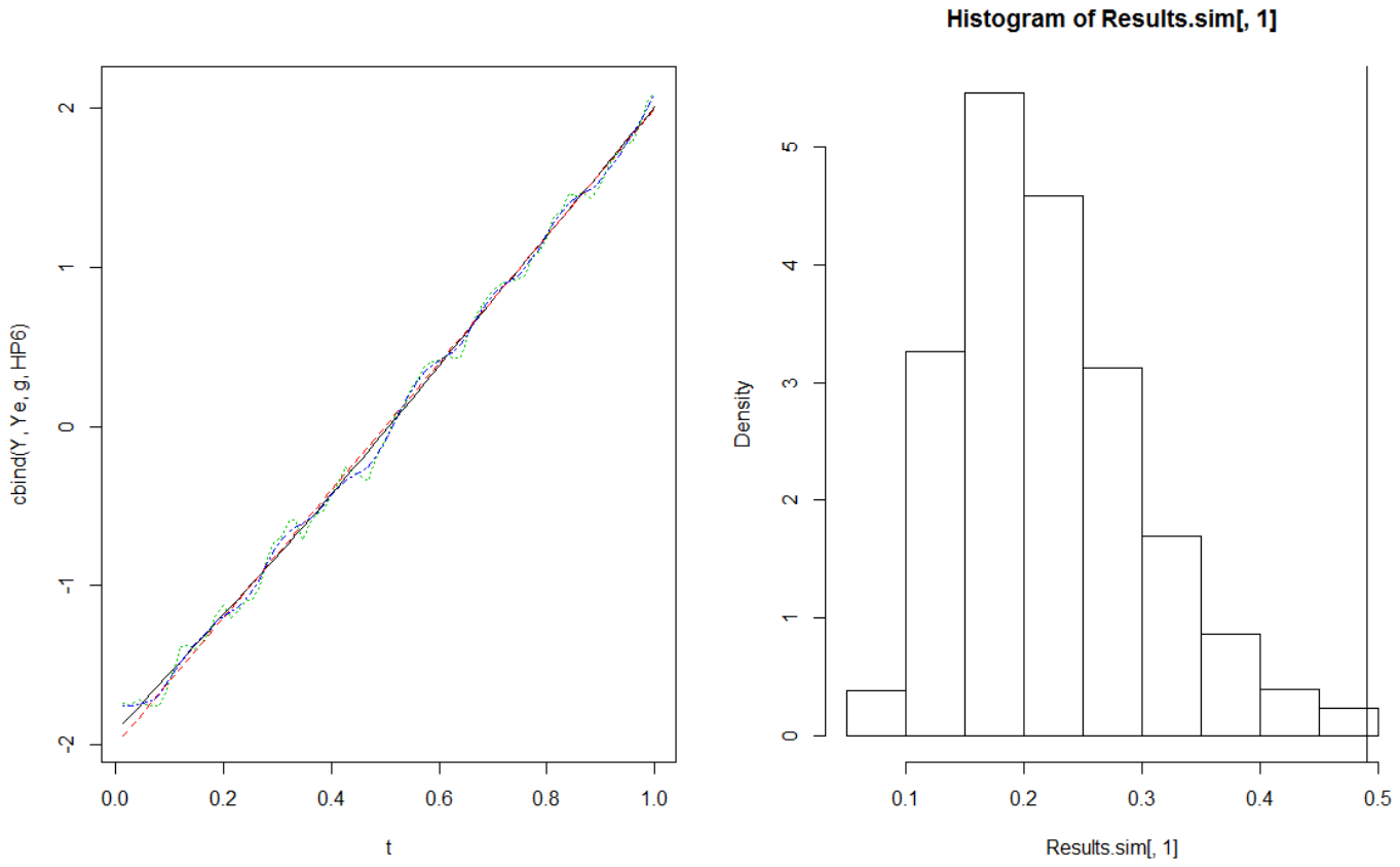
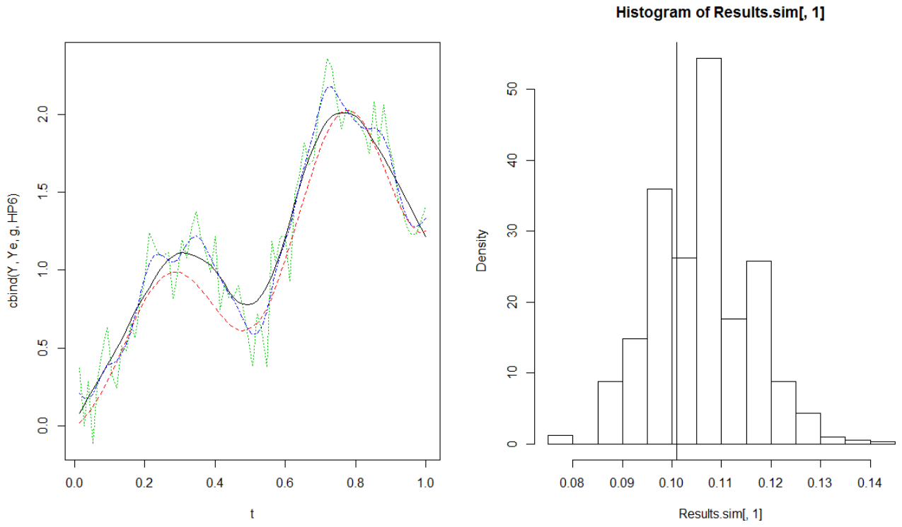
Obviously, the HP trend heavily depends on the smoothing parameter and the variance of the residual component, which can be detected by comparing the MSE values of different $\lambda$. Thus, sometimes the HP filter does not detect the underlying trend model correctly, and the estimated trend reflects some cyclical variations. This is especially visible in the left column of Figure 1, where $n=75$, ME = 1, and the true DGP is linear $g_1$ (red dashed). In these cases, the HP filter, with the “optimal” smoothing parameter selected by [13], attributes some cyclical fluctuations to the estimated HP trend (blue dotted), although they come from the cyclical process (green dotted). However, the local linear trend (black) is able to detect the true DGP and is quite similar to the simple linear trend, which is, as expected, the best model for this DGP. Nevertheless, the linear trend is only a special case for the underlying growth process of macroeconomic variables, although it is, in accordance with [45], a reasonable first approximation for some advanced economies. It is important to mention that the bandwidth selection across 1000 replications is asymptotically normal, as seen in Figure 1. Hence, the IPI algorithm works well in our simulated cases. Nevertheless, the theoretical optimal bandwidth cannot be calculated using Equation (6) for a linear DGP, because the second derivative of $m\left(x\right)$ does not exist (is zero).

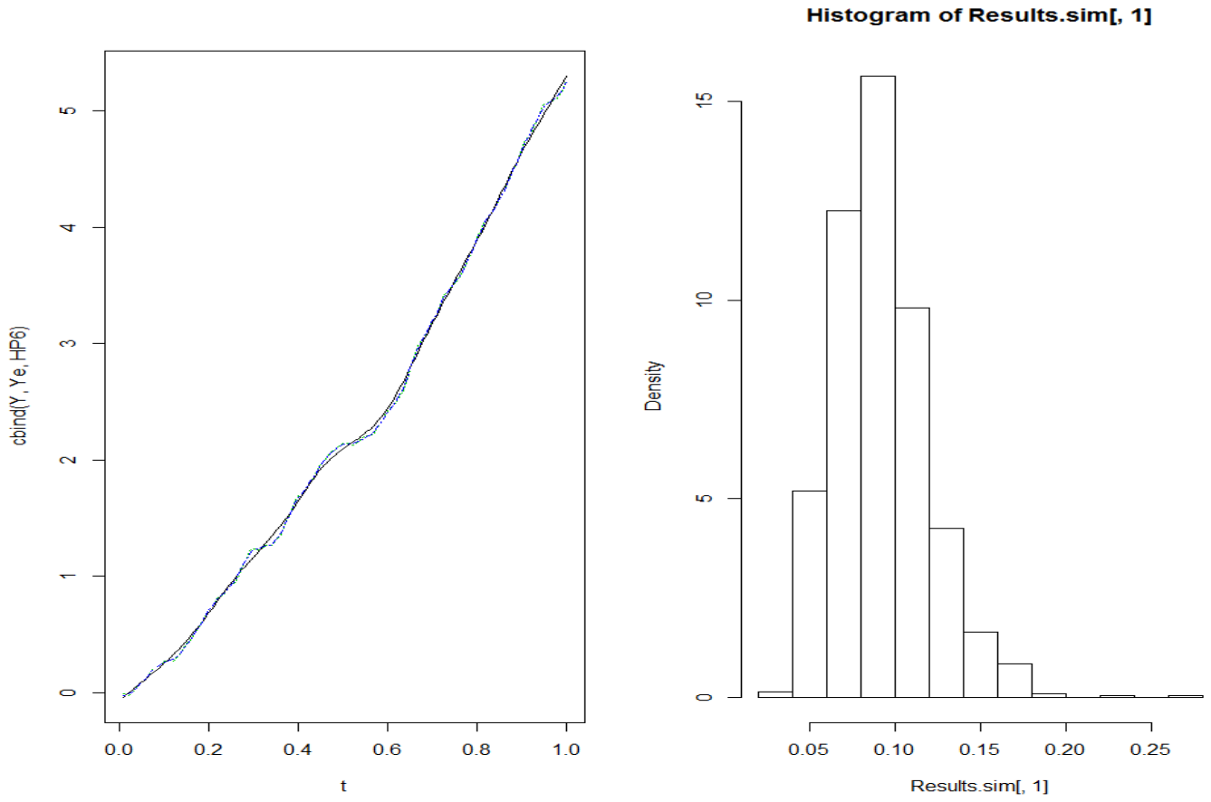
However, the growth path of developing economies, which usually displays a catching-up growth pattern, looks economically more interesting. In this case, the DGP is more likely to look like the red dashed process for $n=150$, ME = 1 in the left column of Figure 2. Again, the local linear trend (black) matches the true trend almost exactly. By contrast, the HP trend with $\lambda =6.25$ (blue dotted) is distorted by the cyclical process (green dashed), especially at the beginning and end of the series. Hence, the HP filter attributes too much of the cyclical fluctuations to the estimated trend function. This explains the spurious cycle phenomenon that is favored by “powerful low-frequency components … [not] impeded by the filter” ([6], p. 318). Furthermore, Figure 2 displays the distortion of the HP trend at the right boundary. The estimated HP trend is too low compared to the true DGP and the trend estimates of the local linear regression. This implies policy responses that may not be reliable. Interestingly, Hodrick [18] shows that the HP and Baxter and King [9] filters are superior to the Hamilton filter for slowly moving growth trends. Thus, our LLR could further improve the advantages of the HP filter for macroeconomic processes.

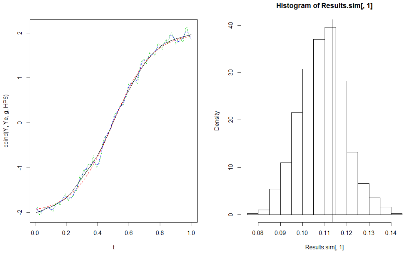
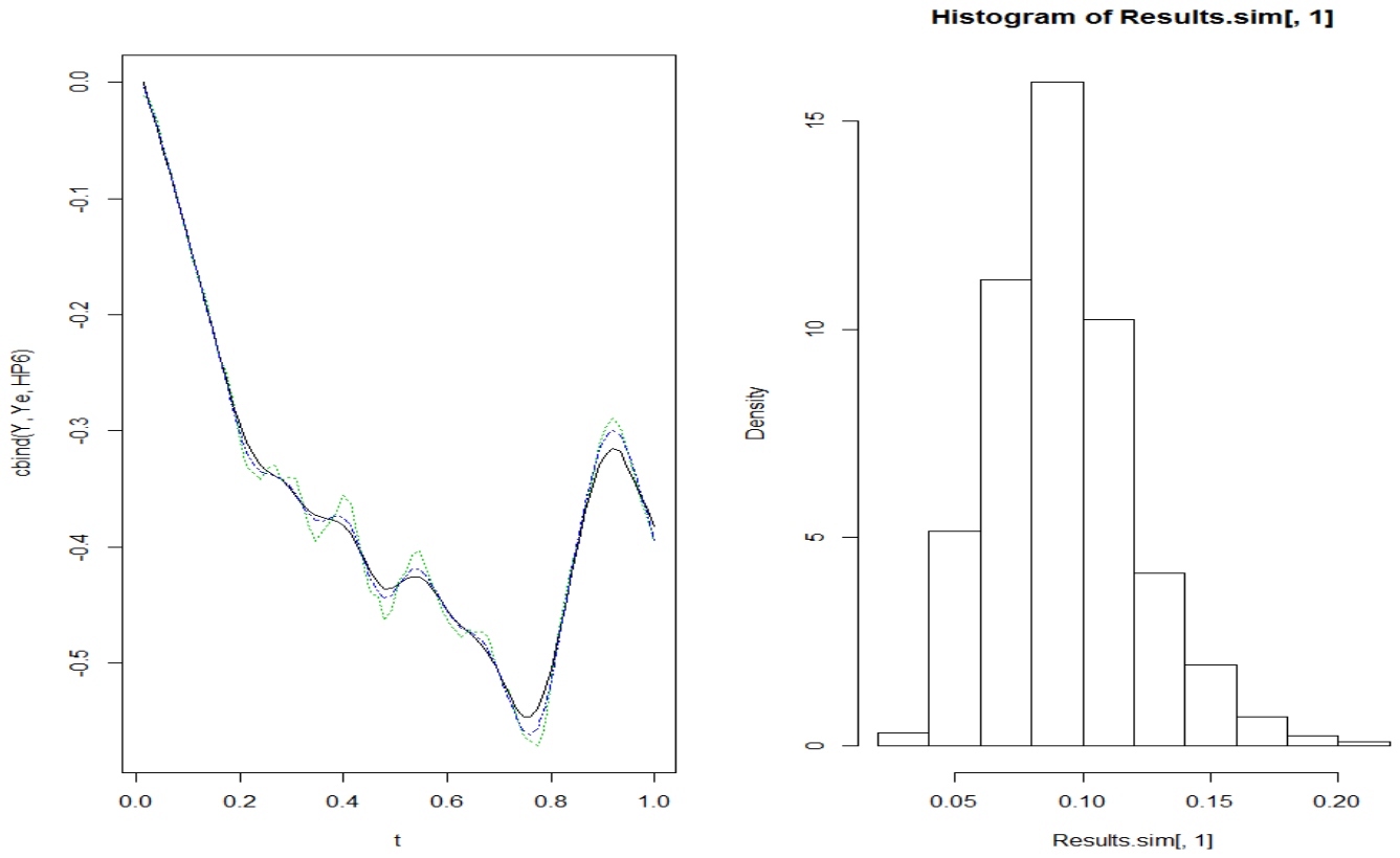
The right column shows the histogram of the selected bandwidths in 1000 repetitions. Compared to the theoretically correct bandwidth (black vertical line), the IPI algorithm for bandwidth selection works well in practice.

The results slightly change in Figure 3, where the complexity of the trend increases and the variance structure (ME = 2) changes. Obviously, the error process (green dotted) influences the trend estimation for the local linear and the HP trend. While the local linear trend (black solid) only reflects a biased trend level during the first peak, the error process dramatically drives the HP filter. In contrast to our approach, the HP filter (blue dot-dashed) does not detect the underlying true DGP, and its estimated trend again reflects some cyclical fluctuations. This also becomes obvious in Table A2, where the results with increased error-model variance favor the use of the LLR compared to the HP filter more strongly due to higher differences in the respective MSE values.

In accordance with [18], some economists argue that it is unlikely for slowly moving DGPs to behave like a Random Walk model; however, even when the trend follows a random walk without drift, with constant drift, or with linear drift, the local linear estimation approach is able to detect the DGP. This can be exemplarily seen from a random walk without drift (green dot-dashed) with $n=75$ in Figure A1 and a random walk with linear drift (green dot-dashed) with $n=150$ in Figure A2 in the Appendix A. Consequently, the proposed LLR method yields robust results by detecting the underlying DGP and the cyclical process. However, in such cases, our approach must be applied to the first differences in the series. Thus, a unit root test first needs to be carried out for the residual series obtained with the local linear approach. Secondly, in the case of a DS time series, our approach can be applied to the first differences of the series, and the trend can be estimated with the same IPI algorithm as in the TS case. In accordance with [24], it is important to note that “the application of a unit root test directly to a TS process without estimating and removing the trend properly is misleading, because the deterministic trend will usually be wrongly detected as a (spurious) unit-root” ([24], p. 69). It is important to mention that the HP filter does not work adequately when the trend is a random walk ([22], p. 15) and that stylized facts about comovement and periodicity display many movements implied by the HP filter. Reference [18] shows that for such simple random walk models, the Hamilton filter could be an interesting alternative. However, he also finds that for more complex models, the Hamilton filter does not work well. For detailed results of the discussion on TS and DS time series, see [24,41]. To sum up the results of the simulation study, the HP filter is not suitable for the analysis of long-term trends, as it frequently attributes too much cyclical variation to the estimated trend function and depends highly on the smoothing parameter. Moreover, the difficulties of the estimation of boundary points become visible.

5. Comparing Local Linear Trend and HP Trend: Real Data

In order to demonstrate the advantages of the local linear trend estimation with real data, the local linear and the HP trend are compared for different macroeconomic variables at different frequencies using US GDP data at a quarterly frequency covering the period from 1947.1 to 2016.1 and at an annual frequency covering the period from 1790 to 2015. The quarterly data are extracted from [46], and the annual data are from [47]. Moreover, we use far higher-frequency monthly data, namely the US dollar-British pound exchange rate from 01.1971 to 11.2017, extracted from [48].

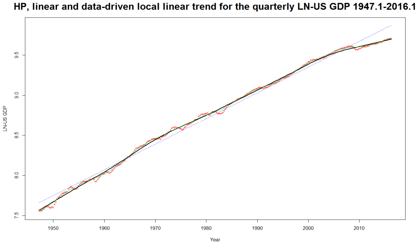
Figure 4 shows the quarterly US GDP data (red dots) together with the linear trend (blue dotted), the HP trend for $\mathit{\lambda }=\mathbf{1600}$ (green thin solid) and the local linear trend (black thick solid) for the endogenously determined bandwidth of 16 years ($\mathit{h}=\mathbf{0.1119}$). Figure 4 confirms [45] results involving approximately linear movements in some macroeconomic variables of advanced economies. 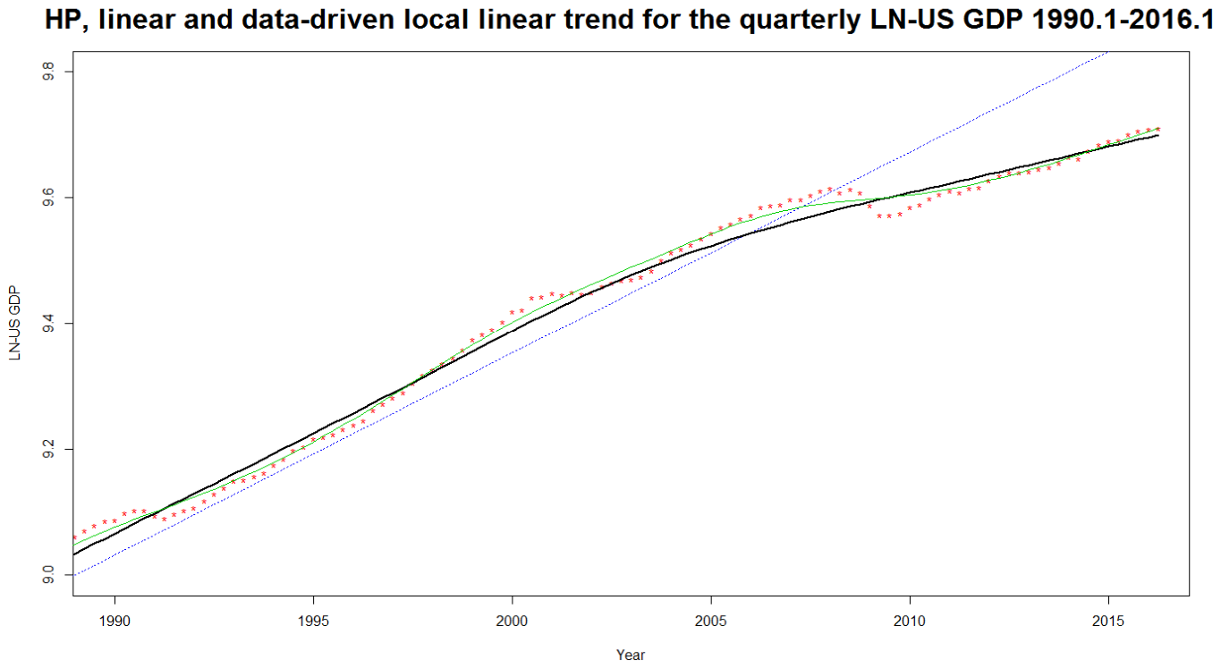Figure 5 displays the same results, zoomed in on the period from 1990.1 to 2016.1.

As can be seen from Figure 5, some major differences for the trends at the boundary points exist in the sense that our local linear trend is more stable and not as sensitive as the HP trend. The stability of our local linear approach is a necessary requirement for long-term growth trends that should not display any cyclical movements [22]. Nevertheless, the trend must reflect the general tendency of the economy. This general direction of economic development is depicted by the local linear trend, which, for example, shows higher growth rates during the golden age after the Second World War. Hence, the proposed method is able to reflect important events in economic history, is broadly consistent with growth drivers, and is related to potential economic theories. As each local linear trend is estimated through an endogenously chosen, stationary growth period, we also identify a trend-relevant growth period. This combination of growth trend and growth trend-period allows for a beneficial interpretation: a growth trend is economically explained by a (log-) linear growth model that relates empirically to the identified growth period. Trends are explained by theories that use long-term determinants to explain growth. However, if there are gradual changes in fundamental determinants, these changes also gradually change the growth rates. With this identified moving growth trend from empirical data, our approach corresponds to the moving changes in growth conditions.

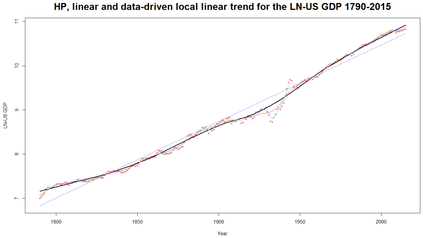
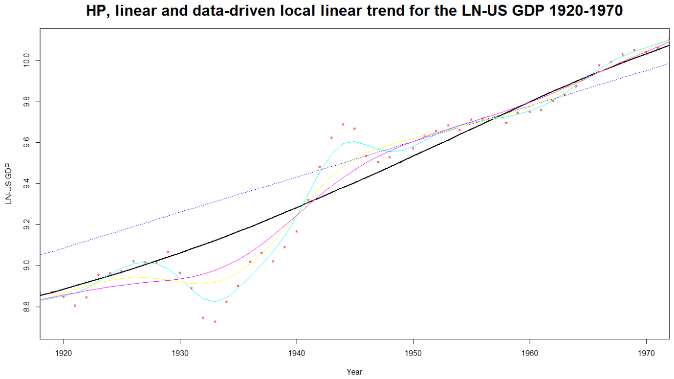
Figure 4 and Figure 5 demonstrate the problems associated with the HP trend for the usually considered quarterly data. However, whereas selecting the smoothing parameter for quarterly data with $\mathit{\lambda }=\mathbf{1600}$ is more or less common sense, adjusting this parameter for other frequencies is less consistent. Figure 6 shows the annual data (red dots) together with the linear trend (blue dotted), the HP trend for $\mathit{\lambda }=\mathbf{6.25}$ (turquoise thin solid), $\mathit{\lambda }=\mathbf{100}$ (yellow thin solid), $\mathit{\lambda }=\mathbf{400}$ (pink thin solid), and the local linear trend (black thick solid) with a relative bandwidth $\mathit{h}=\mathbf{0.1206}$. In other words, it presents different values for the smoothing parameter $\mathit{\lambda }$, ranging from the smallest to the highest values suggested in the literature, proposed by [13,28,34]. Again, Figure 6 demonstrates the same results zooming into the period from 1920 to 1970.

The HP trend obviously strongly depends on the arbitrarily selected $\mathit{\lambda }$. As a result, the extracted cycle highly depends on the smoothing parameter and is therefore also arbitrarily extracted. However, this paper focuses on the estimation of the trend component, with the analysis of the residual component going far beyond the scope of the paper. An example of cyclical analysis using the LLR is shown in [24]. From Figure 6 and Figure 7, it is obvious that the proposed method and the HP filter with $\mathit{\lambda }=\mathbf{400}$ [34] could yield quite similar trends, in the sense that our trend estimation results are in line with the method used most frequently by [7], if $\mathit{\lambda }$ for the HP filter is chosen appropriately. The corresponding cyclical components could also be quite similar. Yet, as can be seen from Figure 7, there are major differences for the trends from 1925 to 1950, where the local linear trend is smoother and more robust against outliers than the HP trend. This period comprises the Great Depression of the 1930s, which [49] analyzes using the HP filter. Reference [49] concludes that the HP trend follows the observation of GDP too closely and, accordingly, excludes the effects of the Great Depression from the cycle and attributes them to the estimated HP trend. Consequently, the Great Depression was portrayed less severely using the HP procedure than it actually was. As can be seen by the Great Depression and the Financial Crisis, the LLR method is (compared to the HP filter) robust in cases of sudden and extremely non-standard shocks. This is caused by the IPI algorithm and the kernel functions used. Thus, the proposed method is also robust during the COVID-19 pandemic, and the actual oil price shocks are. In other words, the bandwidth selection is only influenced if the shock is permanent, as can be detected in Figure 4 and Figure 5.

Thus, given our MT and the results from [49], $\mathit{\lambda }$ needs to be larger than usually suggested in the literature. Our results are in line with [22], who requires higher values of $\mathit{\lambda }$ because low values yield trends that overestimate the trend component and are too sensitive to cyclical fluctuations. Higher values of $\mathit{\lambda }$ can improve the relative efficiency of the HP filter. Arbitrarily selected values of the smoothing parameter result in a mixture of trend and cyclical movements, and cause ambiguous stylized facts about trends and business cycles. Furthermore, the wrong smoothing parameter yields different values for the output gap, which could be—in accordance with [50]—either negative or positive, highly depending on the selected $\mathit{\lambda }$.

Besides that, a main advantage of the local linear trend is the economic interpretation of the trend with the endogenously selected bandwidth as a Moving Trend MT. There are periods of continuous growth-trend segments arguing in favor of moving steady states, in contrast to a single overall steady-state growth process. Consequently, economic conditions change smoothly over the observation period. This directly corresponds to the log-linear growth models often discussed in growth theory. This local linear MT allows for a direct connection to theoretical interpretations. In other words, the proposed method is theoretically reasoned and statistically justified. This is also in line with the economically reasoned idea of [7]. The HP filter rests on the assumption that the decomposition needs to be supported by economic theory.

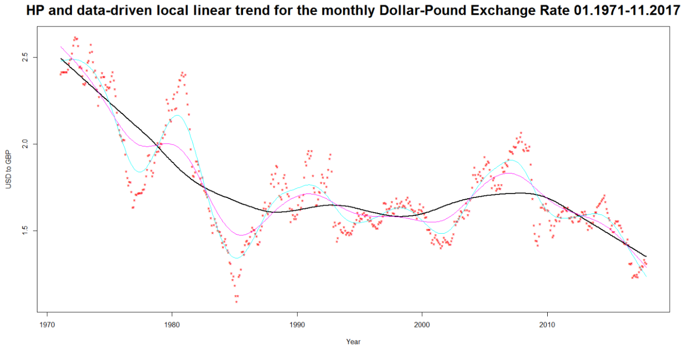
In order to demonstrate the wide range of applications for the local linear trend estimation approach, we apply it to some data other than the usually handled macroeconomic aggregates. Therefore, the US dollar-British pound exchange rate from January 1971 to November 2017 is shown in Figure 8, where the local linear regression (black thick solid) with a relative bandwidth $\mathit{h}=\mathbf{0.1515}$ is compared to the HP trend with λ = 14,400 (turquoise thin solid), suggested by [7] and in accordance with [13]’s λ = 129,600 (pink thin solid) for monthly data. It is important to note that the exchange rate is observed monthly and that the volatility of the smoothing parameter proposals is higher than in the annual case. Moreover, the exchange rate is far more volatile than GDP data and exhibits more pronounced upward and downward trend movements than macroeconomic aggregates. This more complex pattern is reflected within the data-driven local linear trend, which is able to capture all trend movements without reflecting cyclical behavior. By contrast, the HP trend, again depending heavily on the wide range of possible smoothing parameters, in the sense of [10], creates spurious effects, because many more cyclical fluctuations are attributed to the estimated trend function. This flexibility of the HP trend can again be penalized by higher values of the smoothing parameter.

In addition, Figure 8 demonstrates the poor behavior of the HP trend at boundary points as noted in [40]. This reaction stems from its non-causality and lack of adjustment near the boundary, a typical problem for unadjusted two-sided filters. Furthermore, Figure 8 displays the improvements in the local linear trend at these boundary points. Consequently, the estimated trend is much more stable at those points. It becomes clear why the output gap, calculated with the HP filter and different values of $\mathit{\lambda }$, needs to be interpreted with caution [51]. The implications for monetary policy following the output gap calculation using the HP filter need to be handled carefully, because they depend heavily on the HP specification used. Therefore, the local linear approach could be a better alternative for stabilizing the estimates of the output gap since it is compatible with economic theory. In accordance with [52] and the improvements at boundary points using the local linear method, a comparison to production function approaches for estimating the output gap is interesting for policy relevance. Moreover, this could be an interesting policy field for further application of the proposed method. In particular, improvements at boundary points are able to enhance estimation quality and, consequently, policy advice in order to boost growth. In line with [52], a production function approach uses capital, factor productivity, and labor, which are related to a level of capacity. Using a production function requires the specification of a functional form (e.g., Cobb–Douglas) and a world with perfect competition. Due to these exogenous parameter choices and the difference in both methods, a comparison is left for future research.

To sum up, the proposed data-driven local linear estimation method is able to handle different economic data sets as well as different frequencies (annual, quarterly, and monthly). It is important to note that, in accordance with [53], this approach is also able to handle daily and even higher frequencies. Moreover, a reliable trend is estimated endogenously and justified theoretically.

6. Conclusions

This paper suggests an alternative, nonparametric, flexible method for trend and cycle decomposition, in particular compared to the widely used HP filter. First, the HP trend and its drawbacks are presented as a standard benchmark. Second, we explain our nonparametric estimation approach. We suggest an IPI algorithm for local linear regression (LLR) with endogenous bandwidth selection based on the MSE. Third,—and this is our main focus—we illustrate why we regard this new procedure as a superior substitute for the most widely used HP filter. Therefore, besides a detailed simulation study, real US GDP and exchange rate data demonstrate the usefulness of the local linear approach for trend estimation. The simulation study shows that the local linear trend is able to detect the true DGP, whereas the performance of the HP trend highly depends on the smoothing parameter and the error dependence structure. The comparison of our approach and the HP trend displays that the trend curves become similar for proper choices of $\lambda$, which needs to be several times higher than the inverse signal-to-noise ratio. Thus, our local linear trend improves the main disadvantages of the HP filter, such as the arbitrary selection of $\lambda$ its poor behavior at boundary points and the independent errors assumption. Moreover, selecting the bandwidth data-driven requires fewer exogenous parameter choices for an optimal trend and cycle decomposition. The interpretation of continuously moving trend (MT) processes, which last around 16 years for postwar quarterly GDP data, reflects economic growth dynamics. Economically, these periods may represent stable macroeconomic decision-making segments. Hence, the more flexible local linear trend estimation could be a preferred method, as it refines some drawbacks of the HP trend and directly relates to log-linear growth theories. Its simplicity and extensive application possibilities could make it the successor of the limited HP filter. It is left for future research to compare the asymptotic properties of both filtering methods in greater detail, to analyze their effects on business cycle and output gap estimation, and to compare their forecasting ability.