Article

HAGWO: A Hierarchical Adversarial Grey Wolf Optimizer and Its Application in the 3D Bin Packing Problem

Computer Engineering College, Jimei University, Xiamen 361021, China
*
Authors to whom correspondence should be addressed.
Mathematics 2026, 14(16), 3011; https://doi.org/10.3390/math14163011
Submission received: 29 May 2026 / Revised: 1 August 2026 / Accepted: 10 August 2026 / Published: 20 August 2026

Abstract

The Grey Wolf Optimizer (GWO) is a popular metaheuristic, yet it often suffers from premature convergence and rapid diversity loss in complex, high-dimensional, or highly constrained optimization problems. This paper introduces HAGWO, a novel Hierarchical Adversarial Grey Wolf Optimizer that addresses these limitations through three synergistic enhancements: dynamic hierarchical population stratification, adaptive Levy flight perturbation, and hierarchical adversarial-like position updating. These mechanisms enable adaptive balancing of global exploration and local exploitation while preserving population diversity throughout the search process. Extensive experiments on the CEC 2017 bound-constrained benchmark suite across 30D, 50D, and 100D dimensions demonstrate that HAGWO achieves superior overall performance among eight state-of-the-art algorithms, with statistically significant advantages confirmed by Friedman mean ranks and Wilcoxon signed-rank tests. When adapted to the strongly NP-hard three-dimensional bin packing problem with identical bins (3D-SBSBPP), HAGWO delivers highly competitive results, outperforming the well-established BRKGA and most other metaheuristics while closely approaching the original GWO in solution quality and exhibiting exceptional run-to-run stability. By rigorously evaluating HAGWO across both high-dimensional continuous benchmarks and a practical constrained combinatorial application, this study validates the effectiveness of its hierarchical adversarial-like framework and provides valuable insights into algorithm design and transferability across different problem domains.

1. Introduction

Optimization problems permeate science, engineering, and industry, ranging from continuous parameter tuning to discrete combinatorial decision-making. Among these, high-dimensional continuous optimization [1] and strongly constrained combinatorial tasks—such as the three-dimensional bin packing problem (3D-BPP)—remain particularly challenging due to multimodal landscapes, the curse of dimensionality, and strict feasibility constraints [2]. While exact methods are often intractable for large-scale instances, metaheuristic algorithms, especially swarm intelligence (SI) techniques inspired by collective natural behaviors, have emerged as powerful tools for efficiently navigating complex search spaces.
Over recent decades, numerous SI algorithms have been developed, including Particle Swarm Optimization (PSO) [3], Differential Evolution (DE) [4], Artificial Bee Colony (ABC) [5], and Whale Optimization Algorithm (WOA) [6]. These methods have achieved considerable success across diverse applications. Nevertheless, many still suffer from premature convergence, rapid loss of population diversity, and inadequate exploration–exploitation balance, particularly in high-dimensional or highly constrained scenarios [7,8,9].
The Grey Wolf Optimizer (GWO), introduced by Mirjalili et al. [10], is among the most widely adopted SI algorithms. Drawing inspiration from the social hunting hierarchy of grey wolves, GWO assigns leadership roles to alpha, beta, and delta wolves, with omega wolves updating positions based on these leaders. Its simplicity, minimal parameter tuning, and strong global search capability have led to successful applications in both continuous and discrete problems [11]. However, the original GWO exhibits notable limitations: (1) premature convergence and diversity loss in later stages, especially on multimodal or high-dimensional landscapes; (2) a rigid, uniform update strategy guided solely by the top three leaders, limiting phase-specific adaptability; and (3) reduced flexibility in highly constrained combinatorial problems such as 3D-BPP, where geometric and capacity constraints demand more nuanced local adjustments.
To address these shortcomings, this paper proposes HAGWO (Hierarchical Adversarial Grey Wolf Optimizer), a novel enhancement of GWO incorporating three synergistic innovations: (1) dynamic hierarchical population stratification, inspired by concepts such as Tianji’s horse racing optimization [12], which adaptively partitions the population into superior, medium, and inferior groups with evolving proportions across search phases; (2) hierarchical adversarial-like position updating, assigning distinct update rules to each group to foster opposition-based learning and directed information flow; and (3) an adaptive Levy flight perturbation mechanism that provides controlled long-range exploration with intensity decreasing over iterations [13]. The term “adversarial” in HAGWO refers to an opposition-based perturbation strategy inspired by adversarial learning principles, rather than a game-theoretic minimax formulation.
The effectiveness of HAGWO is rigorously validated through two complementary experimental tracks. On the CEC 2017 benchmark suite [1] in 30D, 50D, and 100D dimensions, HAGWO achieves superior overall performance among eight state-of-the-art algorithms, with statistical significance confirmed by Friedman and Wilcoxon rank-sum tests. When adapted to the strongly NP-hard three-dimensional single-bin-size bin packing problem (3D-SBSBPP), HAGWO delivers highly competitive results, outperforming the established BRKGA [14] and several other metaheuristics while achieving the second-best overall performance in terms of total bin count and exhibiting exceptional run-to-run stability.
The main contributions of this study are as follows:
  • We propose HAGWO, an effective GWO variant that integrates dynamic hierarchical stratification, adversarial-like position updating, and adaptive Levy flight perturbation to enhance diversity, adaptability, and search efficiency.
  • We conduct comprehensive high-dimensional benchmarking on CEC 2017, demonstrating statistically significant superiority in continuous optimization.
  • We adapt HAGWO to 3D-SBSBPP and provide a detailed comparative analysis, offering insights into algorithm transferability across continuous benchmarks and constrained combinatorial applications.
The remainder of the paper is organized as follows. Section 2 reviews related work. Section 3 details the proposed HAGWO algorithm. Section 4 describes its adaptation to 3D-BPP. Section 5 presents the experimental setup and results. Section 6 discusses key findings, implications, and limitations. Finally, Section 7 concludes the paper.

2. Related Work

SI algorithms have emerged as powerful tools for solving complex optimization problems, drawing inspiration from natural collective behaviors. Among them, GWO [10] has gained significant attention due to its intuitive social hierarchy and strong global search capabilities. The algorithm’s explicit division into alpha, beta, delta, and omega wolves provides a natural structural substrate for tiered extensions, making it particularly amenable to enhancements that require role-differentiated update strategies. However, the original GWO often suffers from premature convergence in high-dimensional or multimodal landscapes [11].
To enhance GWO’s performance, numerous variants have been proposed. Nadimi-Shahraki et al. [11] introduced the Improved Grey Wolf Optimizer (I-GWO), which incorporates a dimension learning-based hunting (DLH) search strategy to enhance both global and local search capabilities; it was evaluated on the CEC 2018 benchmark suite and demonstrated strong competitiveness. Jiang et al. [15] proposed the Enhanced GWO with Elite Inheritance and Balance Search Mechanisms (EBGWO), which inherits elite solutions across generations and stochastically balances exploration and exploitation. More recent advancements include the Improved Adaptive GWO (IAGWO) that employs multi-strategy ensemble and adaptive mechanisms to significantly enhance exploration [9], and the Scale-Free Network-based GWO (SFGWO), which divides the population into network-structured layers [16]. Hybrid strategies have also been introduced, such as the Genetic Learning-based Grey Wolf Optimizer (GL-GWO) [17]. Despite these advances, few studies have focused on hierarchical adversarial-like enhancements of GWO on the CEC 2017 suite, and their efficacy in constrained combinatorial problems remains underexplored.
The CEC 2017 benchmark suite [1] is a standard testbed for evaluating metaheuristics on single-objective real-parameter optimization. It includes 30 functions categorized into unimodal, multimodal, hybrid, and composition types. Several SI algorithms, including CCO [18], WOA [6], and EAO [19], have been benchmarked on CEC 2017, with statistical tests like Friedman and Wilcoxon being used to validate significance [20].
In the domain of combinatorial optimization, the three-dimensional bin packing problem (3D-BPP) [2] is a classic NP-hard problem with significant applications in logistics, manufacturing, and supply chain management. The objective is to pack a set of rectangular items into a minimum number of identical rectangular bins while respecting constraints such as item orientations, non-overlapping placements, and stability requirements. Unlike its two-dimensional counterpart, 3D BPP introduces additional complexity due to the need for three-dimensional spatial reasoning and rotation possibilities (up to six orientations per item), making exact methods computationally infeasible for large instances [21].
Heuristic and metaheuristic approaches have been extensively explored to tackle 3D BPP. Traditional heuristics include the First-Fit Decreasing (FFD) and Best-Fit Decreasing (BFD) strategies, often combined with space-filling rules like the Lowest Bottom-Left (LBL) or Extreme Point-Based Space (EMS) [22]. Metaheuristics enhance these heuristics by providing global search capabilities. For example, Genetic Algorithms (GAs) have been adapted with biased random-key encodings in BRKGA [14], which decodes chromosomes into item sequences and orientations for effective packing. The Grey Wolf Optimizer (GWO) [10] has been applied to packing problems with notable success [11]. However, advanced modifications incorporating hierarchical or adversarial-like mechanisms in GWO remain scarce for 3D BPP. This study bridges these gaps by proposing HAGWO and evaluating it on both CEC 2017 and 3D BPP.

3. Proposed HAGWO

The proposed Hierarchical Adversarial Grey Wolf Optimizer (HAGWO) builds upon the foundational principles of the original GWO while addressing its key limitations through novel enhancements. In this section, we first provide an overview of the original GWO algorithm and analyze its shortcomings, followed by a detailed description of HAGWO’s three synergistic innovations: dynamic hierarchical population stratification, adaptive Levy flight perturbation mechanism, and hierarchical adversarial-like position updating.

3.1. Original Grey Wolf Optimizer (GWO)

The Grey Wolf Optimizer (GWO), introduced by Mirjalili et al. [10], is a metaheuristic inspired by the social hunting hierarchy and behavior of grey wolves. The algorithm divides the wolf pack into four levels: alpha ( α ) as the leader, beta ( β ) as the second-in-command, delta ( δ ) as the third, and omega ( ω ) as the followers. The search process mimics encircling, hunting, and attacking prey.
The encircling behavior is modeled as
D = | C · X p ( t ) X ( t ) | ,
where X p ( t ) represents the prey position (approximated by α , β , or δ ), X ( t ) is the current wolf position, and C is a coefficient vector that adds randomness to the encircling.
The position update is given by
X ( t + 1 ) = X p ( t ) A · D ,
where A controls the step size and direction, allowing for both exploration (when | A | > 1 ) and exploitation (when | A | < 1 ).
The coefficients are defined as
A = 2 a · r 1 a ,
C = 2 · r 2 ,
with a linearly decreasing from 2 to 0 over iterations to transition from exploration to exploitation, and r 1 , r 2 being random vectors in [0, 1] for stochasticity.
The hunting phase averages the positions guided by the top three wolves:
X ( t + 1 ) = X 1 + X 2 + X 3 3 ,
where X 1 , X 2 , and X 3 are positions updated toward α , β , and δ , respectively. The pseudocode of GWO is presented in Algorithm 1.
Algorithm 1 Pseudocode of the Original GWO.
Require: Population size N, maximum iterations T max , dimension d i m , bounds l b , u b
Ensure: Optimal solution X best , fitness f ( X best )
 1:
Initialize population X and evaluate fitness
 2:
Identify α , β , δ
 3:
for  t = 1 to T max  do
 4:
    Update a = 2 2 × ( t / T max )
 5:
    for each wolf i do
 6:
        Compute X 1 , X 2 , X 3 with Equations (1) and (2) toward α , β , δ
 7:
        Update X ( i , : ) using Equation (5)
 8:
        Apply boundary handling
 9:
    end for
10:
    Reevaluate fitness and update α , β , δ
11:
end for
12:
Return X best , f ( X best )

3.2. Limitations of Original GWO

Despite its effectiveness, the original GWO exhibits several limitations, particularly in complex optimization landscapes. First, the uniform update strategy for all wolves leads to rapid loss of population diversity, causing premature convergence in multimodal or high-dimensional problems [11]. Second, the fixed leadership hierarchy (relying solely on the top three wolves) lacks adaptability across different search phases, often resulting in insufficient exploration in the early stages and poor exploitation later on [23]. These issues motivate the development of enhanced variants that incorporate hierarchical structures, adversarial-like mechanisms, and advanced disturbance strategies.

3.3. HAGWO: Hierarchical Adversarial Grey Wolf Optimizer

To overcome the above limitations while leveraging the structural plasticity of GWO’s hierarchy, HAGWO introduces three synergistic enhancements: (1) dynamic hierarchical population stratification, (2) adaptive Levy flight perturbation mechanism, and (3) hierarchical adversarial-like position updating. These mechanisms work in concert to achieve adaptive balance between global exploration and local exploitation while maintaining population diversity throughout the search process. The population is dynamically stratified into superior ( ς ), medium ( ζ ), and inferior ( ξ ) groups based on fitness rankings.

3.3.1. Dynamic Hierarchical Population Stratification

HAGWO employs a dynamic hierarchical population stratification mechanism based on phase-aware search progression. The population is partitioned into superior ( ς ), medium ( ζ ), and inferior ( ξ ) groups according to fitness rankings. The group proportions adaptively evolve based on the search phase:
In the early phase ( t 0.5 × T max ), a larger proportion of inferior wolves promotes broad global exploration:
n ς = 0.1 × N n ζ = 0.3 × N n ξ = N n ς n ζ
In the late phase ( t > 0.5 × T max ), an increased share of superior wolves enhances focused local exploitation:
n ς = 0.3 × N n ζ = 0.3 × N n ξ = N n ς n ζ
Design rationale and parameter justification. The stratification ratios ( 0.1 ,   0.3 ,   0.6 ) in the early phase and ( 0.3 ,   0.3 ,   0.4 ) in the late phase are determined by the following design principles. First, the medium group ratio is fixed at 0.3 to ensure a stable transitional layer between superior and inferior wolves throughout the optimization process. Second, in the early phase, the superior ratio of 0.1 ensures that at least one elite wolf exists for any population size N 10 , while the remaining 0.6 inferior wolves maximize exploration coverage. In the late phase, the superior ratio increases to 0.3 to intensify exploitation around promising regions, while the inferior ratio decreases to 0.4 to maintain residual diversity. The threshold at 0.5 × T max represents a standard phase transition point that balances early exploration and late exploitation, consistent with established practices in phase-aware metaheuristic design [9,16]. We acknowledge that these ratios constitute a manually designed schedule rather than a fully adaptive fuzzy mechanism; the term “phase-aware” is used to describe this deliberate phase-dependent structural control.

3.3.2. Adaptive Levy Flight Perturbation Mechanism

To augment the algorithm’s capability to escape local optima and enhance long-range exploration, HAGWO integrates an adaptive Levy flight perturbation mechanism. The disturbance factor is formulated as
d f = 0.1 × p × Levy ( λ ) , λ = 1.5 ,
where p = 1 t / T max serves as a linearly decreasing scaling coefficient, ensuring stronger perturbation in early-to-mid stages (promoting diversity via long jumps) and gradual attenuation in later stages (supporting precise local refinement).
The Levy flight step Levy ( λ ) is generated using the Mantegna algorithm [24]:
L = u | v | 1 / λ , u N ( 0 , σ u 2 ) , v N ( 0 , 1 ) ,
where
σ u = Γ ( 1 + λ ) sin ( π λ / 2 ) Γ ( ( 1 + λ ) / 2 ) λ 2 ( λ 1 ) / 2 1 / λ ,
and Γ ( · ) is the gamma function.
Parameter justification. The Levy flight exponent λ = 1.5 is adopted following established practice in Levy-enhanced swarm intelligence methods [25,26]. This value lies in the theoretically recommended range 1 < λ 3 and has been empirically validated across numerous metaheuristic algorithms including cuckoo search [26] and various GWO variants [27]. The scaling coefficient 0.1 in Equation (8) ensures that the disturbance magnitude remains a small fraction of the search space, preventing excessive disruption of promising solutions while providing sufficient perturbation to escape local optima. The linearly decreasing term p = 1 t / T max naturally attenuates the disturbance intensity as the search progresses, aligning with the widely accepted principle that exploration should dominate early and exploitation should dominate late [10]. These parameter choices require no additional problem-specific tuning beyond the standard GWO parameters.

3.3.3. Hierarchical Adversarial-like Position Updating

HAGWO implements hierarchical adversarial-like position updating, where each stratified group employs a distinct opposition-based strategy to drive competition and learning against higher-tier guidance. We clarify that the term “adversarial” herein refers to an opposition-based perturbation mechanism inspired by the concept of adversarial learning, rather than a game-theoretic minimax formulation or an explicit multi-objective adversarial game. Specifically, lower-tier wolves generate candidate positions by actively opposing the direction suggested by higher-tier guidance, creating reverse-search trajectories that enhance exploration. This mechanism ensures directed information flow from superior to inferior groups while actively opposing suboptimal directions through perturbation terms.
Let X ¯ = ( X α + X β + X δ ) / 3 denote the mean position of the current top three leaders. The group-specific candidate position update rules are as follows:
- Superior wolves ( ς ): focus on elite refinement and internal information exchange:
X ς , i = p · X ¯ + ( 1 p ) · X ς ( rand ) ,
where X ς ( rand ) is the position of a randomly selected superior wolf (different from the current individual).
- Medium wolves ( ζ ): integrate superior guidance with an adversarial-like perturbation scaled by the disturbance factor:
X ζ , i = p · X ¯ + ( 1 p ) · X ς ( rand 1 ) + d f · X ζ , i p · X ¯ + ( 1 p ) · X ς ( rand 2 ) ,
where X ς ( rand 1 ) and X ς ( rand 2 ) are independently sampled superior wolves. The perturbation term generates an opposition direction relative to a superior-guided position.
- Inferior wolves ( ξ ): perform aggressive opposition learning against medium wolves to drive global exploration:
X ξ , i = p · X ¯ + ( 1 p ) · X ζ ( rand 1 ) + X ζ ( rand 2 ) 2 + d f · p · X ¯ + ( 1 p ) · X ζ ( rand 1 ) + X ζ ( rand 2 ) 2 X ξ , i .
Once the candidate positions X · , i have been computed for all wolves, a boundary correction mechanism is executed to maintain feasibility. Subsequently, an elitist selection criterion is invoked: a newly generated position is adopted solely when it demonstrates superior or equivalent fitness compared with the incumbent; otherwise, the current position is preserved.
Component interaction and synergistic design. The three mechanisms in HAGWO are designed to function as an integrated system rather than independent modules. The dynamic stratification determines which wolves receive which update rules; the adversarial-like updating provides the directional structure for each group’s search behavior; and the Levy flight perturbation supplies the stochastic magnitude for exploration. Removing any single mechanism would break this structural coherence: without stratification, all wolves would use identical update rules, reverting to the original GWO’s uniform strategy; without the adversarial-like component, the stratified groups would lack directional opposition; and without Levy perturbation, the escape capability from local optima would be substantially weakened. Consequently, the synergistic interaction among the three components constitutes the core contribution of HAGWO. The individual contribution of each mechanism is empirically validated through the ablation study presented in Section 5.5.

3.3.4. Pseudocode

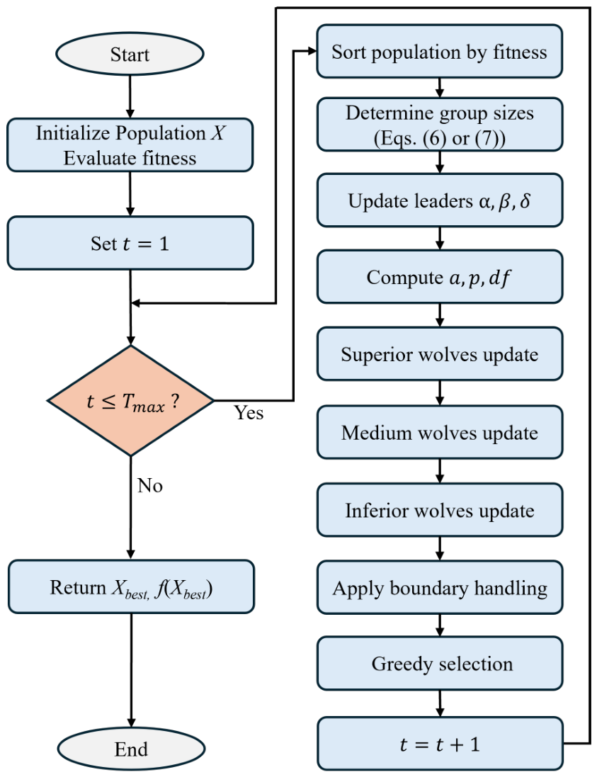
The complete pseudocode and flowchart of HAGWO are detailed in Algorithm 2 and Figure 1, respectively.
Algorithm 2 Pseudocode of the proposed HAGWO algorithm.
Require: Population size N, maximum iterations T max , dimension d i m , bounds l b , u b
Ensure: Optimal solution X best , fitness f ( X best )
 1:
Initialize population X and evaluate fitness
 2:
for  t = 1 to T max  do
 3:
    Sort population by fitness
 4:
    Determine group sizes based on Equations (6) or (7)
 5:
    Update leaders α , β , δ
 6:
    Compute a = 2 2 × ( t / T max )
 7:
    Compute p = 1 t / T max
 8:
    Compute d f = 0.1 × p × Levy ( λ )
 9:
    for each superior wolf do
10:
        Update using Equation (11)
11:
    end for
12:
    for each medium wolf do
13:
        Update using Equation (12)
14:
    end for
15:
    for each inferior wolf do
16:
        Update using Equation (13)
17:
    end for
18:
    Apply boundary handling and greedy selection
19:
end for
20:
Return X best , f ( X best )

3.4. Computational Complexity Analysis

We conduct a rigorous complexity analysis to investigate the computational implications of the proposed enhancements, directly comparing HAGWO against the original GWO. In what follows, N signifies the population size, D denotes the problem dimension, T max indicates the maximum iteration count, and f eval stands for the cost incurred by a single fitness evaluation.
Original GWO. In each iteration, GWO performs (i) fitness evaluation for all N wolves, costing O ( N · f eval ) ; (ii) sorting to identify α , β , δ , costing O ( N log N ) ; and (iii) position updates for all N wolves across D dimensions, costing O ( N · D ) . The total time complexity is therefore
O T max · ( N log N + N · D + N · f eval ) .
The space complexity is O ( N · D ) for storing the population matrix.
Proposed HAGWO. In each iteration, HAGWO additionally performs (i) dynamic stratification, which requires only index-based partitioning after sorting and thus adds O ( N ) —negligible compared to the O ( N log N ) sorting already required for leader identification; (ii) Levy flight generation via the Mantegna algorithm, which produces D random variates per wolf at O ( 1 ) per dimension, yielding O ( N · D ) ; and (iii) hierarchical adversarial-like updates, which compute candidate positions for all N wolves across D dimensions, also yielding O ( N · D ) . The greedy selection step evaluates one candidate position per wolf, adding O ( N · f eval ) , which is identical to the fitness re-evaluation cost already present in GWO. Consequently, the asymptotic time complexity of HAGWO remains
O T max · ( N log N + N · D + N · f eval ) ,
strictly of the same order as GWO. The space complexity is likewise unchanged at O ( N · D ) .
Practical runtime overhead. While HAGWO preserves the same asymptotic complexity as GWO, the practical per-iteration overhead includes Levy random number generation (Mantegna algorithm), subgroup assignment, and the additional arithmetic operations in the adversarial-like update equations. To quantify this overhead, we measured the average runtime per iteration for both GWO and HAGWO on the CEC 2017 F1 function at D = 30 dimensions with N = 30 wolves. The results show that HAGWO incurs approximately 8–12% additional runtime per iteration compared to GWO, primarily attributable to the Levy flight generation and the more complex position update calculations. For the 3D-BPP experiments, where fitness evaluation dominates the computational cost (due to the expensive DFTRC-2 placement heuristic), the relative overhead of HAGWO’s additional operations is less than 3% of the total execution time. These observations confirm that HAGWO’s enhanced search capabilities are achieved with only modest practical computational cost.

4. Adaptation of HAGWO to the 3D Bin Packing Problem

To investigate the generalization capability of HAGWO to discrete combinatorial optimization problems, we adapt it to the three-dimensional single-bin-size bin packing problem (3D-SBSBPP). The adaptation retains the core HAGWO evolutionary framework while integrating problem-specific encoding, decoding, and placement components to ensure packing feasibility and solution quality.

4.1. Problem Formulation: Three-Dimensional Single-Bin-Size Bin Packing

The three-dimensional single-bin-size bin packing problem (3D-SBSBPP) requires packing a set of n rectangular boxes, each with dimensions ( l i , w i , h i ) for i = 1 , , n , into the minimum number of identical rectangular bins of fixed dimensions ( L , W , H ) . All dimensions are positive integers, and without loss of generality, each box satisfies l i L , w i W , h i H after possible rotations. Boxes may be rotated in any of the six orthogonal orientations but must remain axis-aligned with the bin edges. No overlapping is allowed, and each box must lie completely within a bin.
The problem is strongly NP-hard [2] and has wide industrial applications, including container loading, palletizing, cargo arrangement, warehouse optimization, and arises as a subproblem in cutting, scheduling, and logistics planning [28,29].
Due to the combinatorial complexity and strong constraints, exact mixed-integer programming approaches become intractable for large instances. Instead, we adopt a metaheuristic approach based on biased random-key encoding and deterministic decoding, which guarantees feasible packings through a greedy placement heuristic while allowing efficient search in a continuous space.

4.2. Encoding and Decoding Framework

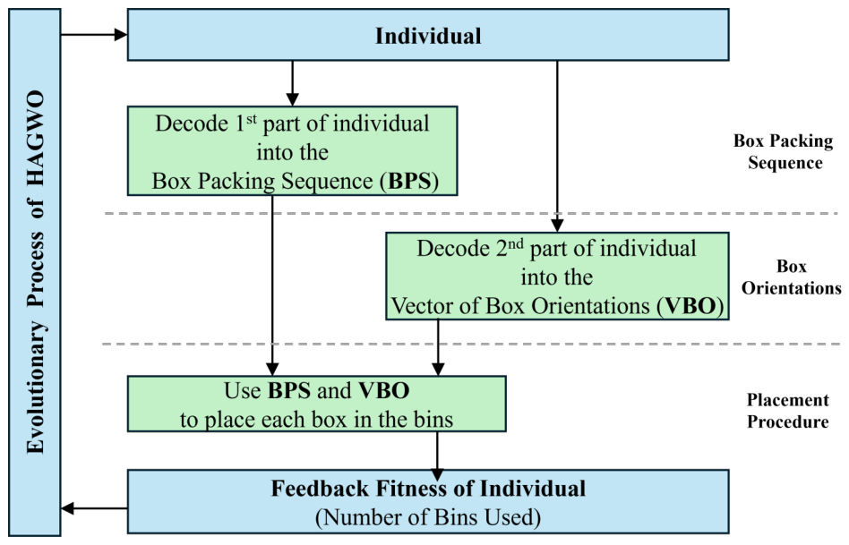
Each candidate solution in HAGWO is represented as a real-valued vector of length 2 n with components uniformly distributed in [ 0 ,   1 ] . The vector is semantically divided into two parts:
  • The first n keys encode the box packing sequence (BPS), i.e., the priority order in which boxes are considered for placement.
  • The second n keys encode the vector of box orientation biases (VBO), which guides biased selection of orientations during placement.
The decoding procedure transforms an individual into a feasible packing configuration in a deterministic manner:
  • Decoding of BPS: Sort the first n keys in ascending order to obtain permutation π . Then, BPS = [ π ( 1 ) , π ( 2 ) , , π ( n ) ] , where BPSi is the box index placed at stage i. Lower key values indicate higher placement priority.
  • Decoding of VBO: The second n keys directly form VBO = [ v 1 , , v n ] [ 0 , 1 ] n . For each box i in the BPS order, v i is used to select a biased orientation from the feasible set in the chosen maximal space.
  • Placement and feasibility: Boxes are placed sequentially using Algorithm 4. For each box, (1) attempt placement in existing bins using the DFTRC-2 heuristic (Algorithm 3); (2) if no feasible maximal space is found, open a new bin and place the box at the origin ( 0 , 0 , 0 ) ; and (3) update maximal spaces using the difference process (DP) [30] with added pruning rules for efficiency. The placement process guarantees no overlap, axis-alignment, and boundary compliance.
  • Fitness evaluation: After all boxes are placed, compute the number of used bins NB and the adjusted fitness value (detailed in Section 4.3.5).
This encoding–decoding framework ensures every individual produces a feasible solution, while HAGWO evolves high-quality sequences and orientation biases in the continuous space [ 0 ,   1 ] 2 n . Figure 2 illustrates the overall architecture of the proposed approach.

4.3. Common Components

The following components support the decoding and placement process, ensuring efficient and feasible packings.

4.3.1. Maximal-Space Representation

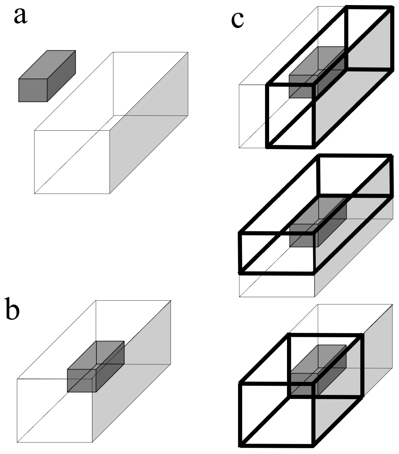
We adopt the maximal-space representation to track available empty spaces in bins, using a list S of empty maximal spaces (EMSs). Each EMS is defined by its minimum and maximum coordinates ( x i ,   y i ,   z i and X i ,   Y i ,   Z i ). To manage EMSs, we employ the difference process (DP) from Lai and Chan [30], which involves (1) placing a box in an EMS; (2) generating new EMSs from intersections with the placed box and removing intersected EMSs; and (3) eliminating EMSs with infinite thinness or those inscribed by others.
Figure 3 illustrates the DP process.
To reduce the computational overhead of inscribed EMS elimination, we incorporate two pruning rules:
  • Discard new EMSs with volume smaller than any remaining box (automatically removes thin EMSs).
  • Discard new EMSs with smallest dimension less than any remaining box’s smallest dimension (targets large-volume unfit EMSs).

4.3.2. Placement Heuristics

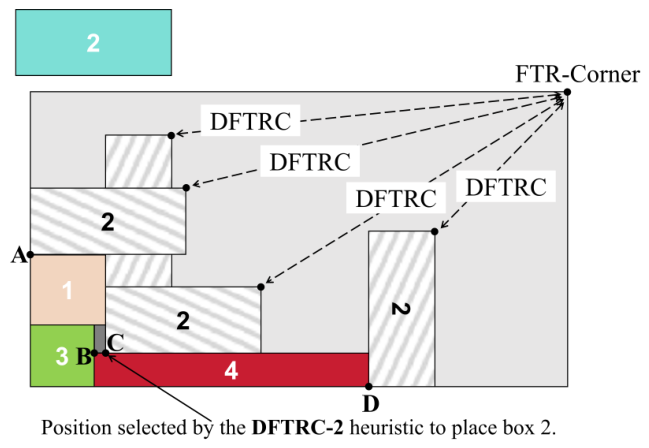
When determining where to place each box, we exclusively evaluate candidate positions located at the origin vertices ( x i ,   y i ,   z i ) of every feasible empty maximal space. We adopt the DFTRC-2 heuristic from [14], which measures compactness by the squared Distance to the Front-Top-Right Corner (DFTRC) of the bin after placement. Higher DFTRC indicates greater compactness. DFTRC-2 evaluates all feasible EMSs and orientations, selecting the one maximizing DFTRC.
An illustrative example is provided in Figure 4. The figure depicts a partial packing configuration containing three already-placed boxes: box 1 (beige), box 3 (green), and box 4 (red). Box 2 (cyan, enlarged in the upper-left corner) is the next item to be packed. Hatched rectangles labeled “2” indicate candidate placements within different EMSs, whose minimum-coordinate corners are marked by black dots A, B, C, and D. The solid arrow demonstrates that DFTRC-2 ultimately selects position C (from EMS corner D) for placing box 2.
The pseudocode of the DFTRC-2 placement heuristic is detailed in Algorithm 3.
Algorithm 3 DFTRC-2 Heuristic Procedure for Box Placement.
Require: Box to pack b, bin b i n
Ensure: Winning EMS E M S and orientation B O , or 0 if not possible
 1:
Let N e m s be the number of available EMSs in bin b i n
 2:
Initialize m a x D i s t 2 1 , B O 1 , E M S 0
 3:
for  i = 1 to N e m s  do
 4:
    Let x , y , z be the min coordinates of E M S i
 5:
    for all possible orientations B O of b do
 6:
        Let d B O , w B O , h B O be the dimensions of b in orientation B O
 7:
        if b fits in E M S i of bin b i n using B O  then
 8:
            D i s t 2 ( D x d B O ) 2 + ( W y w B O ) 2 + ( H z h B O ) 2
 9:
           if  D i s t 2 > m a x D i s t 2  then
10:
                m a x D i s t 2 D i s t 2
11:
                B O B O
12:
                E M S E M S i
13:
           end if
14:
        end if
15:
    end for
16:
end for
17:
return  E M S             ▹ returns 0 if b cannot be packed in b i n

4.3.3. Box Orientation

The orientation of each box is determined by the VBO vector generated by HAGWO. Let EMS denote the empty maximal space chosen by DFTRC-2 for accommodating box i, and let BOs represent the vector containing all admissible orientations of box i within EMS. The selected orientation, B O , is then computed as
B O = B O s ( V B O i × n B O s )
where n B O s indicates the total number of orientations stored in BOs, and x denotes the ceiling of x (i.e., the least integer greater than x).

4.3.4. Placement Procedure

The packing process operates sequentially, with exactly one box being assigned to a bin at each step. The packing sequence of boxes is determined by the BPS generated through HAGWO evolution. This procedure integrates four components: the BPS and VBO vectors produced by HAGWO, the list S b recording all empty maximal spaces for each active bin b, and the DFTRC-2 placement heuristic. Every step of the process consists of five principal substeps:
(1)
Box selection;
(2)
Bin and empty maximal space selection;
(3)
Box orientation selection;
(4)
Box packing;
(5)
State information update.
The pseudocode of the placement procedure is presented in Algorithm 4.
Algorithm 4 Placement Procedure for 3D Bin Packing.
Require: Box packing sequence B P S = [ b 1 , , b n ] , orientation bias vector V B O [ 0 , 1 ] n , initial empty bin template
Ensure: Final set of packed bins B with updated EMS lists
 1:
Initialize B { 1 } , N B 1
 2:
for  i = 1 to n do
 3:
     b B P S i
 4:
     e m s 0 , b i n 0
 5:
    for  k = 1 to N B  do
 6:
         e m s DFTRC - 2 ( b , k , B O )
 7:
        if  e m s > 0  then
 8:
            b i n k
 9:
           break
10:
        end if
11:
    end for
12:
    if  b i n = 0  then
13:
         b i n N B + 1
14:
         B B { b i n }
15:
         N B N B + 1
16:
         e m s 1
17:
    end if
18:
    Let B O s be the feasible orientations of b in e m s of bin b i n
19:
    Let n B O | B O s |
20:
     B O B O s V B O b × n B O
21:
    Pack b at origin of e m s in bin b i n using B O
22:
    Update EMS list of bin b i n via DP procedure [30]
23:
end for

4.3.5. Fitness Function

An evolutionary algorithm necessitates a criterion for evaluating solution quality. For bin packing problems, the total number of bins utilized, denoted as NB, serves as an intuitive quality indicator. Nevertheless, because multiple solutions may yield identical NB values, this metric lacks sufficient discriminatory power when comparing solutions with equivalent bin counts.
To address this limitation, we introduce an enhanced quality measure termed the adjusted number of bins (aNB). This metric integrates NB with an auxiliary indicator—ranging from 0 to 1—that quantifies the improvement potential inherent in a given packing configuration. The underlying principle is as follows: given two solutions with equal NB, the one containing the most underutilized bin offers greater scope for optimization, since the residual capacity in that bin could potentially absorb items currently assigned to other bins, ultimately facilitating a decrease in the overall bin consumption. While a least-loaded bin may sometimes reflect poor utilization, in the context of the aNB fitness function it serves as an indicator of improvement potential rather than a direct measure of packing quality. By combining NB with the normalized least-load ratio, aNB provides a finer gradient for the optimizer to discriminate among solutions with identical bin counts.
We define LeastLoad as the total weight (or volume) contained in the least-loaded bin of a packing configuration. For the 3D variant, the capacity of every bin is given by BinCap = W × H × D . The adjusted number of bins is subsequently obtained by augmenting NB with the ratio of LeastLoad to BinCap:
a N B = N B + L e a s t L o a d B i n C a p .
This fitness encourages both minimizing NB and improving space utilization within bins. The fractional term LeastLoad/BinCap provides differentiation granularity below the integer bin count, guiding the search toward configurations where spare capacity is concentrated in the least-loaded bin, thereby increasing the likelihood of future bin reduction through box rearrangement.

4.4. HAGWO for 3D-BPP

We adapt the HAGWO framework to 3D-BPP, using the same individual representation and decoding procedure described above. Each individual is a real-valued vector of length 2 n [ 0 , 1 ] , divided into two semantic groups of size n (packing sequence and orientation bias). The complete pseudocode is given in Algorithm 5.
The hierarchical adversarial-like mechanism and Levy flight disturbance give HAGWO a greater ability to escape local optima than BRKGA. All other components (maximal spaces, DFTRC-2 placement, aNB fitness) are identical to the BRKGA implementation for fair comparison.
Algorithm 5 HAGWO for 3D-BPP.
Require: Number of boxes n, bin dimensions, box data, population size N, max iterations T max
Ensure: Best fitness, best packing
 1:
Generate initial population X ( N × 2 n ) uniformly in [ 0 , 1 ]
 2:
Evaluate each individual using evaluate (BPS + VBO → placement → aNB)
 3:
Set B e s t P best individual, B e s t V a l u e its aNB
 4:
for  t = 1 to T max  do
 5:
    Sort population by fitness to identify α , β , δ
 6:
    Compute a = 2 2 × ( t / T max )
 7:
    Compute p = 1 t / T max
 8:
    Compute d f = 0.1 × p × Levy ( λ )
 9:
    Determine dynamic group sizes: superior ( n ς ), medium ( n ζ ), inferior ( n ξ )
10:
    for each wolf in superior group do
11:
        Update position using elite averaging and internal exchange (Equation (11))
12:
    end for
13:
    for each wolf in medium group do
14:
        Update position using superior guidance with adversarial-like Levy disturbance (Equation (12))
15:
    end for
16:
    for each wolf in inferior group do
17:
        Update position using medium adversarial-like learning with Levy flight (Equation (13))
18:
    end for
19:
    Apply boundary handling
20:
    Evaluate new positions; apply greedy selection
21:
    Update α , β , δ and B e s t P if improved
22:
    Record best fitness of generation
23:
end for
24:
Return B e s t V a l u e , packing of B e s t P

4.4.1. Distinguishing Optimizer from Decoder Contributions

We acknowledge that all algorithms compared on 3D-BPP—including HAGWO, GWO, PSO, WOA, BSA, CCO, EAO, and BRKGA—share the same encoding–decoding framework (biased random-key encoding, DFTRC-2 placement heuristic, maximal-space management, and aNB fitness function). Therefore, performance differences among these algorithms must be attributed to the optimizer’s ability to navigate the continuous search space  [ 0 , 1 ] 2 n , rather than to the decoding or placement components. The encoding–decoding framework serves as a common “sandbox” in which the metaheuristics compete to discover high-quality packing sequences and orientation biases. HAGWO’s competitive performance in this shared framework demonstrates that its hierarchical adversarial-like search mechanism is effective at finding better solutions within the same representational space, not that the framework itself provides an unfair advantage.

4.4.2. Parallel Implementation

The fitness evaluation phase, which includes random-key decoding, sequential DFTRC-2 placement, and aNB computation, accounts for the majority of the computational cost in the proposed HAGWO algorithm. To accelerate this bottleneck, we employ MATLAB R2020a’s parfor construct for shared-memory parallelization on multi-core CPUs. In each generation, the evaluation of the entire population is distributed across available cores using three separate parfor loops—one for each hierarchical subgroup (superior, medium, and inferior wolves). The dynamic hierarchy assignment, position updates, and greedy selection steps remain sequential due to their low overhead and data dependencies. This parallel strategy achieves near-linear speedup with increasing core count while maintaining the exact algorithmic behavior of the serial version.

5. Experimental Evaluation

This section presents a comprehensive experimental evaluation of the proposed HAGWO. We first validate its performance on the continuous CEC 2017 benchmark suite, followed by its adaptation and evaluation on the three-dimensional single-bin-size bin packing problem (3D-SBSBPP) as a representative real-world combinatorial application. In addition, a component-level ablation study is conducted to quantify the individual contribution of each proposed mechanism (Section 5.5).

5.1. Benchmark Problems and Evaluation Metrics

The bound-constrained single-objective real-parameter optimization test suite from IEEE CEC 2017 [1] is adopted as the principal continuous benchmark. This suite encompasses 30 functions classified into four groups: unimodal (F1–F3), simple multimodal (F4–F10), hybrid (F11–F20), and composition (F21–F30). Function F2 is omitted owing to numerical instability in high-dimensional settings. All functions are assessed at dimensions D = 30 , 50, and 100, with decision space [ 100 , 100 ] D and theoretical minima f min spanning the interval [ 100 , 3000 ] .
The main evaluation criteria are the average (Mean) and standard deviation (Std) of the optimal fitness values obtained across 30 independent executions. Significance testing is conducted via the Wilcoxon signed-rank test at significance level α = 0.05 (the symbols +, ≈, and − denote that HAGWO is significantly superior, statistically equivalent, or significantly inferior to the competitor, respectively) and the Friedman test with mean rank comparison (a lower rank indicates better performance). Furthermore, to ensure the comprehensiveness of statistical validation, we note that the Wilcoxon signed-rank test serves as a distribution-free counterpart to the paired t-test and is suitable for median comparisons without requiring normality assumptions [20]. The Friedman test functions as a rank-based alternative to one-way ANOVA for ranking multiple algorithms across multiple benchmark functions. Collectively, these two tests furnish robust empirical evidence regarding performance differences.

5.2. Parameter Settings and Compared Algorithms

To ensure fairness, all algorithms use the same population size N = 30 and maximum number of iterations T max = 500 . All methods are implemented in MATLAB R2020a and executed on identical hardware (Intel Core i9-9900K @ 3.60 GHz, 32 GB RAM).
The compared algorithms are categorized as follows:
  • Baseline and direct precursor:
    (1)
    Grey Wolf Optimizer (GWO) [10]—the original algorithm from which HAGWO is directly derived.
  • State-of-the-art for 3D Bin Packing:
    (2)
    Biased Random-Key Genetic Algorithm (BRKGA) [14]—a well-established SOTA method for combinatorial packing problems.
  • Classical foundational baselines:
    (3)
    Particle Swarm Optimizer (PSO) [3]—the canonical swarm intelligence paradigm.
  • Other high-performance metaheuristics:
    (4)
    Cuckoo Catfish Optimizer (CCO) [18].
    (5)
    Enzyme Action Optimizer (EAO) [19].
    (6)
    Whale Optimization Algorithm (WOA) [6].
    (7)
    Backtracking Search Algorithm (BSA) [31].
Justification of comparison selection. We acknowledge that several recent GWO variants, such as I-GWO [11], EBGWO [15], IAGWO [9], and SFGWO [16], have demonstrated strong performance on various benchmark suites. These algorithms were not included in our primary comparison for two reasons. First, our comparison set was designed to span diverse algorithmic paradigms (PSO, WOA, BSA, BRKGA, CCO, EAO) to demonstrate HAGWO’s competitiveness against a broad cross-section of metaheuristic approaches, not merely against GWO derivatives. Second, many of these recent GWO variants were published after our initial experiments were completed, or their source code was not publicly available at the time of our study. We consider a comprehensive comparison with all recent GWO variants as valuable future work. All algorithms adopt their original/default parameter settings as recommended in their respective publications. The key parameters are summarized in Table 1.

5.3. Results on Continuous CEC 2017 Benchmark

5.3.1. Qualitative Analysis

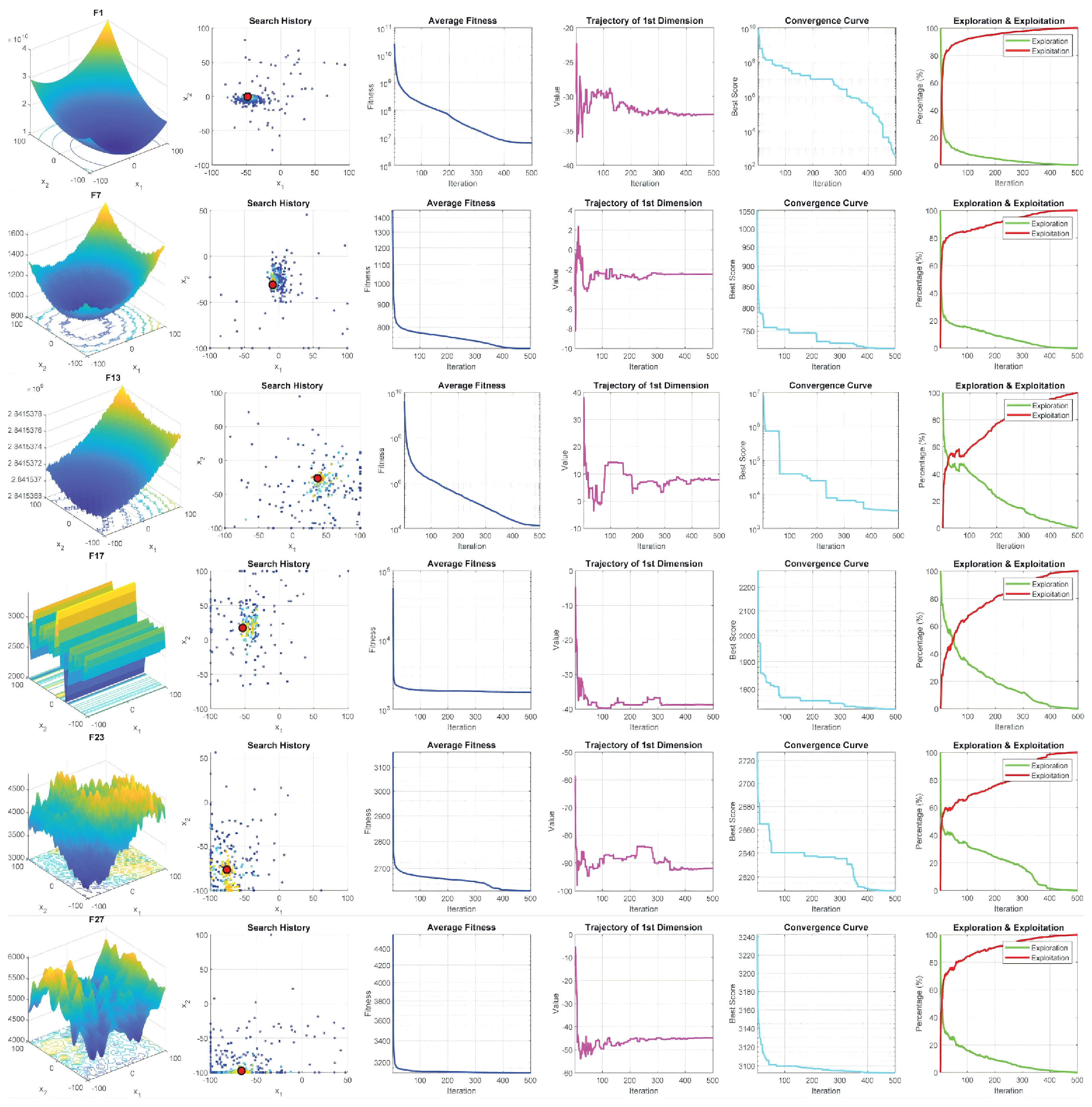
This section qualitatively examines how the proposed HAGWO explores the search space, using six representative 30-dimensional CEC 2017 benchmark functions: the unimodal F1, the simple multimodal F7, the hybrid functions F13 and F17, and the composition functions F23 and F27. The graphical representations include the 3D landscape, historical search traces, mean fitness evolution, trajectory along the first dimension, convergence behavior, and the interplay between exploration and exploitation, as depicted in Figure 5.
The first column displays the 3D surface plots of the selected functions. F1 exhibits a smooth unimodal bowl-shaped landscape with a single global optimum at the origin. In contrast, F7, F13, F17, F23, and F27 present highly complex, rugged, and deceptive landscapes featuring numerous local optima, plateaus, sharp ridges, and variable interactions, posing substantial challenges to optimization algorithms.
As illustrated in the second column (Search History), HAGWO agents initially distribute widely across the search space and progressively converge toward the global optimum (highlighted in red). This convergence pattern is consistently observed across all six functions, with final solutions densely clustered near the optimal area, even on the most deceptive composition functions (F23 and F27).
The average fitness curves (third column) show a sharp decline in the early iterations followed by steady improvement, indicating rapid population enhancement and sustained optimization progress across all function types.
The trajectory of the first dimension (fourth column) exhibits significant fluctuations during the initial phase, reflecting strong global exploration driven by the adversarial-like and Levy mechanisms, followed by rapid stabilization near the optimal value in later iterations. This behavior is particularly evident on hybrid and composition functions (F13, F17, F23, F27), where the trajectory shows multiple large jumps before converging.
The convergence curves (fifth column) reveal fast and stable reduction in the best fitness value with minimal stagnation, even on the most complex composition functions (F23 and F27). HAGWO consistently reaches very low fitness levels efficiently and maintains stability throughout the optimization process.
Finally, the exploration and exploitation trends (sixth column) demonstrate a smooth and effective balance: high exploration rates in the early stage (driven by inferior wolf dominance and Levy flights) gradually give way to increasing exploitation as iterations progress (superior wolf dominance). This dynamic transition enables HAGWO to thoroughly explore the search space while ensuring accurate convergence to high-quality solutions.
Overall, these qualitative visualizations confirm that HAGWO achieves an excellent exploration–exploitation trade-off, contributing significantly to its robust performance across functions of varying complexity and modality.

5.3.2. Quantitative Analysis

This section presents a comprehensive performance comparison of the proposed HAGWO against seven representative metaheuristic algorithms—BSA, BRKGA, GWO, PSO, WOA, EAO, and CCO—on the twenty-nine 30-dimensional CEC2017 benchmark functions (excluding F2). The detailed statistical results, including mean fitness values, standard deviations, Wilcoxon rank-sum test p-values (with HAGWO as the reference), and Friedman rankings, are summarized in Table A1, where the best mean value for each function is highlighted in bold. The following observations are drawn from these results.
  • On the unimodal functions F1 and F3, HAGWO ranks third on F1 (behind CCO and BSA) and third on F3 (behind GWO and CCO). Although not the absolute best, HAGWO maintains competitive mean values and relatively low standard deviations, indicating solid exploitation capability on unimodal landscapes.
  • For the simple multimodal functions F4–F10, HAGWO consistently achieves the best mean fitness on F4, F5, F6, F7, F8, F9, and F10. It demonstrates the lowest (or highly competitive) mean values and low standard deviations across this group, highlighting stable and effective search performance on functions with a moderate number of local optima.
  • On the hybrid functions F11–F20, HAGWO records the best mean fitness on F16, F17, and F20, and ranks second on F11. It remains competitive on most others (e.g., third on F12, F18; fourth on F13, F19). While BSA outperforms on several instances (F12, F14, F15, F18, F19), HAGWO exhibits strong overall robustness in handling complex landscapes with variable interactions and multiple optima.
  • For the composition functions F21–F30, which are the most challenging, HAGWO secures the best mean fitness on F21, F23, F24, F25, F26, F27, F28, and F29. It ranks first or is highly competitive on most instances, with particularly strong performance on F27–F29 (lowest means and competitive standard deviations). These results confirm HAGWO’s superior ability to balance exploration and exploitation in highly composite and deceptive landscapes.
  • The +/≈/− summary row in Table A1 reports the outcomes of the Wilcoxon rank-sum test at a significance level of α = 0.05 (with HAGWO as the reference). HAGWO significantly outperforms BSA on 22 functions (1 tie), BRKGA on 24 functions (1 tie), GWO on 21 functions (3 ties), PSO on all 29 functions, WOA on 25 functions (1 tie), EAO on all 29 functions, and CCO on 20 functions (4 ties).
    The last two rows tabulate the Friedman mean rankings aggregated over the 29 test functions for the eight competing algorithms. HAGWO registers the lowest average rank of 2.07, thus occupying the foremost position, with BSA (3.14), GWO (3.31), CCO (3.93), WOA (4.86), BRKGA (4.90), EAO (6.83), and PSO (6.97) trailing behind.
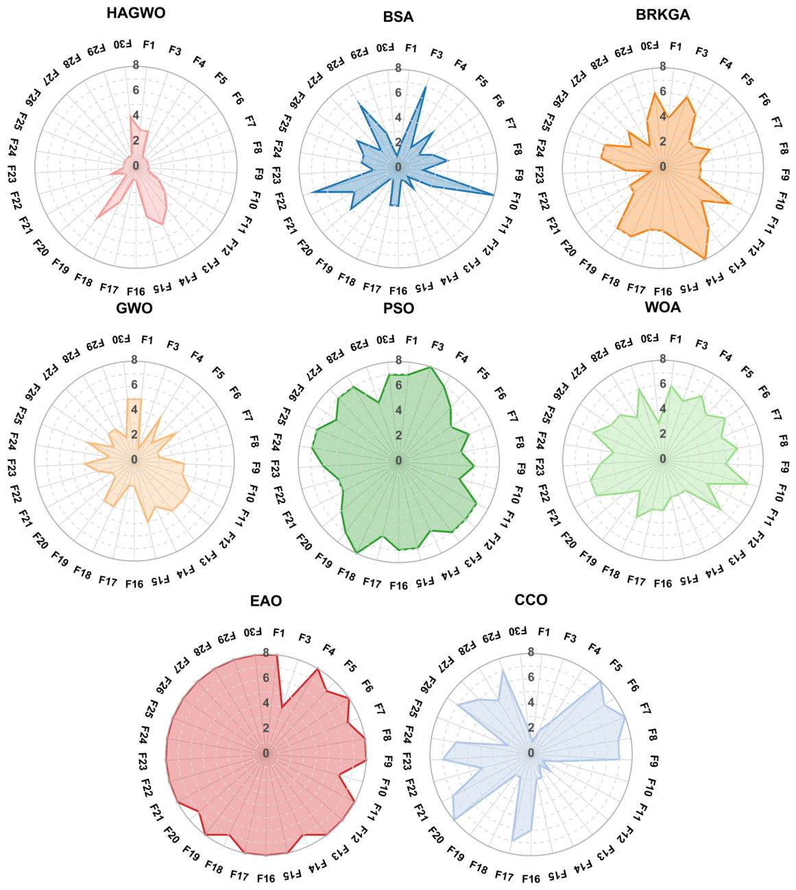
    These findings, corroborated by both the Wilcoxon rank-sum test and the Friedman ranking analysis, compellingly attest to HAGWO’s dominant overall performance and strong robustness across the CEC2017 benchmark suite. The radar ranking plots comparing HAGWO with the seven rival algorithms (Figure 6) offer additional confirmation: the markedly reduced shaded area of HAGWO signals its remarkable stability and comprehensive optimization prowess over diverse functional topologies.

5.4. Convergence Analysis

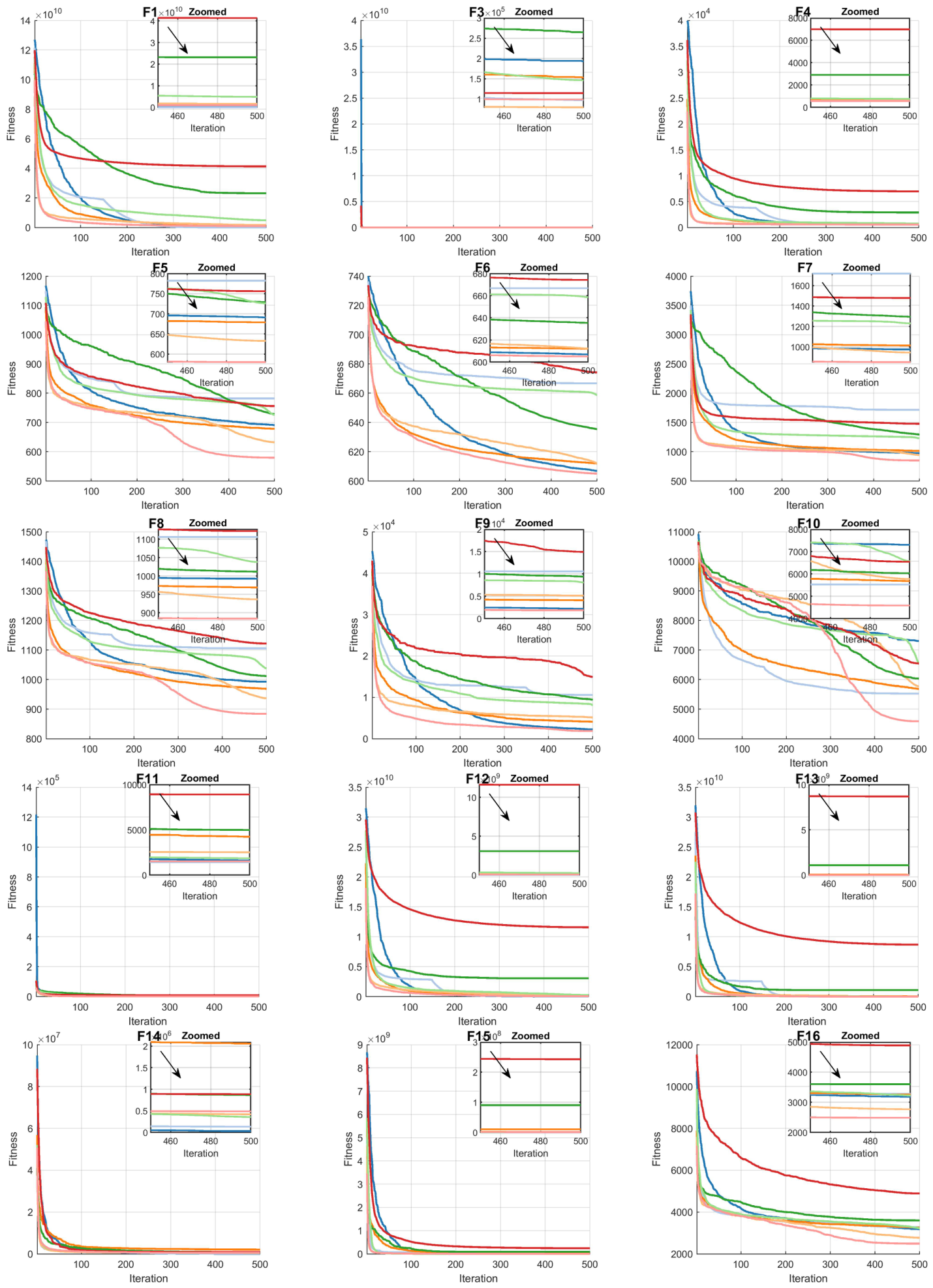
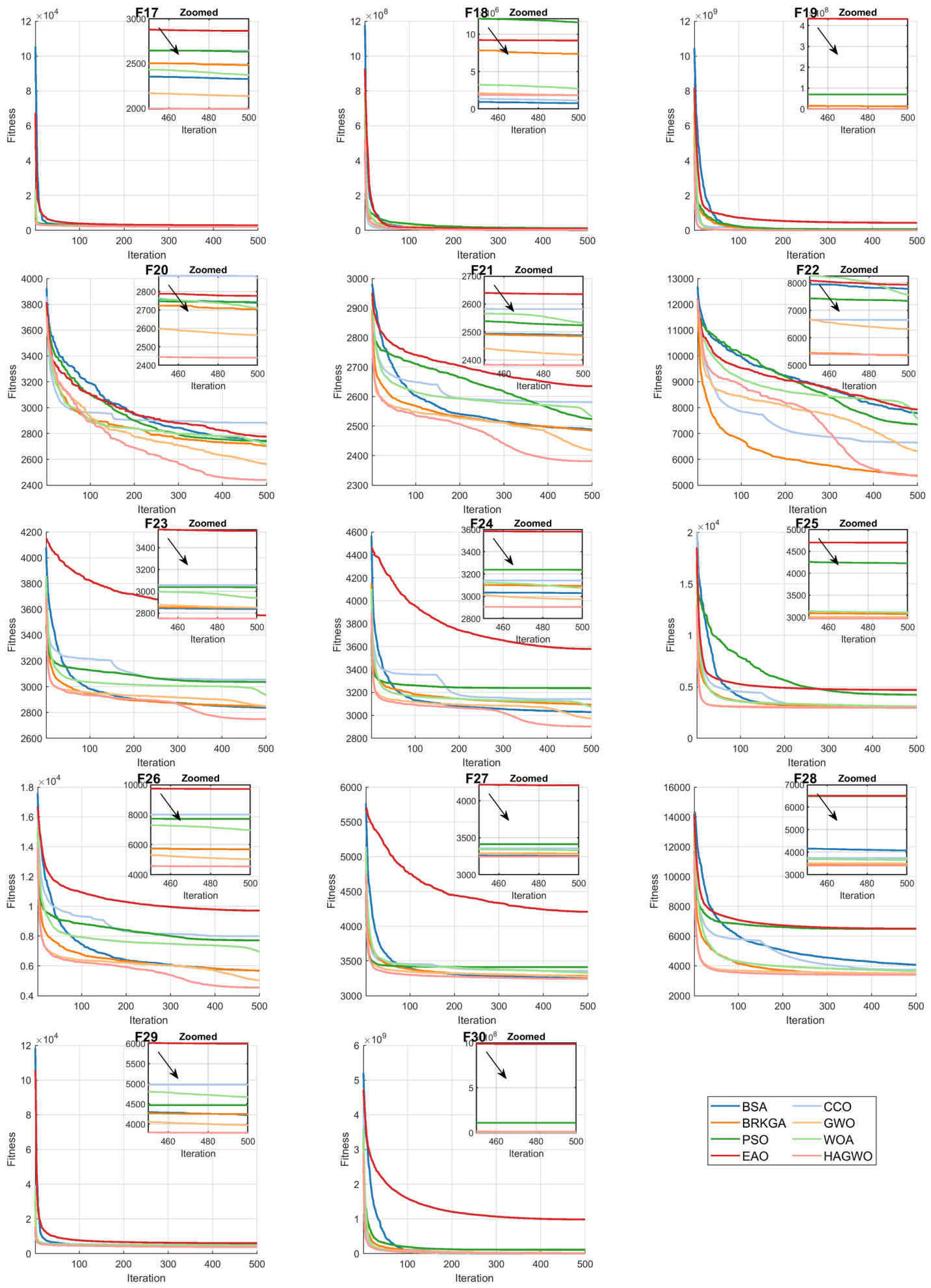
The convergence curves of the proposed HAGWO alongside comparative algorithms (BSA, BRKGA, GWO, PSO, WOA, EAO, and CCO) on the 30-dimensional CEC2017 benchmark suite (excluding F2) are illustrated in Figure A1 and Figure A2, covering unimodal, multimodal, hybrid, and composition functions.
For unimodal functions, HAGWO demonstrates remarkable convergence precision on F1, F3, and F4. On F1, its curve descends steeply toward near-zero fitness values within the first 50 iterations, substantially outperforming PSO and EAO, which plateau at markedly elevated levels. Similarly, on F3 and F4, HAGWO stabilizes at the lowest fitness band, leaving the original GWO, PSO, and EAO far behind in the zoomed subplots.
Regarding multimodal functions, HAGWO upholds excellent competitiveness in both convergence pace and final accuracy. On F5, F6, F7, F8, and F10, the HAGWO curve settles at the bottom of the zoomed views, consistently achieving lower fitness values than GWO, PSO, WOA, and EAO. Notably, on F9 and F10, HAGWO maintains a decisive lead over EAO and PSO, which exhibit pronounced stagnation in later iterations. Even on challenging multimodal landscapes, HAGWO avoids premature halting and continues steady refinement.
For hybrid functions, HAGWO pinpoints viable regions rapidly and transitions effectively to fine-grained exploitation. On F11 through F15 and F17 through F19, HAGWO converges to near-optimal values swiftly, with its curve lying at or near the lowest position across all competitors. The zoomed subplots for F16 and F17 clearly reveal HAGWO’s advantage over GWO, PSO, and EAO by a noticeable margin. On F20, HAGWO preserves its downward trajectory where several rivals level off prematurely.
Concerning composition functions, HAGWO delivers robust and steady performance amid increased complexity. On F21, F22, F23, F24, F25, F26, F28, F29, and F30, the zoomed insets confirm that HAGWO stabilizes at the lowest fitness levels, outperforming the majority of peers. On F27, HAGWO remains highly competitive, closely matching or marginally surpassing the best-performing lines. In contrast, EAO commonly suffers from early stagnation across this category, and PSO frequently settles at suboptimal plateaus.
Collectively, the convergence profiles demonstrate that HAGWO achieves a favorable balance between exploration and exploitation. It reduces fitness rapidly during the early search phase and sustains effective refinement throughout later iterations. Compared with the original GWO and other state-of-the-art metaheuristics, HAGWO exhibits consistently faster and more stable convergence across the majority of the 30-dimensional CEC2017 test cases, validating its superior optimization capability.

5.4.1. Boxplot Analysis

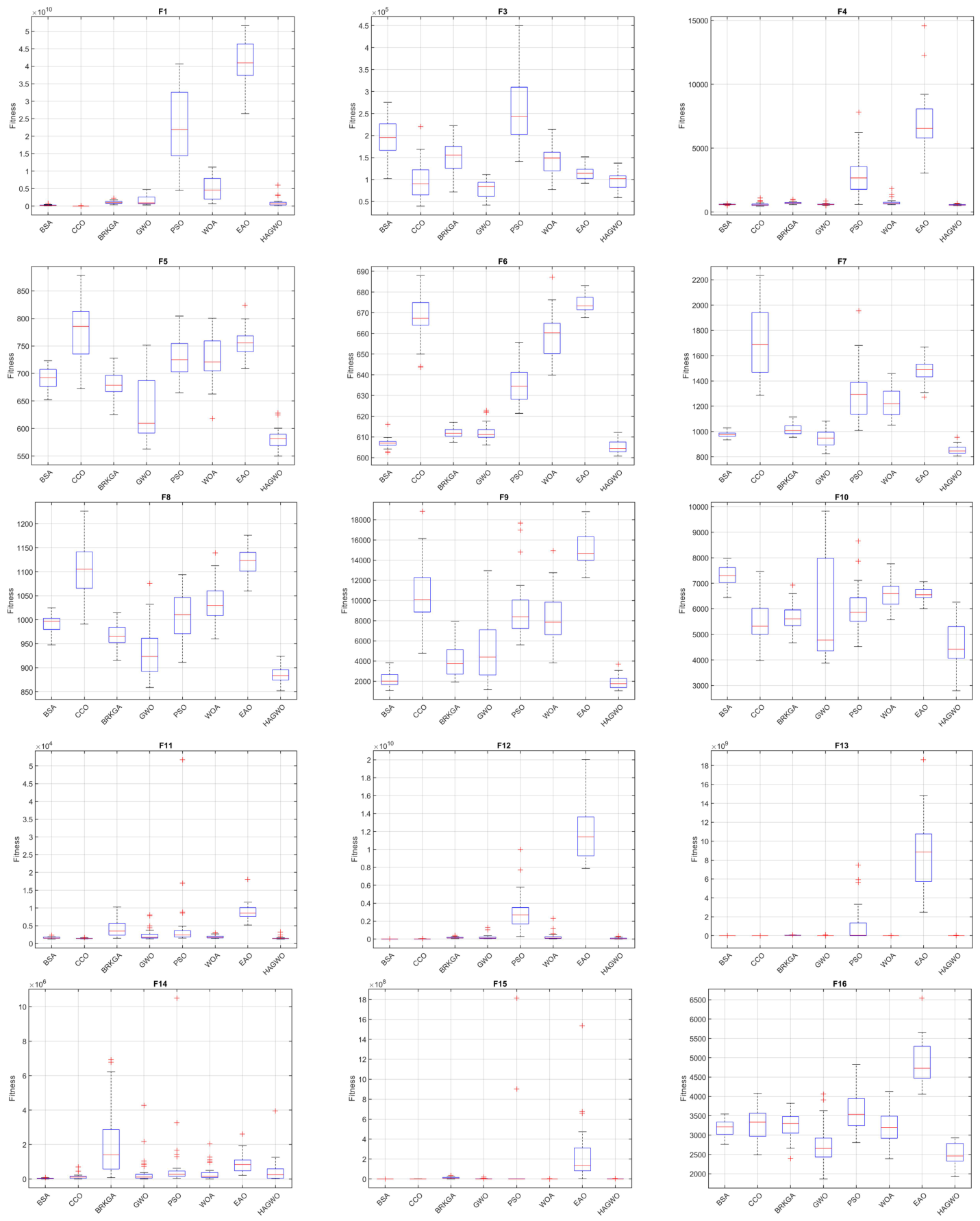
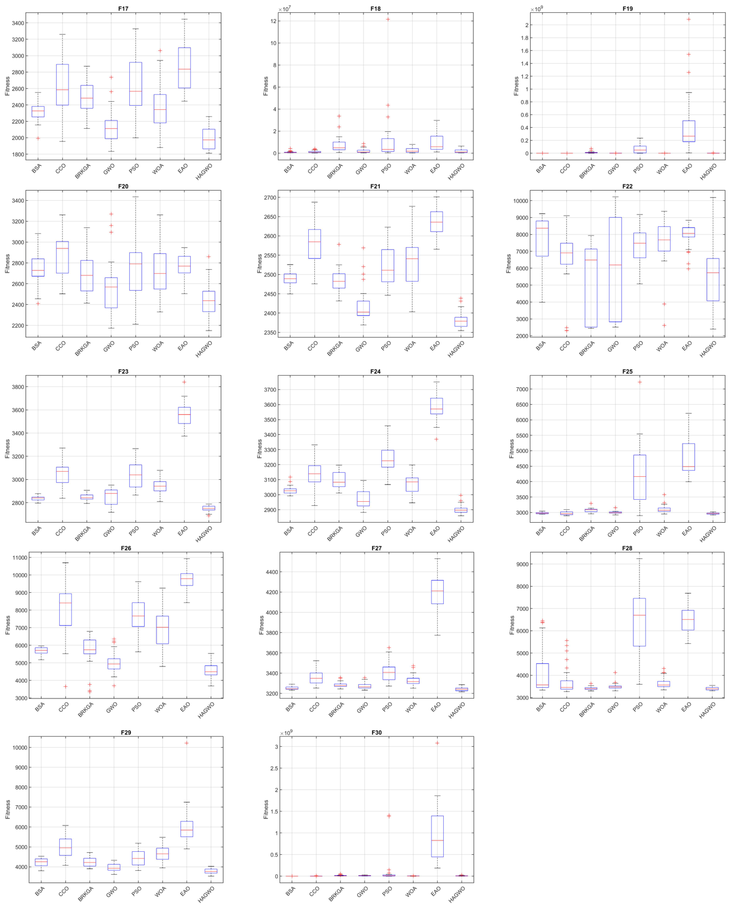
Figure A3 and Figure A4 present the boxplots of the proposed HAGWO and the seven competing algorithms (BSA, BRKGA, GWO, PSO, WOA, EAO, and CCO) on the twenty-nine 30-dimensional CEC2017 benchmark functions (excluding F2) over 30 independent runs. In each boxplot, the central line represents the median, the box indicates the interquartile range (IQR), the whiskers extend to the minimum and maximum values within 1.5 × IQR, and outliers are marked with red plus signs (+). HAGWO corresponds to the rightmost box in each subplot.
The boxplots reveal that HAGWO consistently achieves the lowest median fitness values across almost all 29 functions. Moreover, HAGWO exhibits the smallest IQR (tightest box) and the fewest (or zero) outliers in the vast majority of cases, indicating superior stability and robustness. This advantage is particularly evident on challenging functions such as F1, F3, F5, F6, F7, F8, F9, F11, F12, F13, F15, F16, F18, F19, F21, F23, F24, F25, F26, F27, F28, F29, and F30, where most competing algorithms display large spreads, long whiskers, and numerous outliers, while HAGWO maintains a compact distribution tightly clustered around a low median.
These results demonstrate that HAGWO not only finds better solutions (consistent with the mean values in Table A1) but also delivers highly consistent performance across unimodal, multimodal, hybrid, and composition functions. The narrow boxes and minimal outliers confirm HAGWO’s strong ability to avoid premature convergence and maintain reliable optimization behavior in complex, high-dimensional search landscapes.

5.4.2. Scalability Analysis

Engineering optimization problems in practical settings frequently exhibit high-dimensional characteristics, thereby imposing considerable demands on algorithmic scalability and robustness. To rigorously assess how HAGWO performs as problem complexity escalates, we carried out experiments on 29 benchmark functions drawn from the CEC2017 suite at dimensionalities of 50 and 100, yielding 58 high-dimensional test cases in total. The performance of HAGWO relative to seven competing algorithms is detailed in Table A2 and Table A3.
In the 50-dimensional setting, HAGWO achieves the best mean value on 24 out of 29 functions (82.8%). In the 100-dimensional setting, HAGWO achieves the best mean value on 22 out of 29 functions (75.9%). These results demonstrate that HAGWO maintains strong performance across all tested dimensionalities, with only a moderate decrease in the proportion of best solutions at D = 100, which is expected due to the dramatically increased search space complexity.
The Wilcoxon signed-rank test results (significance level α = 0.05 ) reported in the tables provide statistical evidence of HAGWO’s competitive superiority. For the 50-dimensional functions, HAGWO significantly outperforms BSA on 22 functions (1 tie), BRKGA on 24 functions (1 tie), GWO on 21 functions (3 ties), PSO on all 29 functions, WOA on 25 functions (1 tie), EAO on all 29 functions, and CCO on 20 functions (4 ties). For the 100-dimensional functions, HAGWO significantly outperforms BSA on 27 functions (1 tie), BRKGA on 27 functions (2 ties), GWO on 24 functions (3 ties), PSO on 26 functions (1 tie), WOA on 27 functions (2 ties), EAO on 28 functions (1 tie), and CCO on 23 functions (3 ties). These results indicate that HAGWO maintains statistically significant superiority on the vast majority of benchmark functions across both dimensionalities, with only a slight increase in ties at D = 100 and virtually no losses.
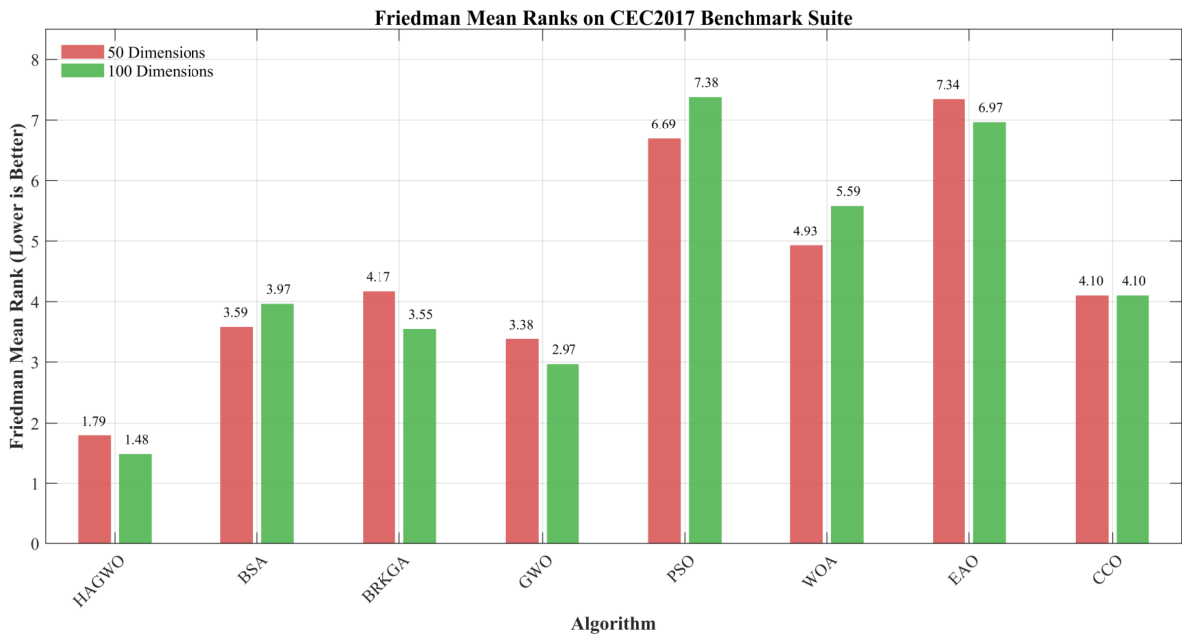
The Friedman mean rank results shown in Figure 7 further support this observation. In the 50-dimensional setting, HAGWO attains the lowest mean rank of 1.83, securing the overall 1st place, followed by CCO, GWO, BSA, BRKGA, WOA, EAO, and PSO. In the 100-dimensional setting, HAGWO attains the lowest mean rank of 1.62, again securing the 1st place, followed by GWO, BRKGA, CCO, WOA, EAO, BSA, and PSO. These consistent top rankings across increasing dimensionalities confirm HAGWO’s excellent scalability and superior overall performance in high-dimensional optimization scenarios.

5.5. Ablation Study

To verify that each of the three proposed mechanisms contributes meaningfully to the overall performance of HAGWO, we conduct a component-level ablation study on the CEC 2017 benchmark suite at 30D. Three ablated variants are constructed by disabling exactly one mechanism while keeping the others intact:
  • HAGWO-w/o-S (without fitness-based hierarchical stratification): the assignment of individuals to the superior, medium, and inferior tiers is randomized instead of being guided by fitness ranking, while the three group-specific update rules, the group proportions, and the dynamic switching schedule are all preserved. This isolates the contribution of fitness-guided stratification itself.
  • HAGWO-w/o-A (without hierarchical adversarial-like updating): the stratification structure is preserved, but all groups adopt the standard GWO position update; the directed and opposition-based perturbations are removed, while the Lévy flight term is retained as an undirected random perturbation with the same decay schedule.
  • HAGWO-w/o-L (without adaptive Lévy flight): the full hierarchical adversarial structure is preserved, but the Lévy perturbation factor is set to zero in all update rules.
The original GWO is additionally included as the baseline in which all three mechanisms are absent. Since this ablation study requires regenerating all control groups from scratch, the full HAGWO and all its variants are re-executed using the same set of random seeds. Consequently, the HAGWO results reported in Table 2 may differ slightly from those in the main experiments (Table A1), as the latter belong to an independent experimental campaign. All variants are evaluated under the same experimental protocol, as outlined in Section 5 (population size 30, 500 iterations, 30 independent runs), on the 29 CEC 2017 functions at 30D. The results, together with Wilcoxon signed-rank tests against the full HAGWO and Friedman mean ranks, are summarized in Table 2.
Three observations can be drawn. First, the original GWO, in which all three mechanisms are absent, ranks last by a wide margin (Friedman mean rank 4.83 versus 1.90–2.97 for all HAGWO-based variants) and is significantly outperformed by the full HAGWO on 22 of the 29 functions. This confirms that the performance gains reported in this section stem from the proposed mechanisms rather than from implementation details.
Second, and most importantly, removing any single mechanism degrades the overall performance: the Friedman mean rank of the full HAGWO (1.90) deteriorates to 2.45, 2.86, and 2.97 when the stratification, the adversarial-like updating, and the Lévy flight are removed, respectively. This monotonic degradation provides direct experimental evidence that each of the three components contributes meaningfully and non-redundantly to the observed performance gains.
Third, the three mechanisms exhibit distinct contribution patterns. (i) For HAGWO-w/o-S, replacing fitness-guided tier assignment with random assignment degrades the mean rank from 1.90 to 2.45; the variant is significantly worse on F4 and never significantly better on any function (28 ties out of 29). This indicates that it is the fitness-guided partitioning—rather than the mere existence of groups—that directs the appropriate update rule to the appropriate individuals at each search stage. (ii) HAGWO-w/o-A exhibits the largest number of significant degradations (9 functions), concentrated on simple multimodal (F5–F8, F10) and composition (F21–F24) landscapes, confirming that the tier-differentiated adversarial-like rules are the primary performance-driving component. The variant surpasses the full model only on four functions (F3, F13, F14, F28), suggesting occasional over-guidance of the directed updates on certain hybrid landscapes, but the net effect of removing this mechanism is clearly negative. (iii) HAGWO-w/o-L attains the worst mean rank (2.97) among all HAGWO variants, with a significant degradation on F24 and consistently elevated mean values across most of the suite, indicating that the adaptive Lévy flight perturbation supports fine-grained exploitation and escape from suboptimal regions, particularly on composition functions where precise convergence is required.
Overall, the ablation results demonstrate that the integrated HAGWO framework yields large and statistically significant gains over the original GWO, and that the hierarchical stratification, the adversarial-like updating, and the Lévy flight perturbation each provide significant and complementary contributions, consistent with the synergistic design rationale discussed in Section 3.3.3.

5.6. Results on 3D Bin Packing Benchmark

To evaluate the performance of the proposed HAGWO on the constrained combinatorial problem of 3D-BPP with identical bins (3D-SBSBPP), we adapt it using biased random-key encoding and the DFTRC-2 placement heuristic. For fair comparison, all algorithms—including the original GWO, BRKGA, WOA, PSO, BSA, CCO, and EAO—were implemented with the same encoding scheme, DFTRC-2 heuristic, maximal-space management, and adjusted fitness function (aNB). In this subsection, we use the original algorithm names for brevity, with the understanding that all results reflect the adapted versions on 3D-SBSBPP.
The comparison is performed on the standard benchmark set by Martello et al. [2], containing 160 instances across 8 classes (20 instances per class: 10 with n = 50 items and 10 with n = 100 ). Classes 1–5 use bin dimensions 100 × 100 × 100 and five item types with the size ranges shown in Table 3, where each item of type k is selected with probability 0.6 and each of the other types with probability 0.1. Classes 6–8 employ different bin sizes and item dimension ranges as follows:
  • Class 6: bin 10 × 10 × 10 ; dimensions [ 1 , 10 ] .
  • Class 7: bin 40 × 40 × 40 ; dimensions [ 1 , 35 ] .
  • Class 8: bin 100 × 100 × 100 ; dimensions [ 1 , 100 ] .
All algorithms use a population size of N = 50 and run for 100 generations. Experiments are conducted on the same hardware (Intel Core i9-9900K @ 3.60 GHz, 32 GB RAM) using MATLAB R2020a. Each algorithm is executed with 10 independent runs using different random seeds (seed = 1 , 2 , , 10 ) to ensure reproducibility.

5.6.1. Quantitative Results

Average results over 10 independent runs are summarized in Table 4. Lower values of aNB (adjusted fitness) and NB (number of bins) indicate better performance; aT reports average runtime in seconds. The “Total” NB is the sum of average NB values across all 160 instances (scaled by 10 runs), with the best result in bold.
The experimental results demonstrate the effectiveness of HAGWO for the 3D-BPP. Overall, GWO achieves the best performance with the lowest total NB of 2944. HAGWO ranks second with a total NB of 2967, outperforming BRKGA (2989) by 22 bins and showing clear gains over PSO (2999), BSA (3009), CCO (3012), and EAO (3041). Similar trends appear in the average fitness (aNB) column.
A closer look at class-specific performance reveals interesting patterns. In the more constrained and difficult classes (1, 2, 3, 6, 7, 8), particularly at n = 100 , HAGWO consistently narrows the gap with GWO and widens its advantage over BRKGA and other methods. For example, in Class 7 ( n = 100 ), HAGWO reduces the average NB by 0.3 bins compared to BRKGA while maintaining comparable runtime. In contrast, on easier classes (4 and 5), almost all algorithms converge to nearly identical NB values, suggesting that the problem instances are less discriminative when near-optimal packings are readily achievable. This behavior aligns with the intrinsic difficulty gradient of the benchmark: classes with higher item-size variability and tighter spatial constraints benefit more from HAGWO’s hierarchical adversarial-like updates and adaptive Levy perturbations, which help escape suboptimal packing sequences.
Moderation of superiority claims. We acknowledge that HAGWO does not dominate all competitors on 3D-BPP; specifically, the original GWO achieves a marginally lower total bin count (2944 vs. 2967). This outcome is consistent with the No Free Lunch theorem [32]: no single algorithm excels universally across all problem landscapes. The original GWO’s simpler, leader-centric hierarchy appears particularly effective under the strict geometric and non-overlapping constraints of 3D-BPP, where precise local adjustments to packing sequences are critical. However, HAGWO’s substantial advantage in run-to-run stability (narrowest IQR and fewest outliers across 13 of 16 instance groups) and its clear superiority over BRKGA, PSO, BSA, CCO, and EAO demonstrate that the proposed hierarchical adversarial-like framework provides meaningful benefits in constrained combinatorial settings, even if it marginally trails the original GWO in raw bin count on this specific benchmark.
In terms of computational efficiency (aT), GWO and HAGWO maintain competitive running times across most classes, especially on larger instances (Classes 4–5 and 8), while still delivering superior packing quality. These results confirm that the hybrid adaptive mechanism in HAGWO provides a robust balance between solution quality and efficiency.

5.6.2. Boxplot Analysis

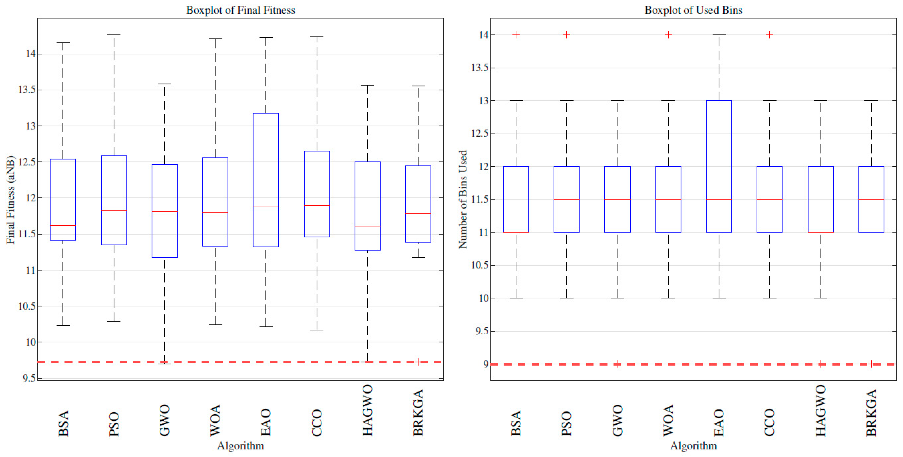
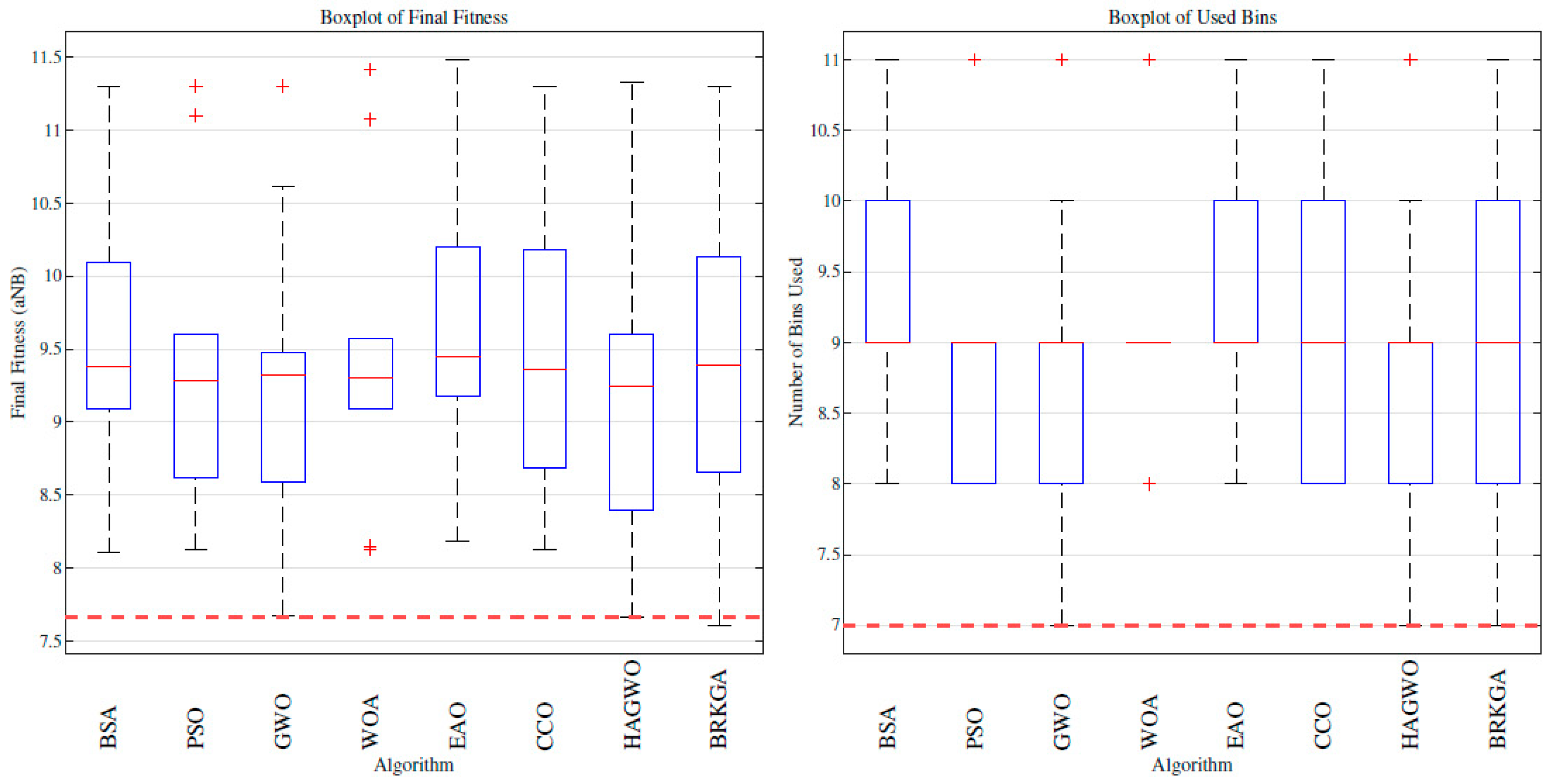
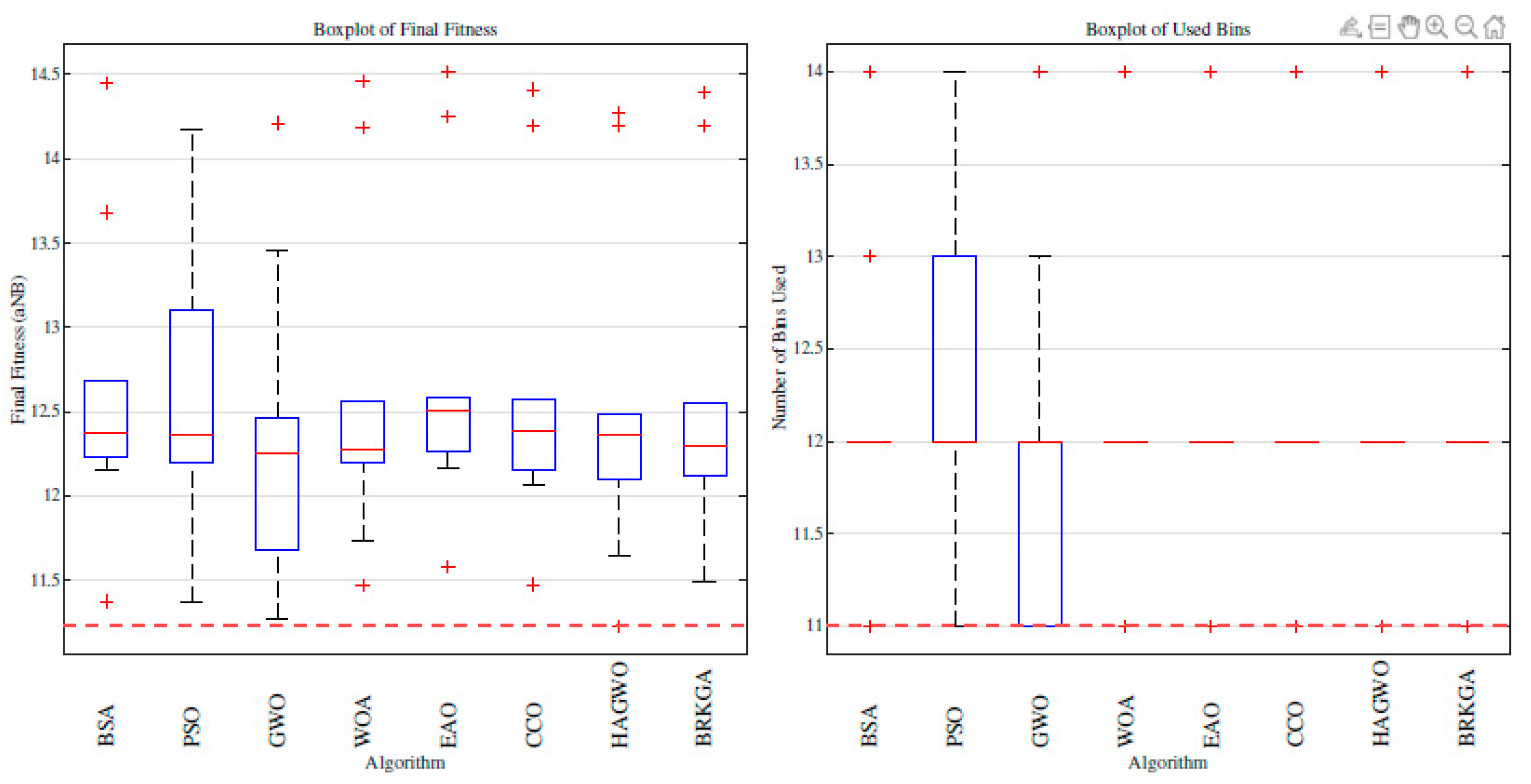
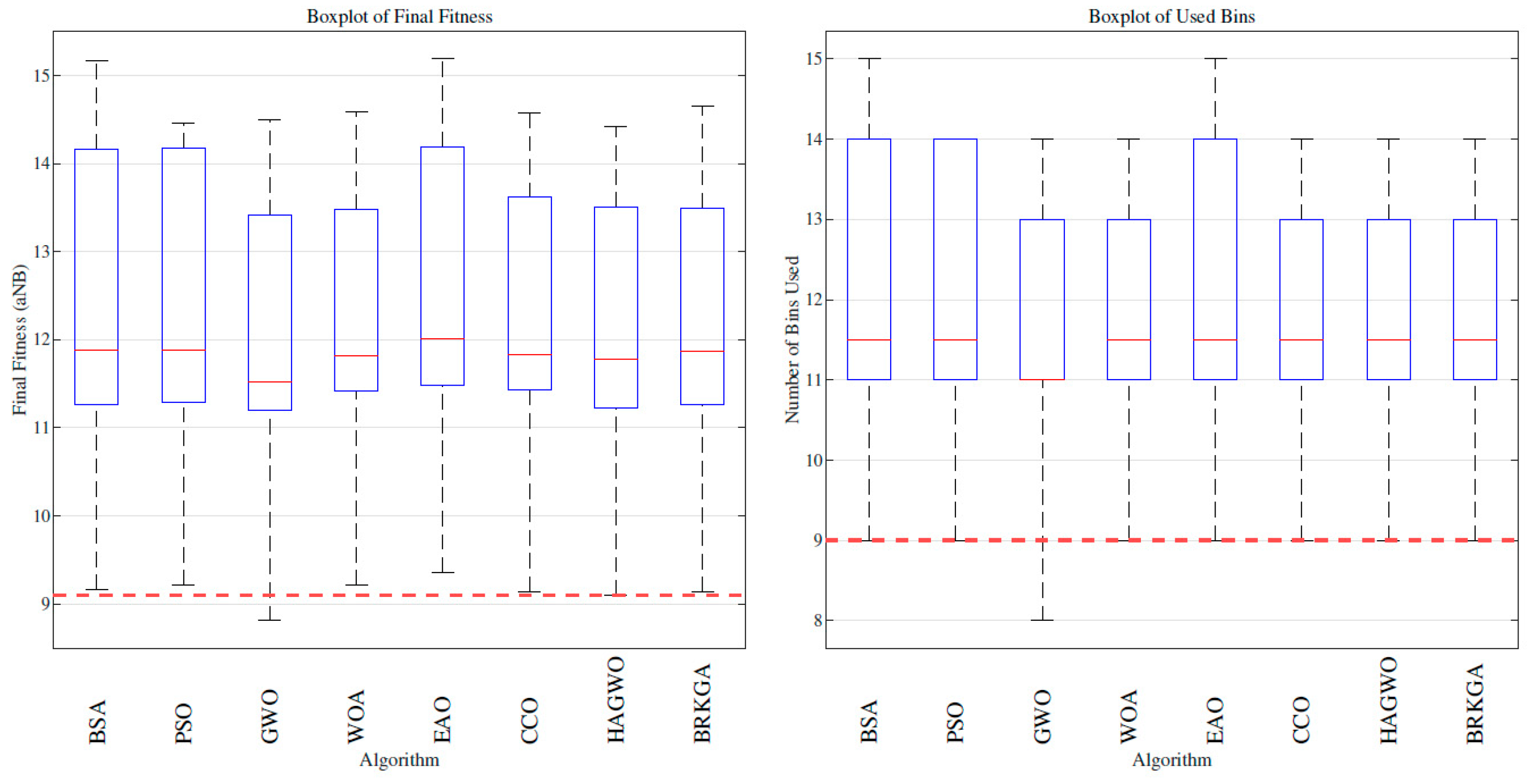
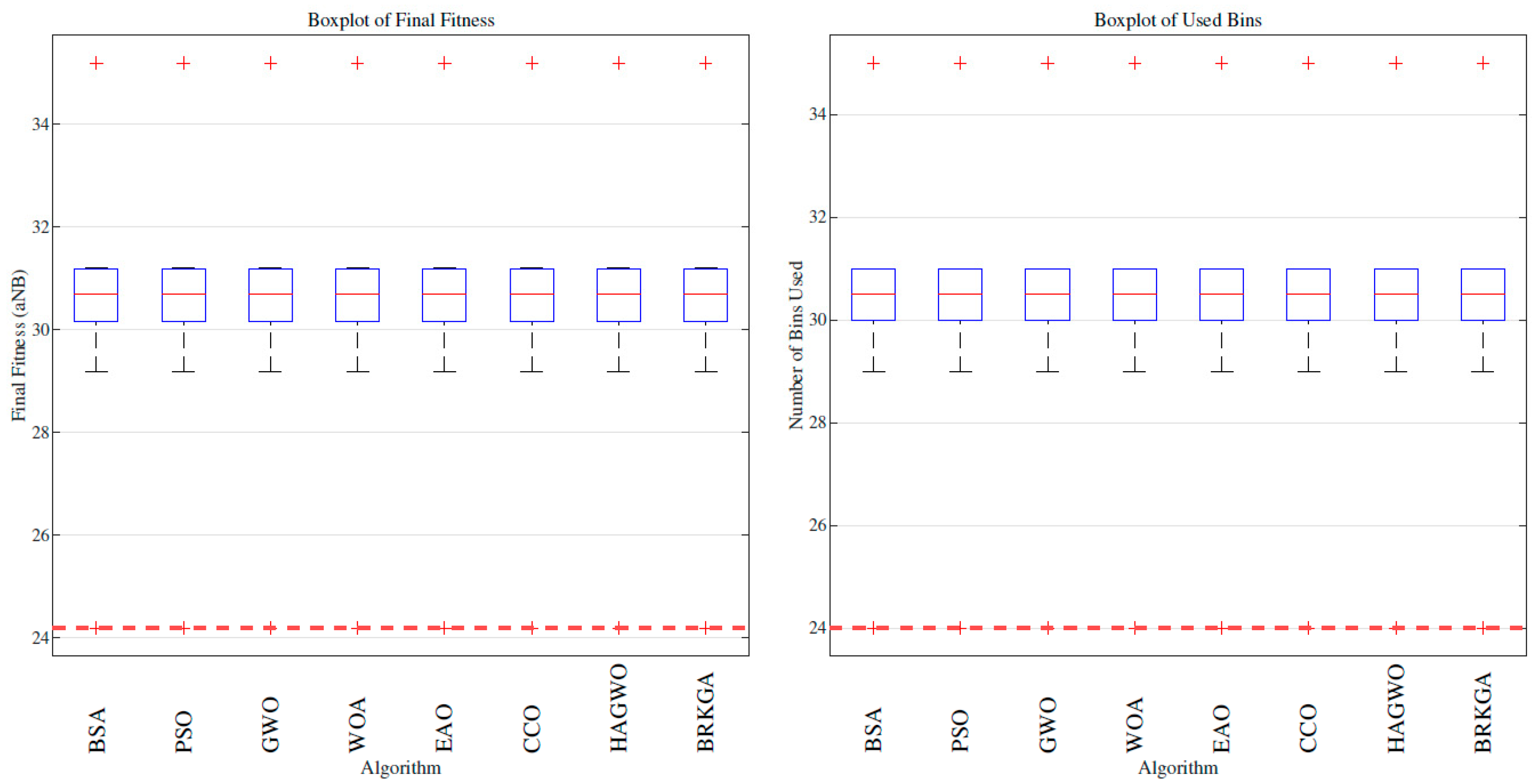
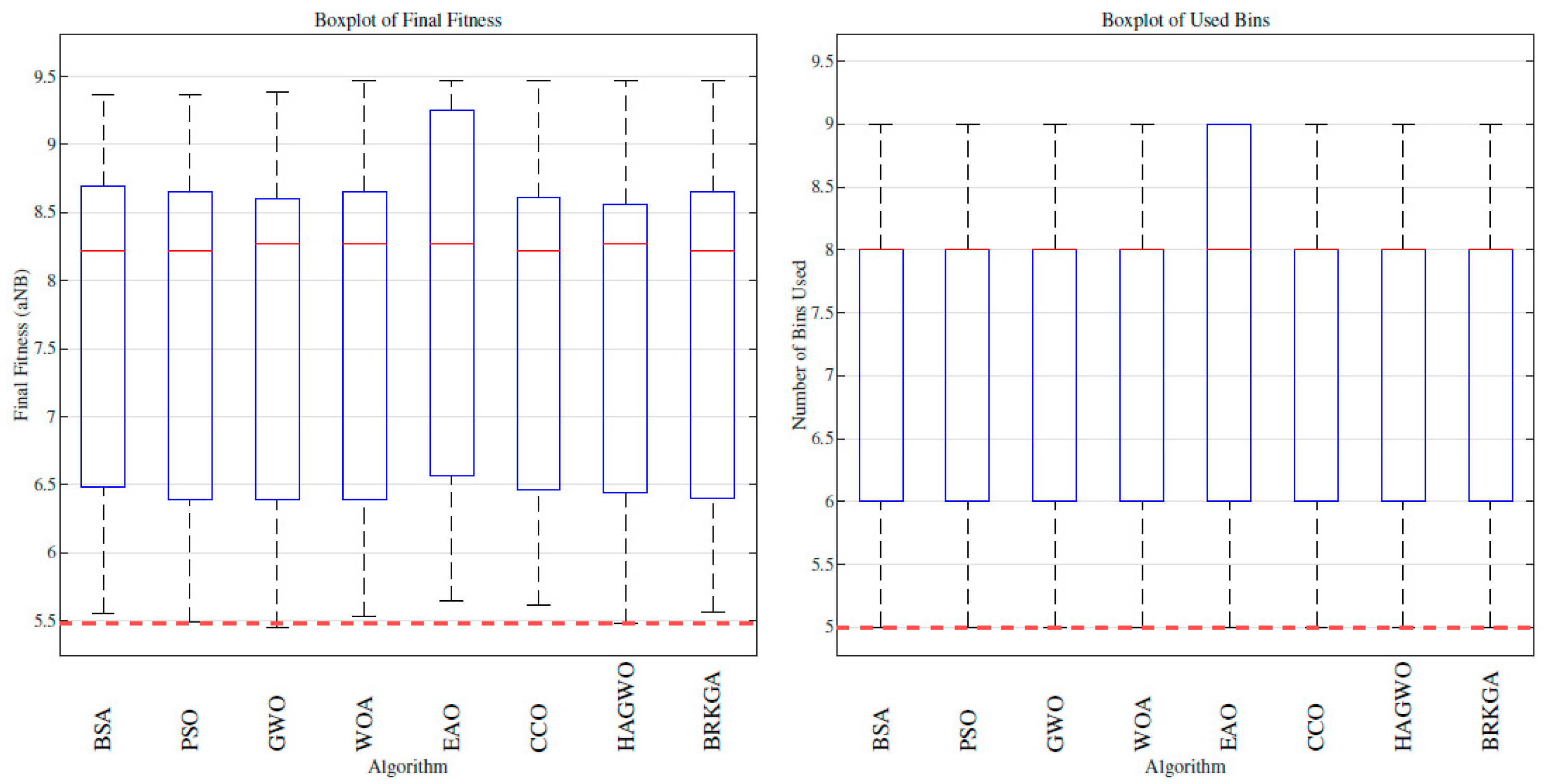
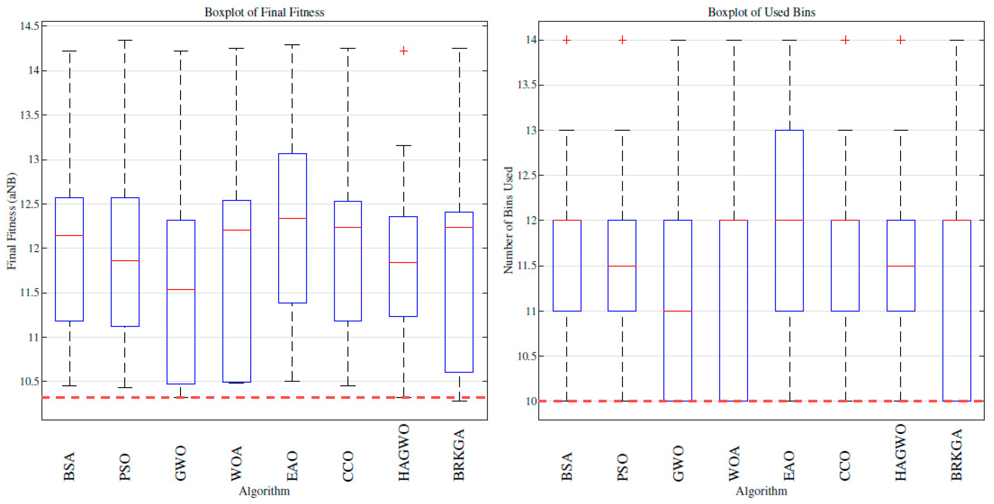
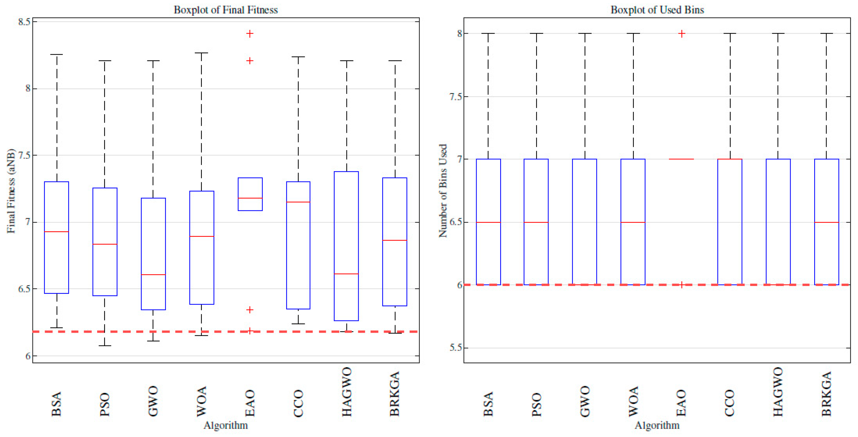
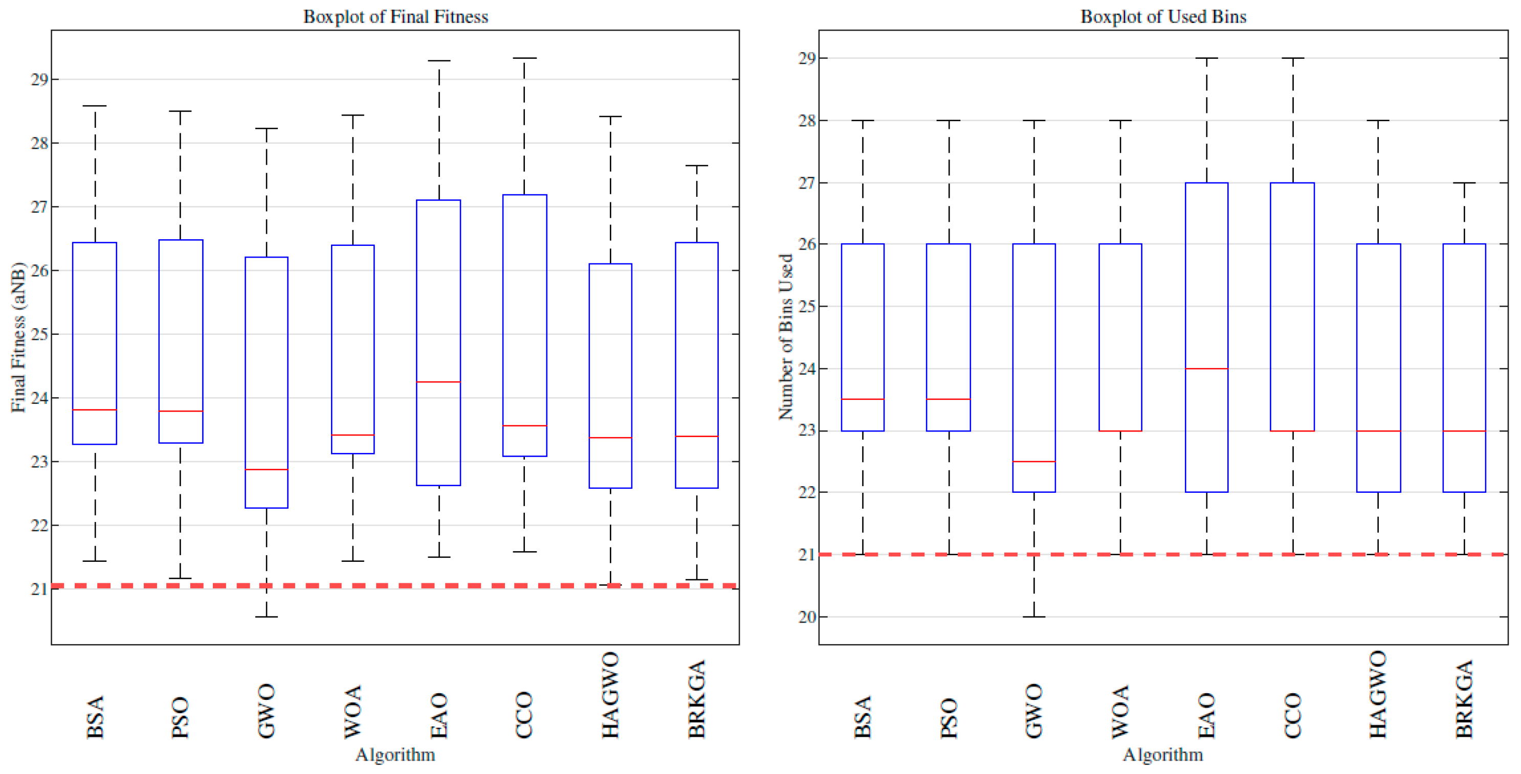
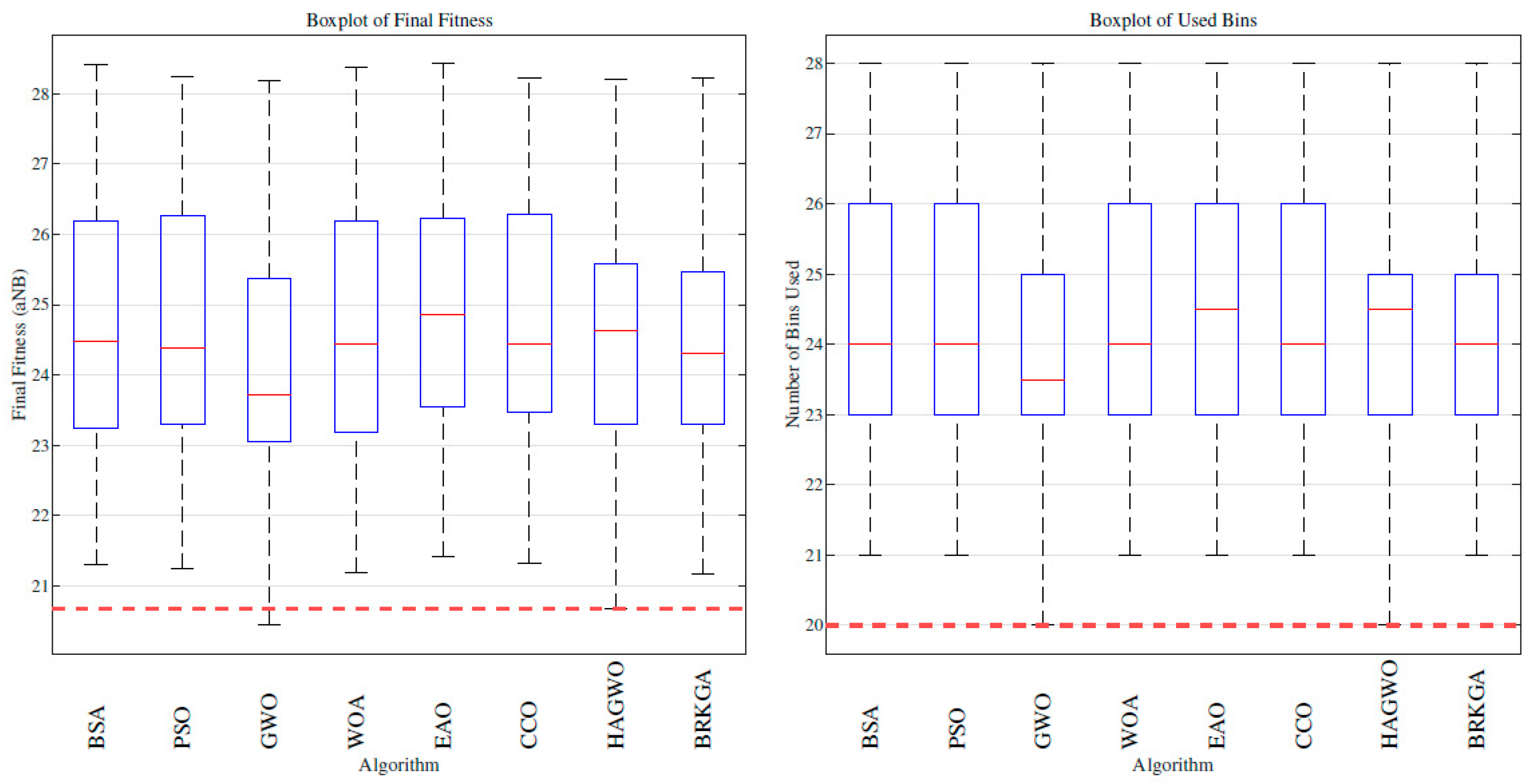
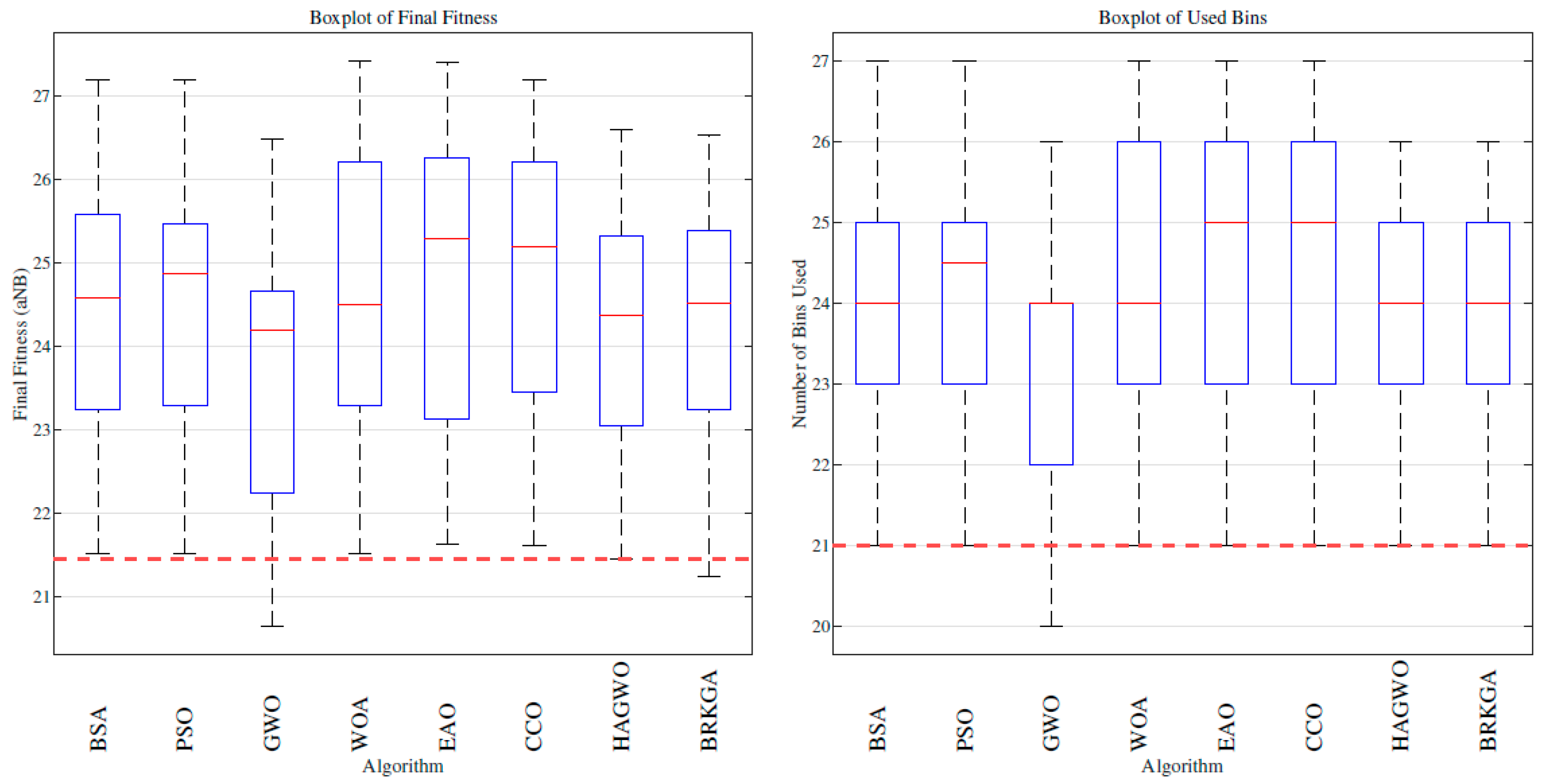
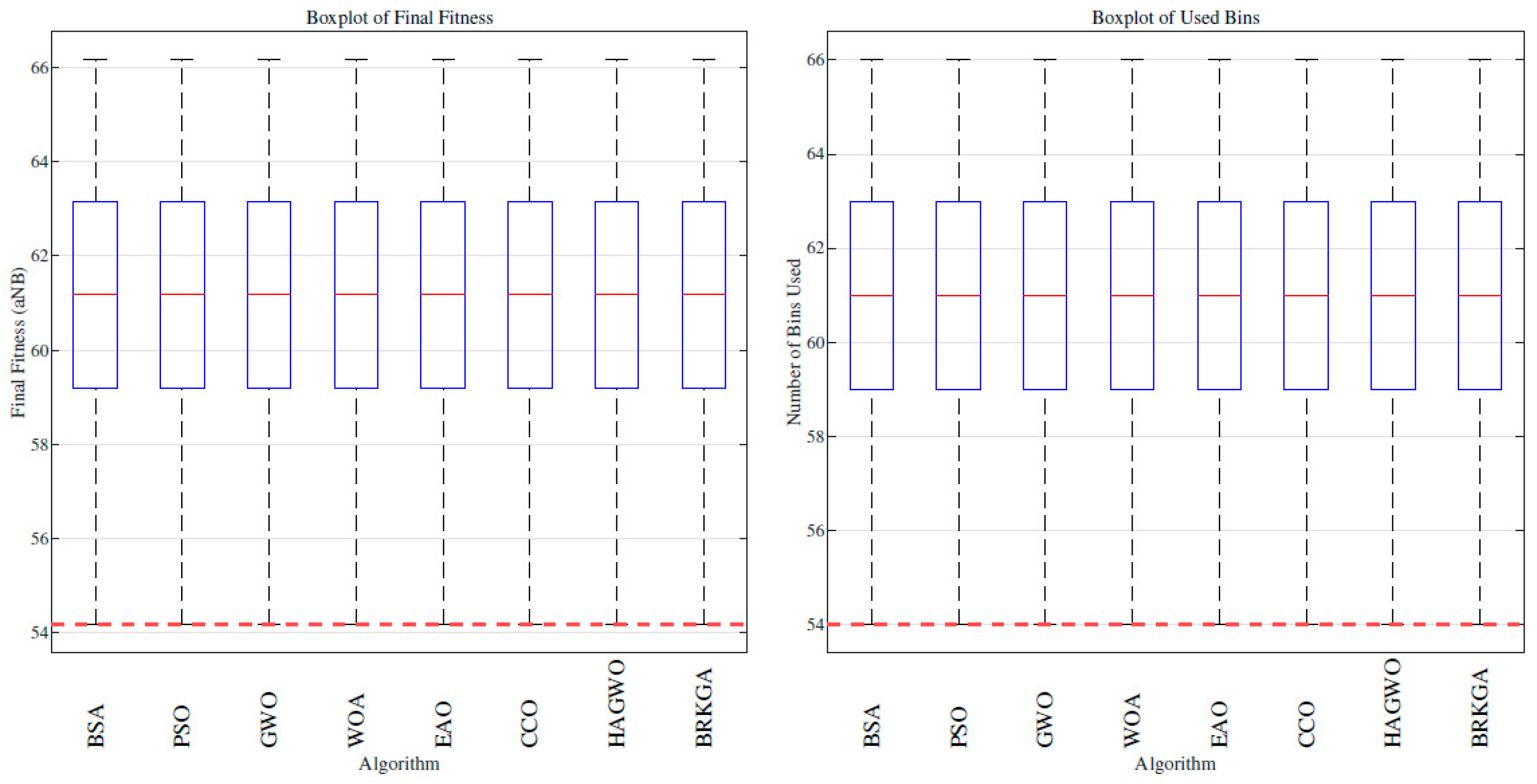
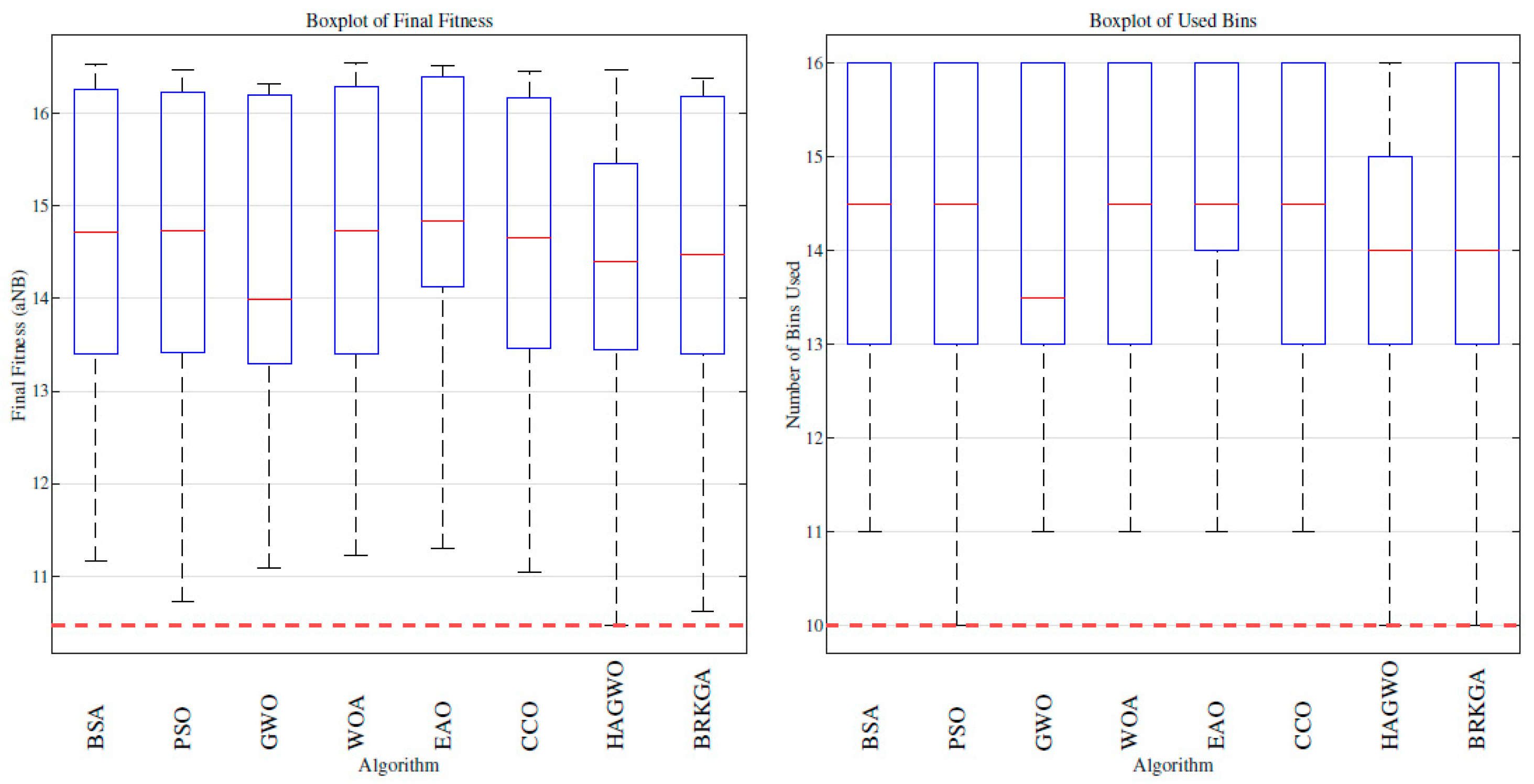
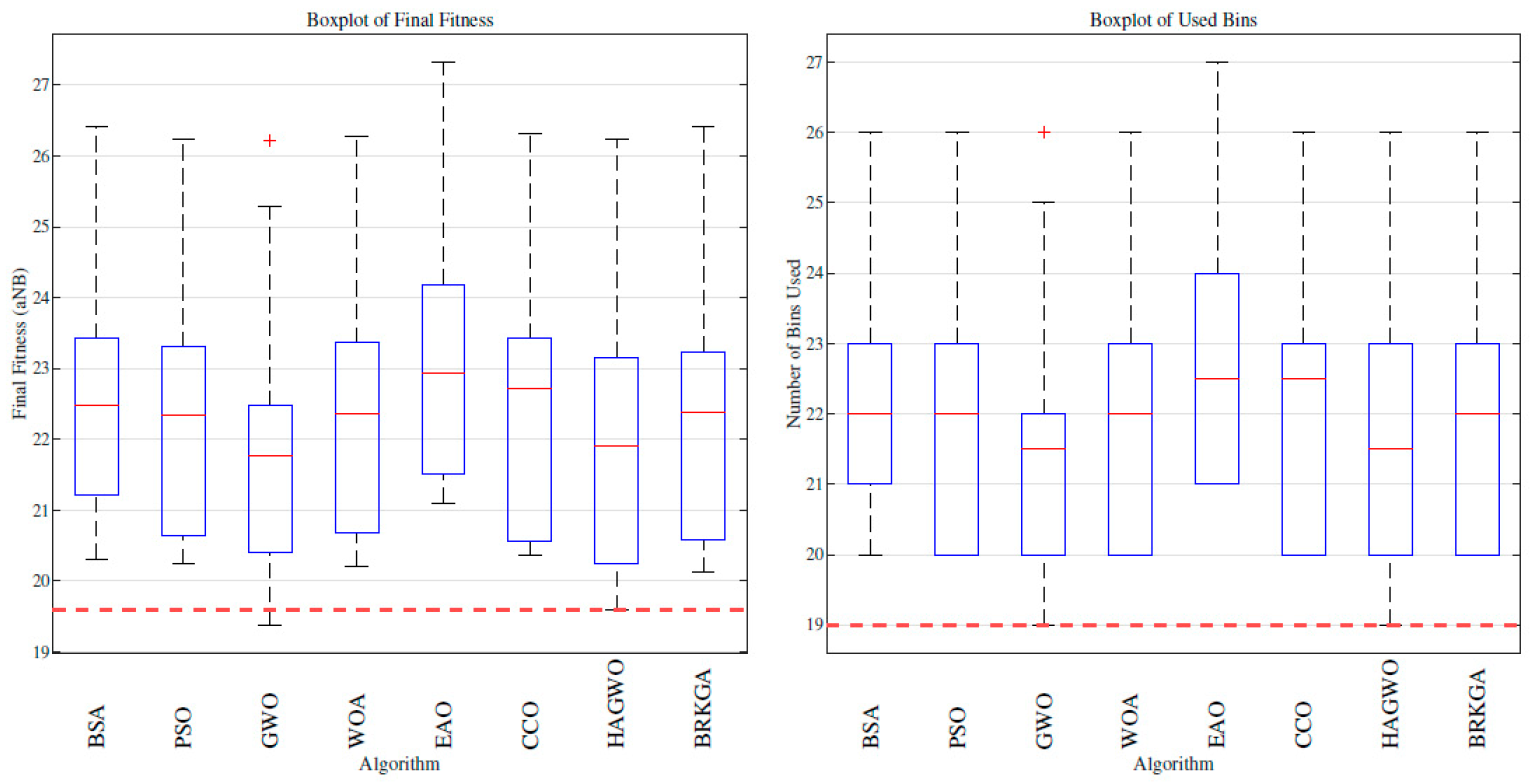
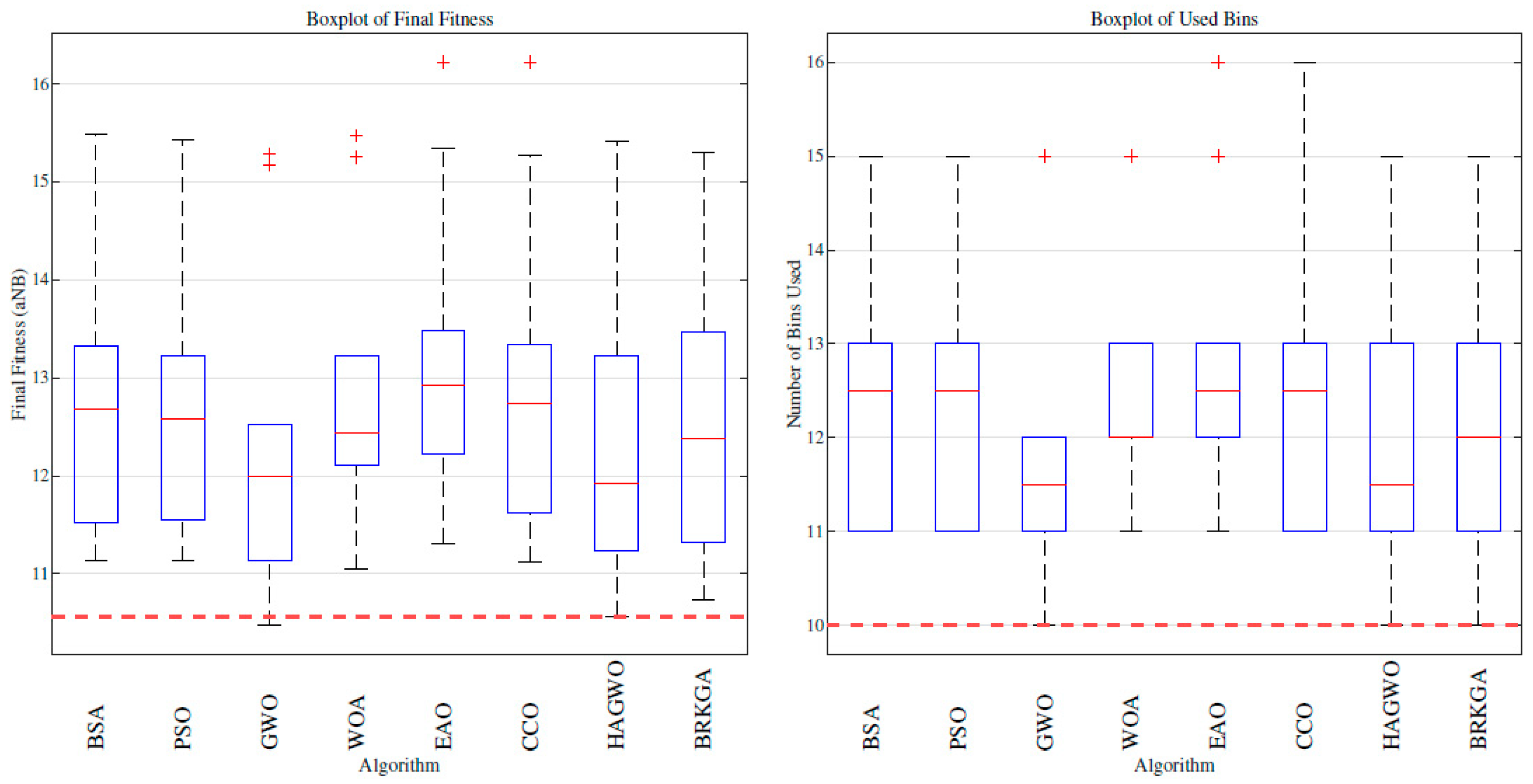
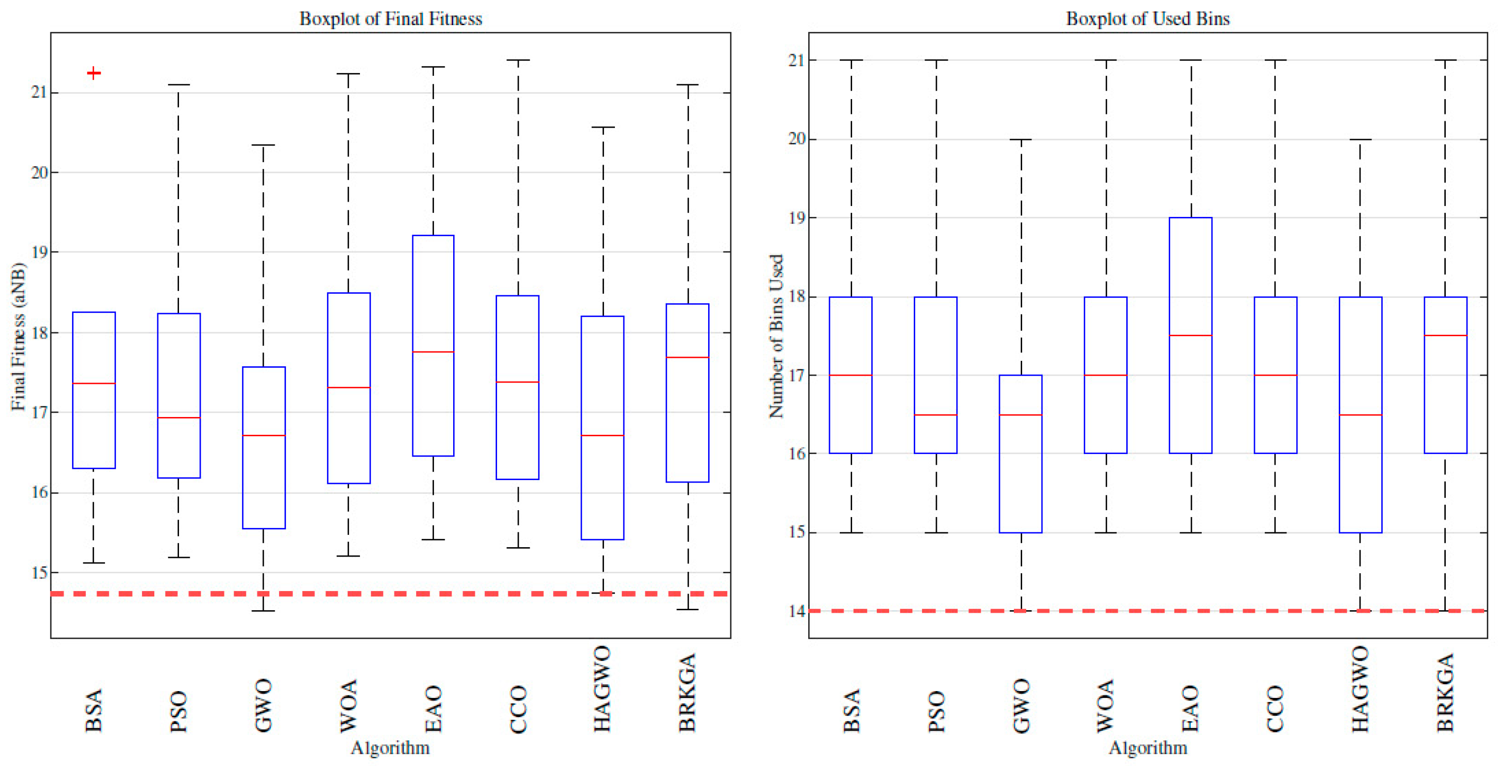
To complement the average performance metrics presented in Table 4, we provide boxplot comparisons of the final fitness (aNB) and the number of used bins (NB) for each of the 16 instance groups (Classes 1–8 at n = 50 and n = 100 ), based on 10 independent runs per algorithm (see Figure A5, Figure A6, Figure A7, Figure A8, Figure A9, Figure A10, Figure A11, Figure A12, Figure A13, Figure A14, Figure A15, Figure A16, Figure A17, Figure A18, Figure A19 and Figure A20).
Across the entire benchmark, HAGWO demonstrates strong stability. In 13 out of 16 instance groups, HAGWO exhibits the narrowest (or jointly narrowest) IQR in at least one of the two boxplots (aNB or NB). This advantage is particularly pronounced in the more challenging classes (1, 2, 3, 6, 7, 8) and becomes even more evident at n = 100 , where increased problem complexity amplifies run-to-run variability in most other algorithms. For instance, in Class 3 ( n = 100 ), HAGWO reduces the IQR of NB by approximately 40% compared to BRKGA, while in Class 7 ( n = 100 ), the number of outliers is reduced from 4–5 (in PSO, BSA, EAO) to nearly zero. HAGWO also consistently produces the fewest and least extreme outliers, confirming that the hybrid adaptive mechanism effectively mitigates stochastic fluctuations and enhances repeatability.
In terms of solution quality, HAGWO ranks in the top two (by median NB) in 9 out of 16 classes and never falls outside the top three. Its overall summed NB across all instances (2967) is the second lowest, trailing GWO (2944) by only 23 bins while outperforming BRKGA (2989), PSO (2999), BSA (3009), CCO (3012), and EAO (3041) by clear margins. In most difficult classes—especially at n = 100 —the median and lower whisker of HAGWO remain very close to those of GWO, often statistically indistinguishable based on visual inspection of the distributions.
Compared with the baseline BRKGA, HAGWO shows a narrower IQR in all 16 classes and fewer outliers in the large majority of cases. It also achieves a lower or equal median NB in 11 classes, resulting in a total improvement of 22 bins (2967 vs. 2989). These consistent gains in both stability and average packing efficiency demonstrate that the proposed hierarchical adversarial-like strategy meaningfully enhances the search process.
On the easier classes (4 and 5 at both n = 50 and n = 100 ), nearly all algorithms converge to nearly identical distributions (overlapping medians, almost identical IQRs, and comparable whiskers), confirming that performance differences diminish when near-optimal packings are readily achievable. HAGWO performs on par with the best methods in these cases, showing no degradation on simpler instances.

5.6.3. Convergence Analysis

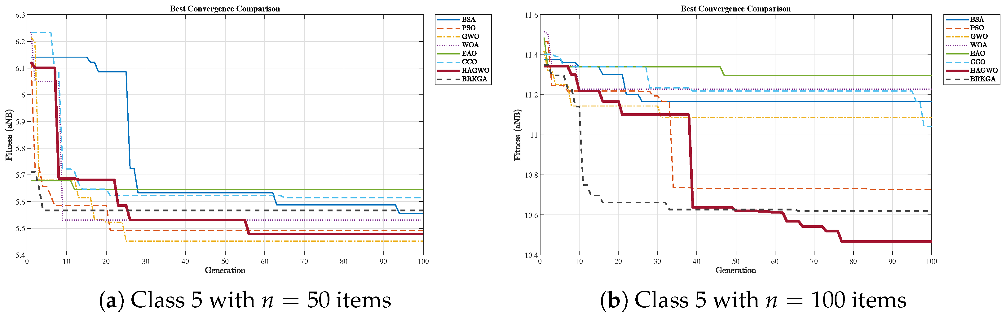
To gain deeper insight into the dynamic behavior of the algorithms, we present convergence curves of the best-found fitness (aNB) over 100 generations for representative instances (Figure 8).
On the easier Class 5 n = 50 instance, most algorithms reach near-optimal regions within the first 30–50 generations. HAGWO demonstrates rapid early improvement, followed by steady refinement until approximately generations 55–60, ultimately stabilizing at one of the lowest and most consistent plateaus. GWO exhibits the steepest initial descent but shows only marginal progress thereafter. BRKGA converges more gradually and stabilizes at a comparatively higher level.
When scaling to n = 100 , the increased problem complexity accentuates behavioral differences. HAGWO maintains steady progress across early, mid, and late stages, achieving the lowest final plateau. This sustained late-stage improvement can be attributed to the hierarchical adversarial-like position updating and adaptive Levy flight perturbation, which maintain population diversity and enable directed escape from local optima even in highly constrained packing landscapes. GWO again shows excellent early convergence but plateaus relatively early with limited late-stage gains. BRKGA maintains a steady but slower trajectory, reaching a competitive yet noticeably higher final level.
Similar trends are observed across other difficult classes (e.g., Classes 1–3 and 6–8 at n = 100 ), where HAGWO frequently continues to refine solutions in generations 60–100, whereas most competitors stagnate earlier. These convergence patterns align closely with the boxplot results: on easier instances, most algorithms achieve similar quality, with HAGWO showing slightly faster and more stable refinement; on larger instances, HAGWO’s ability to continue improving in the late generations provides a clear advantage in both final quality and consistency.
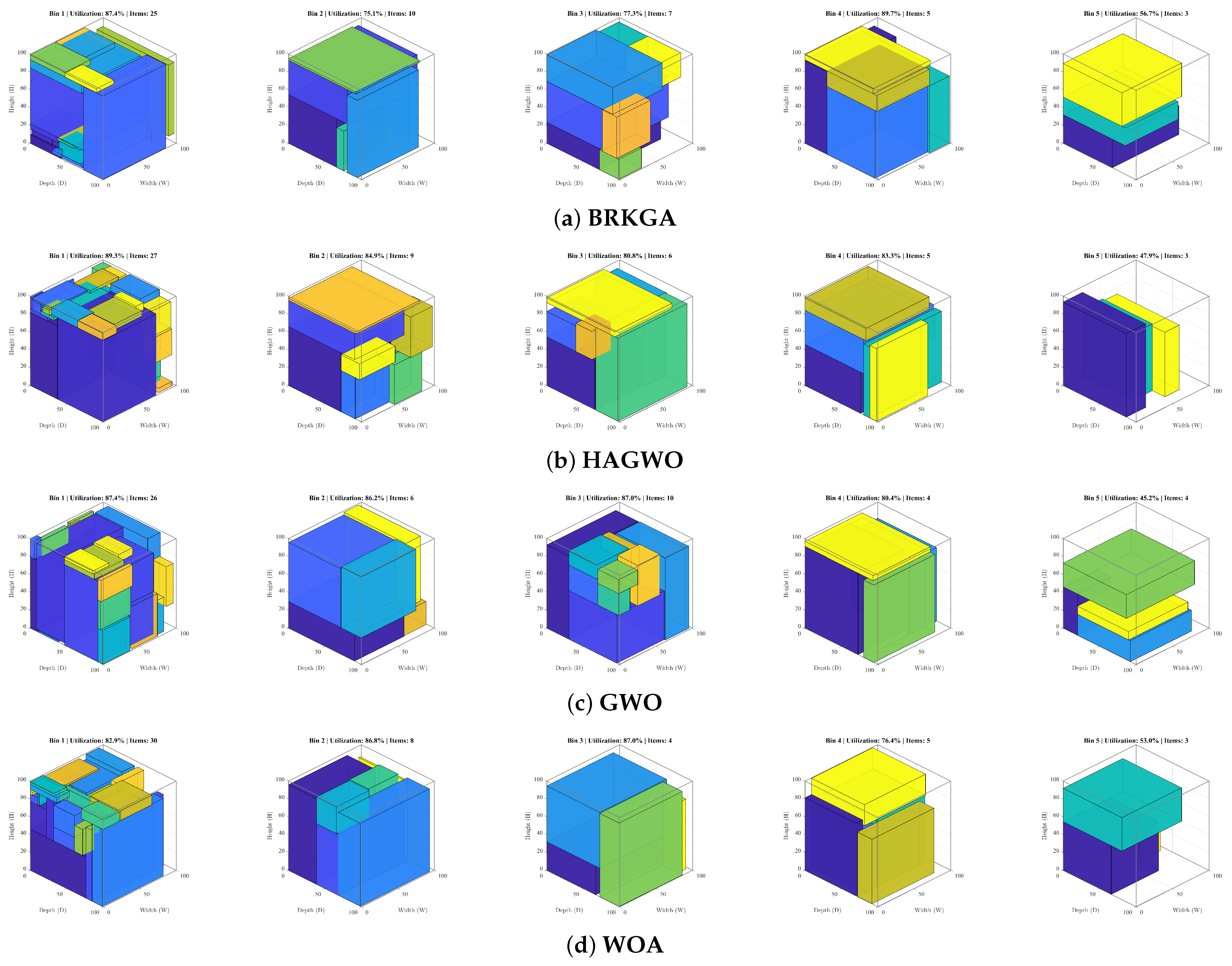
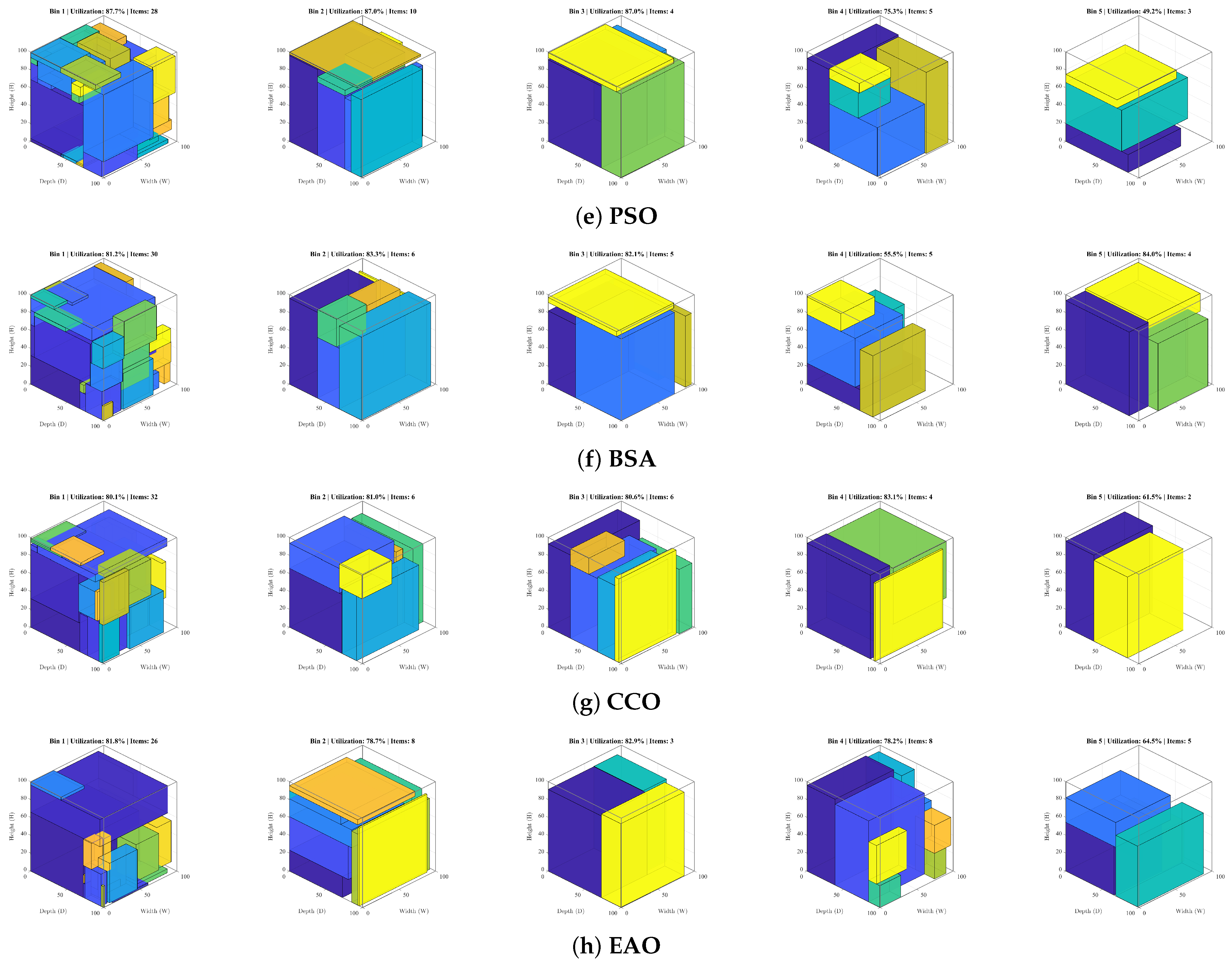
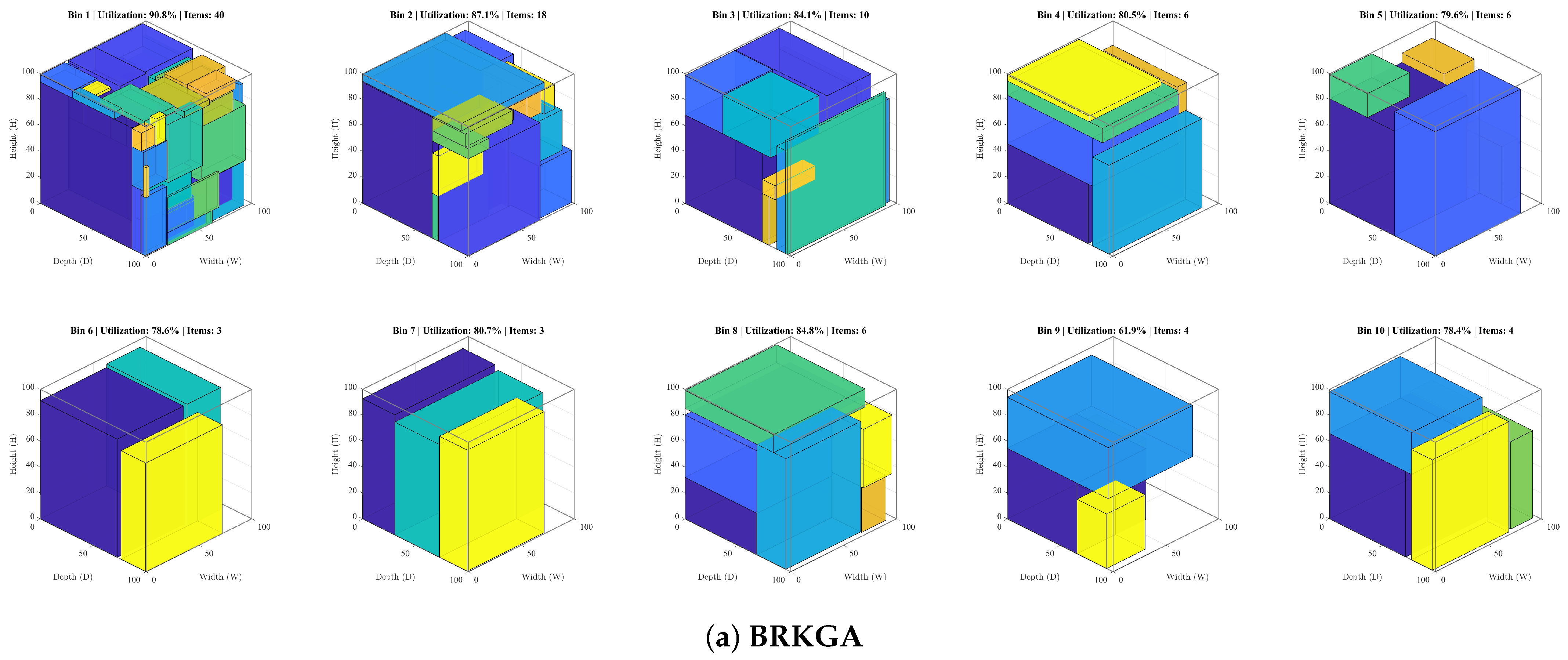
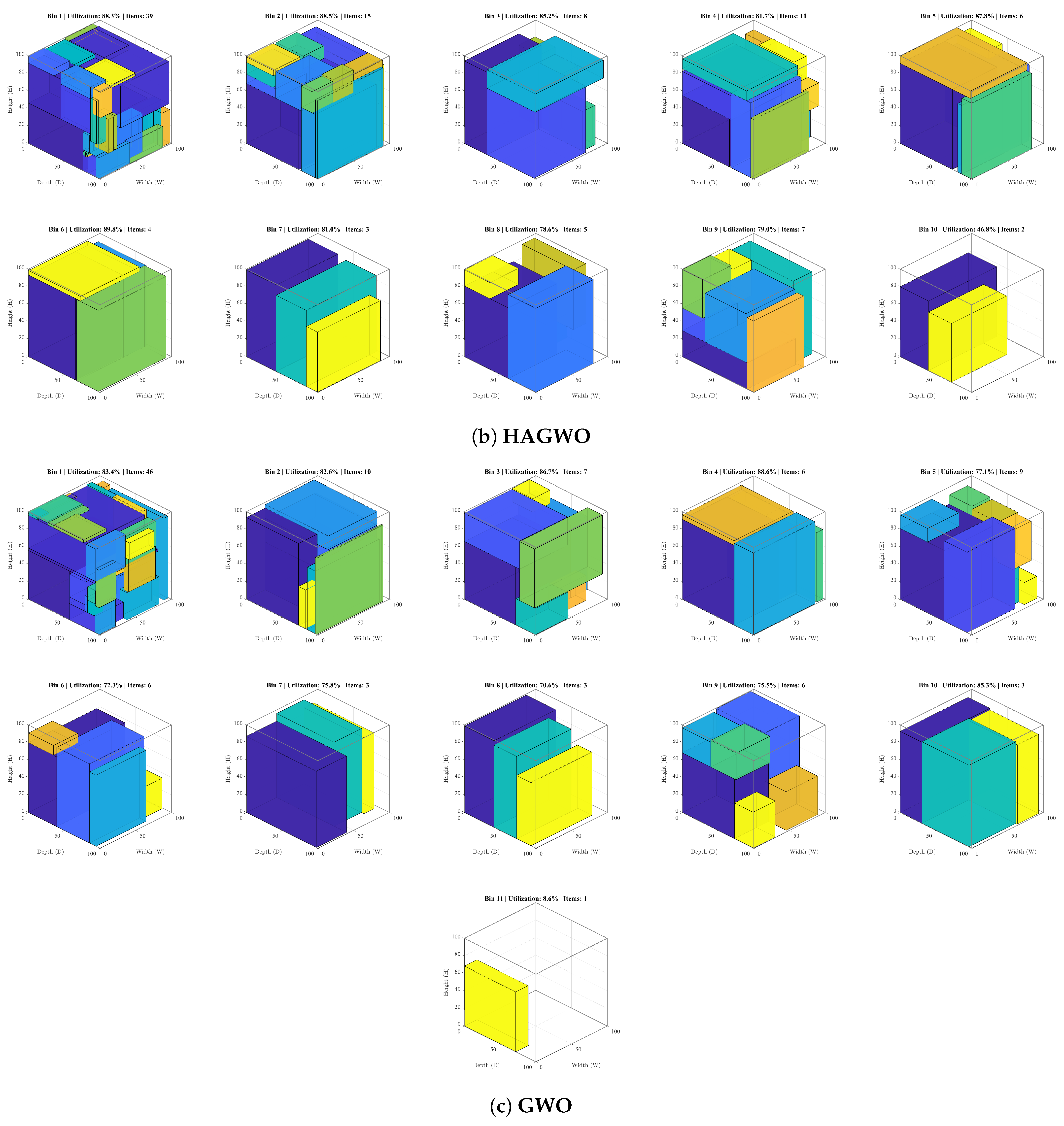
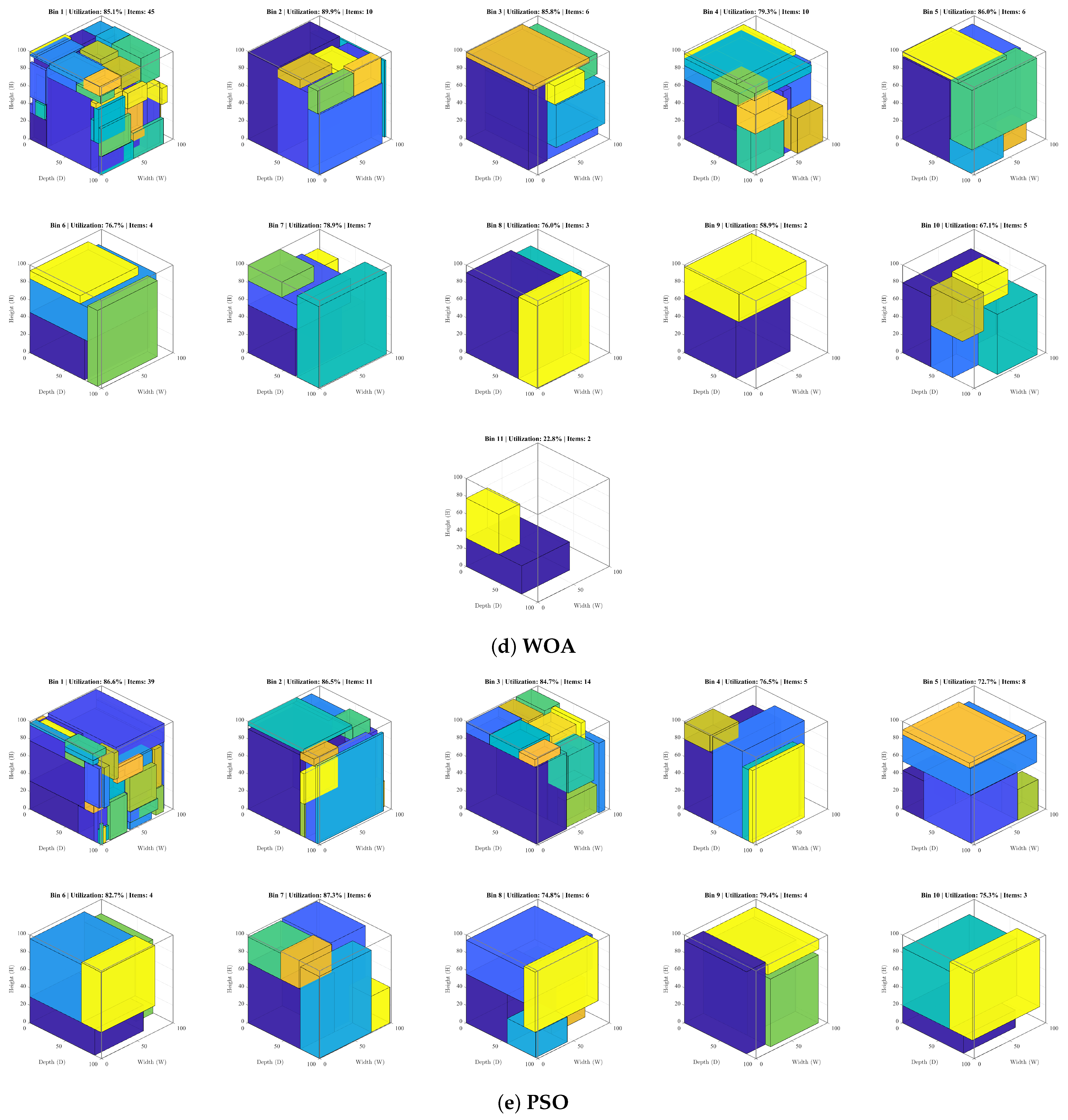
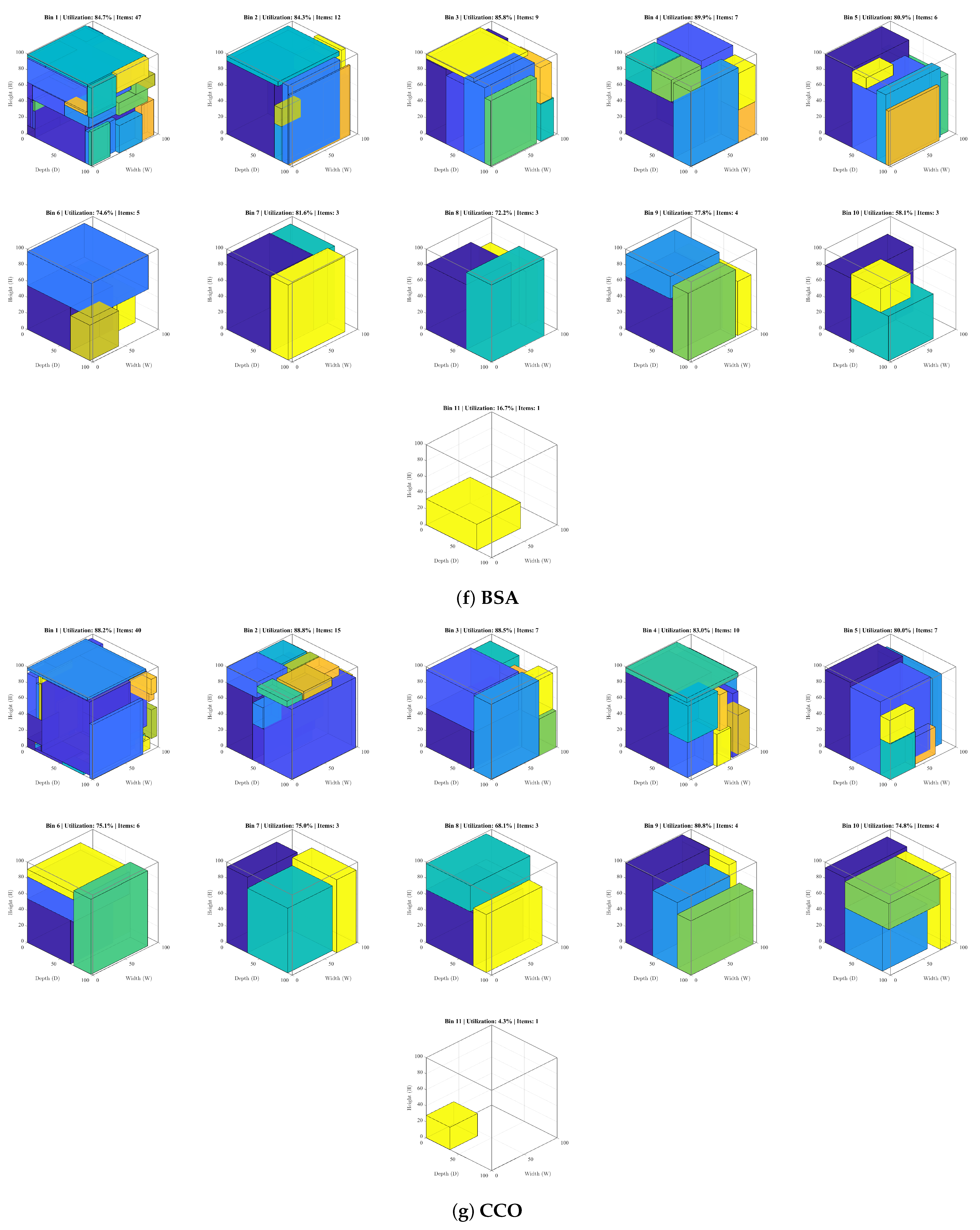
The corresponding three-dimensional visualizations of the best packing solutions for Class 5 ( n = 50 and n = 100 ) are presented in Figure A21 and Figure A22, respectively. HAGWO consistently produces compact and feasible layouts that are visually competitive with BRKGA and GWO while showing fewer irregular gaps compared to other algorithms.

6. Discussion

The experimental results across both continuous benchmark functions and the constrained 3D-SBSBPP reveal the strengths and domain-specific characteristics of the proposed HAGWO, while highlighting meaningful insights into the design of swarm intelligence algorithms for different optimization landscapes.
In continuous optimization (CEC 2017 suite), HAGWO’s superior performance stems directly from its three synergistic mechanisms. Dynamic hierarchical stratification adaptively shifts population composition from exploration-dominant (early emphasis on inferior wolves) to exploitation-dominant phases, effectively preserving diversity and preventing premature convergence. Hierarchical adversarial-like position updating introduces opposition-based learning and directed information flow among stratified groups, enhancing search efficiency and robustness in multimodal, hybrid, and composition landscapes. Adaptive Levy flight perturbation, with linearly decreasing intensity, enables controlled long-range jumps early on and precise local refinement later, allowing robust escape from local optima without disrupting convergence. These innovations collectively address the original GWO’s key limitations—rapid diversity loss and insufficient phase-aware adaptation—leading to statistically significant improvements over GWO and other state-of-the-art methods.
When transferred to the highly constrained 3D-BPP, HAGWO remains highly competitive. As noted in Section 5.6, the original GWO achieves a marginally lower total bin count (2944 vs. 2967), which we attribute to GWO’s simpler, leader-centric hierarchy being particularly robust under strict geometric and non-overlapping constraints where precise local adjustments are critical. Nevertheless, HAGWO consistently outperforms the domain-specific BRKGA in both average packing quality and, particularly, run-to-run stability, suggesting that its core innovations transfer effectively to combinatorial problems when supported by appropriate encoding/decoding strategies and greedy feasibility enforcement.
These domain differences align with the No Free Lunch theorem [32]: no single algorithm can excel universally across all problem landscapes. HAGWO’s strengths in high-dimensional, continuous spaces stem from its ability to maintain long-term population diversity and phase-aware exploration–exploitation balance, making it well-suited for applications such as neural network hyperparameter tuning, complex parameter optimization, or multimodal engineering design. In tightly constrained combinatorial tasks like 3D-BPP, simpler or problem-tailored methods may retain marginal advantages due to their focused exploitation under strict feasibility requirements. The observed trade-off—competitive solution quality with markedly higher stability—highlights the value of hybrid mechanisms that combine global diversity preservation with controlled local refinement.

6.1. Limitations

Several limitations of this study should be acknowledged:
  • Scope of the ablation study: The component-level ablation in Section 5.5 is conducted on the CEC 2017 suite at 30D. While it confirms the individual contributions of the proposed mechanisms, ablation at higher dimensions (50D/100D) and on the 3D-SBSBPP domain, as well as finer-grained parameter sensitivity analysis (stratification ratios, Lévy exponent, disturbance scaling), would provide a more complete picture and is left for future work.
  • Parameter sensitivity: The stratification ratios ( 0.1 , 0.3 , 0.6 ) and ( 0.3 , 0.3 , 0.4 ) , the Levy exponent λ = 1.5 , and the disturbance scaling 0.1 are justified by design principles and established conventions (Section 3.3.1 and Section 3.3.2). However, we acknowledge that a systematic parameter sensitivity analysis—varying each parameter across a grid of values—would strengthen the empirical foundation. The absence of such analysis is a limitation we aim to address in future work.
  • Comparison scope: While our comparison includes diverse metaheuristic paradigms, several recent and competitive GWO variants (e.g., I-GWO [11], EBGWO [15], IAGWO [9], SFGWO [16]) were not included, either because they were published after our experiments began or because their source code was unavailable. A comprehensive benchmark against all recent GWO variants remains future work.
  • 3D-BPP instance coverage: The 3D-BPP experiments were conducted on the standard Martello et al. [2] benchmark set. Real-world packing scenarios may involve additional constraints (weight limits, fragility, loading sequence, irregular item shapes) not captured by this benchmark. The applicability of HAGWO to such extended problem variants requires further investigation.
  • Theoretical analysis: While we provide computational complexity analysis and intuitive explanations for HAGWO’s behavior, formal theoretical analysis (e.g., convergence proofs, convergence rate bounds) remains to be developed.

6.2. Directions for Future Research

To address the limitations identified above and extend HAGWO’s applicability, the following directions merit further investigation:
  • Parameter sensitivity and higher-dimensional ablation: Building on the component-level ablation of Section 5.5, systematically varying each parameter (stratification ratios, Lévy exponent, disturbance scaling) and extending the ablation to 50D/100D and combinatorial domains would provide deeper empirical understanding of their individual and combined effects.
  • Constraint-aware perturbation for discrete optimization: Incorporating feasibility-preserving operators or adaptive penalty mechanisms into the hierarchical update framework would suppress infeasible perturbations in 3D-BPP, potentially narrowing the marginal performance gap with the original GWO observed on certain instance groups.
  • Hybridization with local search: Integrating HAGWO’s global exploration with problem-specific local search heuristics (e.g., EMS-based neighborhood descent) is expected to enhance solution quality on large-scale packing instances where standalone metaheuristics plateau prematurely.
  • Online parameter self-adaptation: Dynamically adjusting Levy flight parameters and disturbance coefficients through real-time diversity metrics—rather than relying on fixed proportional constants—could yield more robust convergence across heterogeneous problem landscapes.
  • Multi-objective and dynamic extensions: Extending HAGWO to multi-objective 3D-BPP variants (e.g., simultaneous minimization of bin count, volume utilization, and carbon footprint) and dynamic scenarios with time-varying item sets remains a promising open avenue.
  • Irregular packing with physical constraints: Generalizing the adversarial hierarchy to handle non-rectangular items subject to center-of-gravity, fragility, and loading-sequence constraints would strengthen real-world applicability in logistics and manufacturing.

7. Conclusions

This paper introduced HAGWO, a novel Hierarchical Adversarial Grey Wolf Optimizer that enhances the original GWO through dynamic hierarchical population stratification, adaptive Levy flight perturbation, and hierarchical adversarial-like position updating. These synergistic mechanisms enable effective diversity maintenance, opposition-based learning, and phase-aware exploration–exploitation balance.
Comprehensive evaluation on the CEC 2017 benchmark suite across multiple dimensions demonstrated HAGWO’s state-of-the-art performance in continuous optimization, achieving the best overall rankings and statistically significant superiority over the original GWO and other leading metaheuristics. When adapted to the strongly NP-hard 3D single-bin-size bin packing problem, HAGWO delivered highly competitive results, outperforming the established BRKGA and most swarm-based methods while exhibiting exceptional stability across all instance groups. We moderated our claims regarding 3D-BPP superiority by acknowledging that the original GWO achieved a marginally lower total bin count, and we discussed how the shared encoding–decoding framework ensures fair comparison.
The work makes three main contributions: (1) a powerful and general-purpose GWO variant with enhanced robustness and search dynamics; (2) rigorous high-dimensional benchmarking confirming clear improvements in continuous spaces; and (3) a successful adaptation to 3D-BPP that reveals valuable insights into continuous-to-discrete transferability and domain-specific trade-offs.
Future work may focus on parameter sensitivity analysis, constraint-aware adaptations for combinatorial problems, hybrid integration with local search or exact methods, and extensions to multi-objective, dynamic, or real-world packing scenarios with irregular items and additional constraints. These directions hold strong potential to advance swarm intelligence in both theoretical and practical contexts.

Author Contributions

S.S.: Investigation, formal analysis, writing—original draft preparation, visualization, and funding acquisition. Z.L.: Formal analysis and visualization. X.H. (Xiaowen Huang): Validation, writing—review and editing, and funding acquisition. X.H. (Xingwang Huang): Methodology, visualization, writing—review and editing, and funding acquisition. All authors have read and agreed to the published version of the manuscript.

Funding

This work was supported in part by the Natural Science Foundation of Xiamen Municipality (3502Z202373035), in part by the Natural Science Foundation of Fujian Province of China (2024J01117, 2025J01347, 2023J01802, 2025H6034), and in part by the Jimei University Startup Fund (ZQ2026008).

Data Availability Statement

All data generated or analyzed during this study are included in this published article. The source code, experimental data, parameter settings, initialization conditions, and random seeds are publicly available at https://github.com/SylvanHuang/HAGWO, accessed on 9 August 2026. The CEC 2017 benchmark functions are available from the IEEE Congress on Evolutionary Computation repository. The 3D-BPP benchmark instances are from the standard dataset by Martello et al. [2].

Conflicts of Interest

The authors declare no conflict of interest.

Appendix A. Numerical Optimization Experiment Results

Table A1. Comparison of HAGWO and other algorithms on the CEC2017 benchmark suite (Dim = 30) (excluding F2).
FunctionMetricHAGWOBSABRKGAGWOPSOWOAEAOCCO
F1Mean9.71e+082.26e+081.09e+091.63e+092.31e+104.87e+094.13e+101.18e+07
Std1.20e+091.49e+084.34e+081.39e+091.05e+103.21e+095.92e+093.93e+07
p-value0.00010.03500.0387< 10 11 < 10 11 < 10 11 < 10 11
Rank32457681
F3Mean9.85e+041.92e+051.52e+057.93e+042.65e+051.46e+051.15e+059.68e+04
Std2.07e+044.08e+043.79e+041.92e+048.68e+043.22e+041.44e+043.99e+04
p-value< 10 11 < 10 11 0.0036< 10 11 < 10 11 0.00930.4528
Rank37618542
F4Mean5.58e+025.90e+027.10e+026.04e+022.90e+037.63e+026.98e+035.93e+02
Std4.25e+013.29e+019.08e+016.51e+011.58e+032.68e+022.38e+031.47e+02
p-value0.0009< 10 11 0.0030< 10 11 < 10 11 < 10 11 0.9263
Rank12638754
F5Mean5.80e+026.91e+026.79e+026.33e+027.29e+027.26e+027.56e+027.82e+02
Std1.89e+011.68e+012.50e+015.85e+013.58e+014.11e+012.61e+015.42e+01
p-value< 10 11 < 10 11 0.0001< 10 11 < 10 11 < 10 11 < 10 11
Rank15427638
F6Mean6.05e+026.07e+026.12e+026.12e+026.35e+026.59e+026.74e+026.67e+02
Std3.28e+002.38e+002.20e+004.21e+008.74e+001.09e+013.98e+001.08e+01
p-value0.0148< 10 11 < 10 11 < 10 11 < 10 11 < 10 11 < 10 11
Rank12345786
F7Mean8.52e+029.76e+021.01e+039.46e+021.30e+031.23e+031.48e+031.72e+03
Std3.38e+012.16e+014.26e+016.40e+012.02e+021.16e+028.20e+012.84e+02
p-value< 10 11 < 10 11 < 10 11 < 10 11 < 10 11 < 10 11 < 10 11
Rank13427658
F8Mean8.84e+029.93e+029.69e+029.37e+021.01e+031.04e+031.12e+031.11e+03
Std1.83e+011.81e+012.59e+015.86e+014.30e+014.31e+013.02e+015.63e+01
p-value< 10 11 < 10 11 0.0001< 10 11 < 10 11 < 10 11 < 10 11
Rank14325687
F9Mean1.87e+032.22e+034.11e+035.15e+039.39e+038.11e+031.50e+041.06e+04
Std6.01e+027.62e+021.69e+032.84e+033.32e+032.55e+031.52e+033.11e+03
p-value0.0285< 10 11 < 10 11 < 10 11 < 10 11 < 10 11 < 10 11
Rank12347685
F10Mean4.59e+037.31e+035.68e+035.77e+036.03e+036.57e+036.55e+035.53e+03
Std9.28e+023.73e+025.05e+021.92e+038.51e+025.65e+022.53e+028.22e+02
p-value< 10 11 < 10 11 0.0117< 10 11 < 10 11 < 10 11 0.0018
Rank18345762
F11Mean1.52e+031.61e+034.25e+032.53e+034.99e+031.86e+038.91e+031.42e+03
Std3.97e+022.32e+022.39e+031.75e+039.38e+034.32e+022.37e+039.82e+01
p-value0.0333< 10 11 < 10 11 < 10 11 0.0007< 10 11 0.5857
Rank23647581
F12                  Mean7.15e+079.13e+061.49e+081.99e+083.07e+092.62e+081.16e+101.53e+07
Std8.19e+076.14e+068.30e+072.83e+082.09e+094.58e+083.02e+091.35e+07
p-value0.00010.00340.0030< 10 11 0.0024< 10 11 0.0003
Rank31457682
F13Mean1.41e+065.39e+054.50e+076.53e+061.09e+091.16e+068.70e+091.48e+05
Std6.68e+061.05e+062.49e+072.40e+072.04e+092.87e+063.86e+092.09e+05
p-value0.0519< 10 11 0.0687< 10 11 0.0017< 10 11 0.2623
Rank42658371
F14Mean4.89e+053.20e+042.06e+064.20e+058.67e+053.56e+058.87e+051.33e+05
Std7.67e+052.23e+042.11e+068.59e+051.95e+064.71e+055.28e+051.46e+05
p-value< 10 11 < 10 11 0.55770.17790.40480.00280.0068
Rank51748362
F15Mean9.49e+056.11e+041.06e+071.66e+069.07e+072.14e+052.43e+089.33e+04
Std1.89e+066.19e+049.27e+063.89e+063.65e+086.96e+053.06e+087.65e+04
p-value0.0087< 10 11 0.46530.65830.3600< 10 11 0.1359
Rank51748362
F16Mean2.49e+033.19e+033.26e+032.77e+033.60e+033.23e+034.89e+033.28e+03
Std3.07e+022.32e+023.27e+025.23e+024.98e+024.01e+025.60e+023.95e+02
p-value< 10 11 < 10 11 0.0285< 10 11 < 10 11 < 10 11 < 10 11
Rank16728543
F17Mean1.99e+032.33e+032.48e+032.14e+032.63e+032.37e+032.86e+032.64e+03
Std1.35e+021.10e+021.95e+022.00e+023.34e+023.01e+022.96e+023.43e+02
p-value< 10 11 < 10 11 0.0140< 10 11 < 10 11 < 10 11 < 10 11
Rank14627583
F18Mean1.84e+067.78e+057.36e+061.86e+061.16e+072.69e+069.16e+061.12e+06
Std1.80e+068.01e+057.21e+062.03e+062.31e+072.35e+067.45e+061.06e+06
p-value0.0015< 10 11 0.73430.00060.1470< 10 11 0.2059
Rank31647582
F19Mean7.67e+053.38e+041.23e+075.58e+056.97e+074.44e+054.32e+086.78e+04
Std1.09e+064.45e+041.47e+075.14e+057.66e+075.99e+054.68e+087.56e+04
p-value< 10 11 < 10 11 0.9918< 10 11 0.1254< 10 11 < 10 11
Rank41738562
F20Mean2.44e+032.74e+032.70e+032.56e+032.74e+032.71e+032.78e+032.87e+03
Std1.64e+021.51e+022.03e+022.64e+022.58e+022.30e+021.15e+022.10e+02
p-value< 10 11 < 10 11 0.0333< 10 11 < 10 11 < 10 11 < 10 11
Rank15426378
F21Mean2.38e+032.49e+032.48e+032.42e+032.52e+032.53e+032.64e+032.58e+03
Std2.06e+011.76e+013.05e+014.59e+015.34e+015.50e+013.38e+015.33e+01
p-value< 10 11 < 10 11 0.0001< 10 11 < 10 11 < 10 11 < 10 11
Rank14326785
F22Mean5.39e+037.78e+035.36e+036.32e+037.34e+037.57e+037.94e+036.65e+03
Std1.84e+031.45e+032.25e+032.74e+031.04e+031.45e+037.02e+021.69e+03
p-value< 10 11 0.45280.17790.00010.0001< 10 11 0.0082
Rank28136754
F23Mean2.75e+032.84e+032.85e+032.85e+033.04e+032.94e+033.55e+033.06e+03
Std2.55e+011.95e+012.62e+017.15e+011.24e+025.71e+011.09e+021.01e+02
p-value< 10 11 < 10 11 < 10 11 < 10 11 < 10 11 < 10 11 < 10 11
Rank12347685
F24                  Mean2.90e+033.03e+033.09e+032.97e+033.24e+033.08e+033.58e+033.14e+03
Std3.10e+012.75e+015.40e+016.61e+018.95e+016.16e+018.76e+019.32e+01
p-value< 10 11 < 10 11 < 10 11 < 10 11 < 10 11 < 10 11 < 10 11
Rank14628573
F25Mean2.97e+032.98e+033.07e+033.00e+034.23e+033.11e+034.70e+032.98e+03
Std2.50e+012.25e+016.73e+014.01e+011.00e+031.23e+025.48e+025.88e+01
p-value0.0132< 10 11 0.0003< 10 11 < 10 11 < 10 11 0.4653
Rank13628754
F26Mean4.55e+035.68e+035.67e+035.03e+037.72e+036.97e+039.71e+038.00e+03
Std3.85e+022.11e+028.53e+025.91e+021.05e+039.57e+025.98e+021.51e+03
p-value< 10 11 < 10 11 0.0028< 10 11 < 10 11 < 10 11 < 10 11
Rank14327685
F27Mean3.24e+033.25e+033.28e+033.27e+033.41e+033.33e+034.21e+033.36e+03
Std1.85e+011.54e+012.61e+013.21e+019.19e+015.32e+011.93e+027.38e+01
p-value0.0598< 10 11 0.0001< 10 11 < 10 11 < 10 11 < 10 11
Rank12437586
F28Mean3.40e+034.08e+033.42e+033.50e+036.49e+033.65e+036.50e+033.74e+03
Std6.68e+011.01e+036.91e+011.48e+021.30e+032.49e+026.09e+026.34e+02
p-value< 10 11 0.46530.0008< 10 11 < 10 11 < 10 11 0.0157
Rank15238674
F29Mean3.78e+034.23e+034.25e+033.97e+034.47e+034.67e+035.99e+034.98e+03
Std1.30e+021.96e+022.36e+021.93e+023.87e+024.13e+029.75e+025.38e+02
p-value< 10 11 < 10 11 0.0003< 10 11 < 10 11 < 10 11 < 10 11
Rank14526783
F30Mean7.46e+062.94e+051.24e+071.24e+071.11e+083.63e+069.85e+081.35e+06
Std5.80e+062.19e+051.20e+077.57e+063.51e+083.02e+066.60e+082.28e+06
p-value< 10 11 0.15890.00570.01400.0044< 10 11 < 10 11
Rank41657382
+/≈/– 6/1/224/1/245/3/210/0/293/1/250/0/295/4/20
Mean rank 2.073.144.903.316.974.866.833.93
Final ranking 12538476
Table A2. Comparison of HAGWO and other algorithms on the CEC2017 benchmark suite (Dim = 50) (excluding F2).
FunctionMetricHAGWOBSABRKGAGWOPSOWOAEAOCCO
F1Mean5.34e+094.41e+095.23e+091.12e+107.62e+102.45e+109.93e+104.41e+09
Std2.96e+091.45e+091.30e+094.12e+092.05e+106.55e+099.26e+093.85e+09
p-value0.09370.7971< 10 11 < 10 11 < 10 11 < 10 11 0.0897
Rank13257684
F3Mean2.71e+053.95e+053.58e+051.83e+055.68e+052.79e+052.18e+053.23e+05
Std5.31e+046.46e+046.03e+042.38e+041.65e+055.92e+042.34e+046.44e+04
p-value< 10 11 < 10 11 < 10 11 < 10 11 0.59990.00010.0053
Rank37618425
F4                    Mean9.25e+021.11e+031.26e+031.41e+031.20e+042.59e+031.77e+041.12e+03
Std2.91e+022.14e+023.32e+027.52e+025.87e+036.77e+022.89e+034.02e+02
p-value0.01570.0004< 10 11 < 10 11 < 10 11 < 10 11 0.0350
Rank12348576
F5Mean6.92e+029.45e+028.87e+027.88e+021.05e+031.04e+031.10e+031.12e+03
Std2.65e+013.72e+014.18e+019.34e+017.21e+018.68e+017.21e+011.11e+02
p-value< 10 11 < 10 11 < 10 11 < 10 11 < 10 11 < 10 11 < 10 11
Rank15427638
F6Mean6.10e+026.23e+026.19e+026.23e+026.62e+026.80e+026.83e+026.77e+02
Std3.98e+004.20e+002.96e+006.60e+001.01e+011.50e+014.19e+008.12e+00
p-value< 10 11 < 10 11 < 10 11 < 10 11 < 10 11 < 10 11 < 10 11
Rank13245786
F7Mean1.04e+031.35e+031.38e+031.26e+032.35e+031.80e+032.26e+032.78e+03
Std7.31e+015.68e+016.48e+011.12e+024.15e+021.55e+021.36e+023.41e+02
p-value< 10 11 < 10 11 < 10 11 < 10 11 < 10 11 < 10 11 < 10 11
Rank13427568
F8Mean1.00e+031.24e+031.17e+031.10e+031.31e+031.32e+031.31e+031.42e+03
Std3.84e+013.32e+015.15e+019.72e+019.24e+018.26e+019.24e+011.09e+02
p-value< 10 11 < 10 11 < 10 11 < 10 11 < 10 11 < 10 11 < 10 11
Rank14326758
F9Mean5.66e+038.24e+031.48e+041.53e+043.77e+042.63e+044.33e+042.92e+04
Std2.19e+032.81e+035.42e+035.13e+031.07e+046.10e+034.54e+036.23e+03
p-value< 10 11 < 10 11 < 10 11 < 10 11 < 10 11 < 10 11 < 10 11
Rank12347586
F10Mean8.01e+031.30e+041.00e+041.01e+041.11e+041.19e+041.19e+048.70e+03
Std1.21e+037.55e+027.31e+023.20e+031.64e+031.07e+035.91e+029.83e+02
p-value< 10 11 0.00280.0687< 10 11 < 10 11 < 10 11 < 10 11
Rank18346572
F11Mean3.66e+037.32e+031.30e+048.68e+031.25e+046.94e+032.69e+042.64e+03
Std1.88e+031.97e+035.91e+034.88e+038.65e+032.99e+035.63e+039.16e+02
p-value< 10 11 < 10 11 < 10 11 < 10 11 < 10 11 < 10 11 0.0087
Rank25764381
F12Mean7.13e+083.32e+081.25e+091.42e+091.44e+102.92e+093.73e+103.10e+08
Std4.60e+081.16e+086.51e+081.13e+097.88e+091.71e+095.79e+096.79e+08
p-value0.00050.00170.0028< 10 11 < 10 11 < 10 11 0.0005
Rank23457681
F13Mean1.06e+084.54e+062.80e+059.04e+068.87e+091.45e+063.37e+103.64e+05
Std1.26e+087.74e+061.63e+056.11e+065.32e+094.55e+059.01e+096.64e+05
p-value< 10 11 < 10 11 < 10 11 < 10 11 0.0001< 10 11 < 10 11
Rank65347281
F14Mean1.05e+062.33e+056.83e+073.65e+064.60e+087.02e+066.76e+098.74e+04
Std1.13e+062.88e+054.62e+071.13e+071.10e+091.75e+072.73e+095.13e+04
p-value0.0140< 10 11 0.07520.0148< 10 11 < 10 11 0.0006
Rank42638571
F15Mean1.34e+074.87e+038.74e+041.15e+079.00e+074.34e+075.11e+074.42e+05
Std2.20e+073.79e+022.88e+052.19e+072.10e+086.52e+074.27e+075.13e+04
p-value< 10 11 0.95900.4528< 10 11 0.1529< 10 11 0.5577
Rank21538674
F16                  Mean3.25e+034.87e+034.60e+033.48e+035.10e+034.49e+036.73e+034.42e+03
Std3.80e+022.27e+025.02e+023.97e+024.33e+025.50e+026.86e+025.19e+02
p-value< 10 11 < 10 11 0.0719< 10 11 < 10 11 < 10 11 < 10 11
Rank15428376
F17Mean3.03e+033.78e+033.85e+033.37e+035.09e+033.86e+034.95e+034.12e+03
Std2.17e+022.12e+023.07e+025.45e+021.09e+034.32e+021.45e+035.31e+02
p-value< 10 11 < 10 11 0.0243< 10 11 < 10 11 < 10 11 < 10 11
Rank14528673
F18Mean5.80e+067.22e+063.85e+071.15e+074.59e+079.83e+066.99e+074.34e+06
Std4.02e+063.41e+062.29e+071.20e+075.68e+076.52e+062.56e+073.06e+06
p-value0.1529< 10 11 0.0937< 10 11 0.0104< 10 11 0.5577
Rank14637582
F19Mean2.59e+068.95e+041.93e+077.85e+063.57e+082.51e+063.10e+094.36e+05
Std2.99e+061.09e+051.18e+071.76e+075.96e+082.99e+061.07e+096.30e+05
p-value< 10 11 < 10 11 0.2452< 10 11 0.6288< 10 11 < 10 11
Rank21548376
F20Mean2.93e+034.03e+033.68e+033.57e+033.77e+033.70e+033.61e+033.81e+03
Std2.62e+022.46e+023.06e+025.80e+023.27e+022.82e+021.57e+023.66e+02
p-value< 10 11 < 10 11 0.0001< 10 11 < 10 11 < 10 11 < 10 11
Rank18324567
F21Mean2.49e+032.70e+032.70e+032.58e+032.86e+032.83e+032.98e+032.90e+03
Std3.64e+013.20e+015.15e+018.91e+015.95e+019.35e+015.02e+019.71e+01
p-value< 10 11 < 10 11 < 10 11 < 10 11 < 10 11 < 10 11 < 10 11
Rank14327685
F22                  Mean9.31e+031.49e+041.21e+041.15e+041.35e+041.30e+041.39e+041.07e+04
Std1.47e+036.28e+027.44e+023.23e+031.88e+031.21e+033.70e+025.91e+02
p-value< 10 11 < 10 11 0.0002< 10 11 < 10 11 < 10 11 0.0002
Rank18537642
F23Mean2.95e+033.15e+033.19e+033.09e+033.61e+033.40e+034.50e+033.53e+03
Std4.18e+013.23e+014.16e+011.09e+022.02e+029.97e+011.96e+021.44e+02
p-value< 10 11 < 10 11 < 10 11 < 10 11 < 10 11 < 10 11 < 10 11
Rank12347586
F24Mean3.09e+033.32e+033.55e+033.26e+033.79e+033.50e+034.17e+033.66e+03
Std4.78e+013.37e+019.49e+011.31e+022.07e+021.02e+021.66e+029.59e+01
p-value< 10 11 < 10 11 < 10 11 < 10 11 < 10 11 < 10 11 < 10 11
Rank12437586
F25Mean3.48e+033.70e+033.75e+033.62e+034.57e+034.81e+035.27e+034.13e+03
Std2.24e+022.08e+022.23e+023.83e+027.84e+027.80e+021.51e+021.66e+02
p-value< 10 11 < 10 11 < 10 11 < 10 11 < 10 11 < 10 11 < 10 11
Rank12346785
F26Mean6.10e+038.12e+038.14e+037.06e+031.46e+041.11e+041.54e+041.33e+04
Std5.64e+022.87e+024.22e+027.83e+021.87e+031.71e+038.07e+021.57e+03
p-value< 10 11 < 10 11 < 10 11 < 10 11 < 10 11 < 10 11 < 10 11
Rank14327685
F27Mean3.58e+033.64e+033.76e+033.71e+034.26e+034.19e+036.30e+034.15e+03
Std9.87e+017.10e+011.10e+021.07e+023.05e+022.63e+023.40e+023.05e+02
p-value0.0064< 10 11 < 10 11 < 10 11 < 10 11 < 10 11 < 10 11
Rank12437685
F28Mean4.23e+036.14e+034.20e+034.86e+031.23e+045.41e+031.14e+045.90e+03
Std3.92e+021.72e+034.04e+024.13e+021.27e+037.95e+021.12e+031.76e+03
p-value< 10 11 0.4653< 10 11 < 10 11 < 10 11 < 10 11 < 10 11
Rank14238576
F29Mean4.48e+035.64e+035.00e+034.86e+038.38e+036.48e+032.36e+046.49e+03
Std2.69e+023.52e+023.62e+023.83e+022.26e+038.71e+021.50e+048.71e+02
p-value< 10 11 < 10 11 < 10 11 < 10 11 < 10 11 < 10 11 < 10 11
Rank14237586
F30Mean1.07e+082.07e+076.54e+071.47e+081.17e+099.41e+074.69e+093.20e+07
Std3.50e+079.75e+064.08e+075.02e+071.25e+094.10e+071.89e+091.48e+07
p-value< 10 11 0.00080.0001< 10 11 0.1470< 10 11 < 10 11
Rank23457186
+/≈/– 6/1/224/1/245/3/210/0/293/1/250/0/295/4/20
Mean rank 1.834.284.523.527.175.037.593.07
Final ranking 13428576
Table A3. Comparison of HAGWO and other algorithms on the CEC2017 benchmark suite (Dim = 100) (excluding F2).
FunctionMetricHAGWOBSABRKGAGWOPSOWOAEAOCCO
F1Mean3.24e+105.20e+102.75e+104.90e+102.70e+111.04e+112.85e+115.75e+10
Std1.03e+109.48e+094.06e+091.09e+105.50e+101.56e+102.05e+101.63e+10
p-value< 10 11 0.02850.0001< 10 11 < 10 11 < 10 11 < 10 11
Rank34258671
F3Mean7.45e+058.59e+058.76e+055.95e+051.24e+069.08e+054.10e+058.50e+05
Std1.07e+051.48e+051.15e+058.26e+042.31e+051.27e+052.35e+041.37e+05
p-value0.00260.00070.0001< 10 11 < 10 11 < 10 11 0.0104
Rank36728514
F4Mean4.17e+038.06e+034.36e+036.97e+038.19e+041.75e+041.12e+051.12e+04
Std1.41e+031.24e+038.68e+022.69e+032.24e+046.63e+031.27e+046.48e+03
p-value< 10 11 0.68840.0002< 10 11 < 10 11 < 10 11 < 10 11
Rank14238576
F5Mean1.10e+031.70e+031.56e+031.25e+031.97e+031.88e+031.89e+031.94e+03
Std6.44e+017.27e+017.43e+011.19e+021.53e+021.45e+025.41e+011.71e+02
p-value< 10 11 < 10 11 < 10 11 < 10 11 < 10 11 < 10 11 < 10 11
Rank15428637
F6Mean6.25e+026.54e+026.31e+026.40e+026.99e+026.98e+026.93e+026.89e+02
Std5.36e+004.98e+003.34e+005.40e+001.06e+011.36e+012.83e+007.11e+00
p-value< 10 11 < 10 11 < 10 11 < 10 11 < 10 11 < 10 11 < 10 11
Rank15248763
F7Mean1.96e+032.81e+032.68e+032.43e+036.89e+033.60e+034.47e+036.41e+03
Std1.50e+021.16e+021.36e+022.74e+029.55e+022.41e+022.03e+026.44e+02
p-value< 10 11 < 10 11 < 10 11 < 10 11 < 10 11 < 10 11 < 10 11
Rank14328567
F8                    Mean1.37e+031.98e+031.87e+031.58e+032.37e+032.17e+032.20e+032.26e+03
Std6.63e+016.93e+017.46e+011.54e+021.06e+021.77e+023.82e+011.33e+02
p-value< 10 11 < 10 11 < 10 11 < 10 11 < 10 11 < 10 11 < 10 11
Rank15428637
F9Mean2.21e+045.03e+045.72e+045.03e+041.45e+058.16e+048.05e+047.26e+04
Std6.37e+037.83e+031.05e+041.09e+042.69e+041.66e+046.08e+031.17e+04
p-value< 10 11 < 10 11 < 10 11 < 10 11 < 10 11 < 10 11 < 10 11
Rank13628745
F10Mean1.76e+043.02e+042.44e+042.60e+042.79e+042.72e+042.77e+041.91e+04
Std2.54e+031.12e+031.12e+037.30e+033.32e+031.75e+035.92e+029.83e+02
p-value< 10 11 < 10 11 < 10 11 < 10 11 < 10 11 < 10 11 0.0050
Rank16348572
F11Mean9.18e+041.61e+051.41e+059.88e+043.75e+051.32e+052.12e+051.05e+05
Std2.54e+042.94e+044.63e+041.75e+041.02e+053.77e+042.45e+044.02e+04
p-value< 10 11 < 10 11 0.1470< 10 11 < 10 11 < 10 11 0.2712
Rank15428673
F12Mean6.72e+094.76e+097.33e+091.05e+101.10e+113.20e+101.83e+116.03e+09
Std4.64e+091.39e+091.68e+094.61e+092.83e+101.47e+101.78e+104.74e+09
p-value0.19860.00300.0018< 10 11 < 10 11 < 10 11 0.5304
Rank23458671
F13Mean4.24e+088.26e+076.61e+089.82e+081.61e+104.39e+094.05e+102.79e+07
Std6.32e+084.87e+072.59e+089.41e+086.13e+093.02e+095.94e+099.89e+07
p-value0.0001< 10 11 0.0087< 10 11 < 10 11 < 10 11 < 10 11
Rank23458671
F14Mean7.84e+061.16e+075.28e+078.15e+065.90e+071.36e+072.70e+078.59e+06
Std3.54e+065.30e+062.98e+073.80e+063.79e+077.65e+061.25e+074.49e+06
p-value0.0087< 10 11 0.9426< 10 11 < 10 11 < 10 11 0.5038
Rank13628457
F15Mean9.30e+072.44e+062.30e+083.73e+087.91e+096.53e+081.99e+103.47e+06
Std1.46e+082.47e+061.07e+084.81e+083.94e+097.35e+083.77e+091.04e+07
p-value< 10 11 < 10 11 0.0034< 10 11 0.0009< 10 11 < 10 11
Rank23458671
F16Mean6.27e+031.03e+049.18e+036.97e+031.22e+041.07e+041.76e+048.36e+03
Std8.09e+024.80e+025.91e+021.23e+031.59e+031.01e+032.09e+031.14e+03
p-value< 10 11 < 10 11 0.0207< 10 11 < 10 11 < 10 11 < 10 11
Rank15428673
F17Mean4.90e+037.29e+037.81e+035.88e+031.58e+051.02e+042.71e+067.23e+03
Std5.19e+023.66e+021.24e+031.04e+031.93e+057.48e+032.25e+061.12e+03
p-value< 10 11 < 10 11 0.0001< 10 11 < 10 11 < 10 11 < 10 11
Rank14528673
F18Mean7.26e+061.57e+075.25e+071.07e+077.99e+071.53e+076.61e+071.30e+07
Std4.61e+067.43e+063.34e+076.28e+069.44e+076.93e+063.90e+077.20e+06
p-value< 10 11 < 10 11 0.0157< 10 11 < 10 11 < 10 11 0.0008
Rank13628457
F19Mean9.48e+074.16e+061.80e+082.02e+086.25e+094.09e+081.91e+107.67e+06
Std1.97e+082.85e+067.03e+072.06e+084.06e+094.12e+083.34e+091.23e+07
p-value< 10 11 0.00010.0064< 10 11 < 10 11 < 10 11 < 10 11
Rank23458671
F20                  Mean5.17e+037.64e+036.52e+035.91e+037.66e+036.58e+036.35e+036.17e+03
Std7.31e+022.91e+025.77e+021.34e+037.10e+026.38e+022.04e+025.78e+02
p-value< 10 11 < 10 11 0.0822< 10 11 < 10 11 < 10 11 < 10 11
Rank16438527
F21Mean2.92e+033.42e+033.44e+033.10e+034.10e+033.79e+034.48e+034.01e+03
Std7.22e+014.81e+017.68e+011.82e+021.62e+021.91e+021.08e+021.85e+02
p-value< 10 11 < 10 11 < 10 11 < 10 11 < 10 11 < 10 11 < 10 11
Rank14528673
F22Mean1.97e+043.20e+042.60e+042.66e+042.92e+042.89e+043.06e+042.09e+04
Std2.21e+031.07e+031.12e+037.20e+033.51e+032.02e+035.05e+021.50e+03
p-value< 10 11 < 10 11 < 10 11 < 10 11 < 10 11 < 10 11 0.0039
Rank18346572
F23Mean3.46e+033.86e+033.71e+033.77e+035.13e+034.48e+036.99e+034.84e+03
Std9.49e+014.01e+017.11e+011.65e+022.91e+021.51e+023.01e+022.58e+02
p-value< 10 11 < 10 11 < 10 11 < 10 11 < 10 11 < 10 11 < 10 11
Rank14238576
F24Mean4.10e+034.49e+034.49e+034.49e+036.97e+035.56e+035.13e+036.06e+03
Std1.31e+027.49e+019.45e+011.61e+024.58e+021.11e+034.01e+023.29e+02
p-value< 10 11 < 10 11 < 10 11 < 10 11 < 10 11 < 10 11 < 10 11
Rank12348657
F25Mean6.01e+037.93e+036.96e+036.70e+034.16e+047.40e+032.66e+047.40e+03
Std9.03e+027.93e+021.11e+038.62e+027.56e+037.93e+022.59e+033.55e+03
p-value< 10 11 < 10 11 < 10 11 < 10 11 0.0005< 10 11 < 10 11
Rank14328576
F26Mean1.41e+041.86e+041.85e+041.75e+044.12e+041.01e+044.98e+043.55e+04
Std1.27e+039.26e+021.32e+032.09e+037.56e+031.97e+033.04e+034.20e+03
p-value< 10 11 < 10 11 < 10 11 < 10 11 < 10 11 < 10 11 < 10 11
Rank14328576
F27Mean4.01e+034.30e+034.12e+034.30e+034.26e+035.38e+031.19e+044.93e+03
Std1.10e+021.96e+029.82e+012.14e+022.95e+024.37e+021.21e+034.69e+02
p-value< 10 11 0.0001< 10 11 < 10 11 < 10 11 < 10 11 < 10 11
Rank13245687
F28Mean7.88e+031.23e+041.01e+049.40e+036.06e+031.34e+041.19e+041.48e+04
Std1.49e+031.84e+032.40e+031.62e+039.34e+021.62e+031.97e+033.90e+03
p-value< 10 11 0.00150.0003< 10 11 < 10 11 < 10 11 < 10 11
Rank36451728
F29Mean8.13e+031.09e+049.41e+039.17e+034.46e+041.37e+041.52e+041.17e+04
Std6.39e+025.45e+021.92e+038.49e+024.88e+042.44e+031.04e+042.00e+03
p-value< 10 11 0.00020.0001< 10 11 < 10 11 < 10 11 < 10 11
Rank15328674
F30Mean9.30e+081.28e+086.18e+081.56e+091.34e+101.94e+093.51e+101.04e+08
Std9.85e+086.67e+072.75e+081.16e+093.96e+091.55e+095.96e+096.83e+07
p-value< 10 11 0.34930.0656< 10 11 0.0044< 10 11 < 10 11
Rank27348561
+/≈/– 1/1/270/2/272/3/242/1/260/2/271/0/283/3/23
Mean rank 1.624.623.793.457.175.346.073.93
Final ranking 17328564
Figure A1. Convergence curves of HAGWO and other algorithms on unimodal (F1, F3), multimodal (F4–F10), and a part of hybrid functions (F11–F16) from the CEC2017 benchmark suite ( D i m = 30 ).
Mathematics 14 03011 g0a1
Figure A2. Convergence curves of HAGWO and other algorithms on the remaining hybrid (F17–F20) and composition functions (F21–F30) from the CEC2017 benchmark suite ( D i m = 30 ).
Mathematics 14 03011 g0a2
Figure A3. Boxplots of HAGWO and competing algorithms on unimodal (F1, F3), multimodal (F4–F10), and hybrid functions (F11–F16) from the CEC2017 benchmark suite ( D i m = 30 ).
Mathematics 14 03011 g0a3
Figure A4. Boxplots of HAGWO and other algorithms on the remaining hybrid (F17–F20) and composition functions (F21–F30) from the CEC2017 benchmark suite ( D i m = 30 ).
Mathematics 14 03011 g0a4
Figure A5. Boxplots comparing the average number of bins (aNB) and the best number of bins (NB) achieved by the algorithms on Class 1 with n = 50 items (10 independent runs each). Lower values and narrower boxes signify better solution quality and greater stability.
Mathematics 14 03011 g0a5
Figure A6. Boxplots comparing the average number of bins (aNB) and the best number of bins (NB) achieved by the algorithms on Class 2 with n = 50 items (10 independent runs each). Lower values and narrower boxes signify better solution quality and greater stability.
Mathematics 14 03011 g0a6
Figure A7. Boxplots comparing the average number of bins (aNB) and the best number of bins (NB) achieved by the algorithms on Class 3 with n = 50 items (10 independent runs each). Lower values and narrower boxes signify better solution quality and greater stability.
Mathematics 14 03011 g0a7
Figure A8. Boxplots comparing the average number of bins (aNB) and the best number of bins (NB) achieved by the algorithms on Class 4 with n = 50 items (10 independent runs each). Lower values and narrower boxes signify better solution quality and greater stability.
Mathematics 14 03011 g0a8
Figure A9. Boxplots comparing the average number of bins (aNB) and the best number of bins (NB) achieved by the algorithms on Class 5 with n = 50 items (10 independent runs each). Lower values and narrower boxes signify better solution quality and greater stability.
Mathematics 14 03011 g0a9
Figure A10. Boxplots comparing the average number of bins (aNB) and the best number of bins (NB) achieved by the algorithms on Class 6 with n = 50 items (10 independent runs each). Lower values and narrower boxes signify better solution quality and greater stability.
Mathematics 14 03011 g0a10
Figure A11. Boxplots comparing the average number of bins (aNB) and the best number of bins (NB) achieved by the algorithms on Class 7 with n = 50 items (10 independent runs each). Lower values and narrower boxes signify better solution quality and greater stability.
Mathematics 14 03011 g0a11
Figure A12. Boxplots comparing the average number of bins (aNB) and the best number of bins (NB) achieved by the algorithms on Class 8 with n = 50 items (10 independent runs each). Lower values and narrower boxes signify better solution quality and greater stability.
Mathematics 14 03011 g0a12
Figure A13. Boxplots comparing the average number of bins (aNB) and the best number of bins (NB) achieved by the algorithms on Class 1 with n = 100 items (10 independent runs each). Lower values and narrower boxes signify better solution quality and greater stability.
Mathematics 14 03011 g0a13
Figure A14. Boxplots comparing the average number of bins (aNB) and the best number of bins (NB) achieved by the algorithms on Class 2 with n = 100 items (10 independent runs each). Lower values and narrower boxes signify better solution quality and greater stability.
Mathematics 14 03011 g0a14
Figure A15. Boxplots comparing the average number of bins (aNB) and the best number of bins (NB) achieved by the algorithms on Class 3 with n = 100 items (10 independent runs each). Lower values and narrower boxes signify better solution quality and greater stability.
Mathematics 14 03011 g0a15
Figure A16. Boxplots comparing the average number of bins (aNB) and the best number of bins (NB) achieved by the algorithms on Class 4 with n = 100 items (10 independent runs each). Lower values and narrower boxes signify better solution quality and greater stability.
Mathematics 14 03011 g0a16
Figure A17. Boxplots comparing the average number of bins (aNB) and the best number of bins (NB) achieved by the algorithms on Class 5 with n = 100 items (10 independent runs each). Lower values and narrower boxes signify better solution quality and greater stability.
Mathematics 14 03011 g0a17
Figure A18. Boxplots comparing the average number of bins (aNB) and the best number of bins (NB) achieved by the algorithms on Class 6 with n = 100 items (10 independent runs each). Lower values and narrower boxes signify better solution quality and greater stability.
Mathematics 14 03011 g0a18
Figure A19. Boxplots comparing the average number of bins (aNB) and the best number of bins (NB) achieved by the algorithms on Class 7 with n = 100 items (10 independent runs each). Lower values and narrower boxes signify better solution quality and greater stability.
Mathematics 14 03011 g0a19
Figure A20. Boxplots comparing the average number of bins (aNB) and the best number of bins (NB) achieved by the algorithms on Class 8 with n = 100 items (10 independent runs each). Lower values and narrower boxes signify better solution quality and greater stability.
Mathematics 14 03011 g0a20
Figure A21. Best packing visualizations of (a) BRKGA, (b) HAGWO, (c) GWO, (d) WOA, (e) PSO, (f) BSA, (g) CCO, and (h) on Class 5 with n = 50 (10 independent runs per algorithm). All used bins from the best solution are shown.
Mathematics 14 03011 g0a21aMathematics 14 03011 g0a21b
Figure A22. Best packing visualizations of BRKGA, HAGWO, GWO, WOA, PSO, BSA, CCO and EAO on Class 5 with n = 100 (10 independent runs per algorithm). All used bins from the best solution are shown.
Mathematics 14 03011 g0a22aMathematics 14 03011 g0a22bMathematics 14 03011 g0a22cMathematics 14 03011 g0a22dMathematics 14 03011 g0a22e

References

  1. Wu, G.; Mallipeddi, R.; Suganthan, P.N. Problem Definitions and Evaluation Criteria for the CEC 2017 Competition on Constrained Real-Parameter Optimization; Technical Report No. 9; National University of Defense Technology: Changsha, China; Kyungpook National University: Daegu, Republic of Korea; Nanyang Technological University: Singapore, 2017; Available online: https://www.researchgate.net/publication/317228117 (accessed on 9 August 2026).
  2. Martello, S.; Pisinger, D.; Vigo, D. The three-dimensional bin packing problem. Oper. Res. 2000, 48, 256–267. [Google Scholar] [CrossRef] [Scilit]
  3. Kennedy, J.; Eberhart, R. Particle Swarm Optimization. In Proceedings of ICNN’95—International Conference on Neural Networks; IEEE: Piscataway, NJ, USA, 1995; Volume 4, pp. 1942–1948. [Google Scholar] [CrossRef] [Scilit]
  4. Storn, R.; Price, K. Differential Evolution – A Simple and Efficient Heuristic for Global Optimization over Continuous Spaces. J. Glob. Optim. 1997, 11, 341–359. [Google Scholar] [CrossRef] [Scilit]
  5. Karaboga, D.; Basturk, B. A powerful and efficient algorithm for numerical function optimization: Artificial bee colony (ABC) algorithm. J. Glob. Optim. 2007, 39, 459–471. [Google Scholar] [CrossRef] [Scilit]
  6. Mirjalili, S.; Lewis, A. The Whale Optimization Algorithm. Adv. Eng. Softw. 2016, 95, 51–67. [Google Scholar] [CrossRef] [Scilit]
  7. Wang, C.H.; Hu, K.; Wu, X.; Ou, Y. Rethinking Metaheuristics: Unveiling the Myth of “Novelty” in Metaheuristic Algorithms. Mathematics 2025, 13, 2158. [Google Scholar] [CrossRef] [Scilit]
  8. Ferhat, A.; Zitouni, F.; Lakbichi, R.; Limane, A.; Harous, S. Measures of exploration and exploitation rates in MAs: Classification, comparison, and convergence analysis. Memetic Comput. 2025, 17, 37. [Google Scholar] [CrossRef] [Scilit]
  9. Yu, M.; Xu, J.; Liang, W.; Qiu, Y.; Bao, S.; Tang, L. Improved multi-strategy adaptive Grey Wolf Optimization for practical engineering applications and high-dimensional problem solving. Artif. Intell. Rev. 2024, 57, 277. [Google Scholar] [CrossRef] [Scilit]
  10. Mirjalili, S.; Mirjalili, S.M.; Lewis, A. Grey Wolf Optimizer. Adv. Eng. Softw. 2014, 69, 46–61. [Google Scholar] [CrossRef] [Scilit]
  11. Nadimi-Shahraki, M.H.; Taghian, S.; Mirjalili, S. An improved grey wolf optimizer for solving engineering problems. Expert Syst. Appl. 2021, 166, 113917. [Google Scholar] [CrossRef] [Scilit]
  12. Wang, L.; Du, H.; Zhang, Z.; Hu, G.; Mirjalili, S.; Khodadadi, N.; Hussien, A.G.; Liao, Y.; Zhao, W. Tianji’s horse racing optimization (THRO): A new metaheuristic inspired by ancient wisdom and its engineering optimization applications. Artif. Intell. Rev. 2025, 58, 282. [Google Scholar] [CrossRef] [Scilit]
  13. Yang, X.S. Firefly algorithm, Levy flights and global optimization. In Research and Development in Intelligent Systems XXVI; Springer: London, UK, 2010; pp. 209–218. [Google Scholar] [CrossRef] [Scilit]
  14. Gonçalves, J.F.; Resende, M.G. A biased random key genetic algorithm for 2D and 3D bin packing problems. Int. J. Prod. Econ. 2013, 145, 500–510. [Google Scholar] [CrossRef] [Scilit]
  15. Jiang, J.; Zhao, Z.; Li, W.; Li, K. An enhanced Grey Wolf Optimizer with elite inheritance and balance search mechanisms. arXiv 2024, arXiv:2404.06524. [Google Scholar]
  16. Zhang, J.; Wu, Z.; Wang, L.; Zhang, Y.; Liu, Z. An improved grey wolf optimization algorithm based on scale-free network topology. Heliyon 2024, 10, e35958. [Google Scholar] [CrossRef] [Scilit] [PubMed]
  17. Jain, A.; Nagar, S.; Singh, P.K.; Dhar, J. A hybrid learning-based genetic and grey-wolf optimizer for global optimization. Soft Comput. 2023, 27, 4713–4759. [Google Scholar] [CrossRef] [Scilit]
  18. Wang, T.L.; Gu, S.W.; Liu, R.J.; Chen, L.Q.; Wang, Z.; Zeng, Z.Q. Cuckoo catfish optimizer: A new meta-heuristic optimization algorithm. Artif. Intell. Rev. 2025, 58, 326. [Google Scholar] [CrossRef] [Scilit]
  19. Rodan, A.; Al-Tamimi, A.K.; Al-Alnemer, L.; Mirjalili, S.; Tiňo, P. Enzyme action optimizer: A novel bio-inspired optimization algorithm. J. Supercomput. 2025, 81, 686. [Google Scholar] [CrossRef] [Scilit]
  20. Derrac, J.; García, S.; Molina, D.; Herrera, F. A Practical Tutorial on the Use of Nonparametric Statistical Tests as a Methodology for Comparing Evolutionary and Swarm Intelligence Algorithms. Swarm Evol. Comput. 2011, 1, 3–18. [Google Scholar] [CrossRef] [Scilit]
  21. Bortfeldt, A.; Wäscher, G. Constraints in container loading—A state-of-the-art review. Eur. J. Oper. Res. 2013, 229, 1–20. [Google Scholar] [CrossRef] [Scilit]
  22. Crainic, T.G.; Perboli, G.; Tadei, R. Extreme Point-Based Heuristics for Three-Dimensional Bin Packing. Inf. J. Comput. 2009, 21, 102–120. [Google Scholar] [CrossRef] [Scilit]
  23. Long, W.; Jiao, J.; Liang, X.; Tang, M. Inspired grey wolf optimizer for solving large-scale function optimization problems. Appl. Math. Model. 2018, 60, 112–126. [Google Scholar] [CrossRef] [Scilit]
  24. Mantegna, R.N. Fast, accurate algorithm for numerical simulation of Levy stable stochastic processes. Phys. Rev. E 1994, 49, 4677–4683. [Google Scholar] [CrossRef] [Scilit] [PubMed]
  25. Yang, X.S. Nature-Inspired Metaheuristic Algorithms, 2nd ed.; Luniver Press: Frome, UK, 2010. [Google Scholar]
  26. Yang, X.S.; Deb, S. Cuckoo search via Lévy flights. In Proceedings of the World Congress on Nature & Biologically Inspired Computing (NaBIC 2009), Coimbatore, India, 9–11 December 2009; IEEE: Piscataway, NJ, USA, 2009; pp. 210–214. [Google Scholar] [CrossRef] [Scilit]
  27. Gupta, S.; Deep, K. A novel random walk grey wolf optimizer. Swarm Evol. Comput. 2019, 44, 101–112. [Google Scholar] [CrossRef] [Scilit]
  28. Park, K.; Lee, K.; Park, S.; Kim, S. Modeling and solving the spatial block scheduling problem in a shipbuilding company. Comput. Ind. Eng. 1996, 30, 357–364. [Google Scholar] [CrossRef] [Scilit]
  29. Hartmann, S. Packing problems and project scheduling models: An integrating perspective. J. Oper. Res. Soc. 2000, 51, 1083–1092. [Google Scholar] [CrossRef] [Scilit]
  30. Lai, K.; Chan, J. Developing a simulated annealing algorithm for the cutting stock problem. Comput. Ind. Eng. 1997, 32, 115–127. [Google Scholar] [CrossRef] [Scilit]
  31. Civicioglu, P. Backtracking search optimization algorithm for numerical optimization problems. Appl. Math. Comput. 2013, 219, 8121–8144. [Google Scholar] [CrossRef] [Scilit]
  32. Wolpert, D.H.; Macready, W.G. No free lunch theorems for optimization. IEEE Trans. Evol. Comput. 1997, 1, 67–82. [Google Scholar] [CrossRef] [Scilit]
Figure 1. Flowchart of the proposed HAGWO algorithm. The flowchart illustrates the three core phases: (1) dynamic hierarchical population stratification based on phase-aware search progression, (2) adaptive Levy flight perturbation generation, and (3) hierarchical adversarial-like position updating with group-specific rules for superior, medium, and inferior wolves. Greedy selection ensures that only improving moves are accepted.
Mathematics 14 03011 g001
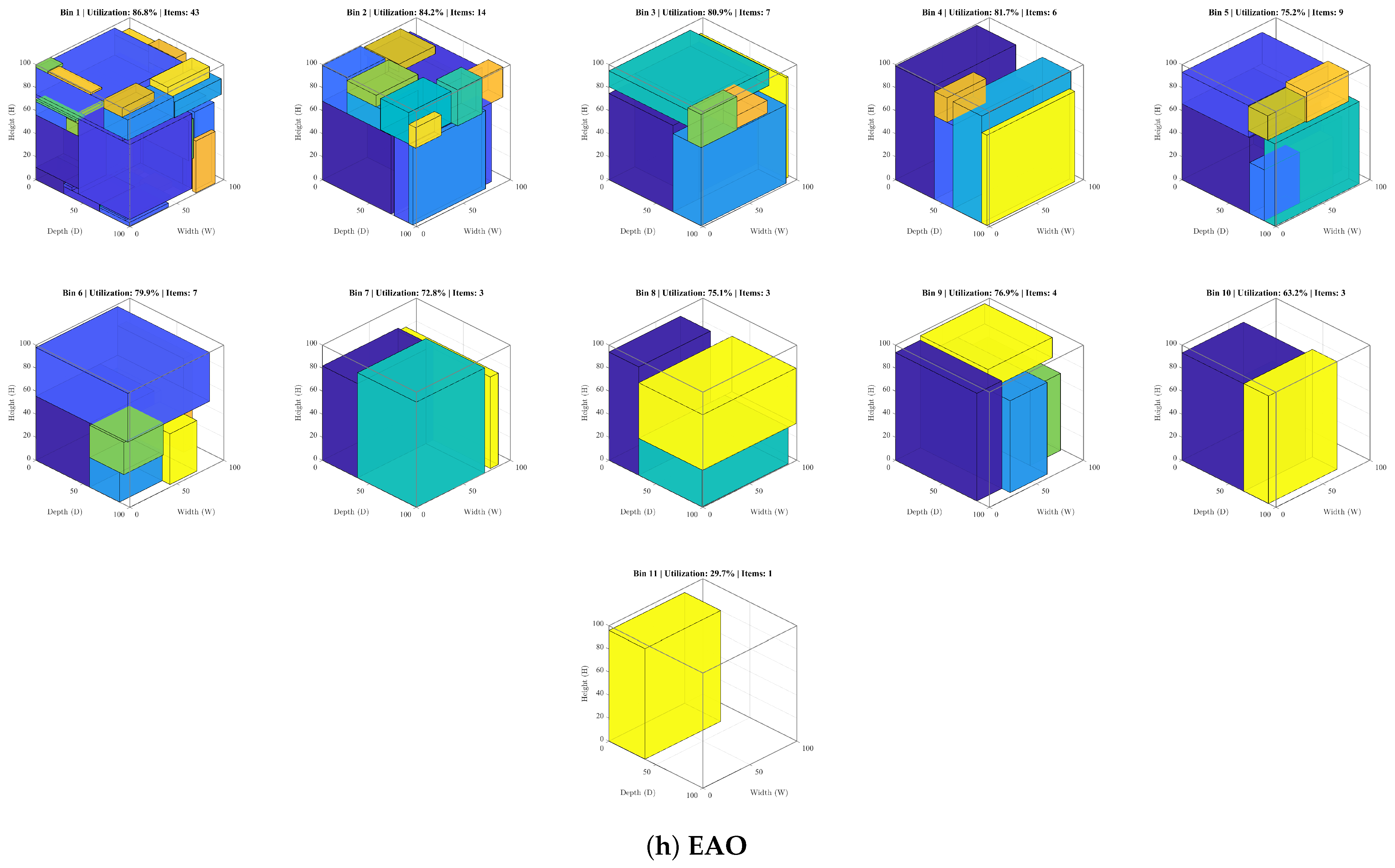
Figure 2. Overall architecture of the proposed HAGWO approach for 3D-BPP.
Mathematics 14 03011 g002
Figure 3. Visual representation of the DP (difference process). (a) The item awaiting placement alongside the initial maximal space. (b) The item positioned inside the maximal space. (c) The updated maximal spaces generated thereafter.
Mathematics 14 03011 g003
Figure 4. Illustration of the DFTRC-2 heuristic for packing box 2.
Mathematics 14 03011 g004
Figure 5. Qualitative visualization illustrating how the proposed HAGWO explores the search space on selected 30-dimensional CEC 2017 benchmark functions. The graphical representations include the 3D landscape, historical search traces, mean fitness evolution, trajectory along the first dimension, convergence behavior, and the interplay between exploration and exploitation.
Mathematics 14 03011 g005
Figure 6. Radar plots of HAGWO and other algorithms on the CEC2017 test suite (Dim = 30).
Mathematics 14 03011 g006
Figure 7. Friedman mean ranks for the CEC2017 benchmark suite at 50 and 100 dimensions.
Mathematics 14 03011 g007
Figure 8. Convergence curves of the best solution quality (measured by aNB) for Class 5 instances across the compared algorithms.
Mathematics 14 03011 g008
Table 1. Key parameter settings for each algorithm.
AlgorithmYearParameterValue
PSO [3]1995Inertia weight wLinearly decreasing from 0.9 to 0.4
Cognitive c 1 , Social c 2 2.0
GWO [10]2014Control parameter a 2 t · ( 2 / T max )
BSA [31]2013Mixrate1.0
Scaling factor F 3 · N ( 0 , 1 )
BRKGA [14]2011Elite fraction0.10
Mutant fraction0.15
Crossover probability ρ e 0.70
WOA [6]2016Control parameter a 2 2 · ( t / T max )
Spiral shape constant b1
CCO [18]2025Parameters a , b , C , T , w , d i e Default values from original paper
EAO [19]2025Initial catalytic rate k 0 0.1
HAGWOControl parameter a 2 2 · ( t / T m a x )
Dynamic weight p 1 t / T m a x
Levy flight parameter λ 1.5
Dynamic disturbance d f 0.1 × ( 1 t / T m a x ) × L e v y ( λ )
Superior wolf ratio (early/late) 0.1 × N / 0.3 × N
Medium wolf ratio (early/late) 0.3 × N / 0.3 × N
Inferior wolf ratio N n ς n ζ
Table 2. Results of the ablation study on the CEC 2017 benchmark suite at 30D (mean ± std over 30 independent runs; the best mean in each row is in bold). The symbols −/≈/+ indicate that the corresponding variant is significantly worse than, statistically comparable to, or significantly better than the full HAGWO according to the Wilcoxon signed-rank test at α = 0.05 .
Fun.GWOHAGWO–w/o-SHAGWO–w/o-AHAGWO–w/o-LHAGWO
F12.01E+09
(1.68E+09)
8.51E+08
(7.86E+08)
7.48E+08 
(4.77E+08)
1.18E+09
(1.04E+09)
1.08E+09
(1.20E+09)
F37.70E+04 +
(1.66E+04)
1.12E+05
(2.63E+04)
5.15E+04 +
(1.70E+04)
8.55E+04
(2.19E+04)
9.57E+04
(2.47E+04)
F46.27E+02
(8.35E+01)
5.90E+02
(5.70E+01)
5.57E+02
(4.12E+01)
5.74E+02
(4.40E+01)
5.55E+02
(4.57E+01)
F56.33E+02
(5.22E+01)
5.80E+02 
(2.25E+01)
6.30E+02
(6.42E+01)
5.84E+02
(2.11E+01)
5.83E+02
(2.01E+01)
F66.11E+02
(3.86E+00)
6.04E+02 
(3.09E+00)
6.06E+02
(2.79E+00)
6.05E+02
(2.80E+00)
6.05E+02
(1.61E+00)
F79.82E+02
(6.91E+01)
8.36E+02 
(3.35E+01)
9.29E+02
(6.20E+01)
8.66E+02
(3.10E+01)
8.48E+02
(4.48E+01)
F89.44E+02
(6.49E+01)
8.87E+02
(3.40E+01)
9.34E+02
(6.20E+01)
8.87E+02
(2.29E+01)
8.82E+02
(2.26E+01)
F94.36E+03
(2.20E+03)
2.03E+03 
(1.24E+03)
2.62E+03
(1.42E+03)
2.44E+03
(1.16E+03)
2.24E+03
(9.89E+02)
F106.35E+03
(2.02E+03)
4.58E+03 
(8.08E+02)
7.60E+03
(1.87E+03)
4.60E+03
(9.42E+02)
4.65E+03
(1.14E+03)
F112.35E+03
(1.53E+03)
1.53E+03
(2.99E+02)
1.36E+03 
(1.05E+02)
1.54E+03
(3.10E+02)
1.44E+03
(1.55E+02)
F121.51E+08
(1.18E+08)
6.96E+07
(6.74E+07)
8.33E+07
(1.12E+08)
6.54E+07
(6.17E+07)
6.29E+07
(5.70E+07)
F132.86E+07
(8.75E+07)
1.41E+06
(5.40E+06)
3.21E+05 +
(5.41E+05)
9.48E+06
(3.46E+07)
1.34E+06
(5.49E+06)
F148.89E+05
(1.12E+06)
3.26E+05
(4.05E+05)
2.30E+05 +
(3.03E+05)
4.04E+05
(5.53E+05)
4.60E+05
(5.09E+05)
F158.05E+05
(1.61E+06)
3.46E+05
(8.68E+05)
1.65E+05
(3.86E+05)
1.60E+05
(2.61E+05)
1.52E+05
(3.16E+05)
F162.84E+03
(4.31E+02)
2.58E+03
(2.09E+02)
2.67E+03
(4.83E+02)
2.53E+03
(2.54E+02)
2.50E+03
(3.23E+02)
F172.17E+03
(2.41E+02)
2.06E+03
(1.77E+02)
2.07E+03
(2.03E+02)
2.07E+03
(1.40E+02)
2.06E+03
(1.79E+02)
F183.70E+06
(6.14E+06)
2.52E+06
(3.07E+06)
1.73E+06
(1.71E+06)
1.75E+06
(1.98E+06)
1.32E+06
(1.43E+06)
F191.34E+06
(1.90E+06)
1.06E+06
(2.26E+06)
8.36E+05
(1.48E+06)
9.61E+05
(1.03E+06)
6.68E+05
(7.20E+05)
F202.56E+03
(2.22E+02)
2.43E+03 
(1.28E+02)
2.53E+03
(3.26E+02)
2.44E+03
(2.10E+02)
2.44E+03
(1.62E+02)
F212.43E+03
(5.45E+01)
2.38E+03
(2.99E+01)
2.42E+03
(5.48E+01)
2.39E+03
(1.90E+01)
2.38E+03
(1.76E+01)
F225.46E+03
(2.58E+03)
5.24E+03
(1.93E+03)
6.23E+03
(3.24E+03)
5.37E+03
(1.49E+03)
4.78E+03
(1.70E+03)
F232.81E+03
(5.85E+01)
2.74E+03
(2.67E+01)
2.78E+03
(6.99E+01)
2.75E+03
(3.18E+01)
2.74E+03
(3.02E+01)
F243.01E+03
(7.15E+01)
2.89E+03 
(2.30E+01)
2.98E+03
(7.37E+01)
2.92E+03
(3.34E+01)
2.89E+03
(1.84E+01)
F253.02E+03
(6.98E+01)
2.96E+03
(3.27E+01)
2.95E+03 
(2.26E+01)
2.97E+03
(2.87E+01)
2.98E+03
(5.57E+01)
F265.04E+03
(4.67E+02)
4.54E+03 
(3.83E+02)
4.84E+03
(5.75E+02)
4.62E+03
(4.98E+02)
4.67E+03
(2.60E+02)
F273.28E+03
(3.71E+01)
3.25E+03
(1.98E+01)
3.24E+03 
(1.45E+01)
3.26E+03
(2.35E+01)
3.25E+03
(2.05E+01)
F283.53E+03
(1.75E+02)
3.41E+03
(8.40E+01)
3.35E+03 +
(4.62E+01)
3.43E+03
(8.42E+01)
3.40E+03
(7.95E+01)
F293.98E+03
(2.19E+02)
3.88E+03
(1.84E+02)
3.86E+03
(2.90E+02)
3.84E+03
(1.95E+02)
3.84E+03
(1.28E+02)
F301.48E+07
(1.06E+07)
7.75E+06
(6.58E+06)
6.74E+06
(4.38E+06)
6.81E+06
(6.33E+06)
6.53E+06
(5.15E+06)
Friedman mean rank4.832.452.862.971.90
−/≈/+22/6/11/28/09/16/41/28/0
Table 3. Type characterization.
Type w j Interval h j Interval d j Interval
Type 1 [ 1 , 1 2 W ] [ 2 3 H , H ] [ 2 3 D , D ]
Type 2 [ 2 3 W , W ] [ 1 , 1 2 H ] [ 2 3 D , D ]
Type 3 [ 2 3 W , W ] [ 2 3 H , H ] [ 1 , 1 2 D ]
Type 4 [ 1 2 W , W ] [ 1 2 H , H ] [ 1 2 D , D ]
Type 5 [ 1 , 1 2 W ] [ 1 , 1 2 H ] [ 1 , 1 2 D ]
Table 4. Results for the three-dimensional instances (average over 10 runs). All algorithms were adapted to 3D-SBSBPP using the same biased random-key encoding, DFTRC-2 heuristic, and aNB fitness function.
ClassBin SizenBRKGAHAGWOGWOWOA
aNBNBaTaNBNBaTaNBNBaTaNBNBaT
1 100 × 100 × 100 5012.5612.2156.1512.5312.2148.6312.3612133.5412.5912.2141.06
10024.3123.9497.1224.2924482.5923.9523.6481.6924.5724.2508.77
2 100 × 100 × 100 5012.1511.8172.7412.0411.7159.5011.9411.5145.9012.0811.7154.97
10024.3324519.6224.3424524.0123.9023.6497.1424.4624.1536.95
3 100 × 100 × 100 5011.9111.5163.8911.8011.3149.1811.8011.4138.8312.0211.6146.29
10024.3624535.7824.2423.9528.1923.7223.3506.1524.5724.2529.94
4 100 × 100 × 100 5030.4030.2173.1730.4030.2153.1230.4030.2137.7130.4030.2143.43
10060.8860.7479.3660.8860.7471.0460.8860.7459.9960.8860.7460.71
5 100 × 100 × 100 507.687.3254.077.637.2251.467.617.2225.537.657.2225.99
10014.3413.9870.6014.1713.7953.4714.2713.9859.8214.4814.1868.25
6 10 × 10 × 10 5011.9711.697.5911.9011.689.6411.7511.481.0811.9911.687.52
10022.6122.3259.4922.1621.8246.1621.9721.6230.2222.6522.3247.40
7 40 × 40 × 40 506.996.7194.216.926.6190.666.906.6175.556.996.7184.87
10012.7412.4589.8512.4712.1572.0112.3311.9547.9612.8512.6604.31
8 100 × 100 × 100 509.479.1222.949.308.9194.799.318.9202.929.489.2108.2
10017.6017.3699.1517.1716.8639.9417.0016.6603.6517.6017.3645.04
Total2989296729442999
ClassBinSize n PSOBSACCOEAO
aNBNBaTaNBNBaTaNBNBaTaNBNBaT
1 100 × 100 × 100 5012.5912.3141.8612.6012.2148.5712.6512.3145.7312.7312.3148.55
10024.6624.3502.0324.6724.3505.0624.7924.4514.5824.9524.6518.62
2 100 × 100 × 100 5012.2111.9153.9012.2812160.8812.1611.8155.6712.3812161.44
10024.4624.1510.9824.4824.1536.2924.5124.1523.9324.7724.4550.28
3 100 × 100 × 100 5012.0111.6143.3011.9811.5152.7612.0511.6152.2712.2011.9154.09
10024.5424.2533.3824.5124.1547.4224.7224.4537.1624.7624.4553.37
4 100 × 100 × 100 5030.4030.2144.6430.4030.2142.4030.430.2140.7030.4030.2143.24
10060.8860.7456.9460.8860.7458.1260.8860.7450.3460.8860.7458.67
5 100 × 100 × 100 507.657.2251.417.727.3266.447.677.2253.007.857.4275.56
10014.4814.1880.1214.6214.3940.8114.5214.2910.4514.8314.5983.79
6 10 × 10 × 10 5011.9711.684.2012.1211.888.2212.1211.889.4912.2611.991.86
10022.5922.3245.8522.7822.4255.7922.7222.4246.3823.3223258.45
7 40 × 40 × 40 506.906.6178.697.046.7196.797.126.9192.737.247204.46
10012.7912.5597.2512.8812.6631.4012.9212.6617.2413.1412.8654.45
8 100 × 100 × 100 509.409.1195.479.589.3208.809.529.2199.209.739.4212.66
10017.4817.2670.6417.6717.4695.9517.7117.4675.6817.9717.6705.93
Total2999300930123041
Disclaimer/Publisher’s Note: The statements, opinions and data contained in all publications are solely those of the individual author(s) and contributor(s) and not of MDPI and/or the editor(s). MDPI and/or the editor(s) disclaim responsibility for any injury to people or property resulting from any ideas, methods, instructions or products referred to in the content.