New Methodology for Nonlinear EHD Interfacial Stability Between Two Electrified Viscoelastic Liquids

Abstract

This work examines a new methodology for the nonlinear electrohydrodynamic interfacial stability of dielectric viscoelastic liquids to enhance the predictive accuracy of microfluidic and biological applications. It tackles the intricacies of nonlinear coupled dynamics, encompassing interfacial deformation and viscoelastic stress influences. This study examines nonlinear stability, as linear stability has previously been thoroughly scrutinized. The interacting fluids are distinguished by differences in density, dielectric permittivity, permeability, viscoelastic parameters, surface tension, and their dynamic response at the perturbed interface. To simplify the mathematical organization, viscous potential flow theory is adopted. Further reduction is achieved by coupling linearized governing partial differential equations with the applicable nonlinear interfacial boundary conditions. This formulation leads to a nonlinear Mathieu oscillator, which governs the evolution of interface displacement. By adopting a non-perturbative approach, the achieved nonlinear ordinary differential equation is transformed into an equivalent linear one. Numerical solutions to the derived stability conditions reveal that the fundamental stability behavior remains qualitatively identical to both the real and complex coefficients associated with nonlinear characteristic equations describing the movement of interfacial displacement. The findings demonstrate that the Darcy number negatively influences the stability region, whereas kinematic viscosities, the Weber number, and Ohnesorge number facilitate the system’s stabilizing impact.

1. Introduction

EHD is extensively utilized across various sectors. The increasing necessity for comprehensive investigation into the fundamental EHD underlying its diverse real-world applications has been emphasized [1]. Numerous studies have examined the impact of an oblique EF on the formation of RTI at the boundary of a viscous, electrically conducting fluid layer of limited thickness in the presence of ST [2,3]. The findings indicate that the stability of the interface is acutely responsive to the strength and orientation of EF [3]. Mathematical models were developed to examine the interfacial stability of KHI under EHD effects [4]. A variety of geometric and physical provisions were analyzed to formulate stability requirements [5]. The Rivlin–Ericksen model was recognized as essential because of its relevance to real-world viscoelastic cylindrical liquids [6]. The instability of surface waves between two cylindrical viscoelastic fluids subjected to a tangential EF was analyzed. The MTSM produced two nonlinear Schrödinger PDEs of wave evolution. The design of pumps and switches for non-conductive electrolyte solutions, a notable subgroup of electro kinetic devices, represents progress [7]. A tendency of instability at the interface of two cylindrical fluids was identified [8]. The EHD instability at the interface of two viscous liquids within a tube exposed to a perpendicular EF was examined [9]. The evolution of electro-conductive motions in a low-conductivity liquid was observed using a horizontal capacitor [10]. The stability behavior of a dielectric viscous liquid caused by an EF was examined [11]. The methodological framework of the present study, employing nonlinear stability analysis through the NPA, represents a significant divergence from previous research and offers an innovative viewpoint on nonlinear EHD stability.

Viscoelastic liquids, which exhibit both viscosity and elasticity properties, are particularly significant due to their extensive applications in the production of food items [12]. The non-Newtonian Walters’ B model was employed to examine the stability of two second-order liquids characterized by elevated kinematic viscosity and viscoelasticity in the presence of a horizontal MF [13]. The system was shown to oscillate between stable/unstable regimes of continuously varying orderings depending on specific physical characteristics. Generalizations were particularly crucial in glass-forming processes and polymeric liquids, where the stress tensor must be regarded as an independent variable in hydrodynamic models [14]. To evaluate the influence of a vertical EF on a dielectric viscoelastic interface separating two streaming liquids exhibiting nonlinear stability behavior, the interfacial stability between two superimposed liquids was analytically and numerically analyzed [15]. Additionally, a cylindrical interface between two Walters’ B viscoelastic fluids within saturated porous media was identified [16]. Extensive research has focused on the Oldroyd-B model within porous media, owing to its importance in various disciplines, including geophysics, biology, chemistry, and oil recovery technologies [17]. A linear stability analysis of an electrified interface between two coaxial Oldroyd-B fluids was conducted [18]. Reports indicate EHD instability at a cylindrical interface, where two nonhomogeneous, permeable, incompressible dielectric liquids rotate at constant angular velocities around a shared axis [19]. The nonlinear stability of the cylindrical Walters’ B model was further validated because of its significance in various engineering and scientific applications [20]. A system of linked nonlinear PDEs characterizing unstable three-dimensional flows of a viscoelastic fluid, governed by a differential-type constitutive law, within a porous material was analyzed [21]. In the case of an incompressible medium, the equations describing velocity, pressure, and the stress tensor constitute a closed first-order system that include both real and complex components, thereby increasing the difficulty of establishing the corresponding initial boundary-value problem [22]. A study was conducted on the constant flow of a dilute polymer solution in water passing through a cylindrical pipe subjected to a longitudinal pressure gradient [23]. Moreover, the mixed boundary-value problem for steady incompressible motion in a Jeffrey-type viscoelastic medium confined to a fixed three-dimensional region was analyzed [24]. In addition, the boundary-control problem for the Darcy–Brinkman–Jeffrey system, representing steady flows of incompressible viscoelastic fluids in 2D and 3D porous media, was explored [25].

The growth rate of EHD instability in a Maxwell fluid, devoid of inertia, becomes unbounded beyond a critical Deborah number [26]. A hypothesis explaining the electro-viscoelastic behavior of liquid–liquid interfaces was developed [27]. Theoretical analysis was performed to assess the interfacial stability between two horizontally stratified viscous fluids, one conductive and the other non-conductive, under the action of a vertically oscillating EF [7]. Damped oscillators exhibit a greater association with physical reality than their undamped counterparts, which depend solely on theoretical formulations [28]. This discovery has prompted ongoing research to enhance analytical and NS theoretical and computational methods employed in investigating higher-order nonlinearities in damped oscillators [29]. The HFF and its improved variations were compared with residual computations [30]. Several improved residual-based approaches exist for accurately determining the frequency of nonlinear oscillators. The residuals associated with two approximate solutions were meticulously examined using the fundamental concept of HFF [31]. The efficacy of the method was shown through the application of severely nonlinear oscillators. It was highlighted that a straightforward and effective strategy for nonlinear oscillators could achieve sufficient accuracy in frequency prediction [32]. The HFF was effectively incorporated into an undamped oscillator and its various extensions [33]. Simultaneously, significant research has focused on the nonlinear stability of fully saturated two-fluid systems in porous media, where the interplay between permeability, viscosity contrast, and interfacial forces results in intricate stability behavior [34,35].

Although several recent studies have investigated nonlinear instability phenomena under periodic electromagnetic forcing [36,37,38], the present work differs in both physical formulation and analytical treatment. Ref. [36] examined nonlinear interfacial instability between Walters’ B/Rivlin–Ericksen fluids under periodic EFs, whereas the current study develops a generalized electrohydrodynamic formulation for dielectric viscoelastic liquids based on viscous potential flow theory and a nonlinear Mathieu-oscillator framework. Moreover, Refs. [37,38] focused on magnetically induced instability mechanisms in fluid jets and Bingham-fluid interfaces, respectively, while the present investigation considers electrically driven instability in porous media and examines the coupled effects of electric forcing, viscoelasticity, permeability, viscosity, and ST on both the temporal response and stability characteristics of the interface. These features constitute the primary novelty and contribution of the present work.

A new approach in examining the nonlinear EHD stability of a pair of electrified viscoelastic liquids subjected to normal periodic EFs is of great importance in a variety of contemporary technological applications. The methodology facilitates the optimization of energy-efficient EHD pumping and actuation systems, in addition to the development of smart materials and adaptive surfaces that utilize periodic EFs to dynamically adjust interfacial morphology. In summary, investigating nonlinear EHD stability under normal periodic EFs connects feasibility with commercial relevance, facilitating the resilient design and regulation of advanced EHD systems that incorporate intricate viscoelastic fluids. The paper’s structure is organized as follows. The mathematical foundation of the EHD problem and a summary of the key governing PDEs of motion are presented in Section 2. The nonlinear characteristic equation is derived in Section 3. The polar representation of the characteristic ODE is presented in Section 4. The generalized approach for identifying nonlinear surface waves is given in Section 5, highlighting a number of important aspects of the phenomena. Lastly, Section 6 provides a summary of the study’s key findings.

2. Mathematical Modeling

In this study, fluid motion is analyzed in the vicinity of a planar interface. It is presumed that there is no MHT between the two fluids. Furthermore, the two fluids flow with two distinct uniform velocities. Consequently, the physical model follows KHI. Our research is limited to tiny viscoelastic effects due to the intrinsic complexity of the dynamics of non-Newtonian dielectric liquids with shifting boundaries. The perturbation technique is used to concentrate the analysis on viscoelastic effects within the framework of VPT since the bulk flow away from the interface can be reasonably represented as an irrotational fluid. Only in a thin vertical interfacial layer are these effects anticipated to be substantial. To account for viscoelastic effects, a unique method is used to incorporate a normal-direction damping stress into BCs. In accordance with VPT [39,40,41,42], which assumes that the overall damping stress work rate equals the total rate of mechanical energy dissipation, an analogous topic is previously investigated using classical perturbation theory. Derivatives are only taken within the VPT framework in order to avoid the laborious manipulation of the complete weak-fluid equations. It is simple to make changes to the interfacial BCs, where the minor viscoelastic effects arise, as the governing PDEs for an irrotational flow reduce to Laplace’s equation. These viscoelastic contributions are directly defined inside the usual stress BCs in the existing analysis. The majority of liquid phases are branded as homogeneous, incompressible, dielectric materials under the viscoelastic assumption. It is assumed that the two liquids’ interface is flat and well defined. The following is an expression of the fundamental relationships that describe the liquids’ viscoelastic behavior [6]:

$${\sigma }_{ij}^{hydro}=-P_j{\delta }_{ij}+\left[{\mu }_j+{\nu }_j\left({\displaystyle \frac{\partial }{\partial t}}+V_k{\displaystyle \frac{\partial }{\partial x_k}}\right)\right]\left({\displaystyle \frac{\partial V_i}{\partial x_j}}+{\displaystyle \frac{\partial V_j}{\partial x_i}}\right),$$

(1)

where $\underset{¯}{V}$ is the liquid velocity, ${\delta }_{ij}$ denotes the Kronecker delta, and ${\sigma }_{ij}^{hydro}$ is the hydrodynamic stress tensor. Additionally, $P_j$ stands for hydrostatic pressure, ${\mu }_j$ for the viscosity coefficient, and ${\nu }_j$ for the viscoelastic parameters.

Viscoelasticity refers to the characteristics of materials that display both viscous and elastic responses when deformed, crucial to the inspection of complex fluids, polymers, and biological tissues. In hydrodynamic stress, the viscous component signifies immediate resistance to deformation; concurrently, viscoelastic materials can produce supplementary stresses attributable to deformation rates and their historical responses. This facilitates energy storage and release, resulting in phenomena such as stress relaxation, creep, hysteresis, and normal stress differentials. The precise modeling of viscoelastic materials necessitates sophisticated constitutive equations that incorporate supplementary stress tensors and relaxation durations to accurately characterize delayed flow responses.

The stress tensor shown in Equation (1) signifies the hydrodynamic stress tensor in a viscous time-dependent fluid. It involves two of the foremost portions: an isotropic pressure effect and viscous stress influence. The term $-P_j{\delta }_{ij}$ designates normal stress caused by fluid pressure, substituting correspondingly into all guidelines and encouraging fluid compression. The second term captures viscous effects and depends on the fluid’s dynamic viscosity ${\mu }_j$ and an additional coefficient ${\nu }_j$, along with the rate of the deformation tensor ${\displaystyle \frac{\partial V_i}{\partial x_j}}+{\displaystyle \frac{\partial V_j}{\partial x_i}}$, which measures how the fluid elements stretch and shear. The operator ${\displaystyle \frac{\partial }{\partial t}}+V_k{\displaystyle \frac{\partial }{\partial x_k}}$ represents the material or convective derivative, indicating that the viscous stresses arise from both time and fluid motion. 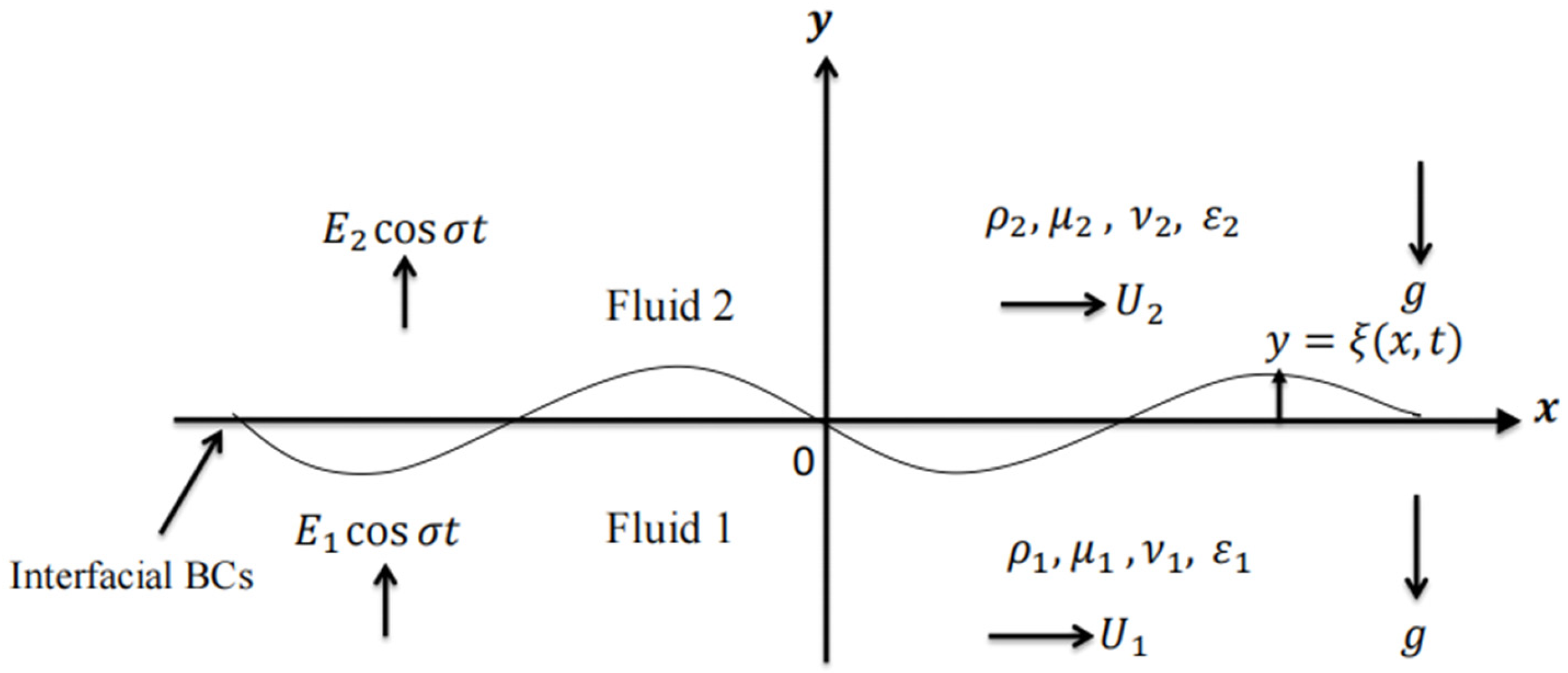Altogether, this formulation describes how internal stresses arise from the pressure and velocity gradient, governing momentum transport and deformation in complex fluid flows (Figure 1).

The model incorporates gravitational influences as crucial elements. The analysis is restricted to a two-dimensional Cartesian framework; for simplicity’s sake, system $(x, y)$ along the $y-$ axis is aligned as normal to the interface. For the bottom and higher fluids, respectively, the liquid densities are represented by ${\rho }_1$ and ${\rho }_2$ and their dielectric constants by ${\epsilon }_1$ and ${\epsilon }_2$. The bottom and top fluid layers are always identified by the indices 1 and 2. Suitably, the permeability of the two phases is assumed to be the same, represented by parameter $\alpha$, and the porosity of both liquids is considered to equal unity. The fluids have constant velocities $U_1$ and $U_2$ and flow in the positive $x-$ direction. A periodic EF that acts across the medium is also applied to the system. The analysis disregards the existence of free surface charges at the interface and assumes that no volumetric charges are present within either of the liquid phases. Under these assumptions, the interfacial electric forces are represented through the Maxwell stress tensor, given by [2,3]

$${\sigma }_{ij}^{elec}={\epsilon }_j{E}_i{E}_j-{\displaystyle \frac{1}{2}}{\epsilon }_j{E}^2{\delta }_{ij}.$$

(2)

The following is a consistent way to represent the total operational stress tensor [4]:

$${\sigma }_{ij}={\sigma }_{ij}^{hydro}+{\sigma }_{ij}^{elec}.$$

(3)

Therefore, the following is the formulation of a periodic EF acting on the interface:

$${\underset{¯}{E}}_j=E_j\cos \sigma t{\underset{¯}{e}}_y, j=1,2,$$

(4)

where the unit vector along the $y-$ axis is denoted by ${\underset{¯}{e}}_y$

$${\rho }_j\left[{\displaystyle \frac{\partial {\underset{¯}{V}}_j}{\partial t}}+({\underset{¯}{V}}_j.\nabla ){\underset{¯}{V}}_j\right]=-\nabla P_j-{\rho }_j\underset{¯}{g}{\underset{¯}{e}}_y-{\displaystyle \frac{{\mu }_j}{\alpha }}{\underset{¯}{V}}_j, j=1,2$$

(5)

where ${\underset{¯}{V}}_j={\underset{¯}{V}}_j(x,y;t)$ is the velocity field of the liquid phase, and $P_j$ is the related hydrostatic pressure.

The constraint of incompressibility may be written as

$$\nabla .{\underset{¯}{V}}_j=0.$$

(6)

Given this factor, the interface displacement can be written as follows [43]:

$$y=\xi \left(x;t\right).$$

(7)

The deflection function $\xi (x;t)$ describes the rise or deviation in the interface from its equilibrium configuration. It is common practice in the context of interfacial stability studies to assume that the interface perturbation is a spatially harmonic one; this enables the disturbance to be expressed as a time-varying sinusoidal wave:

$$\xi (x,t)=\eta (t)\cos kx.$$

(8)

The representation $\xi (x;t)=\eta (t)\cos kx$ corresponds to a single-mode truncation of interface dynamics. This is equivalent to a Galerkin-type projection onto the fundamental mode, assuming that higher harmonics generated by nonlinear interactions remain small. The obtained ODE should be interpreted as an approximate reduced model, valid for moderate disturbance amplitudes.

Additionally, it is expected that this function satisfies the Dirichlet BC listed below:

$$\xi (0,t)=\eta (t),$$

(9)

where there are two ICs of the function $\eta (t)$. These ICs may be written as follows:

$$\eta (0)=A\mathrm{and} \dot{\eta }(0)=0,$$

(10)

where $A$ represents the amplitude of the initial disturbance.

The growth in interfacial disturbance is expressed using the normal mode formulation given below:

$$\xi (x,t)=\eta (t)e^{ikx}+c.c.,$$

(11)

where $c.c.$ stands for the preceding^’ complex conjugate.

The interface is described by the following expression [43,44]:

$$S(x,y;t)=y-\xi (x;t).$$

(12)

Consequently, the outward unit normal to the interface is given by [43,44]

$$\underset{¯}{n}={\displaystyle \frac{\nabla S}{\left|\nabla S\right|}}=\left(-{\xi }_x{\underset{¯}{e}}_x+{\underset{¯}{e}}_y\right){\left(1+{\xi }_x^2\right)}^{-1/2},$$

(13)

with ${\underset{¯}{e}}_x$ and ${\underset{¯}{e}}_y$ representing the unit vectors in the $x-$ and $y-$ directions, respectively.

The following statement is produced by the pure balance’s zero-order pressure as [43,44]

$$P_{0j}=-{\rho }_{j}gy-{\displaystyle \frac{{\mu }_j}{\alpha }}{U}_{j}x+C_{0j},$$

(14)

with the integration constants represented by $C_{0j}$.

The zero-order contribution of the normal stress tensor at the displaced contact produces the following expression:

$$C_{o1}-C_{02}={\displaystyle \frac{1}{2}}\left({\epsilon }_1{E}_1^2-{\epsilon }_2{E}_2^2\right){\cos }^2\sigma t-gy\left({\rho }_1-{\rho }_2\right)-{\displaystyle \frac{x}{\alpha }}\left({\mu }_1{U}_1-{\mu }_2{U}_2\right).$$

(15)

The Navier–Stokes equations can be simplified to Euler equations when formulated within the framework of VPF, as was previously discussed [39,40,41,42]. Consequently, the exclusion of the liquid’s viscous stress tensor from the momentum balance is incorporated into the basic structural formulation at the inlet. The obtained equation describes the flow behavior of an incompressible viscous fluid through a porous medium, in agreement with the Brinkman–Darcy modified formulation. The fluid is treated as irrotational in accordance with the basic concepts of VPT. Furthermore, finite-amplitude two-dimensional perturbations are imposed on both the linear governing PDEs and the BCs to investigate the interfacial stability of the system. It is discovered that the flow shows dependence on both the horizontal and vertical axes of propagation when such a two-dimensional finite perturbation is considered; consequently, the overall velocity field can be written as

$${\underset{¯}{V}}_j={\mathrm{U}}_j{\underset{¯}{e}}_x+\nabla {\varphi }_j={\displaystyle \frac{\partial {\varphi }_j}{\partial y}}{\underset{¯}{e}}_y+\left({\mathrm{U}}_j+ik{\varphi }_j\right){\underset{¯}{e}}_x,$$

(16)

This arises from the incompressibility constraint and must align with the Laplace formulation:

$${\nabla }^2{\varphi }_j=0.$$

(17)

The governing PDEs of motion, the continuity equation, and the BCs are examined in a two-dimensional framework, with a slight perturbation applied to the system in order to assess the interfacial stability of the current situation. A small departure from the initial structure is anticipated for two-dimensional flow. The different disturbances can be described as follows under these assumptions:

$$F(x,y;t)=\hat{f}(y,t)e^{ikx}+c.c.,$$

(18)

where $F(x,y;t)$ stands for any perturbed quantity.

As previously shown [43,44], the velocity potentials can therefore be represented using Equation (17):

$${\varphi }_1(x,y;t)=A_1(t)e^{k\left(ix+y\right)}, -\infty \le y\le \xi ,$$

(19)

and

$${\varphi }_2(x,y;t)=A_2(t)e^{k\left(ix-y\right)}, \xi \le y\le \infty ,$$

(20)

where the proper nonlinear BCs will be used to calculate the time-dependent functions $A_1(t)$ and $A_2(t)$.

The nonlinear evolution process and the linear approximation are combined to apply the interfacial stability framework. Accordingly, the perturbed pressure $P_j$ can be derived from Equation (5) as follows:

$$P_j=-{\rho }_j\left({\displaystyle \frac{\partial {\varphi }_j}{\partial t}}+ik{U}_j{\varphi }_j\right)-{\displaystyle \frac{{\mu }_j}{\alpha }}{\varphi }_j.$$

(21)

When analyzing the system’s EHD behavior, a quasi-static approximation is used for simplicity. This assumption imposes the absence of free charges and allows for the disregard of external MFs. Similarly, magnetostatic effects are ignored [2]. Consequently, a scalar electric potential function can be used to determine the EF. The static form of Maxwell’s equation simplifies to Laplace’s equation because of the dielectric nature of the liquids. The disturbed EF under these circumstances can be written as

$${\underset{¯}{E}}_j=E_j\cos \sigma t {\underset{¯}{e}}_y-\nabla {\psi }_j.$$

(22)

Gauss’s law implies that Laplace’s equation must be satisfied by the scalar electric potential:

$${\nabla }^2{\psi }_j=0.$$

(23)

Therefore, ${\psi }_1(x,y;t)$ and ${\psi }_2(x,y;t)$ can be written as follows [43,44]:

$${\psi }_1(x,y;t)=B_1(t)e^{k\left(ix+y\right)}, -\infty \le y\le \xi ,$$

(24)

and

$${\psi }_2(x,y;t)=B_2(t)e^{k\left(ix-y\right)}, \xi \le y\le \infty ,$$

(25)

where two unknown time-dependent functions, $B_1(t)$ and $B_2(t)$, will be determined via the applicable BCs.

Nonlinear BCs

The treatment of BCs, especially the kinematic condition, necessitates additional elucidation. The manuscript must clearly articulate the assumptions underpinning the kinematic BC, present a precise derivation of its mathematical formulation, and elucidate its implementation within the suggested framework. A description of its compatibility with the governing PDEs and its impact on solution stability and correctness would enhance the rigor and transparency of the analysis. Since the normal stress tensor includes contributions from both the hydrodynamic and electric stress tensors, determining it is crucial. Accordingly, the interfacial disturbance at the perturbed contact needs to meet the corresponding nonlinear BCs. These BCs may be formulated as follows:

• The kinematic BC is given as

$${\xi }_t+\left(U_j+ik{\varphi }_j\right){\xi }_x={\displaystyle \frac{\partial {\varphi }_j}{\partial y}}, \mathrm{at} y=\xi . j=1, 2$$

(26)

• The potentials defined in Equations (24) and (25) must meet the following BCs at the separating interface:

The BCs for the EF in the EHD formulation necessitate a more rigorous analysis. The work must explicitly delineate the enforcement of the tangential and normal components of the EF at the interface, including the continuity of the tangential EF and the relevant jump BC for the normal component related to surface charge density and permittivity variations. An in-depth examination of these BCs and their application is crucial to guarantee the physical consistency and precision of the EHD model. It is assumed that no bulk electric charges exist in either liquid phase and that the interface is free of surface charges in its equilibrium state. Consequently, the tangential components of the EF and the normal component of electric displacement must remain continuous across the interface. As a consequence, the following relationships are obtained:

$$\underset{¯}{n}\wedge {\underset{¯}{E}}_1=\underset{¯}{n}\wedge {\underset{¯}{E}}_2, \mathrm{at} y=\xi .$$

(27)

Additionally, the regularity of the electric induction’s normal component results in

$$\underset{¯}{n}.\left({\epsilon }_1{\underset{¯}{E}}_1-{\epsilon }_2{\underset{¯}{E}}_2\right)=0, \mathrm{at} y=\xi .$$

(28)

The current model must solve the charge conservation equation in conjunction with the electrostatic and hydrodynamic equations together with suitable interfacial BCs for the surface charge density. The current study deliberately overlooks these effects as our aim is to examine the impact of the applied EF on the hydrodynamic stability of the interface within the ideal dielectric framework. This hypothesis is valid when the electrical conductivity of both liquids is adequately low, ensuring that the charge-relaxation duration significantly exceeds the typical time frame of the instability, or conversely, when conduction currents are insignificant relative to displacement currents. In these circumstances, the interface is essentially devoid of a surface charge and the established BCs are physically coherent. To eliminate any uncertainty, we have amended the paper to clearly indicate that the analysis is confined to the perfect dielectric approximation, wherein charge-accumulation and charge-relaxation phenomena are disregarded. We have also specified that expanding the analysis to encompass the leaky dielectric model, which incorporates interfacial charge dynamics, exceeds the boundaries of the current study and is a compelling avenue for further investigation.

3. Nonlinear Characteristic Equation

The stability of the current issue is examined by using the stress tensor normal component, which is predicted to be discontinuous by the presence of ST. The following is an expression of this BC [43,44]:

$$\underset{¯}{n}.\left({\underset{¯}{F}}_1-{\underset{¯}{F}}_2\right)=T\nabla .\underset{¯}{n}, \mathrm{at}y=\xi ,$$

(29)

where $\underset{¯}{F}$ stands for the generalized interfacial force, which has the following formal definition:

$$\underset{¯}{F}=\left(\begin{array}{cc}{\sigma }_{xx}& {\sigma }_{xy}\\ {\sigma }_{yx}& {\sigma }_{yy}\end{array}\right)\left(\begin{array}{c}{n}_x\\ n_y\end{array}\right),$$

(30)

where ${\sigma }_{ij}$ indicates the components of vector $\underset{¯}{n}$ and the total stress tensor $n_x$, $n_y$ are the elements of the unit normal vector $\nabla .\underset{¯}{n}$, and ${\sigma }_{ij}$ is the total stress tensor.

Furthermore, the following relationship provides an explicit expression for the divergence associated with the normal vector $\nabla .\underset{¯}{n}$ [4,16,20]:

$$\nabla .\underset{¯}{n}=-{\xi }_{xx}\left(1-{\displaystyle \frac{3}{2}}{\xi }_x^2\right).$$

(31)

The inclusion of Equations (19), (20), (24) and (25) into Equation (29) give the following specific solutions:

$${\varphi }_1={\displaystyle \frac{ \left({\xi }_t+U_1{\xi }_z\right)}{k\left(1-i{\xi }_x\right)}}{e}^{k\left(y-\xi \right)}, -\infty \le y\le \xi ,$$

(32)

$${\varphi }_2=-{\displaystyle \frac{ \left({\xi }_t+U_2{\xi }_z\right)}{k\left(1+i{\xi }_x\right)}}{e}^{k\left(\xi -y\right)}, \xi \le y\le \infty ,$$

(33)

$${\psi }_1={\displaystyle \frac{{\xi }_x e^{k\left(y-\xi \right)}}{k\left(1-i{\xi }_x\right)\left({\epsilon }_2+{\epsilon }_1\right)}}\left[i {\epsilon }_2 \left(E_2-E_1\right)\cos \sigma t\right], -\infty \le y\le \xi ,$$

(34)

and

$${\psi }_2={\displaystyle \frac{{\xi }_x e^{k\left(\xi -y\right)}}{k\left(1+i{\xi }_x\right)\left({\epsilon }_2+{\epsilon }_1\right)}}\left[i {\epsilon }_1 \left(E_1-E_2\right)\cos \sigma t\right]. \xi \le y\le \infty .$$

(35)

It should be noted that the denominators in Equations (32)–(35) are non-zero quantities. It is crucial to highlight that the denominators present in Equations (32)–(35) are unequivocally non-zero given the specified physical and mathematical premises. Consequently, these formulations are consistently defined and produce finite values for both the flow potentials as well as the EF, thus guaranteeing the regularity of the derived solutions. Consequently, these equations do not give rise to any mathematical singularity. The corresponding hydrodynamic pressures are thus obtained by putting Equations (32) and (33) into Equation (21):

$$P_1(x,y;t)=-{\rho }_{1}gy-{\displaystyle \frac{1}{k\left(1-i{\xi }_x\right)}}\left({\rho }_1\left({\xi }_{tt}+U_1{\xi }_{xt}+ik{U_1}^2{\xi }_x+ik{U}_1{\xi }_t\right) +{\displaystyle \frac{{\mu }_1}{\alpha }}\left({\xi }_t+U_1{\xi }_x\right)\right)e^{k\left(y-\xi \right)}, -\infty \le y\le \xi ,$$

(36)

and

$$P_2(x,y;t)=-{\rho }_{2}gy+{\displaystyle \frac{1}{k\left(1+i{\xi }_x\right)}}\left({\rho }_2\left({\xi }_{tt}+U_2{\xi }_{xt}+ik{U_2}^2{\xi }_x+ik{U}_2{\xi }_t\right) +{\displaystyle \frac{{\mu }_2}{\alpha }}\left({\xi }_t+U_2{\xi }_x\right)\right)e^{k\left(\xi -y\right)}, \xi \le y\le \infty .$$

(37)

Since our goal is to study temporal instability, the disturbance surface could be described as below in order to turn the PDEs into ODEs.

The application of non-dimensional analysis is imperative in the fields of fluid mechanics as well as dynamical systems. Now, a wave-fixed reference frame is considered. To put it another way, an observer is standing at $x=0$ after differentiating the surface displacement with regard to the $x-$ coordinate. The resulting characteristic equation can therefore be expressed in a non-dimensional form. This is accomplished by introducing a characteristic length $L$ and defining the relevant non-dimensional variables as follows:

Weber number $W_e={\rho }_1{U}_1^{2}L/T$, Bond number $B_n={\rho }_1 g L^2/T$, Darcy number $D_a=\alpha /L^2$, Ohnesorge number $Z={\mu }_1/\sqrt{{\rho }_1 T L}$, ${\xi }^{*}=\xi /L$, viscoelasticity number $W_B={\nu }_1/{\rho }_1{L}^2$, time $t^{*}=\sqrt{T/{\rho }_1 L^3}t$, ratio of liquid densities ${\rho }^{*}={\rho }_2/{\rho }_1$, ratio of dielectric constants ${\epsilon }^{*}={\epsilon }_2/{\epsilon }_1$, ratio of uniform velocities $U^{*}=U_2/U_1$, ratio of kinematic viscosities ${\mu }^{*}={\mu }_2/{\mu }_1$, and electric bond $E^{*2}=L {\epsilon }_1 E^2/T$. Consequently, for the sake of simplicity in the current analysis, the asterisk notation has been removed. To enhance convenience, a physical elucidation of these non-dimensional values can be summarized as follows:

Weber number: Signifies the rivalry between fluid inertia and ST. A high number signifies that inertial forces prevail, making the interface more prone to deformation, whereas a low value suggests that surface tension ensures a smoother and more stable interface.

Electric Bond number: Indicates the significance of electric forces in relation to ST. Greater values suggest that the exerted EF exerts a more significant impact on interface distortion and wave transmission, whereas lesser values show that capillary forces prevail.

Darcy number: Assesses the permeability of the porous material. A greater value signifies a medium with high permeability that presents minimal opposition to fluid movement, whereas a lesser value denotes a medium with reduced permeability that exerts greater resistance to flow.

Ohnesorge number: Indicates the impact of viscous dissipation in comparison to inertial and capillary forces. Elevated values signify enhanced viscous damping and the increased attenuation of interfacial waves, whereas diminished values reflect lesser viscous influences.

Viscoelasticity number: Measures the significance of elastic characteristics stemming from the fluid’s memory. Higher values suggest that elastic stresses considerably influence the flow and wave dynamics, whereas lower values relate to behavior more like that of a Newtonian fluid.

Comparison of liquid densities: Evaluates the density of the two fluid strata. This parameter regulates the allocation of inertia and buoyancy among the fluids and significantly affects wave propagation, interfacial stability, and the system’s dynamic response.

Ratio of dielectric constants: Evaluates the electrical polarizability between the two liquids. It dictates the distribution of the EF at the interface and affects the intensity of the electric stresses exerted on the fluid interface.

Ratio of consistent velocities: Evaluates the average velocities of the two fluid strata. It assesses the magnitude of velocity shear at the boundary, with greater disparities typically fostering more pronounced interfacial disruptions and heightening the probability of shear-induced instability.

Ratio of kinematic viscosities: Evaluates the rates of momentum diffusion between the two fluids. It regulates the comparative degrees of viscous dissipation inside each stratum and impacts the momentum transfer at the boundary, thereby affecting wave attenuation and flow stability.

To obtain the characteristic equation that determines the stability of the system, the basic governing PDEs of the perturbed motion are first linearized to an equilibrium state. Subsequently, a normal mode analysis is employed by assuming that all perturbation quantities vary, expressed as exponentially varying waves with respect to the horizontal coordinates and time. This assumption reduces the linearized PDE to an ODE for the disturbance amplitudes. The resulted PDE may be written as follows:

$$\begin{array}{c}{\xi }_{tt}+(a_1+i{b}_1){\xi }_t+(a_2+i{b}_2+d_1{\cos }^2\sigma t)\xi +c_1\xi {\xi }_{tt}+(a_3+i{b}_3)\xi {\xi }_t+(a_4+i{b}_4-d_2{\cos }^2\sigma t){\xi }^2\hfill \\ +c_2{\xi }^2{\xi }_{tt.}+(a_5+i{b}_5){\xi }^2{\xi }_t+(a_6+i{b}_6+d_3{\cos }^2\sigma t){\xi }^3=0\hfill \end{array}.$$

(38)

In order to enhance the main text’s readability and flow, the parameters $a_j,b_j,c_j and d_j$ are moved to Appendix A.

4. Polar-Form Representation

To better describe the oscillations and phase relationships, the complex coefficients are recast in polar representation. This approach simplifies the analysis by expressing the coefficients through amplitude–phase decomposition [44]. Therefore, the nonlinear PDE, as given in Equation (38), may be formulated as follows:

$$\begin{array}{c}{\xi }_{tt}+r_1{e}^{i{\theta }_1}{\xi }_t+(r_2{e}^{i{\theta }_2}+d_1{\cos }^2\sigma t)\xi +c_1\xi {\xi }_{tt}+r_3{e}^{i{\theta }_3}\xi {\xi }_t+(r_4{e}^{i{\theta }_4}-d_2{\cos }^2\sigma t){\xi }^2\hfill \\ +c_2{\xi }^2{\xi }_{tt}+r_5{e}^{i{\theta }_5}{\xi }^2{\xi }_t+(r_6{e}^{i{\theta }_6,}+d_3{\cos }^2\sigma t){\xi }^3=0\hfill \end{array},$$

(39)

where

$$r_j=\sqrt{a_j^2+b_j^2} \mathrm{and} {\theta }_j={\tan }^{-1}\left({\displaystyle \frac{b_j}{a_j}}\right) .$$

(40)

The real components of the coefficients remain; meanwhile, the imaginary components canceled each other when the complex conjugate of Equation (39) is incorporated into this equation. This style simplifies the equation’s structure and ensures that all generated coefficients are real, facilitating further comprehension and resolution:

$$\begin{array}{l}{\xi }_{tt}+r_1\cos {\theta }_1{\xi }_t+(r_2\cos {\theta }_2+d_1{\cos }^2\sigma t)\xi +c_1\xi {\xi }_{tt}+r_3\cos {\theta }_3\xi {\xi }_t+(r_4\cos {\theta }_4-d_2{\cos }^2\sigma t){\xi }^2\hfill \\ +c_2{\xi }^2{\xi }_{tt.}+r_5\cos {\theta }_5{\xi }^2{\xi }_t+(r_6\cos {\theta }_6+d_3{\cos }^2\sigma t){\xi }^3=0 \hfill \end{array}.$$

(41)

In accordance with the conventions of linear stability theory, each physical quantity is paired with its complex conjugate. For example, Equation (11) demonstrates the interfacial displacement in its complex form, whereas its associated physical (real) description is provided in Equation (12). In our earlier work, the nonlinear characteristic Equation (38) was examined in two consecutive phases. Initially, we examined a particular scenario, where the imaginary component disappeared owing to the lack of the Weber number. Accordingly, the characteristic equation is simplified to a polynomial with entirely real coefficients, facilitating the formulation of theoretical stability conditions. In the subsequent phase, the entire formulation, encompassing the Weber number, was analyzed. In this instance, the characteristic equation contained complex coefficients, rendering the analytical approach significantly more challenging. Due to the intricacy of the resultant nonlinear equation, a universal theoretical criterion could not be formulated, necessitating that the stability assessment depends solely on numerical calculations.

In the current study, we utilize the complex conjugate framework of the governing equations to reconfigure the characteristic equation. The nonlinear characteristic Equation (38) is converted into its corresponding real-form equation, shown in Equation (41), by merging the characteristic equation with its complex conjugate. This rephrasing removes the presence of intricate coefficients while maintaining the full dynamics of the initial issue. It is crucial to highlight that Equation (41) does not overlook the imaginary component; instead, it integrates both the real and imaginary parts of the original characteristic equation into a cohesive real-coefficient framework. As a result, the modified equation preserves all the physical data present in Equation (38) while offering a more advantageous structure for theoretical exploration and numerical application.

Conversion of PDE into an ODE

The PDE, as displayed in Equation (41), can be converted into an equivalent ODE by using the BC provided in Equation (10). This BC simplifies the equation by reducing it to derivatives relating to a single independent variable, effectively eliminating partial derivatives involving multiple variables from the final form:

$$\begin{array}{c}\ddot{\eta }+r_1\cos {\theta }_1\dot{\eta }+(r_2\cos {\theta }_2+d_1{\cos }^2\sigma t)\eta +c_1\eta \ddot{\eta }+r_3\cos {\theta }_3\eta \dot{\eta }+(r_4\cos {\theta }_4-d_2{\cos }^2\sigma t){\eta }^2\hfill \\ +c_2{\eta }^2\ddot{\eta }+r_5\cos {\theta }_5{\eta }^2\dot{\eta }+(r_6\cos {\theta }_6+d_3{\cos }^2\sigma t){\eta }^3=0 \hfill \end{array}.$$

(42)

The basic principles of the NPA for analyzing nonlinear dynamical systems are briefly described. The NPA allows nonlinear ODE to be transformed into linearized forms while retaining the core dynamic features of the governing system [45,46]. The obtained linear oscillator system accurately reproduces the temporal oscillatory response of the nonlinear system, providing an effective framework for analyzing nonlinear behavior with minimal deviation from the exact solution. Within this framework, the nonlinear system is reformulated as an equivalent system incorporating damping effects, under periodic excitation, considering nonlinear stiffness and damping effects that alter the natural frequency. Previously, El-Dib [46,47] demonstrated the applicability of NPA to systems with quadratic nonlinearities, showing that externally forced nonlinear oscillators can be transformed into equivalent linear counterparts suitable for evaluating amplitude and frequency characteristics. Based on these developments, the NPA is applied to the present problem following the steps outlined below:

$$(a_3+i{b}_3)\eta \dot{\eta }+c_1\eta \ddot{\eta }\Rightarrow (a_3+i{b}_3)\dot{\eta }{\displaystyle {\int }_0^{\eta } xdx}+c_1\ddot{\eta }{\displaystyle {\int }_0^{\eta } xdx},$$

(43)

$$((a_4+i{b}_4)-d_2{\cos }^2\sigma t){\eta }^2\Rightarrow ((a_4+i{b}_4)-d_2{\cos }^2\sigma t){\displaystyle {\int }_0^{\eta } x^{2}dx}.$$

(44)

It is important to highlight that the NPA, which sought to transform a weakly nonlinear oscillator described by an ODE into a linear one, relies solely on all odd terms that include the so-called secular terms. In this context, all even terms yielding non-secular terms have no effect on the overall frequency. Consequently, these even terms bear no significance in the stability criteria. The shift from non-secular to secular functions can be accomplished through integration, as established by the perturbation method [48]. The application of the “masking technique” in nonlinear dynamics, especially in contexts with even terms, represents a deliberate and creative scientific approach [47]. This technique primarily emphasizes modifying the governing ODE of the system to obscure the explicit impact of the even terms. Accordingly, the implementation of the “masking technique” commences with the original formulation, as illustrated by the initial ODE, and advances to effectively remove the explicit depiction of these terms. This significant alteration entails formulating an alternative equation that conceals the impact of these variables on the system. The aim is to develop a similar system that replicates the dynamics of the original system influenced by periodic forcing as well as by even terms but excluding the force from the equation.

The nonlinear contributions shown in Equations (43) and (44) are incorporated into the original nonlinear ODE given in Equation (42). Consequently, one gets

$$\begin{array}{c}\ddot{\eta }+\left(r_1\cos {\theta }_1+({\displaystyle \frac{1}{2}}{r}_3\cos {\theta }_3+r_5\cos {\theta }_5){\eta }^2\right)\dot{\eta }+\left((r_2\cos {\theta }_2+d_1{\cos }^2\sigma t)+({\displaystyle \frac{c_1}{2}}+c_2)\eta \ddot{\eta }\right.\hfill \\ \left. + ({\displaystyle \frac{1}{3}}(r_4\cos {\theta }_4-d_2{\cos }^2\sigma t)+(r_6\cos {\theta }_6+d_3{\cos }^2\sigma t)){\eta }^2\right)\eta =0 \hfill \end{array}.$$

(45)

5. Special Case: Uniform EF ($\mathsf{\sigma }\mathbf{=}\mathbf{0}$)

In this section, a special case corresponding to a uniform EF is examined by setting the EF frequency to zero ($\sigma =0$), which leads to a time-independent DC of EF. Under this condition, all terms explicitly dependent on σ vanish, and the governing nonlinear ODE reduces to a constant-coefficient autonomous ODE. This simplification allows a direct evaluation of steady electric forcing versus general periodic excitation considered earlier. Accordingly, the reduced equation governing the interfacial motion can be written as

$$\begin{array}{c}\ddot{\eta }+\left(r_1\cos {\theta }_1+({\displaystyle \frac{1}{2}}{r}_3\cos {\theta }_3+r_5\cos {\theta }_5){\eta }^2\right)\dot{\eta }\hfill \\ +\left((r_2\cos {\theta }_2+h_1{E}^2)+({\displaystyle \frac{c_1}{2}}+c_2)\eta \ddot{\eta }+({\displaystyle \frac{1}{3}}(r_4\cos {\theta }_4-h_2{E}^2)+(r_6\cos {\theta }_6+h_3{E}^2)){\eta }^2\right)\eta =0\hfill \end{array}.$$

(46)

A novel formulation that clearly represents quadratic nonlinearity is offered in order to maintain the essential dynamical features of the underlying nonlinear system ODE. This method preserves the inherent properties of the nonlinear oscillator while providing a more efficient way to comprehend the behavior of the system. This allows the derivation of the system frequency and the construction of a related solution to the problem. Equation (46) can be rewritten in a compact form, where the quadratic nonlinearity explicitly affects the restoring force:

$$\ddot{\eta }+D(\eta )\dot{\eta }+N(\eta )\eta =0 ,$$

(47)

where

$$D(\eta )=r_1\cos {\theta }_1+\left({\displaystyle \frac{1}{2}}{r}_3\cos {\theta }_3+r_5\cos {\theta }_5\right) {\eta }^2,$$

(48)

For convenience, the nonlinear restoring force N(η) is expressed in compact form:

$$N(\eta )=\left(\left(r_2\cos {\theta }_2+h_1{E}^2\right)+\left({\displaystyle \frac{c_1}{2}}+c_2\right)\eta \ddot{\eta }+\left({\displaystyle \frac{1}{3}}(r_4\cos {\theta }_4-h_2{E}^2\right)+\left(r_6\cos {\theta }_6+h_3{E}^2\right){\eta }^2\right),$$

(49)

where N(η) gathers the quadratic and cubic restoring nonlinear terms resulting from ST and the geometry-dependent Maxwell stress, and D(η) gathers damping contributions (viscous, porous, and viscoelastic effects). Since there is no periodic forcing in the reduced form, both the natural frequency ω₀ and the associated nonlinear damping coefficients are time-invariant. Physically, $\sigma =0$ switches off the parametric energy injection by oscillatory EF. Accordingly, the instability bands associated with near-resonant parametric excitation vanish, and ST, viscous dissipation, porous resistance $D_a$, and viscoelastic elasticity (via the viscoelasticity number) are the main stabilizing mechanisms that control the interface dynamics. The response shows more damping when time-dependent forcing is absent, and the stability zone in wavenumber space usually grows in comparison to the case $\sigma \ne 0$. Consequently, the particular effect of periodic electric excitation on stability boundaries and growth rates may be precisely measured using this exceptional example as a baseline configuration. The conventional second-order form is obtained by linearizing Equation (47) around the quiescent state.

$$\ddot{u}+{\mu }_0\dot{u}+{\omega }_0^{2}u=0,$$

(50)

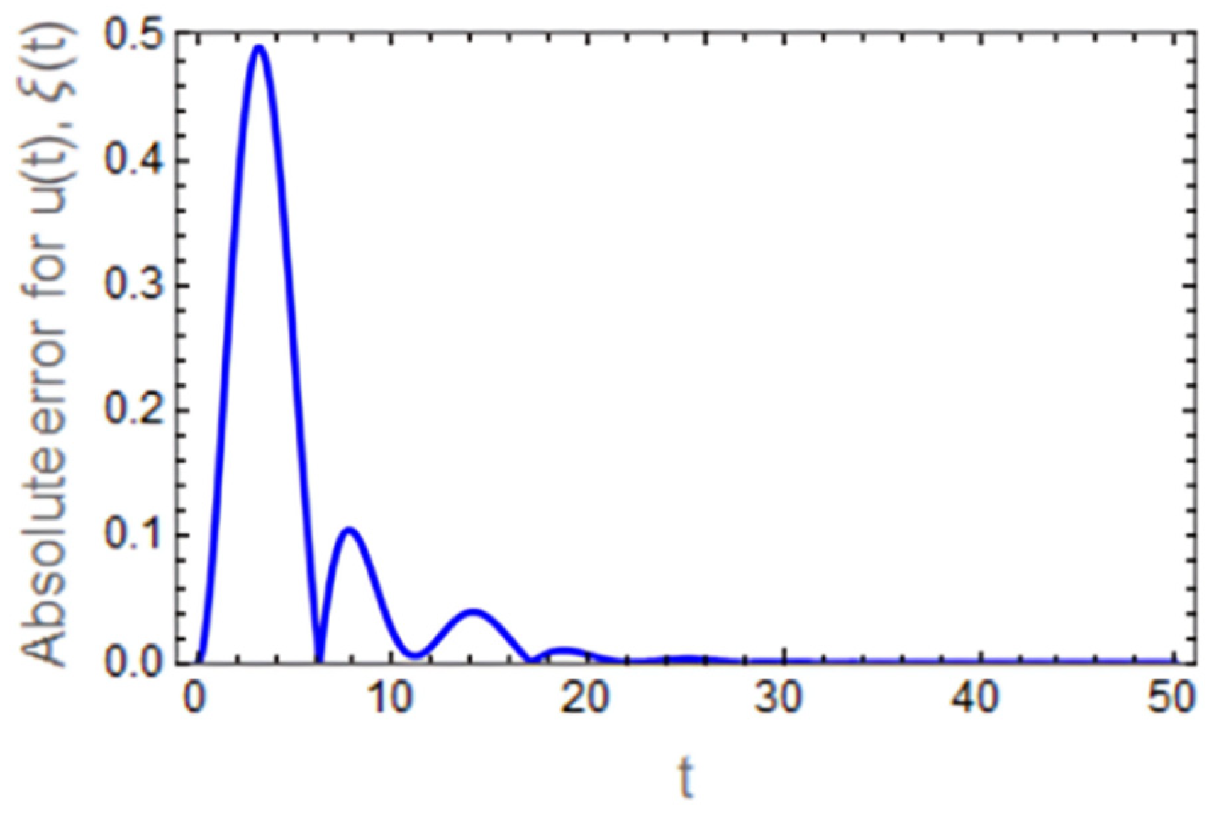
Regrettably, there has yet to be a mathematical derivation pertaining to the NPA. Consequently, the justification for this linearization method, as displayed in Equation (50), arises merely from the remarkable concordance between the nonlinear and linear ODEs. Furthermore, the absolute error curve illustrates the disparity between these two ODEs across the complete domain. Conversely, three primary constraints regarding the NPA can be encapsulated as follows:

i.

The NPA pertains solely to weakly nonlinear oscillators.

ii.

Their ICs remain unaltered.

iii.

To achieve improved accuracy, the initial amplitude of the trial solution should be less than one.

In order to evaluate the natural frequency ω₀ and damping ratio μ₀ of the system, the following assumed solution to Equation (50) is adopted:

$${\eta }_0(t)=A\cos {\Omega }_{0}t.$$

(51)

The natural frequency and damping coefficient are evaluated to construct the linearized model [42,43]:

$${\mu }_0={\displaystyle {\displaystyle \underset{0}{\overset{2\pi /\Omega }{\int }}}{\dot{\eta }}_0^2 D(\eta )dt}/{\displaystyle {\displaystyle \underset{0}{\overset{2\pi /\Omega }{\int }}}{\dot{\eta }}_0^2 dt}=r_1\cos {\theta }_1+{\displaystyle \frac{A^2}{8}}\left(r_3\cos {\theta }_3+2r_5\cos {\theta }_5\right),$$

(52)

$${\omega }_0^2={\displaystyle {\displaystyle \underset{0}{\overset{2\pi /\Omega }{\int }}}{\eta }_0^2 N({\eta }_0)dt}/{\displaystyle {\displaystyle \underset{0}{\overset{2\pi /\Omega }{\int }}}{\eta }_0^2 dt}=r_2\cos {\theta }_2+{\displaystyle \frac{1}{3}}{r}_4\cos {\theta }_4 + {\displaystyle \frac{1}{8}}\left((8h_1+8h_2+6h_3)E^2-3A^2{\Omega }_0^2(c_1+2c_2)+6r_6\cos {\theta }_6\right).$$

(53)

Using the standard normal form, Equation (50) is reduced to a corresponding linearized ODE. The assumed form of the solution is taken as

$$u(t)=u_0(t)Exp(-{\mu }_0 t/2).$$

(54)

and substituting this expression into Equation (50) yields

$$\ddot{u}(t)+{\Omega }_0^{2}u(t)=0,$$

(55)

where ${\Omega }_0^2={\omega }_0^2-{\mu }_0^2/4$, analyzed using MS tools.

Here, ${\mu }_0$ is the effective non-dimensional damping coefficient at $\sigma =0$, while ${\omega }_0$ accounts for the viscous, porous, and viscoelastic dissipation effects.

Within the framework of the equivalent reduced oscillator, the interface remains in a stable oscillatory regime provided that

$${\Omega }_0^2>0, \mathrm{and} {\mu }_0>0.$$

(56)

It should be emphasized that these conditions characterize the behavior of the equivalent reduced oscillator. They distinguish the oscillatory regime from the non-oscillatory regime and should not be interpreted as a complete criterion for the asymptotic stability of the original time-periodic system. Attention is next focused on the functional relationship described by Equations (52) and (53). This relationship is examined by plotting the logarithm of the EF strength as $Log E_0^2$ against the surface wavenumber $k$. 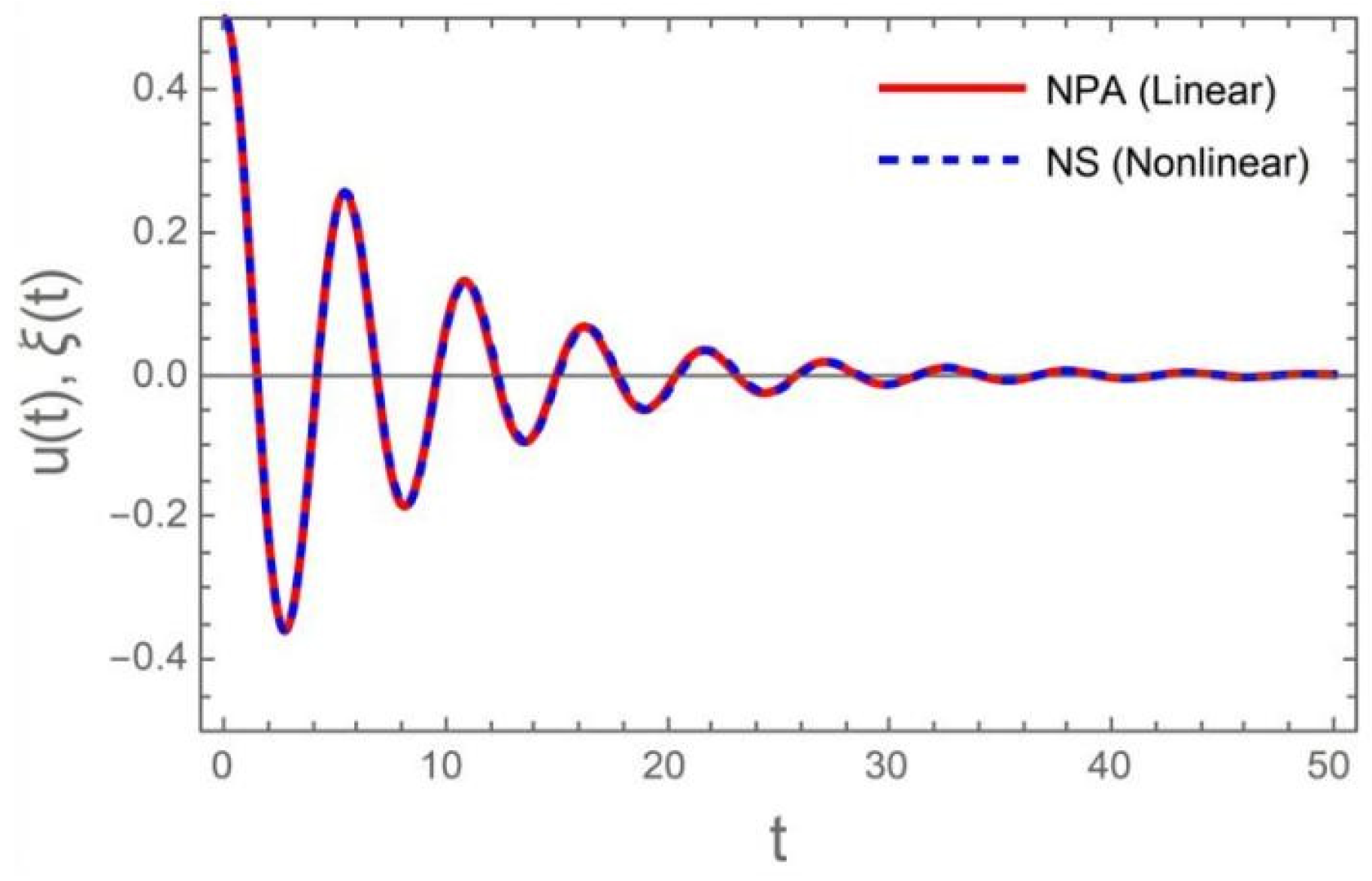The NSs are obtained using the NDSolve routine; meanwhile, analytical approximations are derived from the equivalent linear ODE, as shown in Equation (50). The solution to the original nonlinear Equation (46) is displayed in Figure 2 together with its linear one. Excellent agreement is observed between the numerical and analytical solutions, confirming the accuracy of the adopted approximation and the reliability of the proposed methodology [2,49]. A representative set of parameters used in the computations is listed below:

$$A=\rho =U=\epsilon =0.5, Z=5.0,B_n=\mu =k=D_a=0.2, \nu = We= W_B=\sigma =2.0 \mathrm{and} E^2=5.0.$$

The absolute error curve is provided below for clarity.

Figure 3 presents the variation in the absolute error related to the solution $u(t)$ as a function of time. It is observed that the absolute error initially exhibits relatively high oscillatory values, which can be attributed to the transient behavior of the system and the sensitivity of the solution during the ICs. However, as time progresses, the error rapidly decreases and approaches zero, indicating a strong convergence between the approximate solution and the original nonlinear one. This decay in the absolute error confirms the reliability and accuracy of the adopted linearized model in capturing the system dynamics over time. The results demonstrate that the linear approximation provides an excellent representation of the nonlinear response. In particular, the excellent agreement between the original nonlinear equation and its corresponding reduced model, together with the small absolute errors shown in Figure 2 and Figure 3, provides numerical support for the applicability of the proposed NPA. Furthermore, the extensive parametric investigations presented in Figure 4, Figure 5, Figure 6 and Figure 7 demonstrate the consistency and robustness of the reduced formulation over a broad range of governing parameters.

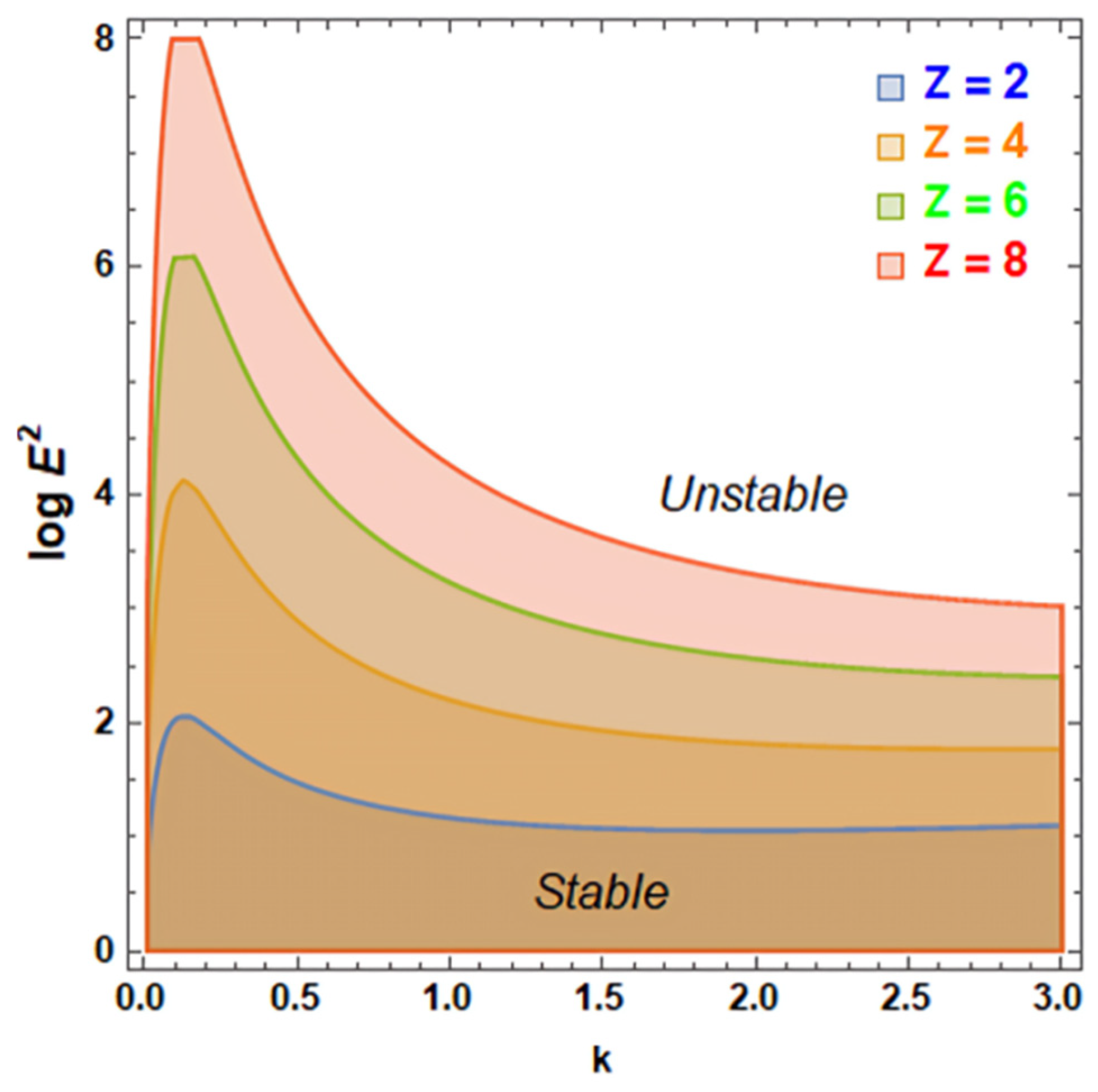
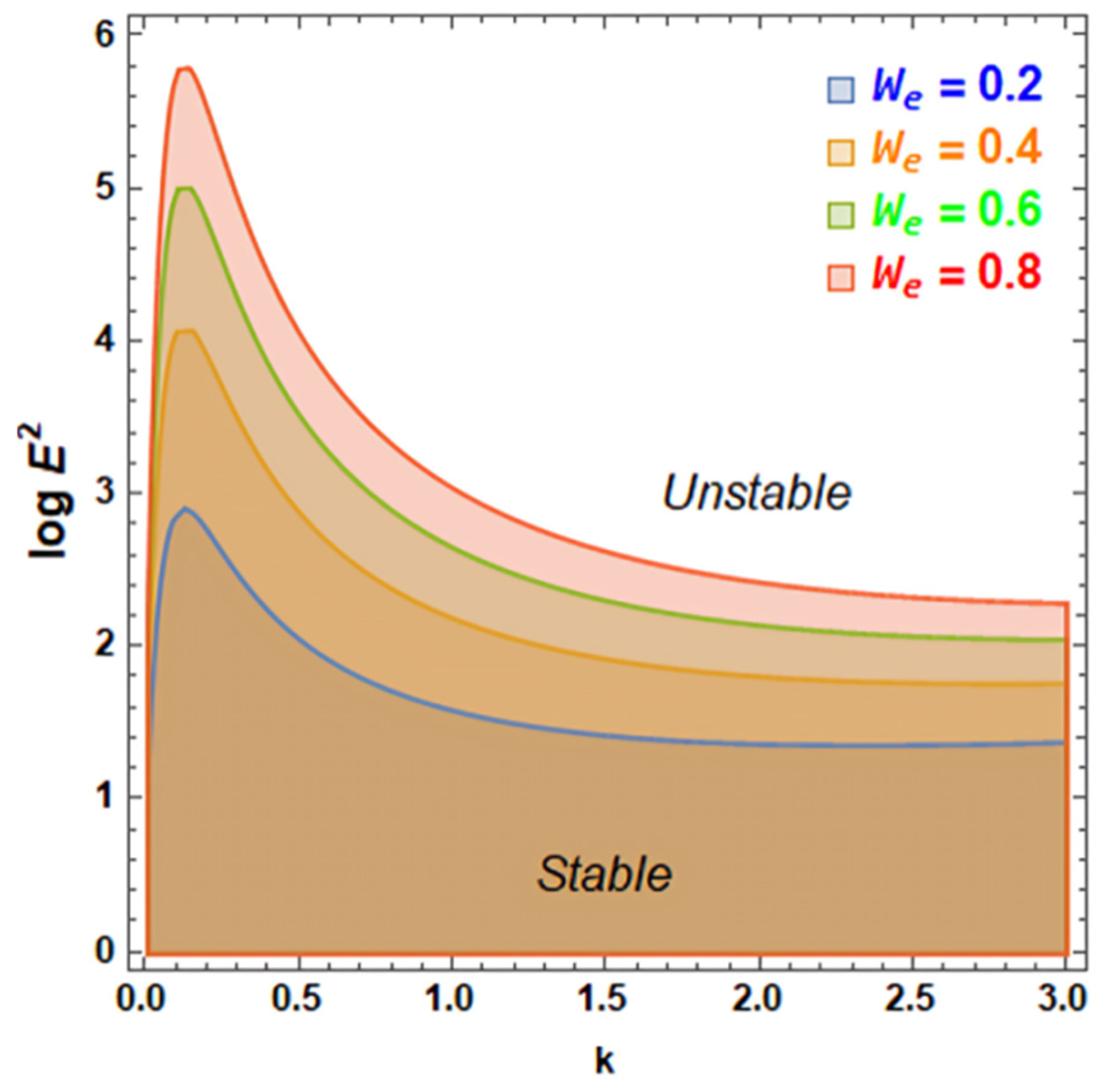
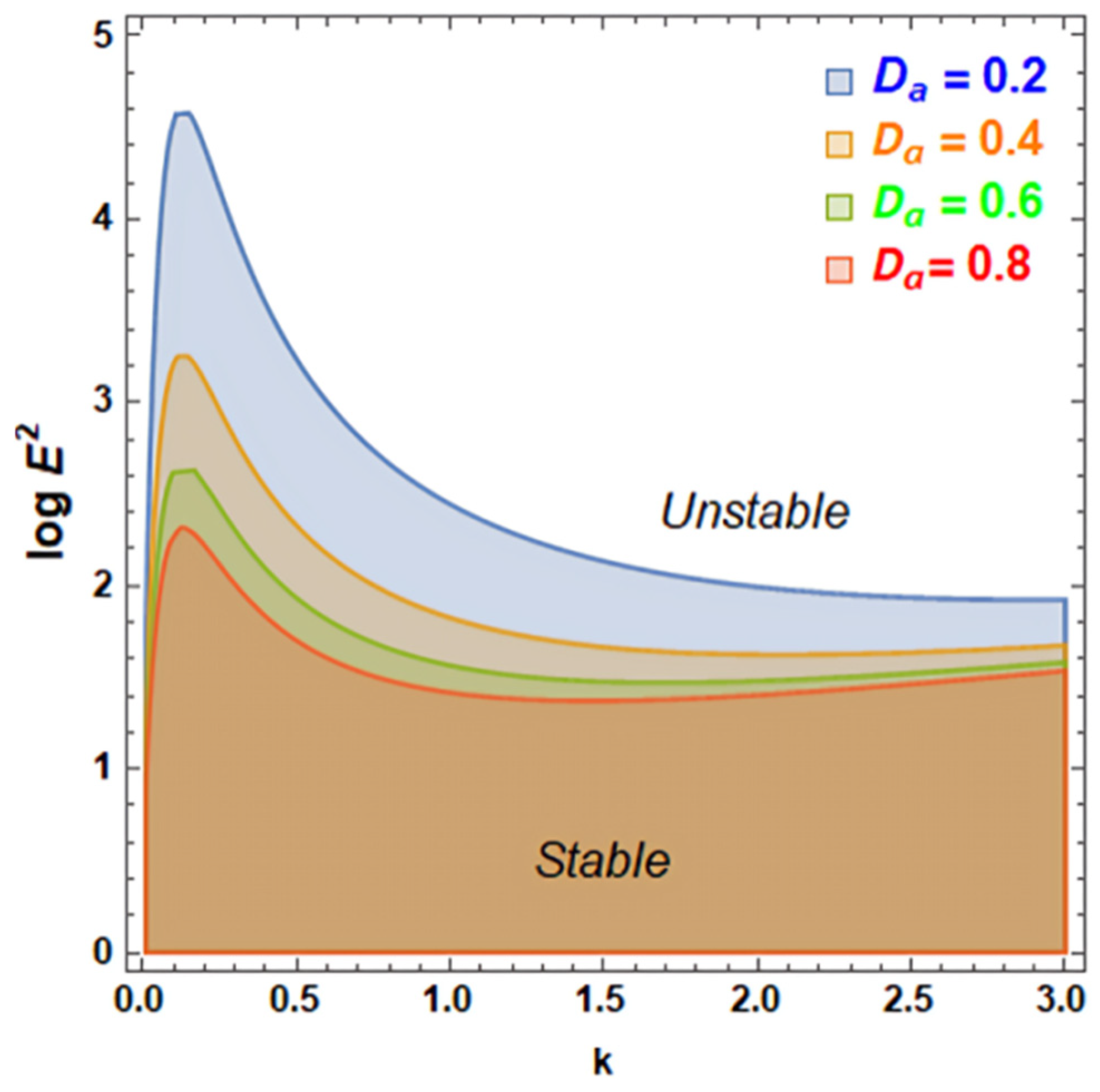
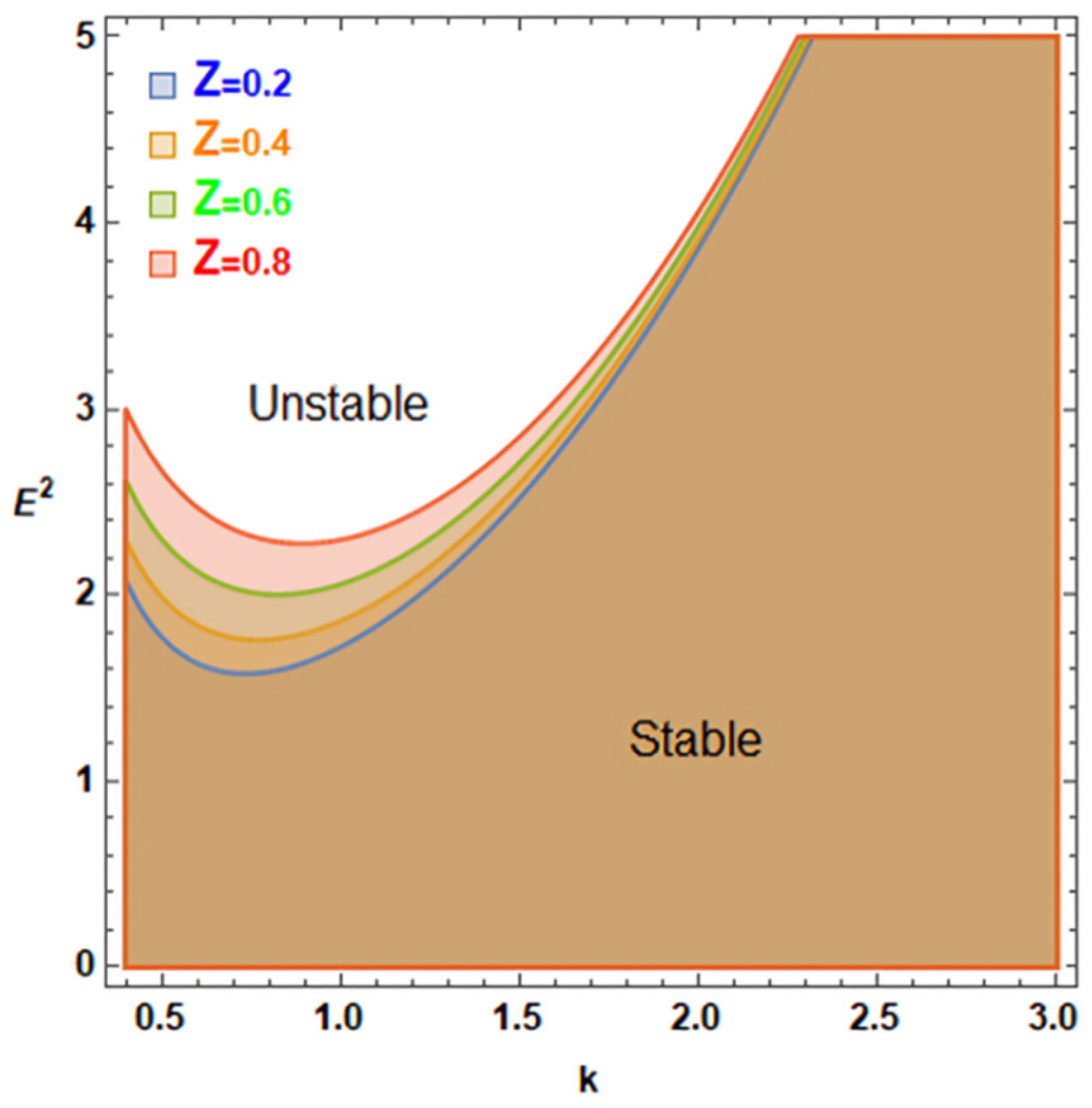
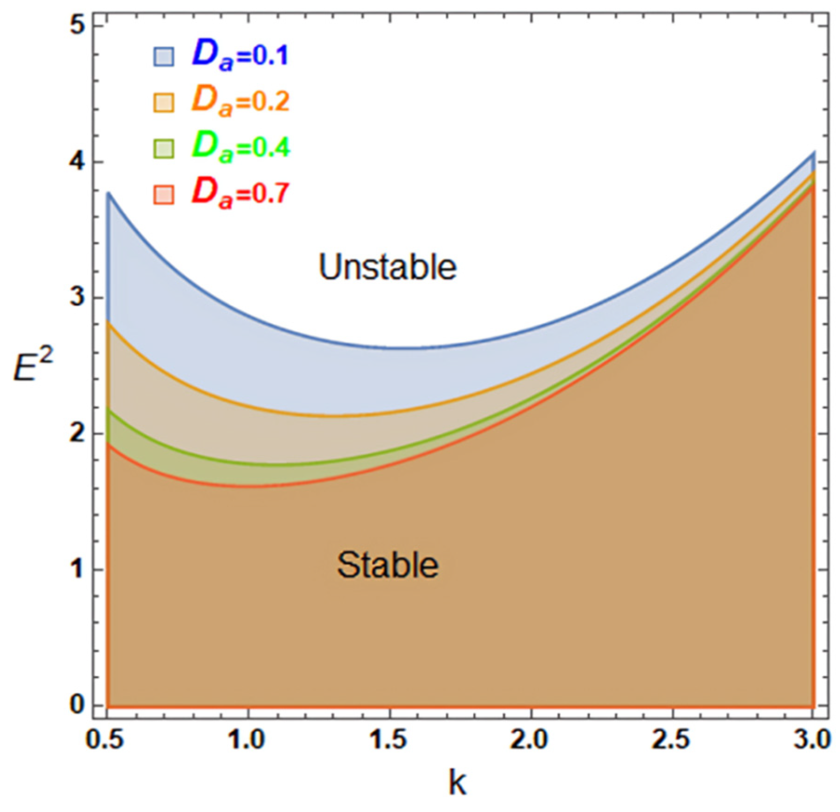
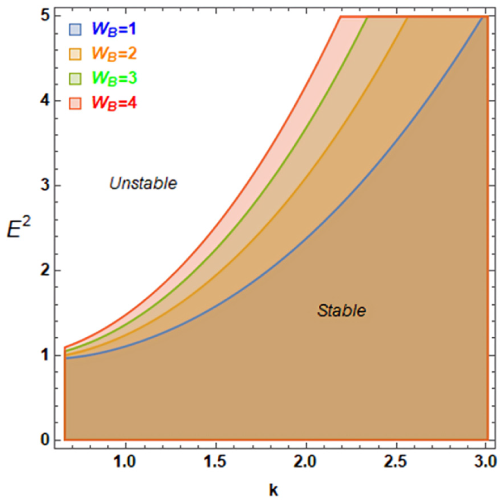
The stability curves for $E^2$ vs. $k$ are presented in Figure 4, Figure 5, Figure 6 and Figure 7. These curves are plotted for selected typical values of the key controlling parameters, where each parameter is varied according to the specific physical effect under consideration in the corresponding figure in order to enhance clarity and efficiency. Based on the stability requirement ${\Omega }_0^2>0,$ the expression of the natural frequency given by Equation (53) serves as a governing factor in shaping the stability boundaries. In particular, the explicit dependence of ${\Omega }_0^2,$ on the EF strength $E_0^2$ and wavenumber k, allows the destabilizing role of the imposed uniform EF to be clearly identified [34].

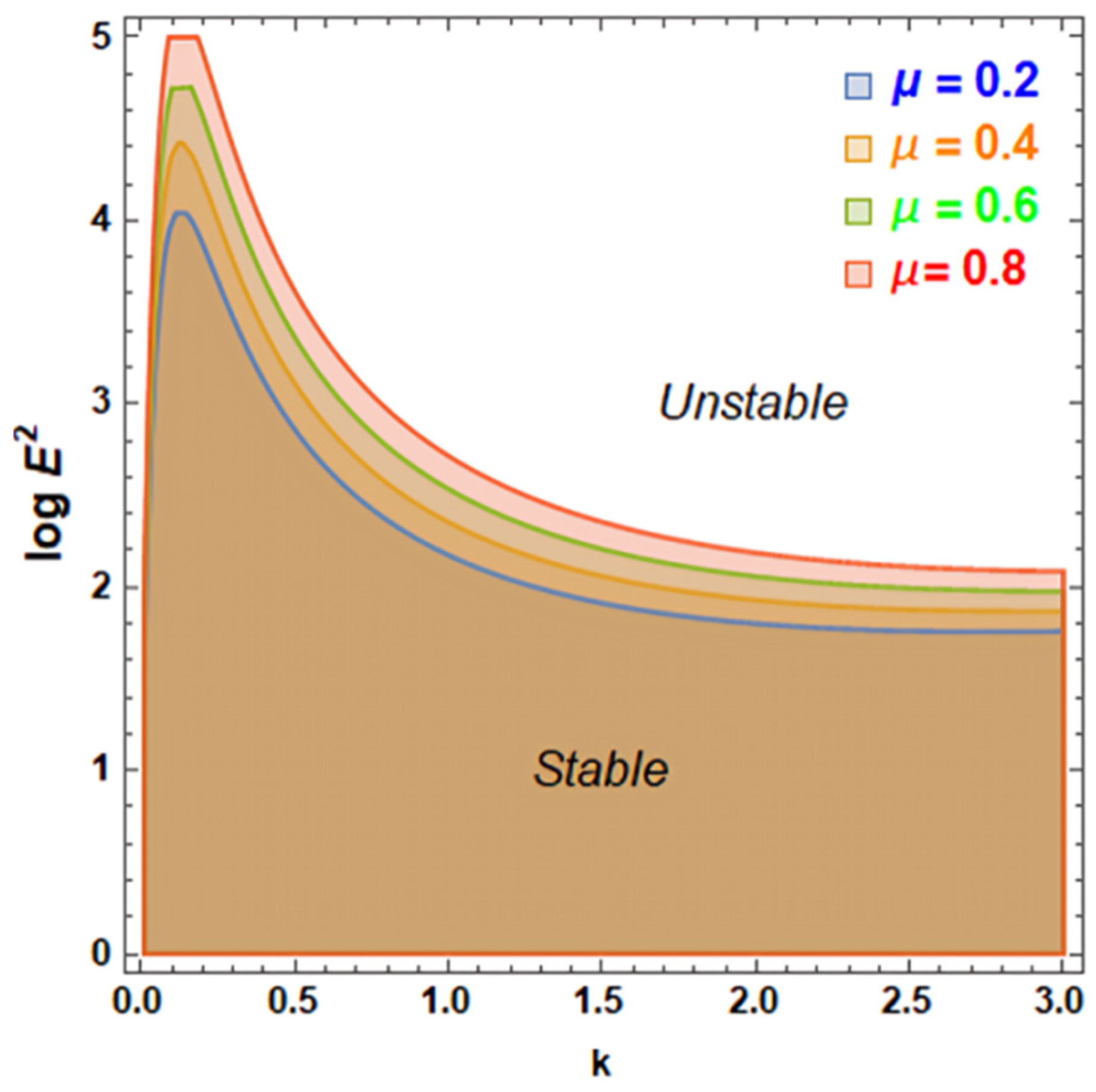
Figure 4 shows the variation induced by the Ohnesorge number Z on the stability characteristics of the system through plots of LogE² versus the wavenumber k. It is observed that increasing Z shifts the stability curves upward, leading to an expansion of the stable region. This stabilizing behavior is attributed to enhanced viscous dissipation, which suppresses the growth in interfacial disturbances. Such an effect by viscous forces on stability is consistent with classical hydrodynamic stability theory [5].

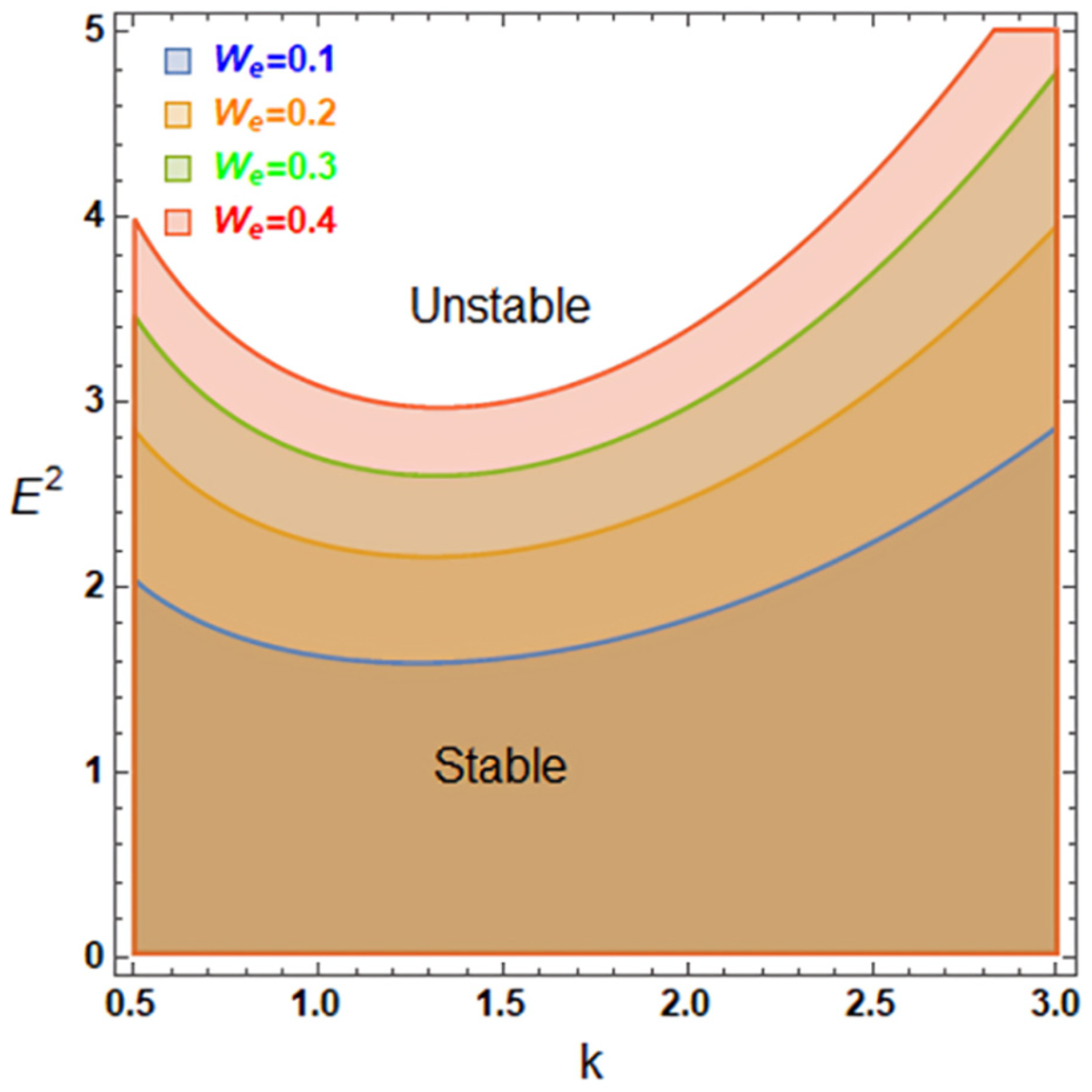
Figure 5 shows the influence of the Weber number W_e on the stability domain. As W_e increases, the stability boundaries move upward, indicating a higher critical EF required for destabilization. Since W_e represents ratio of inertial to ST force effects, larger values imply that ST provides stronger resistance against interface deformation. This stabilizing role of ST was widely reported in stability analyses of interfacial flows [48].

The impact of Darcy number D_a on system stability is depicted in Figure 6. Unlike the previous parameters, the increasing D_a causes a downward shift in the stability curves and a reduction in the stable region. Physically, higher D_a corresponds to increased permeability of the porous medium, which reduces flow resistance and facilitates disturbance propagation. This destabilizing influence of porous medium permeability was well documented in studies of stability in porous systems [50].

Figure 7 presents the effect of the kinematic viscosity μ on the stability behavior of the system. The increasing μ results in an upward shift in the stability curves, indicating enhanced system stability. Higher viscosity increases energy dissipation and attenuates velocity fluctuations associated with perturbations, thereby delaying the onset of instability. This stabilizing influence of viscous effects is in agreement with classical fluid dynamics analyses [50].

Generally, the stability behavior of the system results from a competition among destabilizing effects associated with the porous medium permeability, represented by the Darcy number D_a, and stabilizing mechanisms arising from viscous dissipation and ST effects, represented by Z, W_e, and μ.

5.1. General Case of Periodic EF as $\sigma \ne 0$

The nonlinear Mathieu oscillator, as shown in Equation (42), contains both quadratic and cubic functions. The system becomes non-autonomous as a result of excitation frequency disturbances, caused by parametric excitation. Nevertheless, by replacing the modified natural frequencies with an effective constant frequency, the system can evolve into an autonomous regime. This approach was previously reported [51,52,53]. Consequently, Equation (42) can be rewritten as an autonomous structure:

$$\ddot{\eta }+r_1\cos {\theta }_1\dot{\eta }+Q_1^2(\sigma )\eta +c_1\eta \ddot{\eta }+r_3\cos {\theta }_3\eta \dot{\eta }+Q_2^2(\sigma ){\eta }^2+c_2{\eta }^2\ddot{\eta }+r_5\cos {\theta }_5{\eta }^2\dot{\eta }+Q_3^2(\sigma ){\eta }^3=0 .$$

(57)

The transformation to an autonomous equation, free from variable coefficients, allows for a more straightforward examination of the system’s dynamic behavior. This reformulation greatly eases the analysis of both the stability and resonance phenomena. It should be noted that the transformation of the time-periodic system into an autonomous form represents an approximate averaging procedure. Consequently, the obtained stability conditions describe the behavior of the reduced system and do not capture the full parametric resonance structure that would arise from a complete Floquet analysis. The corresponding constant-coefficient formulas for $\eta ,\dot{\eta } \mathrm{and} \ddot{\eta }$ are given below [54]:

$$Q_1^2(\sigma )={\displaystyle {\displaystyle \underset{0}{\overset{2\pi }{\int }}}({\cos }^{2}t)(r_2\cos {\theta }_2-d_1{\cos }^2\sigma t)dt}/{\displaystyle {\displaystyle \underset{0}{\overset{2\pi }{\int }}}({\cos }^{2}t)dt}=r_2\cos {\theta }_2+{\displaystyle \frac{1}{2}}{d}_1\left(1+{\displaystyle \frac{(2{\sigma }^2-1)\sin (4\pi \sigma )}{4\pi \sigma ({\sigma }^2-1)}}\right),$$

(58)

$$Q_2^2(\sigma )={\displaystyle {\displaystyle \underset{0}{\overset{2\pi }{\int }}}({\cos }^{2}t)(r_4\cos {\theta }_4-d_2{\cos }^2\sigma t)dt}/{\displaystyle {\displaystyle \underset{0}{\overset{2\pi }{\int }}}({\cos }^{2}t)dt}=r_4\cos {\theta }_4-{\displaystyle \frac{1}{2}}{d}_2\left(1+{\displaystyle \frac{(2{\sigma }^2-1)\sin (4\pi \sigma )}{4\pi \sigma ({\sigma }^2-1)}}\right),$$

(59)

and

$$Q_3^2(\sigma )={\displaystyle {\displaystyle \underset{0}{\overset{2\pi }{\int }}}({\cos }^{2}t)(r_6\cos {\theta }_6-d_3{\cos }^2\sigma t)dt}/{\displaystyle {\displaystyle \underset{0}{\overset{2\pi }{\int }}}({\cos }^{2}t)dt}=r_6\cos {\theta }_6+{\displaystyle \frac{1}{2}}{d}_3\left(1+{\displaystyle \frac{(2{\sigma }^2-1)\sin (4\pi \sigma )}{4\pi \sigma ({\sigma }^2-1)}}\right).$$

(60)

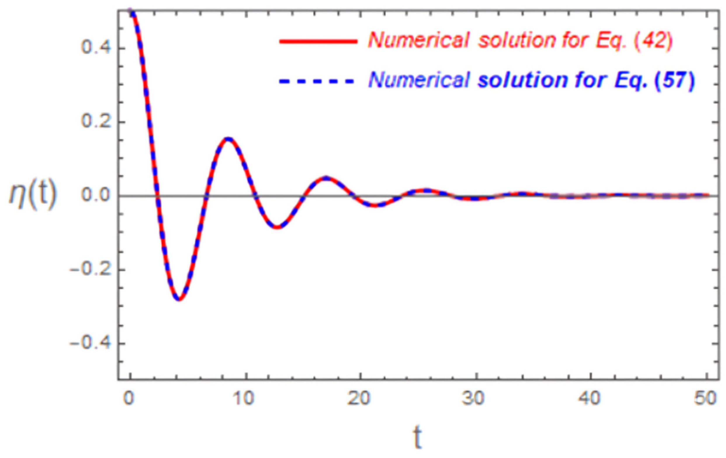
The NS is provided for the comparison between Equations (42) and (57). The following data sample is used in conjunction with the computation:

$$A=\epsilon =0.5, Z=5,\rho =B_n=\mu =k=0.2, D_a=0.6, U=0.5,\nu = We= W_B=\sigma =2 \mathrm{and} E^2=10.$$

The Figure 8 shows that the solutions agree well, with an estimated relative error of 0.000486527.

To preserve the core dynamical behavior of the original nonlinear system, a revised formulation is introduced that explicitly accounts for the quadratic nonlinearity. This approach provides a clearer and more insightful framework for understanding the system response. El-Dib [46] was the first to incorporate a quadratic stiffness contribution into the constitutive relationship, enabling evaluation of the system frequency and the construction of the associated solution while explicitly considering the effects of quadratic nonlinearity. This was achieved through the inclusion of a cubic term rather than a quadratic one while completing the integration with regard to the variable $\eta$. Consequently, Equation (57) can be rewritten to indicate that the restoring force embodies the effects of the quadratic nonlinearity influence, as follows:

$$\ddot{\eta }+G_0(\eta )\dot{\eta }+G_1(\eta )\eta =0 ,$$

(61)

where

$$G_0(\eta )=r_1\cos {\theta }_1+\left({\displaystyle \frac{1}{2}}{r}_3\cos {\theta }_3+r_5\cos {\theta }_5\right){\eta }^2 ,$$

(62)

and

$$G_1(\eta )=Q_1^2(\sigma )+\left({\displaystyle \frac{1}{2}}{c}_1+c_2\right)\eta \ddot{\eta }+\left({\displaystyle \frac{1}{3}}{Q}_2^2(\sigma )+Q_3^2(\sigma )\right){\eta }^2 .$$

(63)

The temporal evolution of interfacial disturbance is governed by the nonlinear ODE given in Equation (61), which summarizes several important dynamical features of the system. The combined effects of porous resistance and viscoelasticity are incorporated through the function $G_0(\eta )\dot{\eta }$, which functions as an effective damping mechanism with a strength that varies according to the instantaneous displacement. Meanwhile, the restoring force represented by $G_1(\eta )\eta$ combines EHD and elastic contributions, leading to a stiffness mechanism whose dependence on displacement modifies the system’s inherent dynamic oscillations. The periodic modulation introduced by the time-dependent EF further enriches the system dynamics, giving rise to the system response, which may range from purely oscillatory to weakly damped motions depending on the chosen parameter values. Consequently, the interface behaves as a damped, periodically driven nonlinear oscillator, with its stability, amplitude, and dominant frequency determined by the interplay between EF forcing, porous medium resistance, viscoelastic effects, and inertia.

To facilitate analytical treatment and establish a direct connection with the stability analysis, the nonlinear Equation (61) is reformulated by consistently reorganizing the quadratic nonlinearities so that they primarily affect the restoring force. This reformulation preserves the essential nonlinear dynamics while improving tractability. Consequently, Equation (61) admits an equivalent linear framework that retains the dominant oscillatory characteristics of the system. In the general case of a periodic EF, this linearized governing ODE differs from the uniform EF case only due to the explicit time dependence of the electric excitation; meanwhile, the damping mechanism remains physically identical. Accordingly, the governing linear ODE can be written as

$$\ddot{u}+{\mu }_{eq}\dot{u}+{\omega }_{eq}^{2}u=0 .$$

(64)

To determine the equivalent natural frequency ${\omega }_{eq}$ and damping coefficient ${\mu }_{eq}$, a trial solution satisfying the same admissibility ICs as previously stated is assumed in the following form:

$${\eta }_0(t)=A\cos \Omega t .$$

(65)

The total frequency Ω will be specified later.

Following the same averaging procedure adopted in the uniform EF case, the equivalent damping coefficient is evaluated as

$${\mu }_{eq}={\displaystyle {\displaystyle \underset{0}{\overset{2\pi /\Omega }{\int }}}{\dot{\eta }}_0^2 G_0({\eta }_0)dt}/{\displaystyle {\displaystyle \underset{0}{\overset{2\pi /\Omega }{\int }}}{\dot{\eta }}_0^2 dt}=r_1\cos {\theta }_1+{\displaystyle \frac{A^2}{8}}\left(r_3\cos {\theta }_3+2r_5\cos {\theta }_5\right),$$

(66)

It is worth noting that the damping coefficient retains the same structure as in the uniform EF case, reinforcing the consistency of the formulation. The equivalent natural frequency corresponding to the periodic EF is determined as

$${\omega }_{eq}^2={\displaystyle {\displaystyle \underset{0}{\overset{2\pi /\Omega }{\int }}}{\eta }_0^2 G_1({\eta }_0)dt}/{\displaystyle {\displaystyle \underset{0}{\overset{2\pi /\Omega }{\int }}}{\eta }_0^2 dt}={\displaystyle \frac{1}{8}}\left(3A^2{\Omega }^2(c_1+2c_2)-2(4Q_1^2(\sigma )+Q_2^2(\sigma )+3Q_3^2(\sigma ))\right).$$

(67)

In order to eliminate the first-order time derivative term in Equation (64), the standard normal form transformation is applied. This transformation removes the damping term from the equation for $u(t)$ and converts the governing ODE into an undamped second ODE with modified frequency.

The solution is therefore assumed as

$$u(t)=A{e}^{-{\mu }_{eq}t/2}\left(\cos \Omega t+{\displaystyle \frac{{\mu }_{eq}}{2\Omega }}\sin \Omega t\right).$$

(68)

The total frequency associated with the transformed system is then given by

$${\Omega }^2={\omega }_{eq}^2-{\mu }_{eq}^2/4.$$

(69)

Substituting Equations (66) and (67) into Equation (69) yields the following quadratic frequency equation:

$${\Omega }^2\left(8-3A^2(c_1+2c_2)\right)+2\left((r_1\cos {\theta }_1\right.+{\displaystyle \frac{1}{8}}{A}^2{r}_3\cos {\theta }_3+2r_5\cos {\theta }_5{)}^2+4Q_1^2(\sigma )+Q_2^2(\sigma )+3Q_3^2(\sigma ))=0.$$

(70)

For the equivalent reduced system to remain in a stable oscillatory regime, the following condition must be satisfied:

$$\left(8-3A^2(c_1+2c_2)\right)\left((r_1\cos {\theta }_1\right.+{\displaystyle \frac{A^2}{8}}{r}_3\cos {\theta }_3+2r_5\cos {\theta }_5{)}^2+4Q_1^2(\sigma )+Q_2^2(\sigma )+3Q_3^2(\sigma ))<0.$$

(71)

The above condition is derived from the reduced autonomous model obtained through the transformation procedure. Therefore, it describes the stability characteristics of the averaged system and does not fully capture the parametric resonance structure that may arise in the original periodically forced system.

5.2. Numerical Discussions

This subsection discusses how the final analytical solution found in Equation (68) is affected by physical elements that guide the mathematical model. Therefore, the numerical evaluation of the solution under the combined influences of the following exemplary system configuration $\sigma , D_a, Z, We, W_B \mathrm{and} \epsilon$:

$$A=\rho =U=\sigma = \mu =0.5, Z=0.8,B_n=\epsilon =W_B=0.2,k=1.5, D_a=6, \nu = 2 ,We=0.1 \mathrm{and} E^2=5.$$

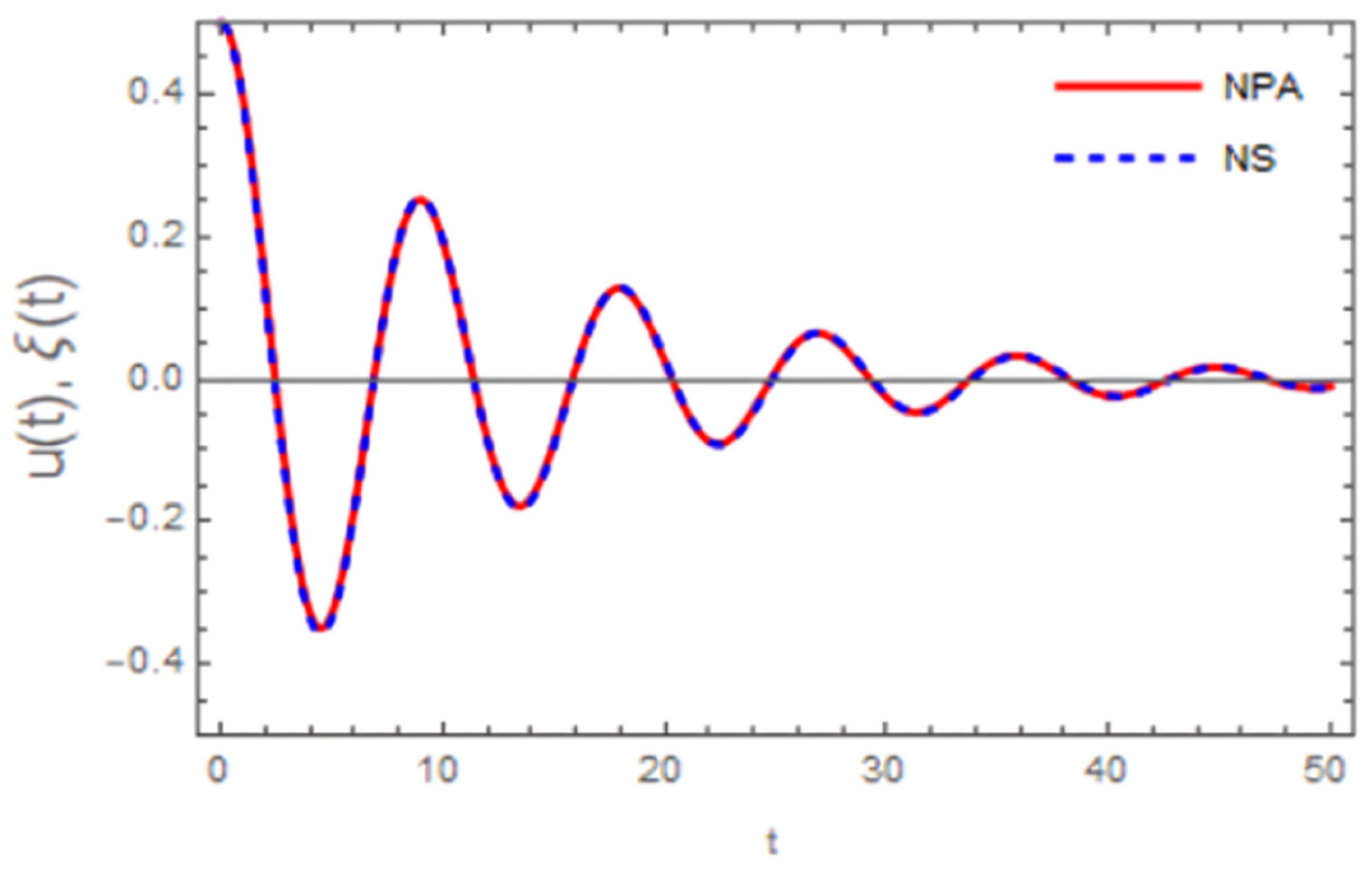
The NS of the nonlinear ODE given by Equation (45), represented by the red curve, and the corresponding linearized solution obtained from Equation (64), represented by the blue curve, are compared in Figure 9. Excellent agreement is observed between the nonlinear and linearized formulations, as evidenced by the close correspondence of the two curves. The small discrepancies observed over the considered time interval confirm the accuracy and reliability of the adopted numerical approach. This agreement indicates that the reduced model successfully captures the essential dynamics of the original nonlinear system and provides an accurate approximation of its behavior.

For a clearer illustration, the related absolute error curve is described below.

The documented absolute error values remain adequately minimal across the full spectrum of the examined parameters, indicating the exceptional precision and dependability of the suggested analytical solution. The most significant absolute error recorded is merely a few hundredths, while the other errors are many magnitudes smaller, demonstrating remarkable concordance between the analytical forecasts and the relevant reference or NSs. The magnitude of such errors falls well within the standard tolerances typically accepted in engineering and physical modeling and does not affect the qualitative or quantitative patterns of the outcomes. To elucidate this matter, an explanatory note has been incorporated into the updated text highlighting that these minor absolute errors affirm the validity, convergence, and robustness of the suggested formulation over the examined parameter ranges. 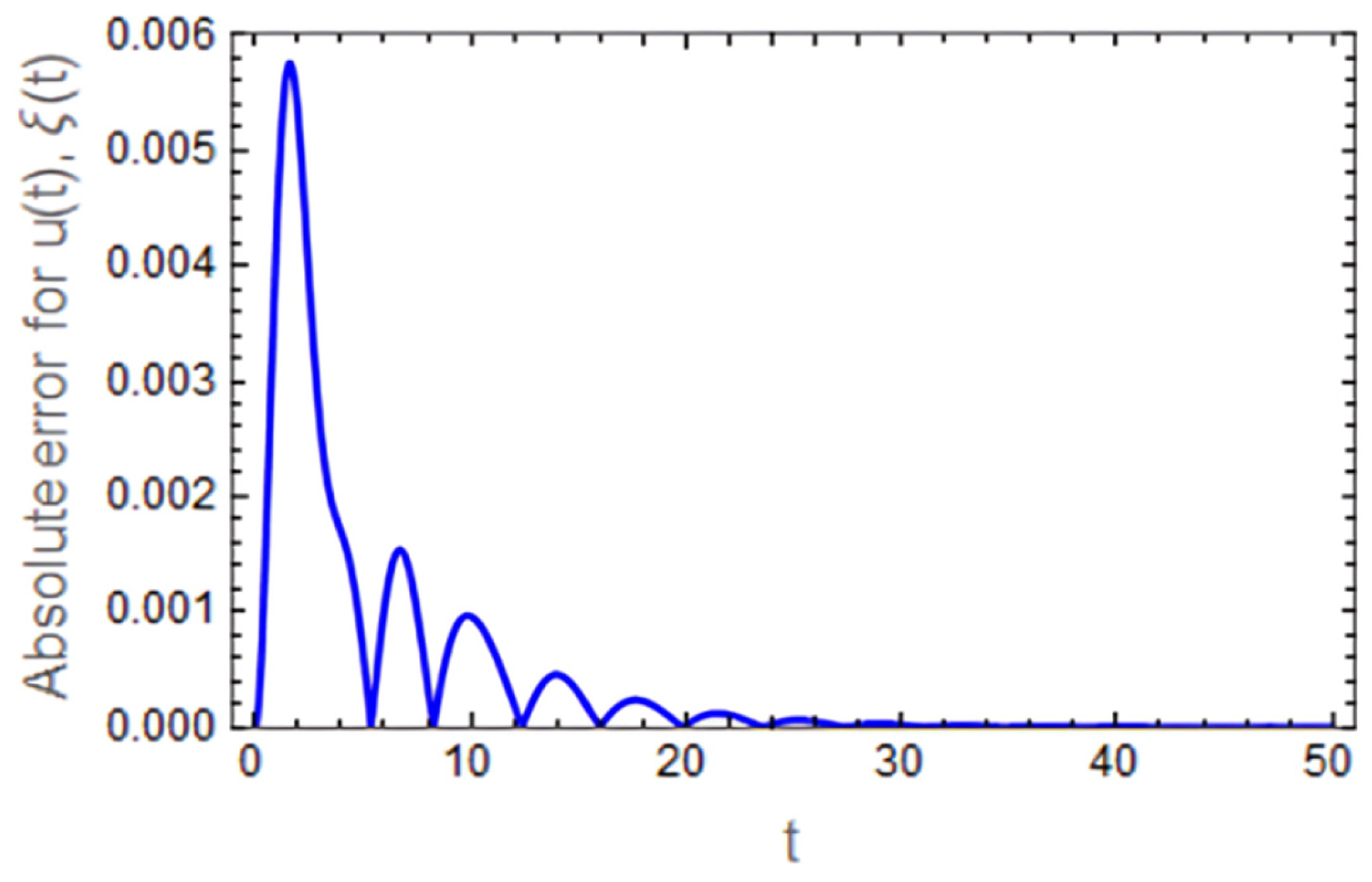Figure 10 illustrates the time history of the absolute error associated with the solution $u(t)$. It is observed that the absolute error attains relatively higher values at the initial stage due to the transient response of the system and the initial sensitivity of the solution. As time progresses, the absolute error decreases rapidly in an oscillatory manner and eventually approaches zero. This behavior indicates a strong convergence between the approximate (linearized) solution and the original nonlinear solution. The small magnitude of the absolute error over the entire time interval demonstrates the high accuracy of the proposed approximation and confirms its effectiveness in capturing the essential dynamics of the system. The excellent agreement between the NSs of the original nonlinear ODE and the corresponding reduced model, together with the very small absolute errors shown in Figure 8, Figure 9 and Figure 10, provides numerical support for the applicability of the proposed approximation. Moreover, the subsequent parametric investigations and stability diagrams indicate that the reduced model yields physically consistent predictions over a broad range of governing parameters, including E², $D_a$, Z, $We$, $W_B$, and σ.

.

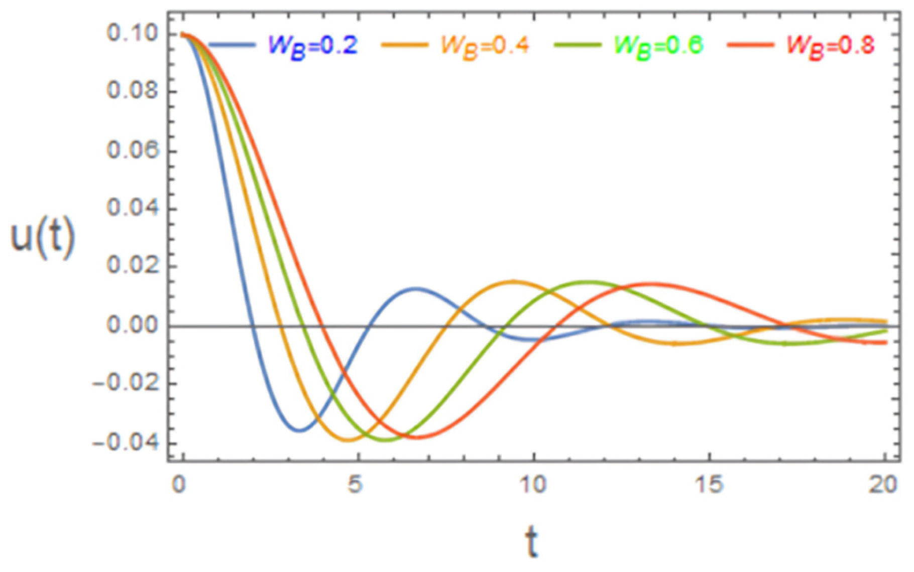
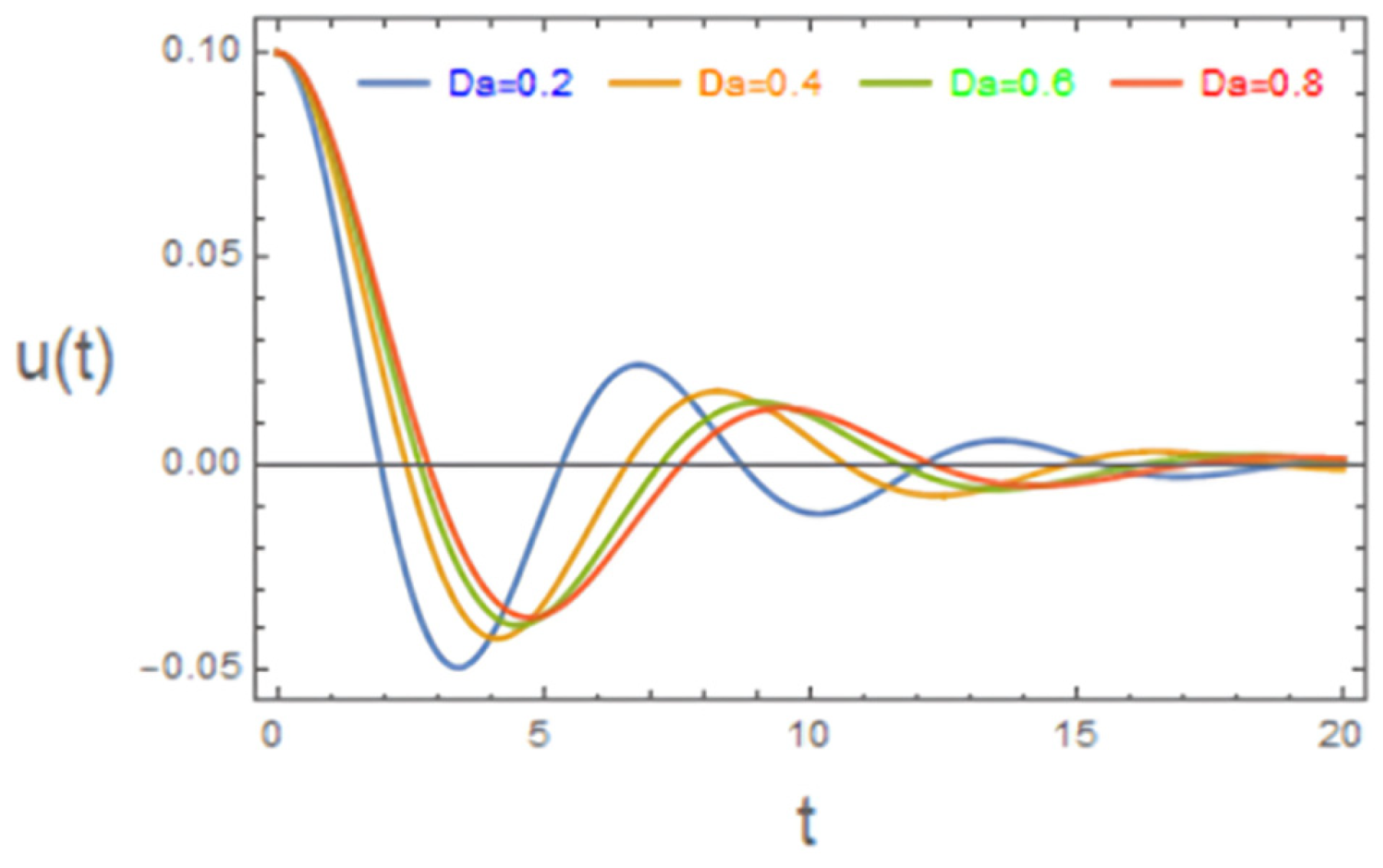
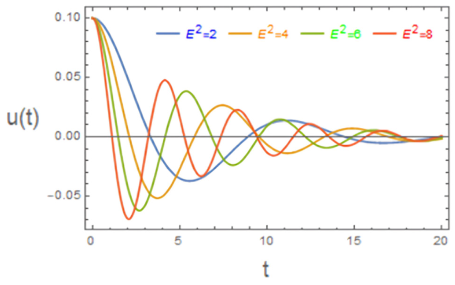
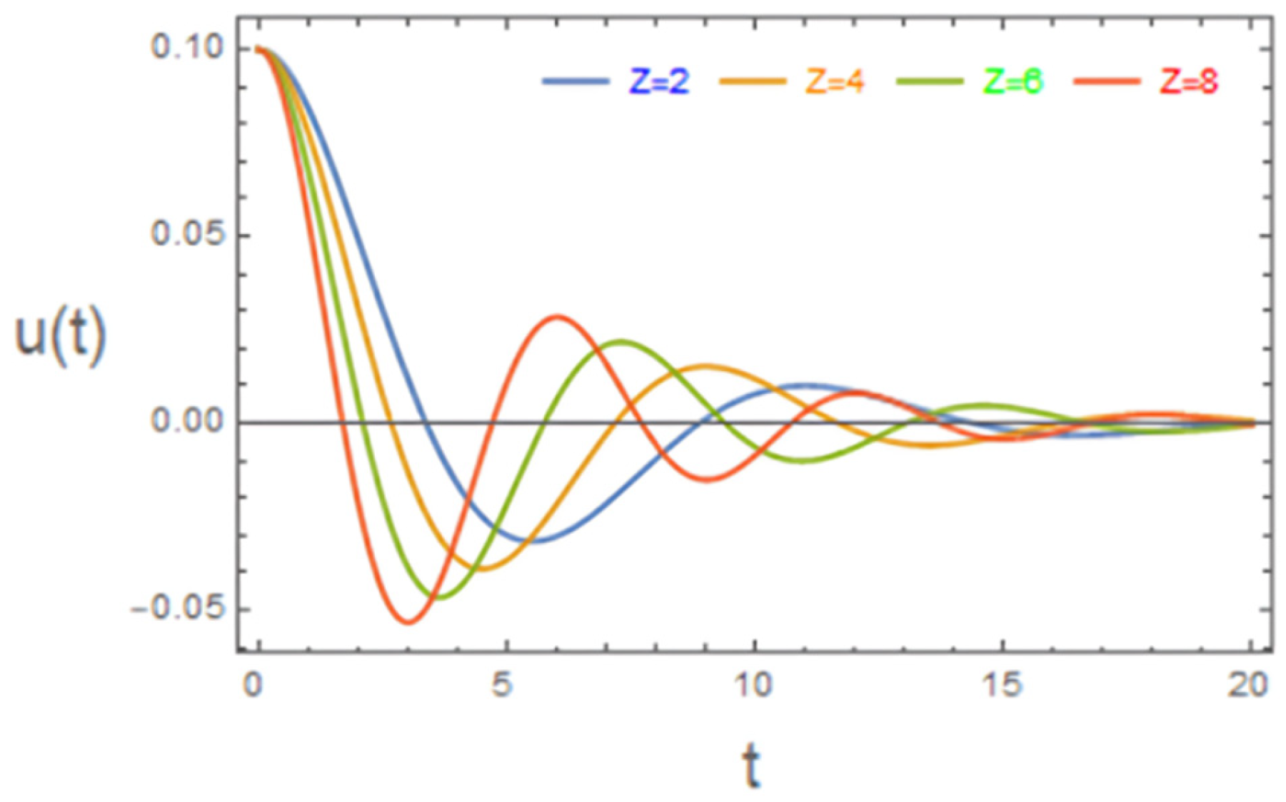
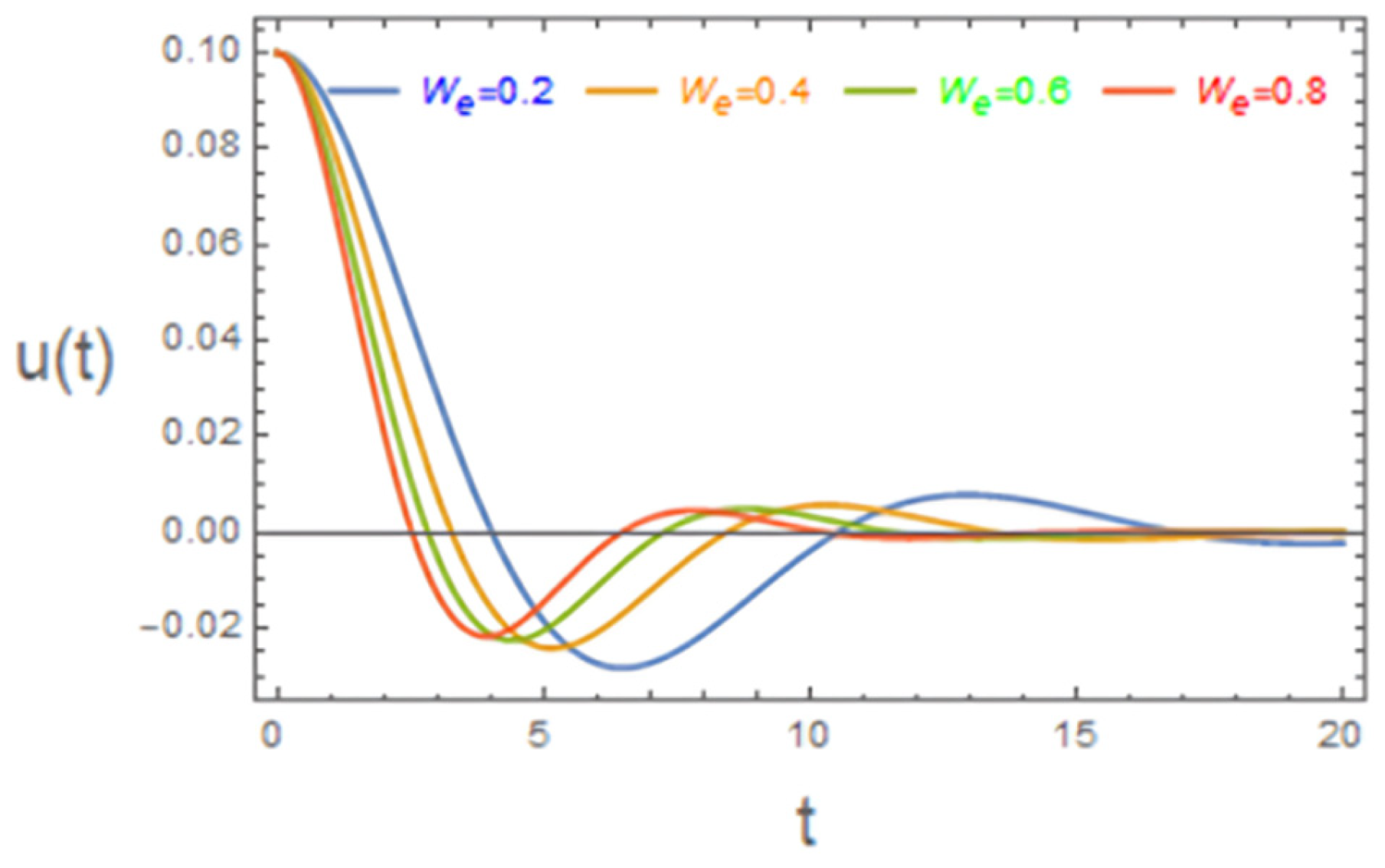
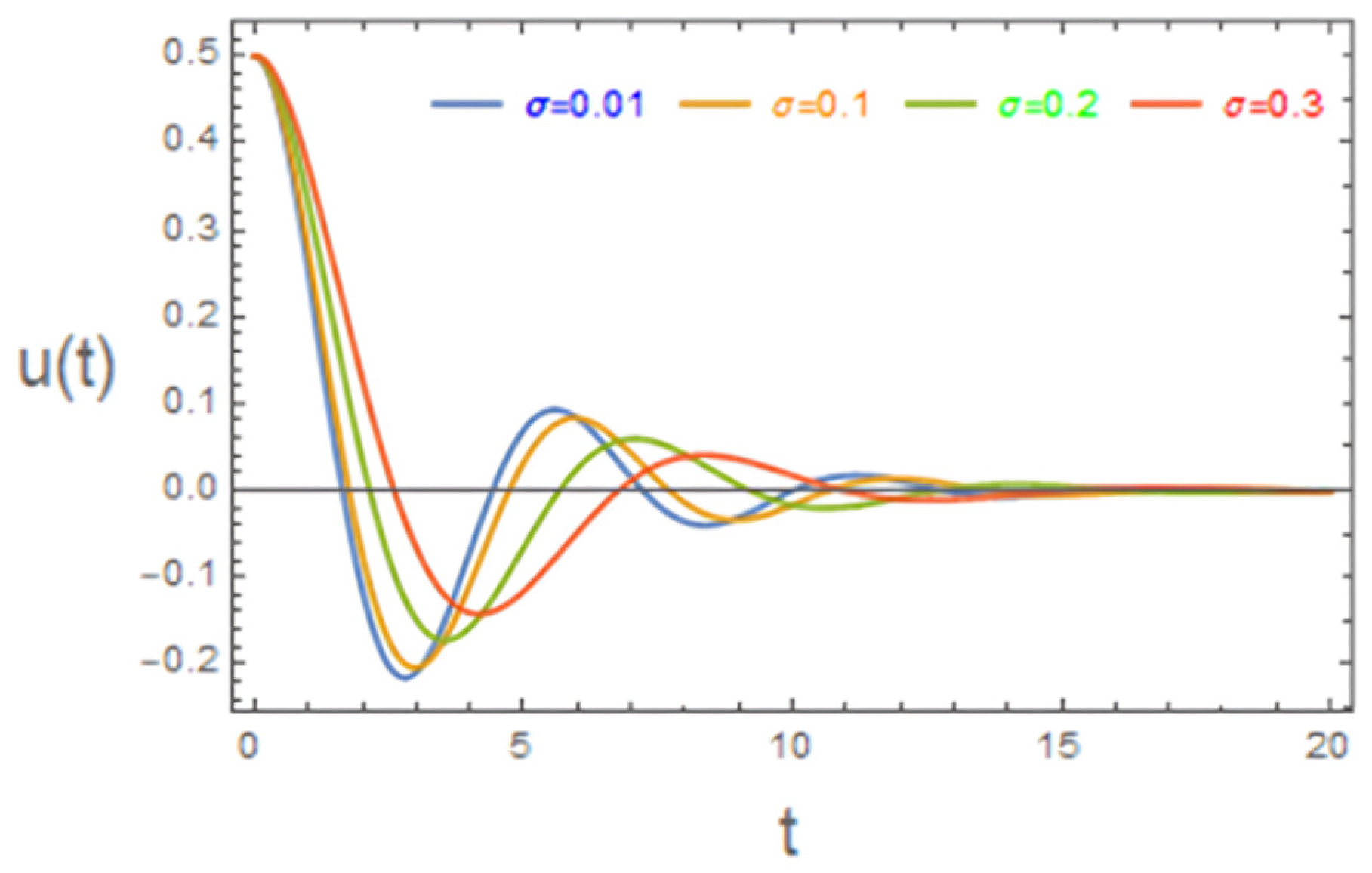
Figure 11, Figure 12, Figure 13, Figure 14, Figure 15 and Figure 16 collectively demonstrate that the temporal evolution of the electrified interface is governed by the competition between energy injection mechanisms and dissipative/restoring effects. The EF parameters, represented by the forcing-frequency parameter σ and the EF intensity E², primarily control the amount and manner of energy transferred to the interface. Increasing E² produces the strongest amplification of the oscillatory response, resulting in larger amplitudes and more persistent oscillations, which reflects the destabilizing action of Maxwell stresses. In contrast, variations in σ mainly modify the oscillation pattern through changes in phase and modulation characteristics, indicating the importance of the frequency matching between the periodic electric forcing and the natural dynamics of the interface.Such behavior is consistent with classical and contemporary studies of EHD instability and periodically forced EF systems [2,3,20].

The influence of the porous medium is represented by the Darcy number D_a. Larger values of D_a, corresponding to higher permeability, reduce the resistance offered by the porous matrix and therefore allow disturbances to propagate more efficiently. As a result, the oscillatory response becomes less damped and persists for longer. This behavior reveals that porous resistance acts as an additional dissipation mechanism capable of suppressing interface motion, in agreement with previous investigations on porous-medium flow stability [8,35,49,50].

Opposing these destabilizing effects are the viscous, elastic, and capillary restoring mechanisms represented by Z, W_B, and We, respectively. An increase in the Ohnesorge number Z enhances viscous dissipation and accelerates the decay of oscillations. Similarly, larger values of W_B introduce stronger elastic restoring stresses that resist interface deformation and reduce oscillation amplitudes. ST effects, characterized by We, also contribute to stabilization by suppressing wave growth and limiting the persistence of interfacial disturbances. These trends are consistent with established theories of viscous, viscoelastic, and capillary stabilization mechanisms [5,6,14,15,39,42].

Overall, the temporal responses reveal that the system behavior is dominated by a balance between EF excitation (E² and σ) and stabilizing mechanisms associated with viscosity Z, elasticity W_B, surface tension We, and porous resistance (low D_a). Among these parameters, E² appears to exert the most direct influence on oscillation amplification, whereas Z, W_B, and We mainly control the damping characteristics of the response. These observations are consistent with established studies of nonlinear EHD interfacial dynamics [11,16,18,20,36].

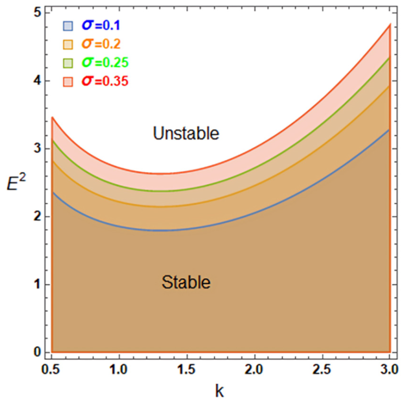
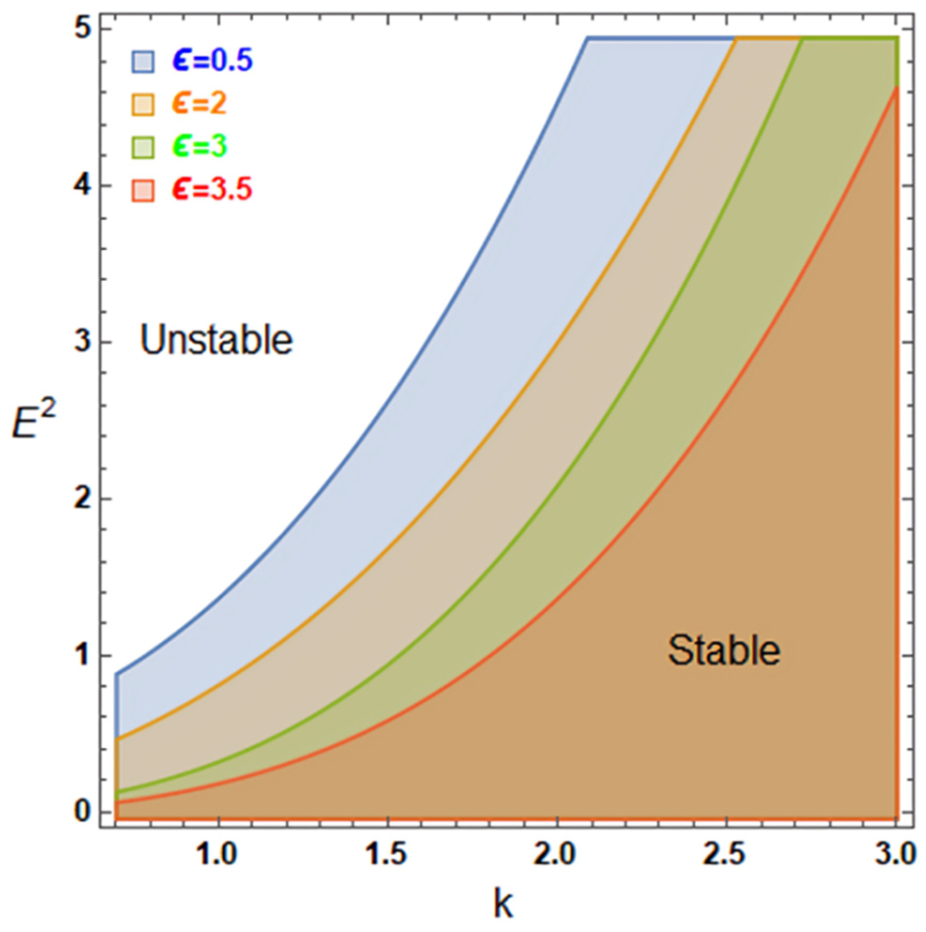
Subsequently, Figure 17, Figure 18, Figure 19, Figure 20, Figure 21 and Figure 22 show the stability layout of the system, stressing the importance of analyzing the stability of the derived solution that defines the vibration pattern. The system in question is evaluated against the stability criterion outlined in Equation (71), and the resultant configuration is presented as follows:

$$A=2,\rho =U= \mu =W_B=\epsilon =0.5, \sigma =0.02, Z=0.8,B_n=5, k=1.2, D_a=0.2, \nu = 2,We=0.1 \mathrm{and} E_0^2=10$$

In these figures, the word “unstable” denotes the unstable region, whereas the shaded portion of the graph with the label “stable” represents the stable region.

The stability diagrams presented in Figure 17, Figure 18, Figure 19, Figure 20, Figure 21 and Figure 22 provide a unified picture of how the governing parameters modify the critical EF intensity required for instability. A common feature in all cases is that the stability boundary reflects the balance between destabilizing electric stresses and the various restoring or dissipative mechanisms acting on the interface, which is a central concept in electrohydrodynamic stability theory [2,3,5].

The parameters Z and W_B and the low values of We have a clear stabilizing influence, as evidenced by the expansion of the stable region and the upward displacement of the stability boundaries. Although these parameters originate from different physical mechanisms, they act in a similar manner by opposing interface deformation. The Ohnesorge number Z stabilizes the system through enhanced viscous dissipation, while the viscoelasticity number W_B provides additional elastic restoring stresses. Likewise, a lower We corresponds to stronger surface-tension effects that suppress wave amplification and delay instability onset. Similar stabilizing trends have been widely reported in viscous, viscoelastic, and capillary instability studies [5,6,14,15,39,42,44].

The electric parameters exhibit the opposite trend. Increasing the dielectric constant ε intensifies Maxwell stresses and enhances the electric-force coupling at the interface, thereby reducing the stability domain. The forcing-frequency parameter σ, however, affects stability through the efficiency of energy transfer from the periodic electric field. Larger values of σ suppress resonant-type interactions and reduce disturbance growth, whereas smaller values promote stronger excitation of interfacial waves. These results are consistent with previous investigations of periodically forced electrohydrodynamic systems and electrified interfaces [2,3,10,19,20,43].

Taken together, the stability results indicate that the destabilizing influence of electric forcing (E² and ε) is counteracted by viscous dissipation Z, elastic effects W_B, surface tension (low We), and porous-medium resistance (low D_a). Therefore, the onset of instability is not controlled by a single parameter but rather by the relative strength of these competing mechanisms. This interplay determines the location of the stability boundary and the extent of the stable and unstable regions in the E² − k plane in agreement with previous theoretical and nonlinear EHD studies [5,16,20,36,44].

6. Concluding Insights

The study investigated a new approach to nonlinear EHD interfacial stability for dielectric viscoelastic fluids, improving predictive precision in microfluidic and biological contexts. This study addressed the complexities of nonlinear coupled dynamics, including interfacial deformation and the effects of viscoelastic stress. It enhanced understanding of instability limits and interface evolution in electrically activated multiphase systems. The work investigated nonlinear stability, an area that has already been extensively analyzed in terms of linear stability. The study investigated the emergence of interfacial instability in a system consisting of two layered viscoelastic fluids, traversing porous media and influenced by a periodic EF. The fluids in interaction were characterized by variations in density, dielectric permittivity, permeability, viscoelastic properties, ST, and their dynamic behavior at the disturbed interface. To streamline the mathematical framework, the VPT was utilized. Additional minimization was accomplished by integrating the linearized governing PDEs with the relevant nonlinear interfacial BCs. This formulation resulted in a nonlinear Mathieu oscillator that dictated the progression of the interface displacement. Through the use of the NPA, the resultant nonlinear ODE was converted into a corresponding linear one. The non-dimensional process recognized essential dimensionless physical parameters, thereby reducing model complexity by lessening the number of controlling variables. The NSs of the established stability criteria indicate that the core stability characteristics were qualitatively consistent for both the real and complex coefficients linked to the nonlinear characteristic equation governing interfacial displacement. The principal findings of this study are encapsulated as follows:

(1)

The parameters $Z$, $We$, $\sigma$, $W_B$ and $\mu$ exhibited a stabilizing influence by enhancing viscous dissipation and ST resistance to interfacial deformation.

(2)

The $D_a$ and the dielectric constant $\epsilon$ show destabilizing trends, as increased permeability and electric polarization effects facilitate disturbance growth.

(3)

The critical EF required for the onset of instability increased with stronger viscous and ST effects, indicating a delayed transition to unstable regimes.

(4)

Weakly nonlinear interactions modify the stability boundaries predicted by linear theory, underscoring the relevance of nonlinear analysis near the instability threshold.

(5)

Combined hydrodynamic–electromagnetic coupling played a decisive role in pattern selection and mode competition.

(6)

The proposed framework provided a unified and efficient tool for analyzing EHD stability in viscoelastic liquids and can be extended to more complex electro-fluidic configurations.

7. Future Work

Nonlinear EHD stability analysis of two viscoelastic fluids under normal periodic EFs is of substantial experimental and practical importance. This approach enables systematic analysis of interfacial wave generation and resonance phenomena, which are difficult to achieve with mechanical excitation alone. The results provide crucial insights for the advancement of advanced microfluidic and electrospinning systems, in which EFs are employed to regulate polymer flows, improve or suppress instabilities, and achieve precise mixing and pattern formation. These attributes are vital in applications such as biomedical devices, flexible electronics, and coating technologies, where stable electrified interfaces are imperative for uniform layer formation and the consistent regulation of material properties.