Reliable Rule-Guided Augmentation for Knowledge Graph Completion

Abstract

Knowledge graph completion (KGC) commonly relies on embedding models trained with observed triples. Multi-hop paths provide additional evidence, but rule-derived triples differ in reliability and should not receive equal training weight. We study how to select reliable candidates using only the training graph and how to control their influence across different scoring functions. Our method induces Horn rules from target-relation-guided random walks and assigns each candidate a reliability score. The score combines smoothed rule confidence, normalized support, path consistency, type validity, and redundancy. Selected candidates enter the embedding objective as weighted positive samples, while the embedding model remains the final link predictor. Across five scoring functions, the method increases MRR by 0.001–0.012 on WN18RR and 0.001–0.005 on FB15k-237 in matched Base/Aug comparisons. The sensitivity and ablation results show that unfiltered multi-hop triples can impair performance and candidate control is necessary in the evaluated setting.

1. Introduction

Knowledge graphs (KGs) organize entities and their relations as triples. They support semantic search [1], question answering [2], recommendation [3,4], and computer vision [5]. Large KGs such as Freebase [6], WordNet [7], Wikidata [8], and Yago3 [9] contain millions of triples. However, they remain incomplete because new facts emerge and many existing facts are unrecorded. Knowledge graph completion (KGC) seeks to infer these missing triples from the observed graph.

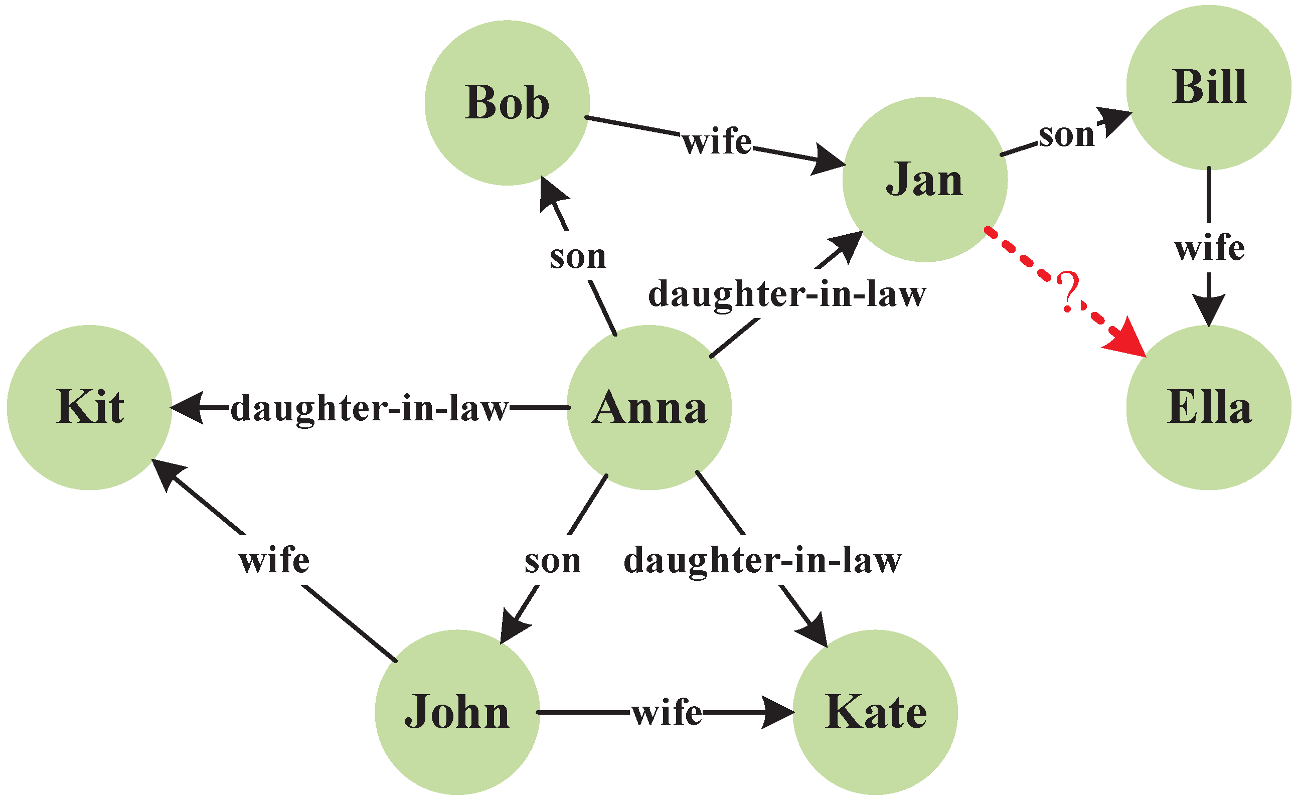
Many KGC methods use knowledge graph embedding (KGE) [10]. KGE represents entities and relations as continuous vectors and evaluates triples with a scoring function. Prior work has improved model expressiveness through TransE [11], ComplEx [12], and ConvE [13]. Other studies have developed graph encoders such as R-GCN [14], HRAN [15], and DisenKGAT [16]. These advances mainly improve how observed triples are encoded or scored. Positive training evidence still comes primarily from observed first-order triples, including in sampled noise contrastive estimation pipelines [17]. This design may underuse relational patterns contained in multi-hop paths. Figure 1 illustrates this issue. If person A is the wife of person B’s son, then A can be inferred as the daughter-in-law of B. Following the same rule, Ella can be inferred as the daughter-in-law of Jan because she is the wife of Jan’s son Bill. If training uses only the observed first-order triples around Ella, the daughter-in-law relation is unavailable as direct positive evidence. The challenge is not simply to find a multi-hop path. The method must determine whether the path supports the target relation and whether its grounding is reliable enough for training.

The existing rule-based approaches address different parts of this challenge. AnyBURL learns rules from sampled paths and uses rule confidence to rank candidate entities directly [18]. Neural LP learns differentiable rule structures for end-to-end query answering [19]. Rule-enhanced embedding methods instead use symbolic evidence during representation learning. For example, KnowAug iteratively mines rules, generates triples, and uses embeddings to validate them [20]. KG-Mixup creates synthetic triples for low-degree entity–relation pairs without using logic rules [21].

These methods leave a specific training problem unresolved. Rule confidence describes an entire rule, but individual groundings can differ in support, type compatibility, path consistency, and redundancy. Our research question is therefore: using only the training graph, how can we select reliable rule-derived triples and control their influence across different KGE scoring functions?

We address this question with target-relation-guided path sampling and candidate-level reliability weighting. The sampled paths induce Horn rules, which generate candidate triples. A reliability score combines rule-level and grounding-level evidence for each candidate. Selected candidates are then used as weighted positive samples alongside the original triples. The rules provide training evidence rather than final test-time rankings, so the method remains compatible with different KGE scoring functions.

We evaluate the method on WN18RR and FB15k-237 with five representative scoring functions. Matched Base/Aug comparisons measure the effect of adding the fixed weighted triples within the same training pipeline. Parameter sensitivity and ablation experiments examine when rule-derived evidence helps and when uncontrolled augmentation introduces noise.

The main contributions are:

1.

A model-agnostic interface transfers symbolic evidence into KGE training without replacing the embedding predictor with a rule reasoner.

2.

Target-relation-guided sampling and candidate-level reliability distinguish groundings by support, type validity, path consistency, and redundancy.

3.

Reliability-dependent weights control the contribution of each inferred triple to the embedding objective.

4.

Experiments with five scoring functions evaluate link prediction, parameter sensitivity, component ablation, and computational cost on WN18RR and FB15k-237.

2. Related Work

2.1. Knowledge Graph Completion

Knowledge graph completion aims to infer missing triples from observed triples. Embedding-based methods evaluate candidate triples through translation, semantic matching, or nonlinear scoring, as represented by TransE [11], DistMult [22], ComplEx [12], and ConvE [13]. Graph neural networks further incorporate neighborhood structure, including R-GCN [14], CompGCN [23], and LTE [24].

These methods mainly improve the scoring function or encoder. We instead use induced logic rules to generate positive training triples that can be shared across scoring functions.

2.2. Graph Sampling and Augmentation

Sampling supports representation learning by selecting local or random-walk contexts, as in Word2vec [25], LINE [26], DeepWalk [27], and node2vec [28]. Graph data augmentation modifies observed structures or generates synthetic instances [29,30,31,32,33]. For KGs, naive edge perturbation can introduce false facts because relations are typed and semantically constrained.

KGC-specific methods therefore add semantic constraints. KnowAug mines rules and filters generated triples with embeddings [20], whereas KG-Mixup generates synthetic triples for low-degree entity–relation pairs [21]. Our framework instead uses rule- and grounding-level evidence to select candidate triples and weight their contribution to KGE training.

2.3. Rule Learning and Reasoning

Rule learning provides an interpretable way to exploit multi-hop relational patterns in KGs. A rule such as $(r_1,r_2)\to r_3$ can explain why a missing relation is plausible through an observed path. Wu et al. [34] review major rule-learning paradigms over KGs and discuss their roles in link prediction, reasoning, and explanation. Recent transfer rule learning also studies how rules can be transferred across large KGs [35].

The existing methods use rules through different prediction interfaces. AnyBURL samples paths and directly ranks candidate entities with rule confidence [18], whereas Neural LP learns differentiable rule structures for end-to-end query answering [19]. Rule-based prediction and rule-guided augmentation therefore use symbolic evidence through different interfaces. Our method uses target-relation-guided sampling to generate candidates. It estimates the reliability of each grounding and transfers that estimate into a model-agnostic KGE objective.

3. Method

The method comprises three parts: formal definitions, rule-based augmentation, and reliability-weighted embedding training.

3.1. Preliminaries

3.1.1. Knowledge Graph

Formally, the KG $\mathcal{G}$ is

$$\mathcal{G}=(\mathcal{E},\mathcal{R},\mathcal{T})$$

(1)

where $\mathcal{E}=\{e_1,e_2,\dots ,e_{\left|\mathcal{E}\right|}\}$ and $\mathcal{R}=\{r_1,r_2,\dots ,r_{\left|\mathcal{R}\right|}\}$ are the entity and relation sets. The triple set is $\mathcal{T}\subseteq \mathcal{E}\times \mathcal{R}\times \mathcal{E}$. In a triple $(e_s,r,e_o)$, $e_s$ and $e_o$ are the subject and object entities, and r is their relation. The vectors ${\mathit{e}}_s,\mathit{r},{\mathit{e}}_o\in {\mathbb{R}}^d$ are their d-dimensional embeddings. The entity and relation embedding matrices are $\mathbf{E}\in {\mathbb{R}}^{\left|\mathcal{E}\right|\times d}$ and $\mathbf{R}\in {\mathbb{R}}^{\left|\mathcal{R}\right|\times d}$, respectively.

3.1.2. Task

Knowledge graph embedding (KGE) maps entities and relations to continuous vectors. Knowledge graph completion (KGC) uses these representations or other reasoning mechanisms to predict missing triples. Given an entity and a relation, the task ranks candidate entities for the missing subject or object. A scoring function $f(e_s,r,e_o)\in \mathbb{R}$ measures triple plausibility, and training assigns higher plausibility to observed triples than to corrupted triples.

3.1.3. Multi-Hop Neighbors

For an entity e, a k-hop neighbor is reachable by a relational walk of length k. First-order neighbors connect directly to e, whereas multi-hop neighbors require $k\ge 2$ edges. Here, multi-hop information denotes relational patterns carried by paths rather than by a single observed edge.

3.1.4. Logic Rules

Given two entities $e_1$ and $e_{n+1}$, a walk from $e_1$ to $e_{n+1}$ is recorded as

$$((e_1,r_1,e_2),(e_2,r_2,e_3),\cdots ,(e_n,r_n,e_{n+1})).$$

(2)

We formulate logic rules as first-order Horn clauses. Let $r_1,r_2,\dots ,r_n,\overline{r}\in \mathcal{R}$ be fixed relations. The sequence $(r_1,r_2,\dots ,r_n)$ denotes a relational path $((E_1,r_1,E_2),\dots ,(E_n,r_n,E_{n+1}))$. Each object variable is the subject variable of the next triple, and $E_1,\dots ,E_{n+1}$ denote entity variables.

A cyclic logic rule R is defined as

$$(r_1,r_2,\cdots ,r_n)\to \overline{r},$$

(3)

The subject of $r_1$ and the object of $r_n$ match the subject and object of $\overline{r}$, respectively. The relation sequence on the left is the rule body, and $\overline{r}$ on the right is the rule head. The rule is cyclic because the body and head form two paths between the same endpoint entities. Equation (2) gives a body path, whereas $(e_1,\overline{r},e_{n+1})$ gives the corresponding head path. Together they form a grounding, or instantiation, of the rule.

Figure 1 illustrates the rule

$$\left(\right(A,\mathit{son},B)\wedge (B,\mathit{wife},C\left)\right)\to (A,\mathit{daughter}\text{-}\mathit{in}\text{-}\mathit{law},C)$$

(4)

This rule states that, if C is the wife of A’s son B, then C is A’s daughter-in-law. The triples ((Anna, son, Bob), (Bob, wife, Jan)) form the body grounding. The triple (Anna, daughter-in-law, Jan) is the head grounding.

3.2. Rule-Based Augmentation

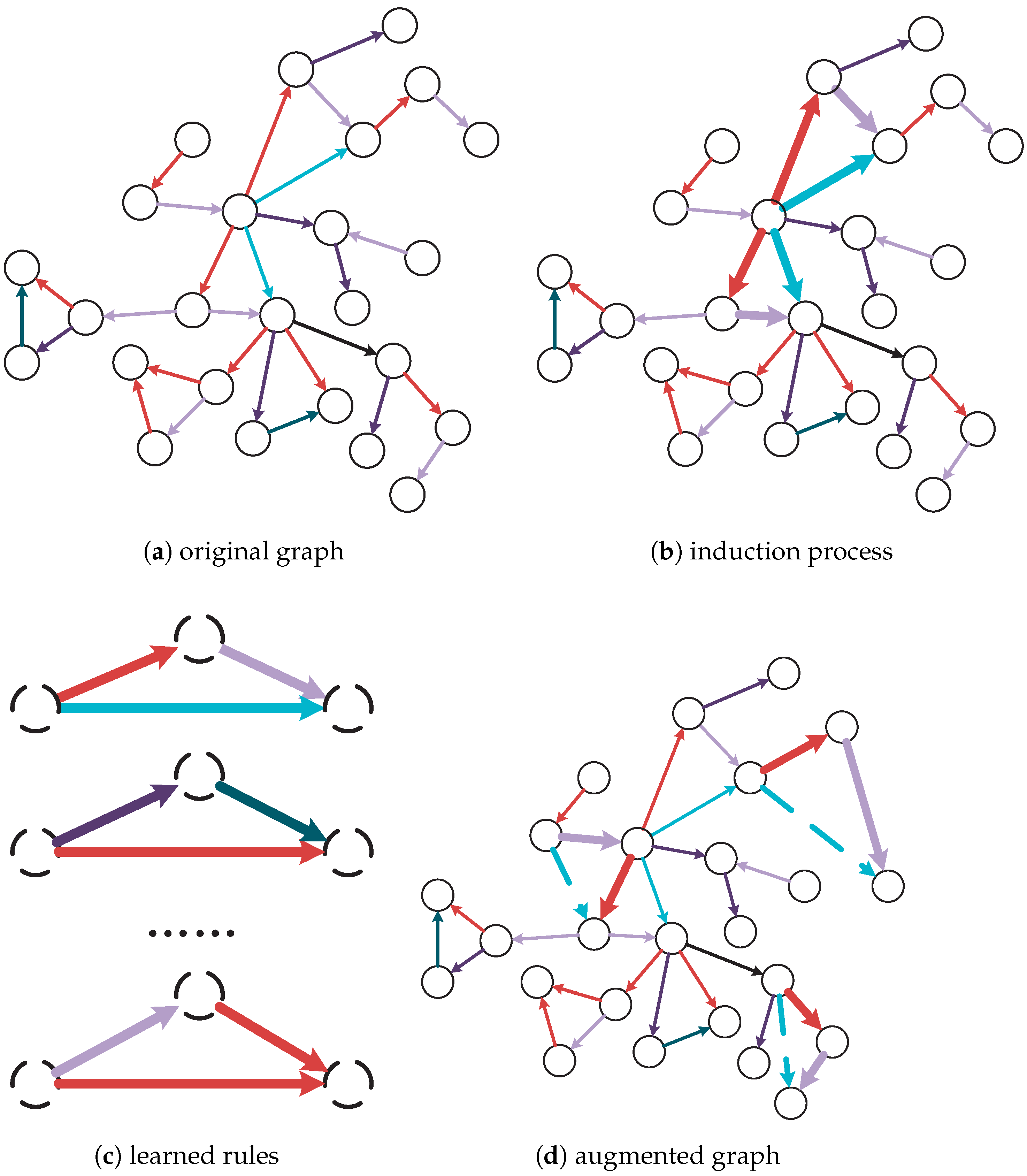
Multi-hop paths contain relational patterns that are absent from individual observed edges. We extract these patterns as logic rules and use their grounded conclusions as additional KGE training triples. For each benchmark, let ${\mathcal{T}}_{\mathrm{train}}$, ${\mathcal{T}}_{\mathrm{valid}}$, and ${\mathcal{T}}_{\mathrm{test}}$ denote the official data splits, and define the training graph as ${\mathcal{G}}_{\mathrm{train}}=(\mathcal{E},\mathcal{R},{\mathcal{T}}_{\mathrm{train}})$. All augmentation steps use only ${\mathcal{G}}_{\mathrm{train}}$. These steps include rule induction, guided-walk statistics, candidate generation, and reliability estimation. Candidates already in ${\mathcal{T}}_{\mathrm{train}}$ are removed, but validation and test membership is never queried. Any candidate matching a held-out fact is therefore inferred solely from the training graph. The offline procedure contains rule induction and rule inference (Figure 2).

Figure 2a shows the original training graph from which relational paths are sampled. Figure 2b illustrates how a closing body path is paired with an observed head triple during rule induction, and Figure 2c shows the resulting relation-level rules. Figure 2d shows how an induced rule is grounded on a non-closing path to produce a candidate for reliability filtering and weighted augmentation.

3.2.1. Rule Induction

Rule induction estimates which head relations are supported by each rule body. For a training triple $\tau =(e_1,\overline{r},e_{n+1})$, we sample paths from $e_1$ and retain those ending at $e_{n+1}$. Let $L_{\tau }$ be the number of retained body paths. Removing the entity identities yields $M_{\tau }$ distinct relation sequences ${\left\{(r_1^m,\dots ,r_n^m)\right\}}_{m=1}^{M_{\tau }}$. The observed relation $\overline{r}$ supplies the rule head. If $N_m$ is the number of groundings for body m, then $N_m\ge 1$ and ${\sum }_{m=1}^{M_{\tau }}{N}_m=L_{\tau }$. These counts are used to estimate the empirical support for each body–head pair.

However, if we set the rule length to n, exhaustive enumeration must traverse all length-n paths from the subject entity $e_1$ and retain those that end at the object entity $e_{n+1}$. For the complexity discussion, we define an untyped reachability projection

$$A_{i,j}^{\mathrm{reach}}=\mathbb{I}\left[\exists r\in \mathcal{R}:(e_i,r,e_j)\in {\mathcal{T}}_{\mathrm{train}}\right].$$

(5)

This binary projection is used only to describe reachable entity endpoints; it is not the graph representation used by the sampler. The sampler operates on the training-only relation-labeled adjacency list ${\mathcal{N}}_{\mathrm{rel}}^{\mathrm{train}}\left(e\right)=\{(r,e^{\prime })\mid (e,r,e^{\prime })\in {\mathcal{T}}_{\mathrm{train}}\}$, which retains distinct relations between the same pair of entities. Let $\omega ={\displaystyle \frac{1}{\left|\mathcal{E}\right|}}{\sum }_{e\in \mathcal{E}}\left|{\mathcal{N}}_{\mathrm{rel}}^{\mathrm{train}}\left(e\right)\right|$ denote the average number of outgoing relation-labeled transitions. Exhaustive relation-aware traversal therefore requires $O\left(\right|\mathcal{E}\left|{\omega }^n\right)$ transition expansions, which is expensive for large n.

Exhaustive traversal is costly and repeatedly discovers the same rule bodies. We therefore use guided random walks to sample body paths for each triple $\tau =(e_1,\overline{r},e_{n+1})$. Rather than assigning the same transition probability to every outgoing relation-labeled neighbor, the walker is biased toward informative and head-relevant relations while penalizing transitions into high-degree hub entities. For a candidate transition $(e_i,r_i,e_{i+1})$, define

$$q(e^{\prime },r^{\prime }\mid e_i,\overline{r})=aI\left(r^{\prime }\right)-b\log \mathrm{deg}\left(e^{\prime }\right)+c\mathrm{sim}(r^{\prime },\overline{r}).$$

(6)

The transition probability is the corresponding softmax over all relation-labeled outgoing transitions,

$$P(e_{i+1},r_i\mid e_i,\overline{r})={\displaystyle \frac{\exp q(e_{i+1},r_i\mid e_i,\overline{r})}{{\sum }_{(e^{\prime },r^{\prime })\in {\mathcal{N}}_{\mathrm{rel}}^{\mathrm{train}}\left(e_i\right)}\exp q(e^{\prime },r^{\prime }\mid e_i,\overline{r})}},$$

(7)

where $I\left(r^{\prime }\right)$ denotes relation informativeness, $\mathrm{deg}\left(e^{\prime }\right)$ is the out-degree of the next entity, $\mathrm{sim}(r^{\prime },\overline{r})$ measures the semantic or statistical relevance between the candidate body relation and the fixed target head relation, and a, b, and c are non-negative coefficients. Thus, the numerator and every denominator term use the same transition score and condition on the same target relation $\overline{r}$. In implementation, $I\left(r^{\prime }\right)$ and $\mathrm{sim}(r^{\prime },\overline{r})$ can be estimated from relation frequencies and co-occurrence statistics in the training KG. The guided and uniform samplers use the same walk budget, but the guided sampler favors paths that are more likely to support the target relation. The first step cannot move directly to the object entity, and later steps cannot immediately return to the preceding entity. The rule-body length is n, and each source triple permits at most N walks. Algorithm 1 gives the sampling procedure.

Algorithm 1 performs N independent guided random walks of length n for a given training triple. Each transition is sampled from the relation-labeled neighborhood of the current terminal entity ${\overline{e}}_t$, so the subject of every new edge equals the object of the preceding edge and ${\mathcal{L}}_{\mathrm{total}}$ remains a continuous path. Only walks satisfying $\mathrm{len}\left({\mathcal{L}}_{\mathrm{total}}\right)=n$ are retained: walks ending at $e_{n+1}$ enter $\mathcal{L}$ as rule-induction evidence, and the other complete walks enter ${\mathcal{L}}_{\mathrm{other}}$ for candidate generation. The first step does not directly move to $e_{n+1}$, and later steps avoid immediately returning to the previous entity, which reduces trivial one-edge explanations and short backtracking loops. After sampling for $\tau =(e_1,\overline{r},e_{n+1})$, the relation sequences of walks ending at $e_{n+1}$ define the rule bodies, and $\overline{r}$ defines the head. The following empirical distributions aggregate these observations directly.

Algorithm 1 Path sampling

Input:  training triple $\tau =(e_1,\overline{r},e_{n+1})$; length n; maximum number of walks N; training adjacency list $L_{\mathrm{train}}$ Output:  complete paths ending at $e_{n+1}$, $\mathcal{L}$; complete paths ending elsewhere, ${\mathcal{L}}_{other}$   1: $\mathcal{L}$ ← ∅;                   ▹ list to store all walks that end in $e_{n+1}$;   2: ${\mathcal{L}}_{other}$ ← ∅;               ▹ list to store all walks that do not end in $e_{n+1}$   3: $iter=1$   4: while  $iter\le N$  do   5:     ${\mathcal{L}}_{total}$ ← ∅;   6:     ${\mathcal{L}}_{pre}$ ← ∅;   7:     for $t=1,2,,n$ do   8:         if $t=1$ then   9:              sample $(r_1,{\overline{e}}_2)$ from ${\mathcal{N}}_{\mathrm{rel}}^{\mathrm{train}}\left(e_1\right)$ according to Equation (7); 10:            if ${\overline{e}}_2$ ≠ $e_{n+1}$ then 11:                ${\mathcal{L}}_{total}=\left((e_1,r_1,{\overline{e}}_2)\right)$; 12:            else 13:                break; 14:            end if 15:         else 16:            get the last triple $({\overline{e}}_{t-1},r_{t-1},{\overline{e}}_t)$ of ${\mathcal{L}}_{pre}$; 17:            sample $(r_t,{\overline{e}}_{t+1})$ from ${\mathcal{N}}_{\mathrm{rel}}^{\mathrm{train}}\left({\overline{e}}_t\right)$ according to Equation (7); 18:            if ${\overline{e}}_{t+1}$ ≠ ${\overline{e}}_{t-1}$ then 19:                ${\mathcal{L}}_{total}={\mathcal{L}}_{total}\bigcup ({\overline{e}}_t,r_t,{\overline{e}}_{t+1})$; 20:            else 21:                break; 22:            end if 23:         end if 24:         ${\mathcal{L}}_{pre}\leftarrow {\mathcal{L}}_{total}$; 25:     end for 26:     $iter=iter+1$ 27:     if len$({\mathcal{L}}_{total})==n$ then 28:         if $e_{n+1}={\overline{e}}_{n+1}$ then 29:            add ${\mathcal{L}}_{total}$ into $\mathcal{L}$; 30:         else 31:            add ${\mathcal{L}}_{total}$ into ${\mathcal{L}}_{other}$; 32:         end if 33:     end if 34: end while 35: return $\mathcal{L}$, ${\mathcal{L}}_{other}$

We apply the path sampling algorithm to every source triple and estimate rule statistics only from sampled paths that close at the source triple’s object entity. For $\tau =(e_1,\overline{r},e_{n+1})$, let $N_{\tau }\left(r_b\right)$ be the number of closed sampled paths with relation sequence $r_b$, and let $L_{\tau }={\sum }_{r_b}{N}_{\tau }\left(r_b\right)$ be the total number of closed sampled paths. For $L_{\tau }>0$, we define the joint empirical distribution directly as

$$\widehat{P}(R_b=r_b,R_h=r_h\mid T=\tau )={\displaystyle \frac{N_{\tau }\left(r_b\right)}{L_{\tau }}}\mathbb{I}[r_h=\overline{r}].$$

(8)

This definition does not factor the joint distribution and therefore does not assume that $R_b$ and $R_h$ are conditionally independent given $\tau$. Its conditional marginals are

$$\begin{array}{cc}\hfill \widehat{P}(R_b=r_b\mid T=\tau )& ={\displaystyle \frac{N_{\tau }\left(r_b\right)}{L_{\tau }}},\hfill \\ \hfill \widehat{P}(R_h=r_h\mid T=\tau )& =\mathbb{I}[r_h=\overline{r}].\hfill \end{array}$$

(9)

If $L_{\tau }=0$, the source triple contributes no rule statistic. Let ${\mathcal{T}}_{\mathrm{train},+}=\{\tau \in {\mathcal{T}}_{\mathrm{train}}\mid L_{\tau }>0\}$, and assign equal mass to its eligible source triples. The global joint and marginal empirical distributions are then obtained by aggregation:

$$\begin{array}{cc}\hfill \widehat{P}(R_b=r_b,R_h=r_h)& ={\displaystyle \frac{1}{|{\mathcal{T}}_{\mathrm{train},+}|}}\sum _{\tau \in {\mathcal{T}}_{\mathrm{train},+}}\widehat{P}(R_b=r_b,R_h=r_h\mid T=\tau ),\hfill \\ \hfill \widehat{P}(R_b=r_b)& =\sum _{r_h\in \mathcal{R}}\widehat{P}(R_b=r_b,R_h=r_h).\hfill \end{array}$$

(10)

The empirical reliability of a rule body for a head relation is

$$\widehat{P}(R_h=r_h\mid R_b=r_b)={\displaystyle \frac{\widehat{P}(R_b=r_b,R_h=r_h)}{\widehat{P}(R_b=r_b)}}.$$

(11)

We retain rules whose empirical reliability exceeds the threshold $\mathcal{M}$ and store $\mathcal{S}=\{(r_b\to r_h,\widehat{P}(R_h=r_h\mid R_b=r_b))\}$. Algorithm 2 summarizes rule induction.

Algorithm 2 Rule induction

Input:  maximum number of walks N; length n; training graph ${\mathcal{G}}_{\mathrm{train}}=(\mathcal{E},\mathcal{R},{\mathcal{T}}_{\mathrm{train}})$; rule-retention threshold $\mathcal{M}$; training adjacency list $L_{\mathrm{train}}$; Output:  empirical distributions $\widehat{P}(R_b,R_h)$, $\widehat{P}\left(R_b\right)$, and $\widehat{P}\left(R_h\right|R_b)$; retained rule set $\mathcal{S}$;   1: $\mathcal{S}$ ← ∅;   2: for $\tau =(e_1,\overline{r},e_{n+1})$ in ${\mathcal{T}}_{\mathrm{train}}$ do   3:     $(\mathcal{L},{\mathcal{L}}_{other})$ ← path sampling($e_1,\overline{r},e_{n+1}$, n, N, $L_{\mathrm{train}}$);   4:     for $path$ in $\mathcal{L}$ do                  ▹ abstract rule body and rule head from walk   5:         abstract rule body $r_b=(r_1,r_2,\dots ,r_n)$ from $path$;   6:         abstract rule head $r_h=\overline{r}$;   7:         update the closed-path counts $N_{\tau }\left(r_b\right)$ and $L_{\tau }$;   8:     end for   9: end for 10: calculate the empirical distributions using Equations (8)–(11); 11: for each observed pair $(r_b,r_h)$ do 12:     if $\widehat{P}(R_h=r_h\mid R_b=r_b)\ge \mathcal{M}$ then 13:         $\mathcal{S}\leftarrow \mathcal{S}\cup \left\{(r_b\to r_h,\widehat{P}(R_h=r_h\mid R_b=r_b))\right\}$; 14:     end if 15: end for 16: return $\widehat{P}(R_b,R_h)$, $\widehat{P}\left(R_b\right)$, $\widehat{P}\left(R_h\right|R_b)$, and $\mathcal{S}$

3.2.2. Rule Inference

Rule inference is also restricted to ${\mathcal{G}}_{\mathrm{train}}$. For each source triple $\tau =(e_1,\overline{r},e_{n+1})\in {\mathcal{T}}_{\mathrm{train}}$, we use the complete non-closing paths in ${\mathcal{L}}_{\mathrm{other}}$ to generate candidates. For each such path, we first extract its relation sequence $r_b$ and then retrieve every retained rule $(r_b\to r_h,\widehat{P})\in \mathcal{S}$ whose body matches that sequence. Only after $r_h$ has been instantiated do we construct ${\tau }^{\prime }=(e_1,r_h,e_{\mathrm{end}})$ and discard it if ${\tau }^{\prime }\in {\mathcal{T}}_{\mathrm{train}}$. We aggregate all the derivations of each remaining candidate before computing reliability. The deduplicated candidates are then ranked, and at most K are retained for each source triple. The marginal-frequency-normalized ratios used in the previous formulation are association quantities rather than bounded probabilities, and their product has no valid probabilistic interpretation because the body marginal cancels and the result is rescaled by the head marginal. We therefore do not use that product for candidate ranking or training. Instead, the closed-path conditional in Equation (11) supplies the rule-level statistic, and the following candidate-level reliability score combines the evidence associated with each generated grounding:

$$\begin{array}{cc}\hfill {\mathrm{Conf}}_{aug}\left({\tau }^{\prime }\right)=& {\rho }_1{\mathrm{Conf}}_{smooth}(r_b\to r_h)+{\rho }_2{\mathrm{support}}_{norm}(r_b\to r_h)\hfill \\ \hfill & +{\rho }_3\mathrm{type}\text{\_}\mathrm{valid}\left({\tau }^{\prime }\right)+{\rho }_4\mathrm{path}\text{\_}\mathrm{consistency}\left({\tau }^{\prime }\right)-{\rho }_5\mathrm{redundancy}\left({\tau }^{\prime }\right),\hfill \end{array}$$

(12)

where ${\tau }^{\prime }=(e_1,r_h,{\overline{e}}_{n+1})$ denotes a candidate augmented triple. The five coefficients respectively weight smoothed rule reliability, normalized support, type validity, path consistency, and redundancy. They are fixed uniformly as ${\rho }_1={\rho }_2={\rho }_3={\rho }_4={\rho }_5=0.2$, shared across datasets and scoring models, and not optimized on the validation set. The smoothed rule reliability is defined as

$${\mathrm{Conf}}_{smooth}(r_b\to r_h)={\displaystyle \frac{N(r_b,r_h)}{N\left(r_b\right)+3}},$$

(13)

where $N(r_b,r_h)$ is the number of closed sampled paths in which body $r_b$ supports head $r_h$, and $N\left(r_b\right)$ is the number of closed sampled paths containing the body. The denominator-additive smoothing constant is fixed at $p_c=3$ for all datasets and scoring models and is not tuned on the validation set. It imposes a conservative three-count penalty on low-support rules, while its relative influence decreases as $N\left(r_b\right)$ grows. These counts are statistics of the closed sampled paths rather than exhaustive counts of all possible body groundings. To make each remaining term explicit, let $\mathcal{D}\left({\tau }^{\prime }\right)$ denote the set of derivations that produce the same candidate triple ${\tau }^{\prime }=(h,r,t)$. Each derivation is a pair $(r_b,p)$, where $r_b$ is the rule body and p is a sampled path whose terminal entity is t. Let $\mathcal{B}\left({\tau }^{\prime }\right)=\{r_b\mid (r_b,p)\in \mathcal{D}\left({\tau }^{\prime }\right)\}$ be the set of distinct rule bodies supporting ${\tau }^{\prime }$. The normalized support of a rule is

$${\mathrm{support}}_{norm}(r_b\to r_h)={\displaystyle \frac{\log (1+N(r_b,r_h))}{\log (1+{\max }_{(r_b^{\prime },r_h^{\prime })\in \mathcal{S}}N(r_b^{\prime },r_h^{\prime }))}}.$$

(14)

The type-validity term is estimated from the empirical domain and range of each relation:

$$\mathrm{Domain}\left(r\right)=\{h\mid \exists t,(h,r,t)\in {\mathcal{T}}_{\mathrm{train}}\},\mathrm{Range}\left(r\right)=\{t\mid \exists h,(h,r,t)\in {\mathcal{T}}_{\mathrm{train}}\},$$

(15)

$$\mathrm{type}\text{\_}\mathrm{valid}(h,r,t)=\mathbb{I}[h\in \mathrm{Domain}(r\left)\right]·\mathbb{I}[t\in \mathrm{Range}(r\left)\right].$$

(16)

The path-consistency term rewards candidate triples that are repeatedly supported by sampled paths:

$$\mathrm{path}\text{\_}\mathrm{consistency}\left({\tau }^{\prime }\right)={\displaystyle \frac{\log (1+|\mathcal{D}\left({\tau }^{\prime }\right)\left|\right)}{\log (1+{\max }_{\tilde{\tau }\in {\mathcal{T}}_A}|\mathcal{D}\left(\tilde{\tau }\right)\left|\right)}}.$$

(17)

Finally, the redundancy term penalizes cases where many derivations collapse to the same rule body and therefore provide little independent evidence:

$$\mathrm{redundancy}\left({\tau }^{\prime }\right)=1-{\displaystyle \frac{\left|\mathcal{B}\right({\tau }^{\prime }\left)\right|}{\left|\mathcal{D}\right({\tau }^{\prime }\left)\right|}}.$$

(18)

All five component terms in Equation (12) are bounded in $[0,1]$. Because a common positive scaling of ${\rho }_1,\dots ,{\rho }_5$ cancels under the subsequent min–max transformation, the normalized equal-weight setting above is equivalent to the implementation’s fixed equal coefficients. For each source triple, candidates are deduplicated and sorted by ${\mathrm{Conf}}_{aug}\left({\tau }^{\prime }\right)$, and at most the top $K=3$ candidates are retained. Algorithm 3 gives the inference procedure.

Algorithm 3 Rule inference

Input:  length n; maximum number of walks N; rule set $\mathcal{S}=\left\{(r_b\to r_h,\widehat{P}(R_h=r_h\mid R_b=r_b))\right\}$; training graph ${\mathcal{G}}_{\mathrm{train}}=(\mathcal{E},\mathcal{R},{\mathcal{T}}_{\mathrm{train}})$; training adjacency list $L_{\mathrm{train}}$; per-source cutoff $K=3$; Output:  weighted augmented triple set ${\mathcal{T}}_A$   1: ${\mathcal{T}}_A\leftarrow \varnothing$;   2: for $\tau =(e_1,\overline{r},e_{n+1})$ in ${\mathcal{T}}_{\mathrm{train}}$ do   3:     $(\mathcal{L},{\mathcal{L}}_{other})\leftarrow$ path sampling($e_1,\overline{r},e_{n+1}$, n, N, $L_{\mathrm{train}}$);   4:     initialize an empty candidate map ${\mathcal{C}}_{\tau }$;   5:     for $path$ in ${\mathcal{L}}_{other}$ do   6:         extract terminal entity $e_{\mathrm{end}}$ and relation sequence $r_b$ from $path$;   7:         for each retained rule $(r_b\to r_h,\widehat{P})\in \mathcal{S}$ matching $r_b$ do   8:            instantiate ${\tau }^{\prime }=(e_1,r_h,e_{\mathrm{end}})$;   9:            if ${\tau }^{\prime }\notin {\mathcal{T}}_{\mathrm{train}}$ then 10:                add derivation $(r_b,path)$ to $\mathcal{D}\left({\tau }^{\prime }\right)$ in ${\mathcal{C}}_{\tau }$; 11:            end if 12:         end for 13:     end for 14:     for each deduplicated candidate ${\tau }^{\prime }$ in ${\mathcal{C}}_{\tau }$ do 15:         calculate ${\mathrm{Conf}}_{aug}\left({\tau }^{\prime }\right)$ from all derivations $\mathcal{D}\left({\tau }^{\prime }\right)$; 16:     end for 17:     add at most the top K candidates in ${\mathcal{C}}_{\tau }$ to ${\mathcal{T}}_A$; 18: end for 19: return  ${\mathcal{T}}_A$

3.3. Encoder and Objective

Entity neighborhoods contain relation-specific information. We use a modified graph attention network to aggregate this information while distinguishing relation types.

Let ${\mathbf{e}}_u^0$ and ${\mathbf{e}}_r^0$ be the initial embeddings of entity u and relation r, respectively. Superscript l denotes a layer index. At layer l, the relation-specific message is

$$m^l(u,r)={\mathbf{e}}_u^{l-1}\circ {\theta }_r\circ {\mathbf{e}}_r^{l-1},$$

(19)

where ∘ denotes element-wise multiplication, ${\theta }_r\in {\mathbb{R}}^d$ denotes the relation-aware projection vector, and l denotes the layer of our graph attention network. Next, we calculate an unnormalized score and normalize it over the relation-labeled neighborhood:

$$s^l(u,r,v)=\mathrm{LeakyReLU}\left({\left(m^l(u,r)\right)}^T{m}^l(v,r)\right),$$

(20)

$${\alpha }^l(u,r,v)={\displaystyle \frac{\exp \left(s^l(u,r,v)\right)}{{\sum }_{(v^{\prime },r^{\prime })\in {\mathcal{N}}_u}\exp \left(s^l(u,r^{\prime },v^{\prime })\right)}}.$$

(21)

Here, ${\mathcal{N}}_u$ is the set of relation-labeled neighbors $(v,r)$ of entity u, including its self-loop. The implementation uses this neighborhood-wise exponentiated softmax. Following the common GAT setting, the LeakyReLU negative slope is 0.2:

$$\mathrm{LeakyReLU}\left(x\right)=\left\{\begin{array}{cc}x,\hfill & \mathrm{if}x\ge 0,\hfill \\ 0.2x,\hfill & \mathrm{if}x<0.\hfill \end{array}\right.$$

(22)

The updated embedding of entity u is

$${\mathbf{e}}_u^l=\sum _{(v,r)\in {\mathcal{N}}_u}{\alpha }^l(u,r,v)·m^l(v,r).$$

(23)

Relations are updated by a layer-specific linear transformation:

$${\mathbf{e}}_r^l=W^l·{\mathbf{e}}_r^{l-1}.$$

(24)

We use the last-layer embeddings to calculate a decoder score $f_{\theta }\left(\tau \right)$ for a triple $\tau =(e_s,r,e_o)$. To give every decoder the same orientation, we define a plausibility logit

$$z_{\theta }\left(\tau \right)=\left\{\begin{array}{cc}-f_{\theta }\left(\tau \right),\hfill & \mathrm{for}\mathrm{distance}\text{-}\mathrm{based}\mathrm{decoders}\mathrm{such}\mathrm{as}\mathrm{TransE},\hfill \\ f_{\theta }\left(\tau \right),\hfill & \mathrm{for}\mathrm{similarity}\text{-}\mathrm{based}\mathrm{decoders}.\hfill \end{array}\right.$$

(25)

Thus, a larger $z_{\theta }\left(\tau \right)$ always indicates a more plausible triple. The predicted probability is $p_{\theta }\left(\tau \right)=\sigma \left(z_{\theta }\left(\tau \right)\right)$, where $\sigma \left(x\right)={(1+\exp (-x))}^{-1}$. For a graph $\mathcal{G}$, binary cross-entropy is applied to this bounded probability,

$$L_{\mathcal{G}}=-\sum _{(e_s,r,e_o)\in {\mathcal{T}}_{\mathcal{G}}^{+}\cup {\mathcal{T}}_{\mathcal{G}}^{-}}\left[y\log \sigma \left(z_{\theta }\left(\tau \right)\right)+(1-y)\log \left(1-\sigma \left(z_{\theta }\left(\tau \right)\right)\right)\right],$$

(26)

where ${\mathcal{T}}_{\mathcal{G}}^{+}$ denotes the positive samples and ${\mathcal{T}}_{\mathcal{G}}^{-}$ denotes the negative samples. The label y is defined as

$$y=\left\{\begin{array}{cc}1,\hfill & \mathrm{if}(e_s,r,e_o)\in {\mathcal{T}}_{\mathcal{G}}^{+},\hfill \\ 0,\hfill & \mathrm{if}(e_s,r,e_o)\in {\mathcal{T}}_{\mathcal{G}}^{-}.\hfill \end{array}\right.$$

(27)

For the original graph, observed triples are treated as reliable positive samples and optimized with $L_{{\mathcal{G}}_O}$. For the augmented graph, the generated triples have different degrees of reliability, so we do not assign identical positive weight to all of them. Let $\mathcal{C}$ be the global set of generated candidates in one augmentation run before per-source top-K selection, let $s_{\tau }={\mathrm{Conf}}_{aug}\left(\tau \right)$, and define

$$s_{\min }=\underset{\tau \in \mathcal{C}}{\min }{s}_{\tau },s_{\max }=\underset{\tau \in \mathcal{C}}{\max }{s}_{\tau }.$$

(28)

The global candidate pool contains distinct reliability scores in the reported runs, so $s_{\max }>s_{\min }$. For each retained augmented triple $\tau \in {\mathcal{T}}_A$, its bounded training weight is

$$w_{\tau }={\displaystyle \frac{s_{\tau }-s_{\min }}{s_{\max }-s_{\min }}}.$$

(29)

This min–max transformation preserves the candidate ordering and maps the reliability scores to $[0,1]$; it is used as a training-weight transformation rather than interpreted as probabilistic calibration. Let $\ell \left(\tau \right)$ denote the binary cross-entropy term for an augmented triple and its sampled negatives. The augmented loss is then defined as

$$L_{{\mathcal{G}}_A}=\sum _{\tau \in {\mathcal{T}}_A}{w}_{\tau }·\ell \left(\tau \right).$$

(30)

The total loss combines binary cross-entropy on the original graph ${\mathcal{G}}_O$ with the reliability-weighted augmented loss,

$$L=L_{{\mathcal{G}}_O}+\lambda \sum _{\tau \in {\mathcal{T}}_A}{w}_{\tau }·\ell \left(\tau \right),$$

(31)

where $\lambda$ controls the contribution of augmented triples.

4. Experiments

We evaluate link-prediction accuracy, parameter sensitivity, component contributions, and computational cost.

4.1. Setup

4.1.1. Datasets

We use the WN18RR and FB15k-237 benchmarks [15]. Both provide official training, validation, and test splits (

Table 1. Dataset statistics.

Datasets		WN18RR	FB15k-237
# Entities		40,493	14,541
# Relations		11	237
# Edges	Train	86,835	272,115
	Valid	3034	17,535
	Test	3134	20,466
	Total	93,003	310,116
# Mean Degree		2.12	18.71

).

• WN18RR [15] is derived from WN18 [11] and ultimately from WordNet [7]. Its relations describe lexical links such as hypernymy and meronymy.
• FB15k-237 [15] is derived from FB15k [36] and Freebase [6]. It covers entities and relations from domains including people, organizations, locations, culture, and media.

4.1.2. Augmentation Protocol

For each dataset, rule induction and candidate generation run once as offline preprocessing with augmentation seed 42. The procedure applies rule induction to ${\mathcal{T}}_{\mathrm{train}}$, generates and deduplicates candidates, and retains the top K candidates in ${\mathcal{T}}_A$. KGE training then uses the fixed augmented set. The validation split is used only for KGE early stopping and model selection, and neither ${\mathcal{T}}_{\mathrm{valid}}$ nor ${\mathcal{T}}_{\mathrm{test}}$ is accessed during rule induction, candidate generation, reliability computation, deduplication, or top-K selection. After reliability filtering, deduplication, and per-source top-K selection, the fixed augmented sets contain 987 weighted triples for WN18RR and 14,389 for FB15k-237. They are generated before KGE optimization, are not regenerated between epochs, and are reused across all scoring models and KGE runs with seeds 41, 42, and 43. All controlled Base/Aug comparisons use the same graph-attention encoder, scoring-function decoder, negative-sampling strategy, optimizer, early-stopping criterion, and KGE training seeds. Within each pair, the only experimental factor is whether the fixed weighted augmentation set is included in the training objective. The resulting mean and standard deviation therefore quantify KGE training variability for a fixed augmentation set; they do not quantify uncertainty across rule-sampling seeds.

4.1.3. Baselines

We evaluate the augmentation method with five representative KGE decoders: a translation model, semantic-matching models, and neural scoring models.

• TransE: TransE [11] uses the translation distance

  $$f(e_s,r,e_o)={\parallel {\mathbf{e}}_s+\mathbf{r}-{\mathbf{e}}_o\parallel }_2,$$

  where ${\parallel ·\parallel }_2$ is the Euclidean norm.
• DistMult: DistMult [22] uses the bilinear score

  $$f(e_s,r,e_o)=\langle {\mathbf{e}}_s,\mathrm{diag}\left(\mathbf{r}\right),{\mathbf{e}}_o\rangle ,$$

  where $\langle a,b,c\rangle ={\sum }_{i=1}^d{a}_i{b}_i{c}_i$ and $\mathrm{diag}\left(\mathbf{r}\right)$ is a diagonal relation matrix.
• ComplEx: ComplEx [12] extends bilinear scoring to complex embeddings, allowing both symmetric and antisymmetric relations,

  $$\begin{array}{cc}\hfill f(e_s,r,e_o)& =\mathrm{R}({\mathit{e}}_s⨂\mathit{r}⨂\overline{{\mathit{e}}_o})\hfill \\ & =〈\mathrm{R}\left({\mathit{e}}_s\right),\mathrm{R}\left(\mathit{r}\right),\mathrm{R}\left({\mathit{e}}_o\right)〉+〈\mathrm{R}\left({\mathit{e}}_s\right),\mathrm{R}\left(\mathit{r}\right),\mathrm{I}\left({\mathit{e}}_o\right)〉\hfill \\ & +〈\mathrm{R}\left({\mathit{e}}_s\right),\mathrm{I}\left(\mathit{r}\right),\mathrm{I}\left({\mathit{e}}_o\right)〉-〈\mathrm{I}\left({\mathit{e}}_s\right),\mathrm{I}\left(\mathit{r}\right),\mathrm{R}\left({\mathit{e}}_o\right)〉,\hfill \end{array}$$

  where $\mathrm{R}\left(v\right)$ and $\mathrm{I}\left(v\right)$ denote the real and imaginary components.
• ConvE: ConvE [13] applies a multilayer convolutional network to entity and relation embeddings,

  $$f(e_s,r,e_o)=g\left(\mathrm{vec}([{\mathbf{e}}_s;\mathbf{r}]\star )\mathbf{W}\right){\mathbf{e}}_o,$$

  where ⋆ is convolution, $\mathsf{\Omega }$ is the convolutional kernel, W is a parameter matrix, and vec flattens its input.
• AutoBLM: AutoBLM [37] uses neural architecture search to select a bilinear scoring function.

For the controlled comparison, we use the encoder in Section 3.3 with each of the five scoring-function decoders. We denote a model trained only on the original training triples as Base and the matched model trained with the fixed weighted augmentation set as Aug.

4.1.4. Metrics

The AnyBURL MRR values in

Table 2. Results of link prediction by MR, MRR, and Hits@k on WN18RR and FB15k-237. The KnowAug and KG-Mixup values are from their original papers. A double dash denotes an unreported metric or dataset. Where the bold indicate the best result underlined indicates the second best result.

Methods		WN18RR					FB15k-237
		MR	MRR	Hits			MR	MRR	Hits
				@1	@3	@10			@1	@3	@10
Embeddings	TransE [11]	2879	0.198	0.047	0.306	0.476	189	0.329	0.240	0.364	0.507
	DistMult [22]	6024	0.434	0.402	0.451	0.498	269	0.331	0.244	0.363	0.504
	ConvE [13]	2520	0.476	0.447	0.492	0.540	180	0.358	0.266	0.393	0.545
	ComplEx [12]	4303	0.454	0.418	0.469	0.526	250	0.342	0.252	0.376	0.522
	AutoBLM [37]	3198	0.461	0.423	0.476	0.536	171	0.362	0.269	0.399	0.550
GNNs	CompGCN+TransE [23]	3182	0.206	0.064	0.281	0.502	205	0.335	0.247	0.369	0.511
	CompGCN+DistMult [23]	4559	0.430	0.395	0.439	0.513	200	0.342	0.252	0.372	0.520
	CompGCN+ConvE [23]	3065	0.469	0.433	0.480	0.543	245	0.351	0.254	0.386	0.535
	LTE+TransE [24]	3290	0.211	0.022	0.362	0.521	182	0.334	0.241	0.347	0.519
	LTE+DistMult [24]	4485	0.437	0.403	0.447	0.517	238	0.335	0.246	0.360	0.517
	LTE+ConvE [24]	3434	0.472	0.436	0.485	0.544	249	0.352	0.262	0.385	0.533
Rules	AnyBURL [18]	–	≥0.470	0.441	–	0.552	–	≥0.310	0.233	–	0.486
	RuleN [38]	–	–	0.427	–	0.536	–	–	0.182	–	0.420
	RLvLR [39]	–	–	–	–	–	–	0.240	–	–	0.393
Augmentation Baselines	KnowAug (ComplEx) [20]	–	0.453	0.414	–	0.535	–	0.331	0.239	–	0.516
	KG-Mixup (ConvE) [21]	–	–	–	–	–	–	0.343	0.250	–	0.531
Augmentations (Ours)	TransE–Aug	2706	0.208	0.043	0.316	0.489	177	0.331	0.242	0.375	0.525
	DistMult–Aug	5879	0.435	0.412	0.469	0.510	232	0.334	0.247	0.369	0.517
	ConvE–Aug	2032	0.491	0.457	0.503	0.553	173	0.362	0.271	0.401	0.552
	ComplEx–Aug	3042	0.461	0.423	0.472	0.541	245	0.346	0.256	0.379	0.527
	AutoBLM–Aug	2441	0.481	0.451	0.496	0.545	156	0.372	0.278	0.412	0.557

are lower bounds because its original evaluation computes top-k rather than complete rankings.

We follow the standard filtered link-prediction protocol used in [14,15,16]. For each test query, corrupted candidates that occur in the known-positive set $\mathcal{F}={\mathcal{T}}_{\mathrm{train}}\cup {\mathcal{T}}_{\mathrm{valid}}\cup {\mathcal{T}}_{\mathrm{test}}\cup {\mathcal{T}}_A$ are removed except for the target test triple itself. Including ${\mathcal{T}}_A$ in $\mathcal{F}$ prevents another rule-derived positive from being counted as a negative during evaluation; it does not expose held-out triples to the augmentation pipeline.

We report mean rank (MR), mean reciprocal rank (MRR), and Hits@k for $k\in \{1,3,10\}$,

$$\left\{\begin{array}{c}\mathrm{MR}\text{:}{\displaystyle \frac{1}{2|{\mathcal{T}}_{\mathrm{test}}|}}\sum _{x_i\in {\mathcal{T}}_{\mathrm{test}}}({\mathrm{rank}}_i^s+{\mathrm{rank}}_i^o)\hfill \\ \mathrm{MRR}\text{:}{\displaystyle \frac{1}{2|{\mathcal{T}}_{\mathrm{test}}|}}\sum _{x_i\in {\mathcal{T}}_{\mathrm{test}}}({\displaystyle \frac{1}{{\mathrm{rank}}_i^s}}+{\displaystyle \frac{1}{{\mathrm{rank}}_i^o}})\hfill \\ \mathrm{Hits}\text{@}k:{\displaystyle \frac{1}{2|{\mathcal{T}}_{\mathrm{test}}|}}\sum _{x_i\in {\mathcal{T}}_{\mathrm{test}}}I[{\mathrm{rank}}_i^s\le k]+I[{\mathrm{rank}}_i^o\le k]\hfill \end{array}\right.,$$

(32)

where ${\mathrm{rank}}_i^s$ and ${\mathrm{rank}}_i^o$ are

$$\left\{\begin{array}{c}{\mathrm{rank}}_i^s=(\sum _{{\widetilde{x_i}}^s\notin \mathcal{F}}I[z_{\theta }(x_i)<z_{\theta }({\widetilde{x_i}}^s)])+1\hfill \\ {\mathrm{rank}}_i^o=(\sum _{{\widetilde{x_i}}^o\notin \mathcal{F}}I[z_{\theta }(x_i)<z_{\theta }({\widetilde{x_i}}^o)])+1\hfill \end{array}\right..$$

(33)

Here, $x_i$ is the ith test triple, while ${\widetilde{x_i}}^s$ and ${\widetilde{x_i}}^o$ replace its subject and object, respectively. The indicator $I\left(P\right)$ equals 1 when P is true and 0 otherwise. A larger $z_{\theta }$ always denotes a more plausible triple. Lower MR and higher MRR or Hits@k indicate better performance.

4.1.5. Implementation

The rule-body lengths are set to $n\in \{2,3\}$, the rule-retention threshold is $\mathcal{M}=0.6$, at most the top $K=3$ deduplicated candidates are retained for each source triple, and the maximum number of random walks per source triple is $N=2000$. The smoothing constant is fixed at $p_c=3$, and the candidate-reliability coefficients are fixed at ${\rho }_1=\cdots ={\rho }_5=0.2$; these settings are shared across datasets and scoring models and are not tuned on the validation set. For embedding learning, the learning rate is 0.001, the batch size is 512, the dropout rate is 0.3, the graph attention network contains one layer, the embedding dimension is 400, and early stopping is applied with a patience of 50 epochs. The offline augmentation stage uses seed 42, and KGE training uses seeds 41, 42, and 43. After reliability filtering, deduplication, and top-K selection, 987 and 14,389 triples, respectively, are retained as weighted positive training samples. The method is implemented in PyTorch 1.13.0 and run on an NVIDIA GTX 1080 Ti GPU. The available timing records were collected under a common protocol, but they do not preserve a physical time unit or memory-profiler metadata. We therefore report only within-dataset time ratios normalized by the corresponding Base KGE run and do not make absolute runtime, memory, or cross-platform scalability claims.

4.2. Link Prediction

Table 2 gives the broad comparison across embedding, graph-neural, rule-based, and augmentation methods.

Table 3. Controlled comparison of Base and Aug variants. Each entry is the mean ± standard deviation of MRR over KGE training seeds 41, 42, and 43. The augmentation set is generated once with sampling seed 42 and is fixed across the three runs.

Decoder	WN18RR			FB15k-237
	Base	Aug	$\mathbf{\Delta }$ MRR	Base	Aug	$\mathbf{\Delta }$ MRR
TransE	$0.203\pm 0.0002$	$0.208\pm 0.0002$	$0.005\pm 0.0001$	$0.330\pm 0.0002$	$0.331\pm 0.0002$	$0.001\pm 0.0001$
DistMult	$0.434\pm 0.0002$	$0.435\pm 0.0002$	$0.001\pm 0.0001$	$0.331\pm 0.0002$	$0.334\pm 0.0002$	$0.002\pm 0.0001$
ConvE	$0.482\pm 0.0003$	$0.491\pm 0.0003$	$0.009\pm 0.0002$	$0.359\pm 0.0002$	$0.362\pm 0.0002$	$0.003\pm 0.0001$
ComplEx	$0.456\pm 0.0002$	$0.461\pm 0.0002$	$0.005\pm 0.0001$	$0.344\pm 0.0002$	$0.346\pm 0.0002$	$0.002\pm 0.0001$
AutoBLM	$0.469\pm 0.0002$	$0.481\pm 0.0002$	$0.012\pm 0.0001$	$0.367\pm 0.0002$	$0.372\pm 0.0002$	$0.005\pm 0.0001$

reports the controlled Base/Aug comparison with three KGE training seeds. Across the five decoders, augmentation increases MRR by 0.001–0.012 on WN18RR and by 0.001–0.005 on FB15k-237. Because the augmentation set is fixed across the three KGE training seeds, the error terms in Table 3 capture training variability conditional on one sampled augmentation set.

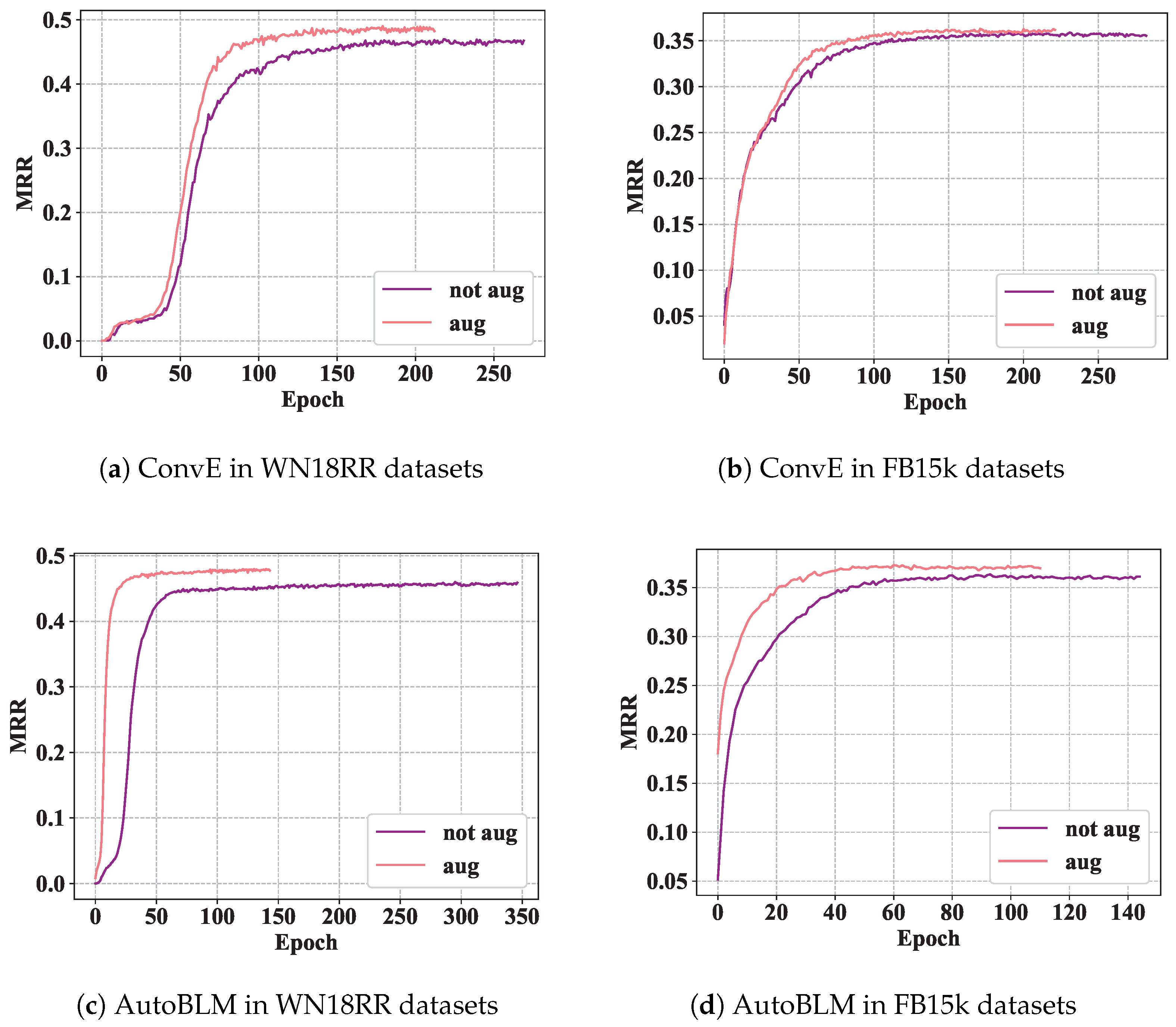
Figure 3 shows the validation MRR trajectories for ConvE [13] and AutoBLM [37] on both datasets. Because the archived early-stopping epochs cannot be audited against all four plotted ranges, we use these trajectories only as qualitative illustrations and do not report numerical epoch savings. These trajectories are not used as uncertainty estimates.

The controlled results show whether the fixed rule-derived training evidence benefits each decoder under matched optimization conditions. The observed effect is decoder- and dataset-dependent, so the evidence supports a conditional augmentation benefit rather than uniform superiority across KGE models or datasets.

4.3. Additional Comparison Analysis

Table 4. Additional comparison analysis under the settings used in the original KnowAug and KG-Mixup papers. † denotes a result taken from the cited original paper; unmarked rows are local runs from this study. KnowAug and KG-Mixup were not rerun. All values are rounded to three decimals.

Setting	Dataset	Method	MRR	Hits@1	Hits@10
KnowAug	WN18RR	ComplEx †	0.437	0.393	0.526
		Local Base	0.436	0.392	0.526
		KnowAug–ComplEx †	0.453	0.414	0.535
		Ours–ComplEx	0.456	0.424	0.543
	FB15k-237	ComplEx †	0.317	0.224	0.504
		Local Base	0.319	0.227	0.506
		KnowAug–ComplEx †	0.331	0.239	0.516
		Ours–ComplEx	0.340	0.252	0.522
KG-Mixup	FB15k-237	ConvE †	0.330	0.240	0.512
		Local Base	0.331	0.242	0.513
		KG-Mixup–ConvE †	0.343	0.250	0.531
		Ours–ConvE	0.351	0.258	0.537
Additional ConvE	WN18RR	Local Base	0.436	0.421	0.523
		Ours–ConvE	0.477	0.448	0.541

is a separate additional analysis and is not part of the main controlled experiment reported in Table 2 and Table 3. For this analysis, we run Local Base and Ours with ComplEx or ConvE using the dataset, scorer, validation-based model selection, and standard filtered evaluation used in the corresponding KnowAug and KG-Mixup papers. KnowAug and KG-Mixup themselves are not rerun. Values marked with † are taken from the cited original papers; all unmarked values are local results from this study.

For this additional analysis only, the filter set is ${\mathcal{T}}_{\mathrm{train}}\cup {\mathcal{T}}_{\mathrm{valid}}\cup {\mathcal{T}}_{\mathrm{test}}$, without adding ${\mathcal{T}}_A$. Validation or test triples that also occur in the generated augmentation set therefore remain in the evaluation, following the original evaluation settings. The fixed augmentation sets contain 987 triples for WN18RR and 14,389 triples for FB15k-237. Their overlaps with the validation and test sets are 248 and 224 triples, respectively, on WN18RR and 2783 and 2674 triples, respectively, on FB15k-237. The augmentation procedure itself still uses only the training graph and never checks held-out membership during candidate generation.

Within the local rows, Ours improves MRR over Local Base by 0.020 and 0.021 with ComplEx on WN18RR and FB15k-237, respectively. With ConvE, the corresponding local differences are 0.020 on FB15k-237 and 0.041 on WN18RR. The unaugmented local MRR differs from the corresponding original-paper value by 0.001 on WN18RR and by at most 0.002 on FB15k-237. Although the Ours rows have higher point estimates than the marked KnowAug and KG-Mixup rows, these descriptive differences do not isolate implementation and training effects because the external methods were not rerun. The KG-Mixup paper does not report WN18RR; the final two rows therefore provide only a Local Base/Ours comparison.

4.4. Parameter Sensitivity

We examine the rule-retention threshold $\mathcal{M}$ and the augmentation weight $\lambda$.

4.4.1. Rule Threshold

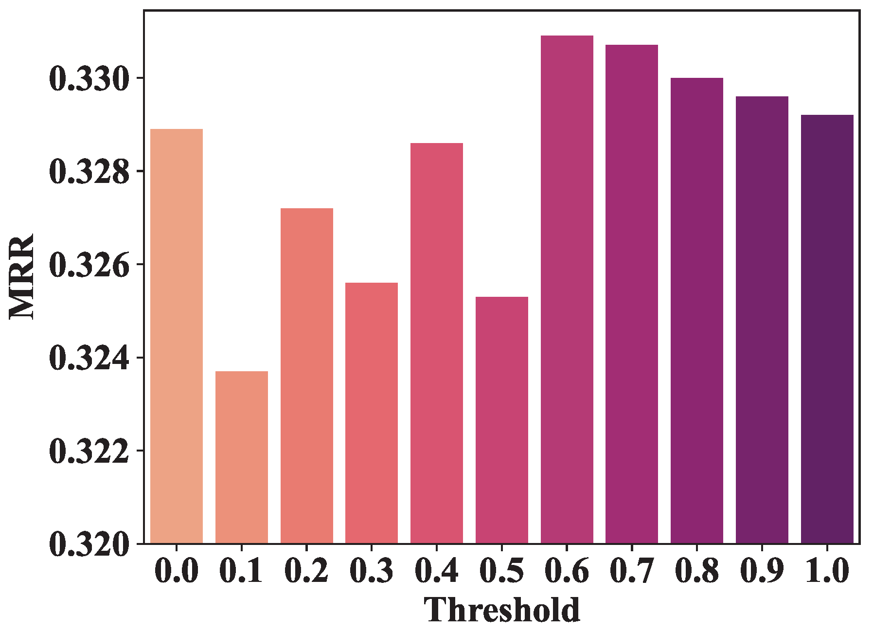
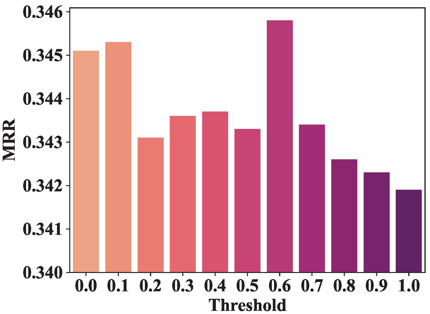
The threshold $\mathcal{M}$ controls which rules are retained. A high value favors reliable rules but may discard useful patterns, whereas a low value admits weaker rules. We test $\mathcal{M}\in \{0,0.1,\dots ,0.9\}$ with TransE [11] and ComplEx [12] on FB15k-237. Figure 4 and Figure 5 report validation MRR, the metric used for model selection.

The value $\mathcal{M}=1$ removes all rules and therefore uses only the original training data. Figure 4 reports the TransE results, and Figure 5 reports the ComplEx results. Both plots attain their best MRR at $\mathcal{M}=0.6$. When $\mathcal{M}<0.6$, less reliable rules can introduce noise, whereas $\mathcal{M}>0.6$ can discard useful rules.

4.4.2. Augmentation Weight

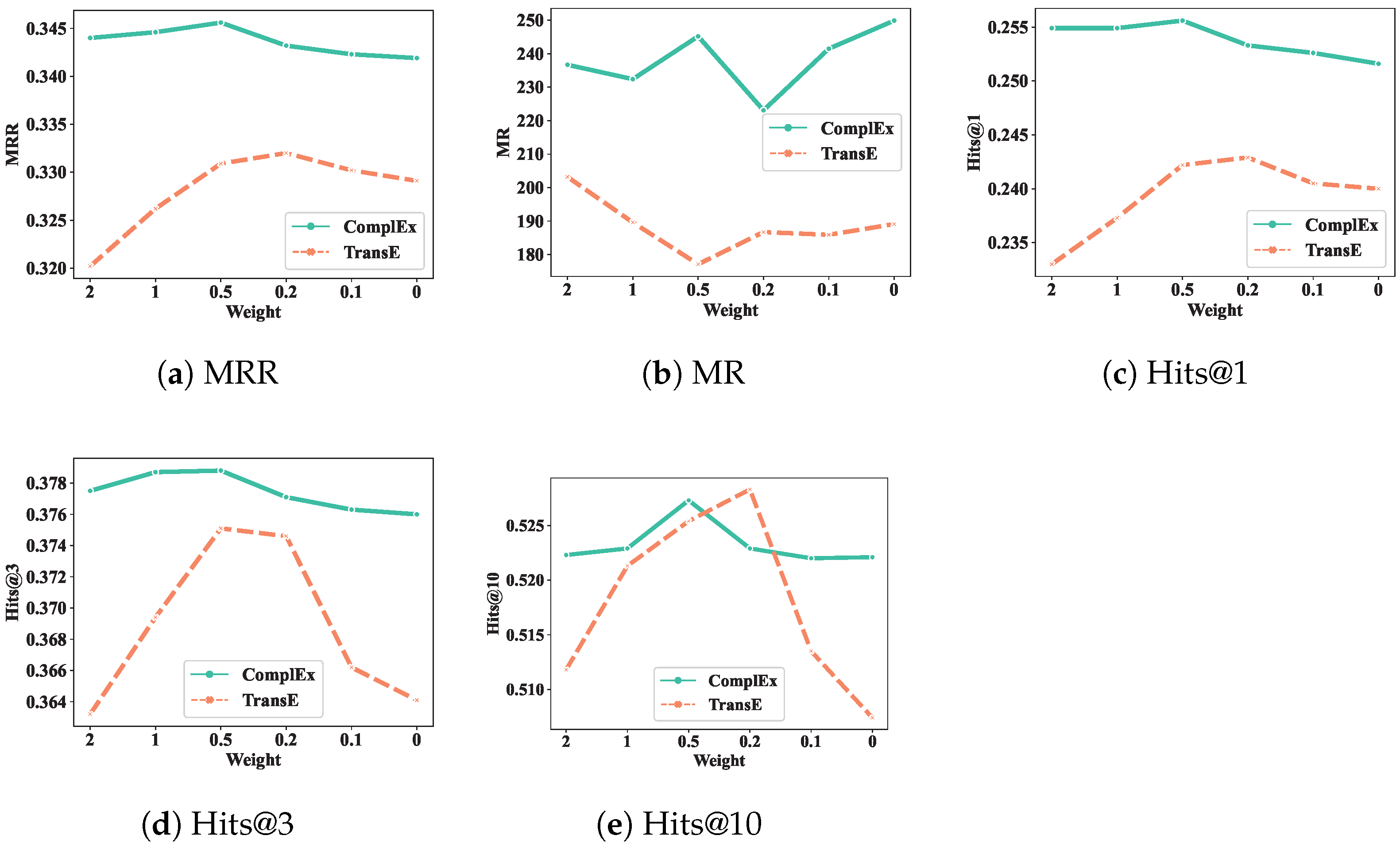
Augmented triples add multi-hop evidence but may also add noise. The weight $\lambda$ balances the original and augmented losses. We test $\lambda \in \{2,1,0.5,0.2,0.1\}$ on FB15k-237; Figure 6 reports the results.

Figure 6a reports MRR, Figure 6b reports MR, and Figure 6c–e report Hits@1, Hits@3, and Hits@10, respectively. Higher values are better for MRR and Hits@k, whereas lower values are better for MR. Across the five panels, assigning an excessively large weight to augmented data degrades several metrics, while $\lambda$ values of approximately $0.2$–$0.5$ provide the best overall balance.

4.5. Ablation

Table 5. Available AutoBLM ablation results on FB15k-237. Candidate ranking and reliability weighting are jointly enabled in the complete framework and are not isolated in this table.

Variant	MR	MRR	Hits@1	Hits@3	Hits@10
Base KGE	171	0.362	0.269	0.399	0.550
Random multi-hop augmentation	197	0.328	0.236	0.360	0.510
Rule-induced augmentation without candidate control	174	0.349	0.255	0.384	0.538
Complete framework	156	0.372	0.278	0.412	0.557

reports the available four-way AutoBLM ablation on FB15k-237. It distinguishes uncontrolled multi-hop augmentation, unranked rule-induced augmentation, and the complete candidate-control pipeline.

Under matched walk and retained-triple budgets, guided sampling improves MRR over uniform sampling by $0.003\pm 0.0001$ on WN18RR and $0.002\pm 0.0001$ on FB15k-237. Both comparisons use AutoBLM, retain 987 and 14,389 augmented triples, respectively, and report variation over KGE training seeds 41, 42, and 43 for augmentation sets generated with seed 42. The available experiments do not isolate the five reliability terms individually; we therefore describe them as parts of the implemented composite score rather than claiming a separately measured causal contribution for each term.

4.6. Efficiency

Table 6. Fixed-budget relative efficiency comparison. For each dataset, the recorded Base KGE training time is normalized to 1.00. Offline/Base is the recorded one-time augmentation cost divided by Base time; Training/Base and Total/Base are defined analogously. The timing archive does not preserve a physical unit, so only within-dataset ratios are reported. A double dash denotes this value is null.

Dataset	Variant	Offline/Base	Training/Base	Total/Base	$\mathbf{\Delta }$MRR
WN18RR	Base KGE	–	1.00	1.00	–
	Uniform augmentation	0.37	0.46	0.83	$+0.009$
	Ours	0.37	0.49	0.86	$+0.012$
FB15k-237	Base KGE	–	1.00	1.00	–
	Uniform augmentation	0.31	0.82	1.14	$+0.003$
	Ours	0.31	0.82	1.14	$+0.005$

compares Base KGE, uniform augmentation, and the complete method with AutoBLM and matched KGE settings at the fixed maximum walk budget $N=2000$. The two augmentation variants use the same walk and retained-triple budgets. AnyBURL is excluded from this runtime table because it was not executed in our environment and uses a different prediction interface; cross-publication runtime values would confound hardware and implementation differences.

On WN18RR, the shorter KGE training record offsets the one-time offline stage, yielding Total/Base ratios of 0.83 and 0.86 for uniform and guided augmentation, respectively. On FB15k-237, both augmentation variants have a Total/Base ratio of 1.14; the guided method provides the larger MRR gain ($+0.005$ versus $+0.003$). These fixed-budget ratios distinguish the reusable one-time augmentation cost from KGE training cost, but they do not establish a multi-budget scaling curve or scalability to substantially larger or dynamic knowledge graphs.

5. Discussion

The controlled Base/Aug comparisons test a fixed set of weighted rule-derived triples across decoders under matched optimization conditions. Together with the sensitivity and ablation results, they show that candidate quality and training weight affect whether augmentation helps. Unfiltered or overweighted triples can reduce performance, and the observed gains vary across decoders and datasets. The evidence therefore supports a conditional benefit rather than uniform superiority.

The separate additional analysis in Table 4 provides descriptive context against KnowAug and KG-Mixup and is not part of the main controlled experiment. The close agreement between each Local Base result and the corresponding unaugmented result from the original paper supports the consistency of the scorer and evaluation setup. Ours produces higher point estimates than the augmented results in the original papers for the reported comparisons. However, the external augmentation methods were not rerun, so the remaining differences may reflect implementation and training details in addition to the augmentation method. These additional results should therefore not be interpreted as a comparison of all the methods within one codebase or as the primary evidence for the method.

Rule induction and candidate generation run once offline, and the resulting weighted triples can be reused across scoring models and training runs. This separation amortizes the offline cost over repeated KGE training without replacing the deployed embedding predictor with a separate rule reasoner. The fixed-budget efficiency ratios nevertheless apply only to WN18RR and FB15k-237; substantially larger or frequently changing KGs may require lower walk budgets, incremental rule updates, or more scalable candidate indexing.

The study has six limitations. First, the static benchmarks do not establish scalability to industrial or rapidly changing KGs. Second, the timing archive lacks absolute units and memory profiles, so only within-dataset ratios can be compared. Third, each augmentation variant uses one sampling seed; the reported deviations capture KGE training variability but not rule-sampling uncertainty. Fourth, KnowAug and KG-Mixup were not rerun, so comparisons with their original-paper results are not controlled within one codebase. Fifth, the additional analysis retains the 248 validation and 224 test overlaps on WN18RR and the 2,783 validation and 2,674 test overlaps on FB15k-237 to follow the original evaluation settings. These results should not be interpreted as a leakage-free test of unseen facts. Sixth, the experiments do not isolate the five reliability terms individually or test their transfer across different relation distributions. Future work should evaluate larger dynamic KGs, multiple augmentation seeds, external methods in one shared codebase, and adaptive weighting without exposing held-out test facts.

6. Conclusions

We presented a rule-guided augmentation method for knowledge graph completion. Target-relation-guided random walks provide Horn rules, which generate candidate training triples. A candidate-level score combines smoothed rule reliability, normalized support, type validity, path consistency, and redundancy. This score controls each retained triple’s training weight, while the embedding model remains the final link predictor. Controlled Base/Aug comparisons on WN18RR and FB15k-237 evaluate five scoring functions under identical training pipelines and report mean and standard deviation over three KGE training seeds. Under this protocol, the augmentation increases MRR by 0.001–0.012 on WN18RR and by 0.001–0.005 on FB15k-237. A separate additional analysis provides descriptive context against the original-paper KnowAug and KG-Mixup results; because these external methods were not rerun, this analysis is not treated as a controlled main result. The sensitivity analysis indicates that the benefit depends on the reliability and weight of the generated triples: a low rule threshold may introduce noise, while an excessively high threshold may remove useful rules. The AutoBLM comparison shows the difference between guided and uniform sampling under matched augmentation budgets. The four-way ablation evaluates candidate control as a whole and does not isolate the five reliability terms. The efficiency analysis separates reusable offline augmentation from KGE training through within-dataset fixed-budget ratios.

References

1. Zhu, G.; Iglesias, C.A. Exploiting semantic similarity for named entity disambiguation in knowledge graphs. Expert Syst. Appl. 2018, 101, 8–24. [Google Scholar] [CrossRef] [Scilit]
2. Hu, S.; Zou, L.; Yu, J.X.; Wang, H.; Zhao, D. Answering natural language questions by subgraph matching over knowledge graphs. IEEE Trans. Knowl. Data Eng. 2017, 30, 824–837. [Google Scholar] [CrossRef] [Scilit]
3. Wang, H.; Zhang, F.; Wang, J.; Zhao, M.; Li, W.; Xie, X.; Guo, M. Exploring high-order user preference on the knowledge graph for recommender systems. ACM Trans. Inf. Syst. (TOIS) 2019, 37, 1–26. [Google Scholar] [CrossRef] [Scilit]
4. Rosa, R.L.; Schwartz, G.M.; Ruggiero, W.V.; Rodríguez, D.Z. A knowledge-based recommendation system that includes sentiment analysis and deep learning. IEEE Trans. Ind. Inform. 2018, 15, 2124–2135. [Google Scholar] [CrossRef] [Scilit]
5. Marino, K.; Salakhutdinov, R.; Gupta, A. The more you know: Using knowledge graphs for image classification. arXiv 2016, arXiv:1612.04844. [Google Scholar]
6. Bollacker, K.; Evans, C.; Paritosh, P.; Sturge, T.; Taylor, J. Freebase: A collaboratively created graph database for structuring human knowledge. In Proceedings of the 2008 ACM SIGMOD International Conference on Management of Data; Association for Computing Machinery: New York, NY, USA, 2008; pp. 1247–1250. [Google Scholar]
7. Miller, G.A. WordNet: An Electronic Lexical Database; MIT Press: Cambridge, MA, USA, 1998. [Google Scholar]
8. Vrandečić, D.; Krötzsch, M. Wikidata: A free collaborative knowledgebase. Commun. ACM 2014, 57, 78–85. [Google Scholar]
9. Mahdisoltani, F.; Biega, J.; Suchanek, F. Yago3: A knowledge base from multilingual wikipedias. In Proceedings of the 7th Biennial Conference on Innovative Data Systems Research, CIDR Conference, Asilomar, CA, USA, 4–7 January 2014. [Google Scholar]
10. Wang, Q.; Mao, Z.; Wang, B.; Guo, L. Knowledge graph embedding: A survey of approaches and applications. IEEE Trans. Knowl. Data Eng. 2017, 29, 2724–2743. [Google Scholar] [CrossRef] [Scilit]
11. Bordes, A.; Usunier, N.; Garcia-Duran, A.; Weston, J.; Yakhnenko, O. Translating embeddings for modeling multi-relational data. Adv. Neural Inf. Process. Syst. 2013, 26, 2787–2795. [Google Scholar]
12. Trouillon, T.; Welbl, J.; Riedel, S.; Gaussier, É.; Bouchard, G. Complex embeddings for simple link prediction. In Proceedings of the International Conference on Machine Learning; PMLR: Cambridge, MA, USA, 2016; pp. 2071–2080. [Google Scholar]
13. Dettmers, T.; Minervini, P.; Stenetorp, P.; Riedel, S. Convolutional 2d knowledge graph embeddings. In Proceedings of the AAAI Conference on Artificial Intelligence; AAAI Press: Palo Alto, CA, USA, 2018; Volume 32. [Google Scholar]
14. Schlichtkrull, M.; Kipf, T.N.; Bloem, P.; Berg, R.v.d.; Titov, I.; Welling, M. Modeling relational data with graph convolutional networks. In Proceedings of the European Semantic Web Conference; Springer: Berlin/Heidelberg, Germany, 2018; pp. 593–607. [Google Scholar]
15. Li, Z.; Liu, H.; Zhang, Z.; Liu, T.; Xiong, N.N. Learning Knowledge Graph Embedding with Heterogeneous Relation Attention Networks. IEEE Trans. Neural Netw. Learn. Syst. 2022, 33, 3961–3973. [Google Scholar] [CrossRef] [Scilit] [PubMed]
16. Wu, J.; Shi, W.; Cao, X.; Chen, J.; Lei, W.; Zhang, F.; Wu, W.; He, X. DisenKGAT: Knowledge graph embedding with disentangled graph attention network. In Proceedings of the 30th ACM International Conference on Information & Knowledge Management; Association for Computing Machinery: New York, NY, USA, 2021; pp. 2140–2149. [Google Scholar]
17. Yang, Z.; Ding, M.; Zhou, C.; Yang, H.; Zhou, J.; Tang, J. Understanding negative sampling in graph representation learning. In Proceedings of the 26th ACM SIGKDD International Conference on Knowledge Discovery & Data Mining; Association for Computing Machinery: New York, NY, USA, 2020; pp. 1666–1676. [Google Scholar]
18. Meilicke, C.; Chekol, M.W.; Ruffinelli, D.; Stuckenschmidt, H. Anytime Bottom-Up Rule Learning for Knowledge Graph Completion. In Proceedings of the Twenty-Eighth International Joint Conference on Artificial Intelligence; AAAI Press: Palo Alto, CA, USA, 2019; pp. 3137–3143. [Google Scholar] [CrossRef] [Scilit] [PubMed]
19. Yang, F.; Yang, Z.; Cohen, W.W. Differentiable Learning of Logical Rules for Knowledge Base Reasoning. In Proceedings of the Advances in Neural Information Processing Systems; Neural Information Processing Systems Foundation, Inc.: San Diego, CA, USA, 2017; Volume 30. [Google Scholar]
20. Li, G.; Sun, Z.; Qian, L.; Guo, Q.; Hu, W. Rule-Based Data Augmentation for Knowledge Graph Embedding. AI Open 2021, 2, 186–196. [Google Scholar] [CrossRef] [Scilit]
21. Shomer, H.; Jin, W.; Wang, W.; Tang, J. Toward Degree Bias in Embedding-Based Knowledge Graph Completion. In Proceedings of the ACM Web Conference 2023; Association for Computing Machinery: New York, NY, USA, 2023; pp. 705–715. [Google Scholar] [CrossRef] [Scilit]
22. Yang, B.; Yih, W.t.; He, X.; Gao, J.; Deng, L. Embedding entities and relations for learning and inference in knowledge bases. arXiv 2014, arXiv:1412.6575. [Google Scholar]
23. Vashishth, S.; Sanyal, S.; Nitin, V.; Talukdar, P. Composition-based multi-relational graph convolutional networks. arXiv 2019, arXiv:1911.03082. [Google Scholar]
24. Zhang, Z.; Wang, J.; Ye, J.; Wu, F. Rethinking graph convolutional networks in knowledge graph completion. In Proceedings of the ACM Web Conference 2022; Association for Computing Machinery: New York, NY, USA, 2022; pp. 798–807. [Google Scholar]
25. Mikolov, T.; Chen, K.; Corrado, G.; Dean, J. Efficient estimation of word representations in vector space. arXiv 2013, arXiv:1301.3781. [Google Scholar]
26. Tang, J.; Qu, M.; Wang, M.; Zhang, M.; Yan, J.; Mei, Q. Line: Large-scale information network embedding. In Proceedings of the 24th International Conference on World Wide Web; International World Wide Web Conferences Steering Committee: Geneva, Switzerland, 2015; pp. 1067–1077. [Google Scholar]
27. Perozzi, B.; Al-Rfou, R.; Skiena, S. Deepwalk: Online learning of social representations. In Proceedings of the 20th ACM SIGKDD International Conference on Knowledge Discovery and Data Mining; Association for Computing Machinery: New York, NY, USA, 2014; pp. 701–710. [Google Scholar]
28. Grover, A.; Leskovec, J. node2vec: Scalable feature learning for networks. In Proceedings of the 22nd ACM SIGKDD International Conference on Knowledge Discovery and Data Mining; Association for Computing Machinery: New York, NY, USA, 2016; pp. 855–864. [Google Scholar]
29. Gilmer, J.; Schoenholz, S.S.; Riley, P.F.; Vinyals, O.; Dahl, G.E. Neural message passing for quantum chemistry. In Proceedings of the International Conference on Machine Learning; PMLR: Cambridge, MA, USA, 2017; pp. 1263–1272. [Google Scholar]
30. Veličković, P.; Fedus, W.; Hamilton, W.L.; Liò, P.; Bengio, Y.; Hjelm, R.D. Deep graph infomax. arXiv 2018, arXiv:1809.10341. [Google Scholar]
31. Cai, C.; Wang, D.; Wang, Y. Graph coarsening with neural networks. arXiv 2021, arXiv:2102.01350. [Google Scholar]
32. Jin, W.; Zhao, L.; Zhang, S.; Liu, Y.; Tang, J.; Shah, N. Graph condensation for graph neural networks. arXiv 2021, arXiv:2110.07580. [Google Scholar]
33. Liu, X.; Sun, D.; Wei, W. Alleviating the over-smoothing of graph neural computing by a data augmentation strategy with entropy preservation. Pattern Recognit. 2022, 132, 108951. [Google Scholar] [CrossRef] [Scilit]
34. Wu, H.; Wang, Z.; Wang, K.; Omran, P.G.; Li, J. Rule Learning over Knowledge Graphs: A Review. Trans. Graph Data Knowl. 2023, 1, 7:1–7:23. [Google Scholar] [CrossRef]
35. Liu, H.; Wang, Z.; Wang, K.; Zhang, X.; Feng, Z. Transfer Rule Learning over Large Knowledge Graphs. In Proceedings of the ACM on Web Conference 2025, New York, NY, USA, 28 April–2 May 2025; WWW ’25; Association for Computing Machinery: New York, NY, USA, 2025; pp. 2135–2143. [Google Scholar] [CrossRef] [Scilit]
36. Wang, Z.; Zhang, J.; Feng, J.; Chen, Z. Knowledge graph embedding by translating on hyperplanes. In Proceedings of the AAAI Conference on Artificial Intelligence; AAAI Press: Palo Alto, CA, USA, 2014; Volume 28. [Google Scholar]
37. Zhang, Y.; Yao, Q.; Kwok, J.T. Bilinear scoring function search for knowledge graph learning. IEEE Trans. Pattern Anal. Mach. Intell. 2022, 45, 1458–1473. [Google Scholar] [CrossRef] [Scilit] [PubMed]
38. Meilicke, C.; Fink, M.; Wang, Y.; Ruffinelli, D.; Gemulla, R.; Stuckenschmidt, H. Fine-Grained Evaluation of Rule- and Embedding-Based Systems for Knowledge Graph Completion. In Proceedings of the International Semantic Web Conference; Springer International Publishing: Berlin/Heidelberg, Germany, 2018; pp. 3–20. [Google Scholar]
39. Omran, P.G.; Wang, K.; Wang, Z. Scalable Rule Learning via Learning Representation. In Proceedings of the Twenty-Seventh International Joint Conference on Artificial Intelligence; AAAI Press: Palo Alto, CA, USA, 2018; pp. 2149–2155. [Google Scholar] [CrossRef] [Scilit] [PubMed]
Figure 1. A knowledge graph subgraph illustrating a daughter-in-law relation inferred from a two-hop relational path. Circles denote entities, and directed labeled edges denote relations.
Mathematics 14 02984 g001
Figure 2. Rule-based augmentation. (a) The training graph, with entities as circles and relations as labeled directed edges. (b) An observed head path and two sampled body paths used for rule induction. (c) Three induced relation rules; dashed circles denote entity variables. (d) Rule inference on a grounded body path; dashed edges denote candidate relations.
Mathematics 14 02984 g002
Figure 3. Validation MRR trajectories for Base and Aug variants using ConvE [13] and AutoBLM [37] on WN18RR and FB15k-237.
Mathematics 14 02984 g003
Figure 4. Validation MRR under different rule-retention thresholds M for TransE on FB15k-237.
Mathematics 14 02984 g004
Figure 5. Validation MRR under different rule-retention thresholds M for ComplEx on FB15k-237.
Mathematics 14 02984 g005
Figure 6. Sensitivity to the augmentation weight λ for ComplEx on FB15k-237: (a) MRR, (b) MR, (c) Hits@1, (d) Hits@3, and (e) Hits@10.
Mathematics 14 02984 g006