Figure 1.
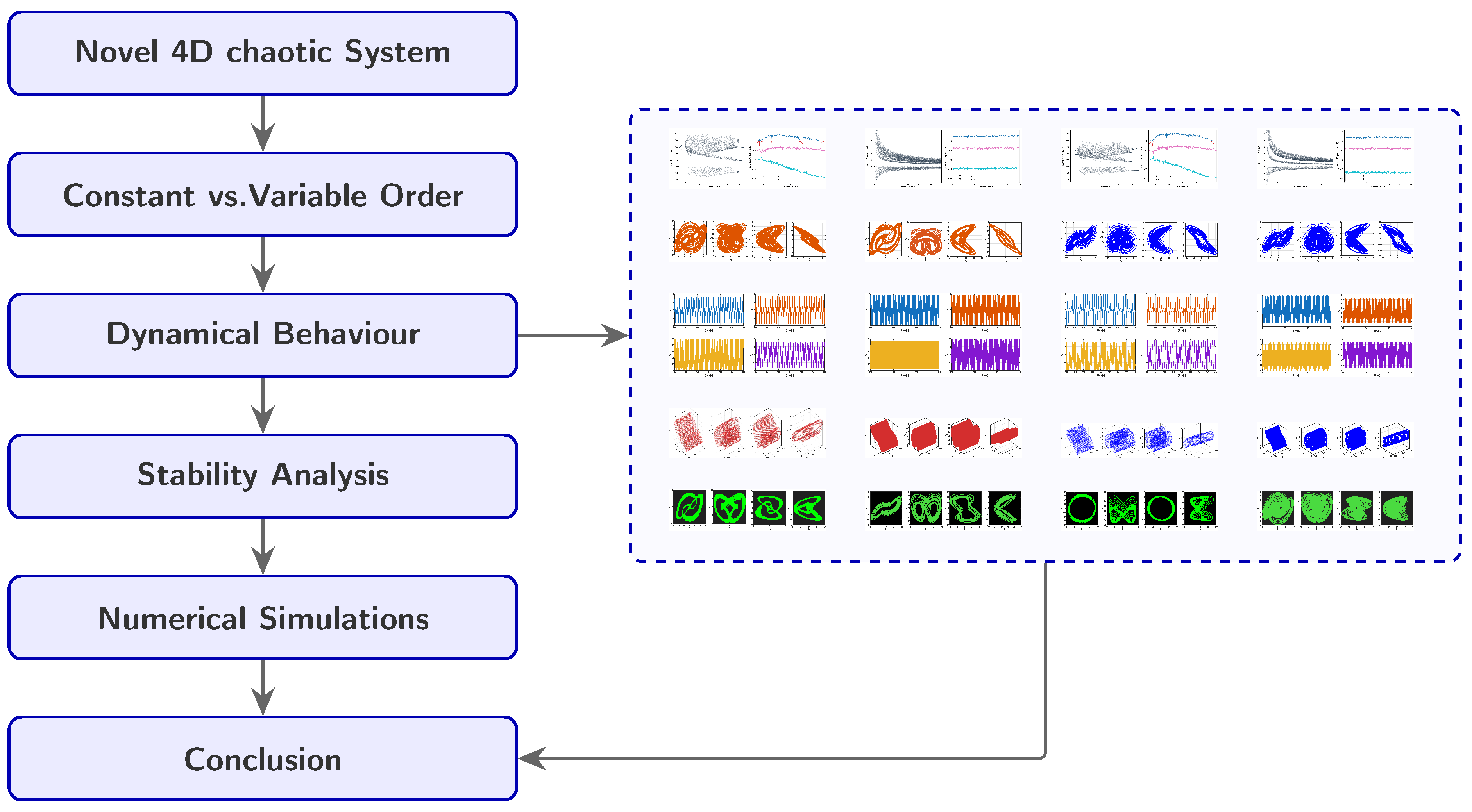
Methodology and dynamical analysis flowchart for the novel 4D chaotic system.
Figure 1.
Methodology and dynamical analysis flowchart for the novel 4D chaotic system.
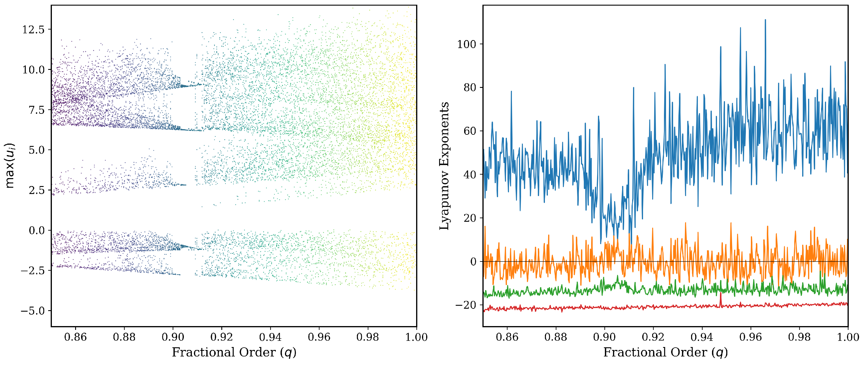
Figure 2.
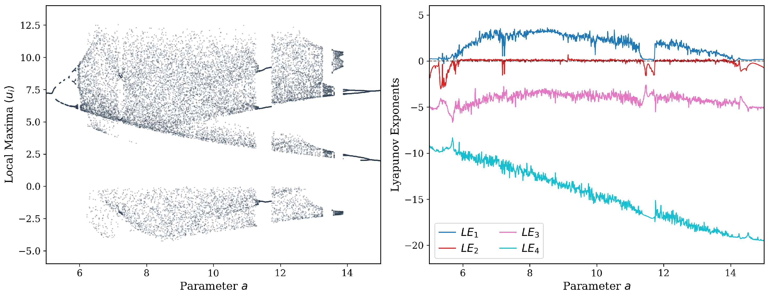
Variable. Bifurcation diagram (left) and corresponding Lyapunov exponents spectrum (right) as a function of the fractional order Case 1 evaluated at parameter a.
Figure 2.
Variable. Bifurcation diagram (left) and corresponding Lyapunov exponents spectrum (right) as a function of the fractional order Case 1 evaluated at parameter a.
Figure 3.
Variable. Bifurcation diagram (left) and corresponding Lyapunov exponents spectrum (right) as a function of the fractional order Case 1 evaluated at parameter c.
Figure 3.
Variable. Bifurcation diagram (left) and corresponding Lyapunov exponents spectrum (right) as a function of the fractional order Case 1 evaluated at parameter c.
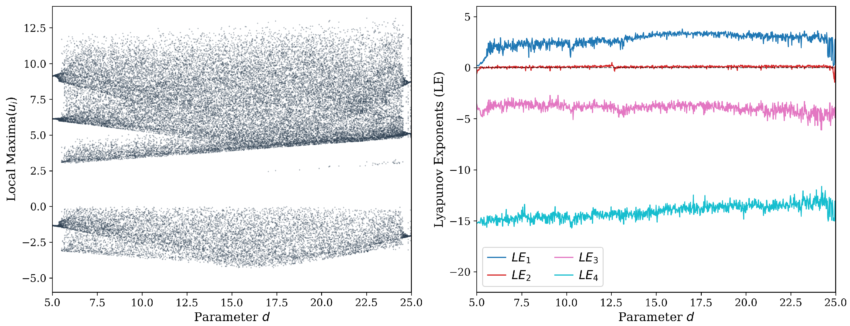
Figure 4.
Variable. Bifurcation diagram (left) and corresponding Lyapunov exponents spectrum (right) as a function of the fractional order Case 1 evaluated at parameter d.
Figure 4.
Variable. Bifurcation diagram (left) and corresponding Lyapunov exponents spectrum (right) as a function of the fractional order Case 1 evaluated at parameter d.
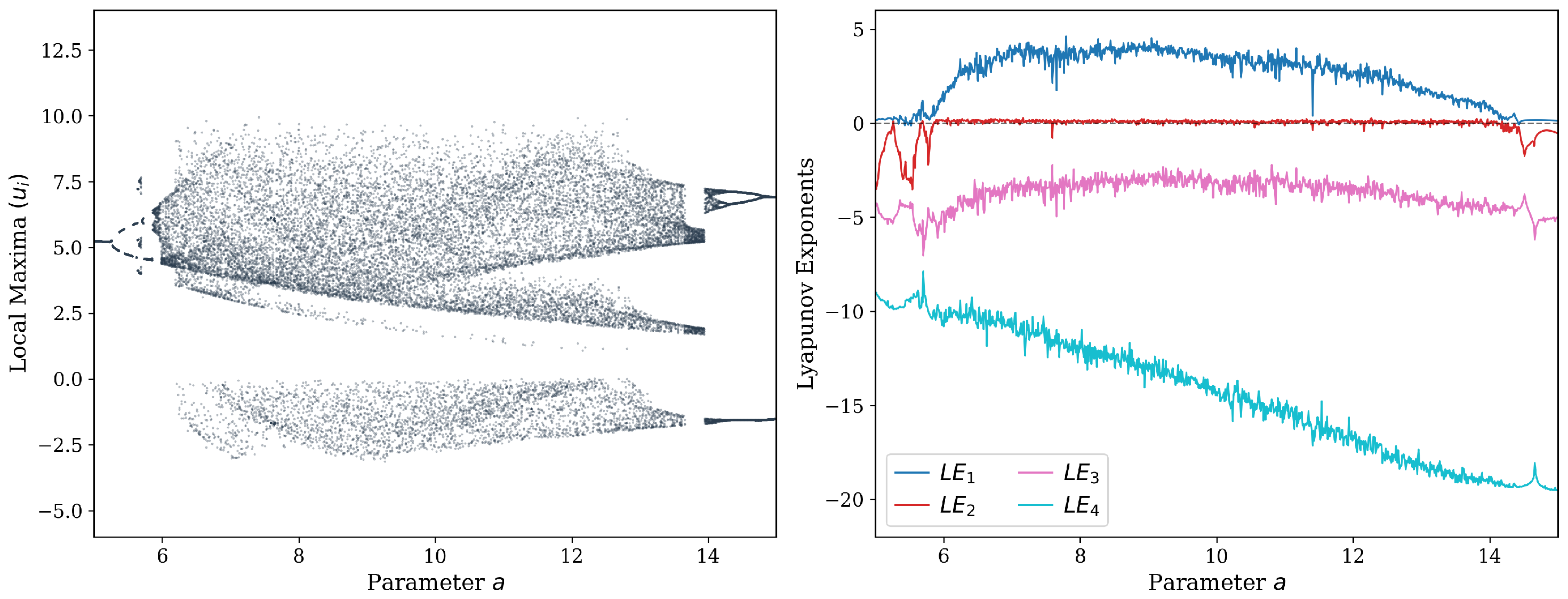
Figure 5.
Variable. Bifurcation diagram (left) and corresponding Lyapunov exponents spectrum (right) as a function of the fractional order Case 2 evaluated at parameter a.
Figure 5.
Variable. Bifurcation diagram (left) and corresponding Lyapunov exponents spectrum (right) as a function of the fractional order Case 2 evaluated at parameter a.
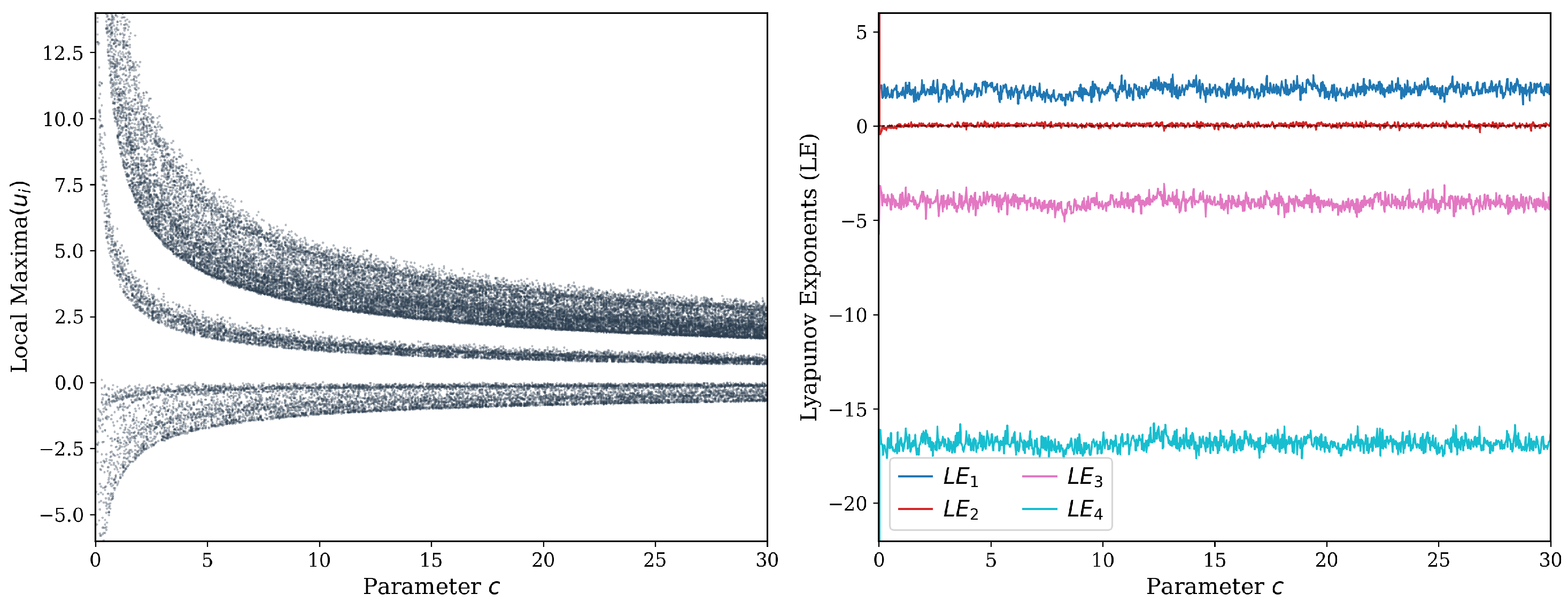
Figure 6.
Variable. Bifurcation diagram (left) and corresponding Lyapunov exponents spectrum (right) as a function of the fractional order Case 2 evaluated at parameter c.
Figure 6.
Variable. Bifurcation diagram (left) and corresponding Lyapunov exponents spectrum (right) as a function of the fractional order Case 2 evaluated at parameter c.
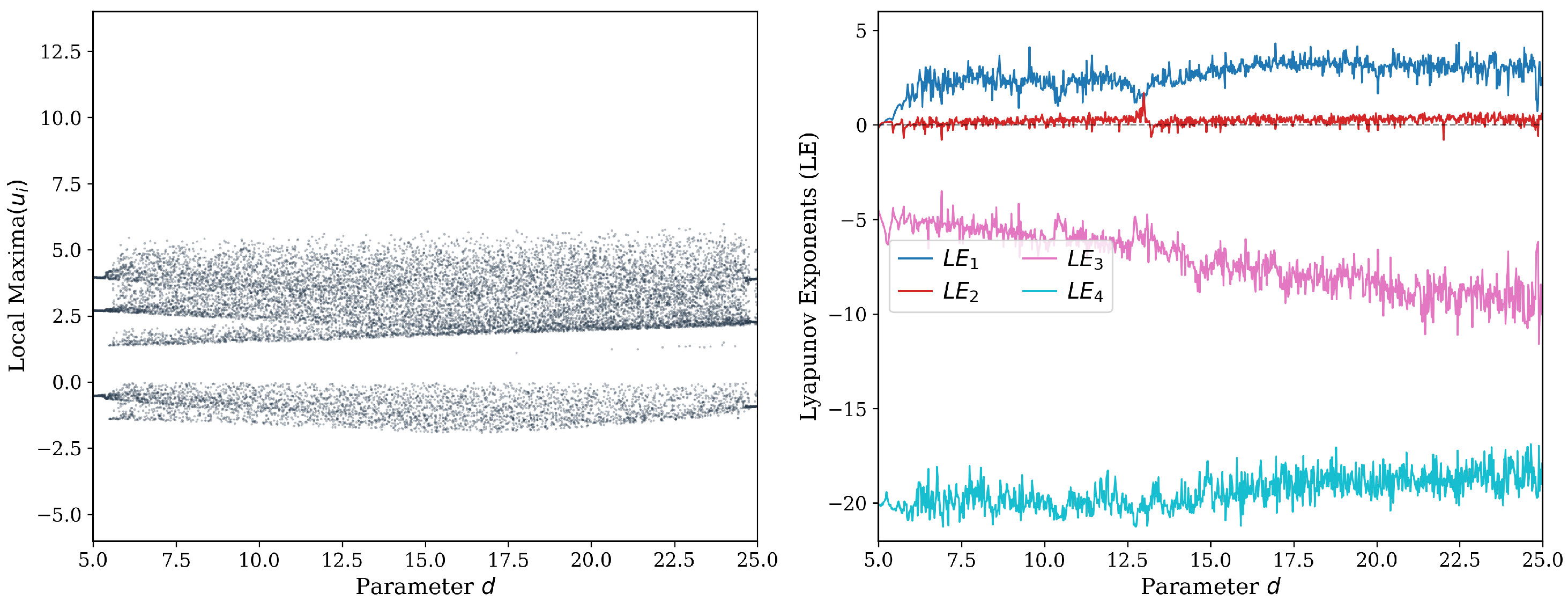
Figure 7.
Variable. Bifurcation diagram (left) and corresponding Lyapunov exponents spectrum (right) as a function of the fractional order Case 2 evaluated at parameter d.
Figure 7.
Variable. Bifurcation diagram (left) and corresponding Lyapunov exponents spectrum (right) as a function of the fractional order Case 2 evaluated at parameter d.
Figure 8.
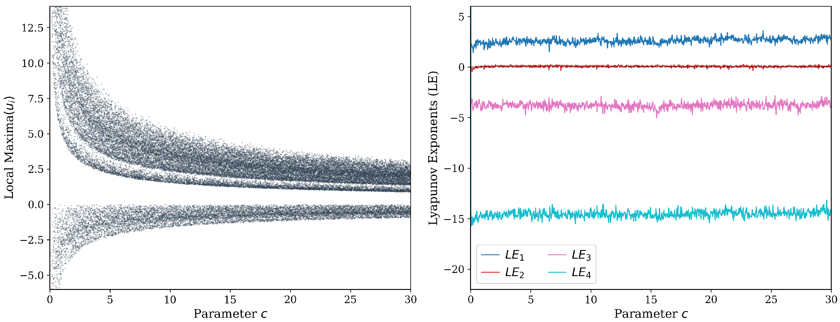
Constant. Bifurcation diagram (left) and corresponding Lyapunov exponents spectrum (right) as a function of the fractional order q.
Figure 8.
Constant. Bifurcation diagram (left) and corresponding Lyapunov exponents spectrum (right) as a function of the fractional order q.
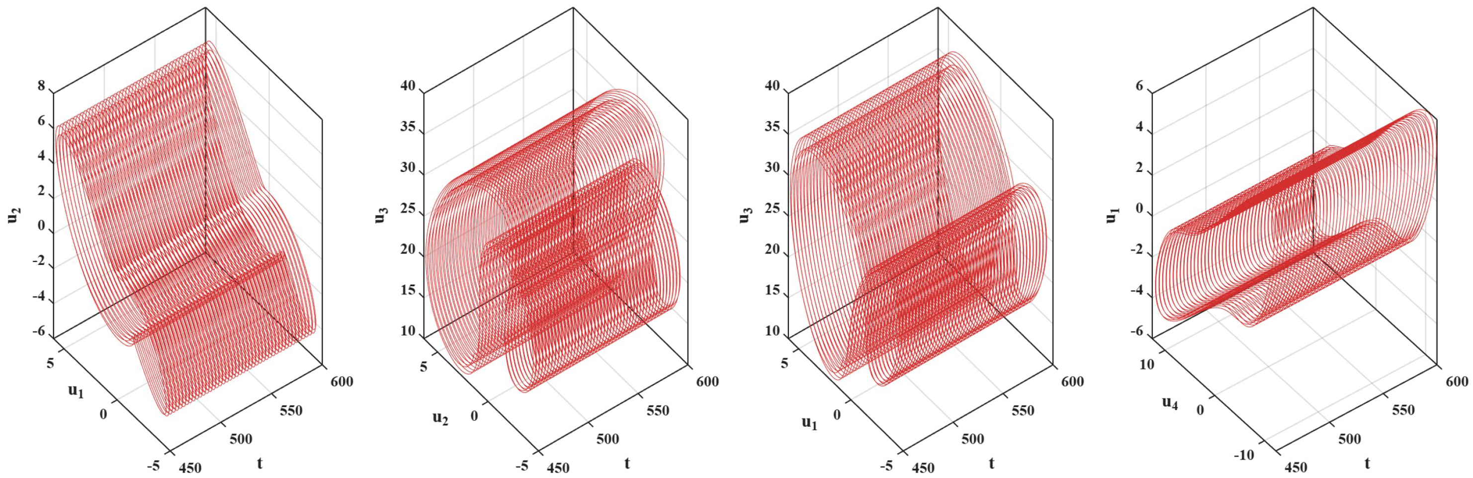
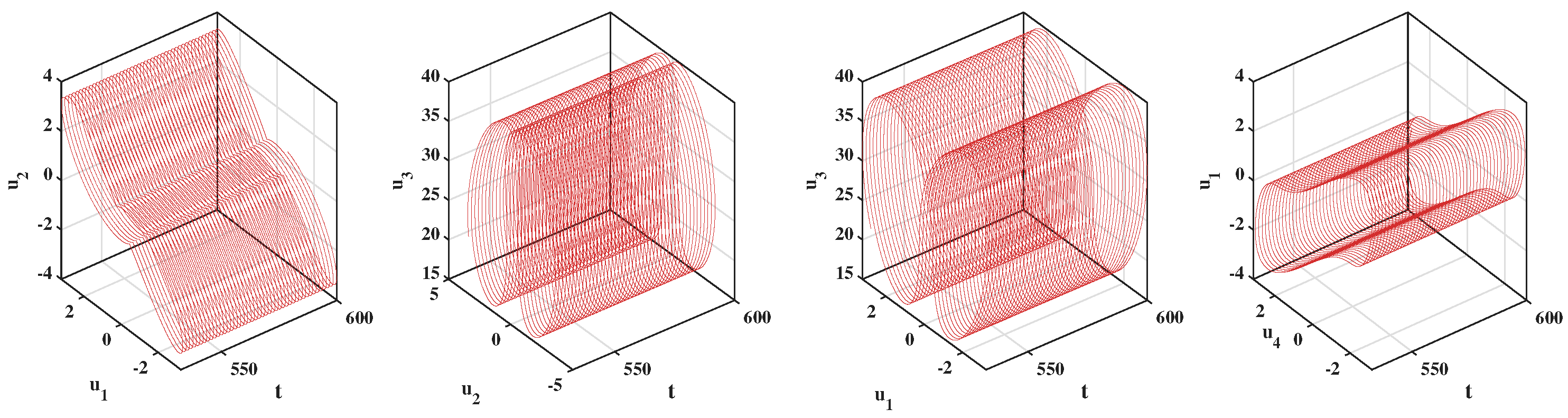
Figure 9.
3D dynamic trajectories of the system state components under Case 1.
Figure 9.
3D dynamic trajectories of the system state components under Case 1.
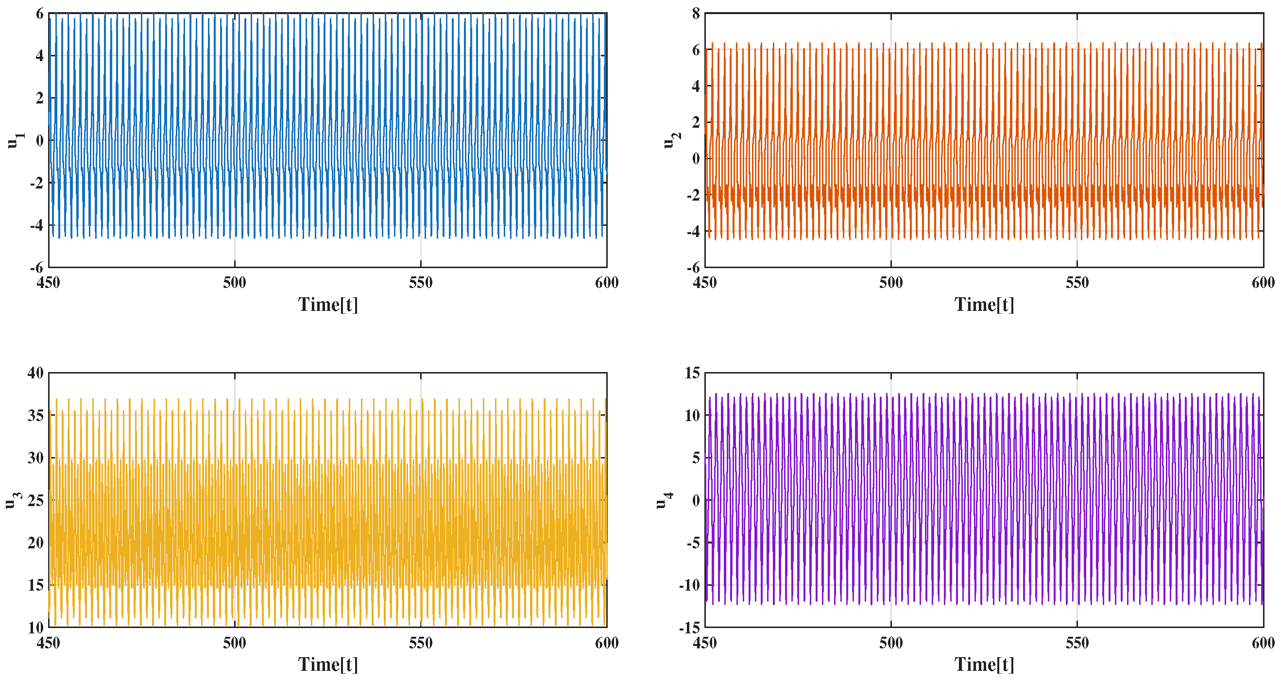
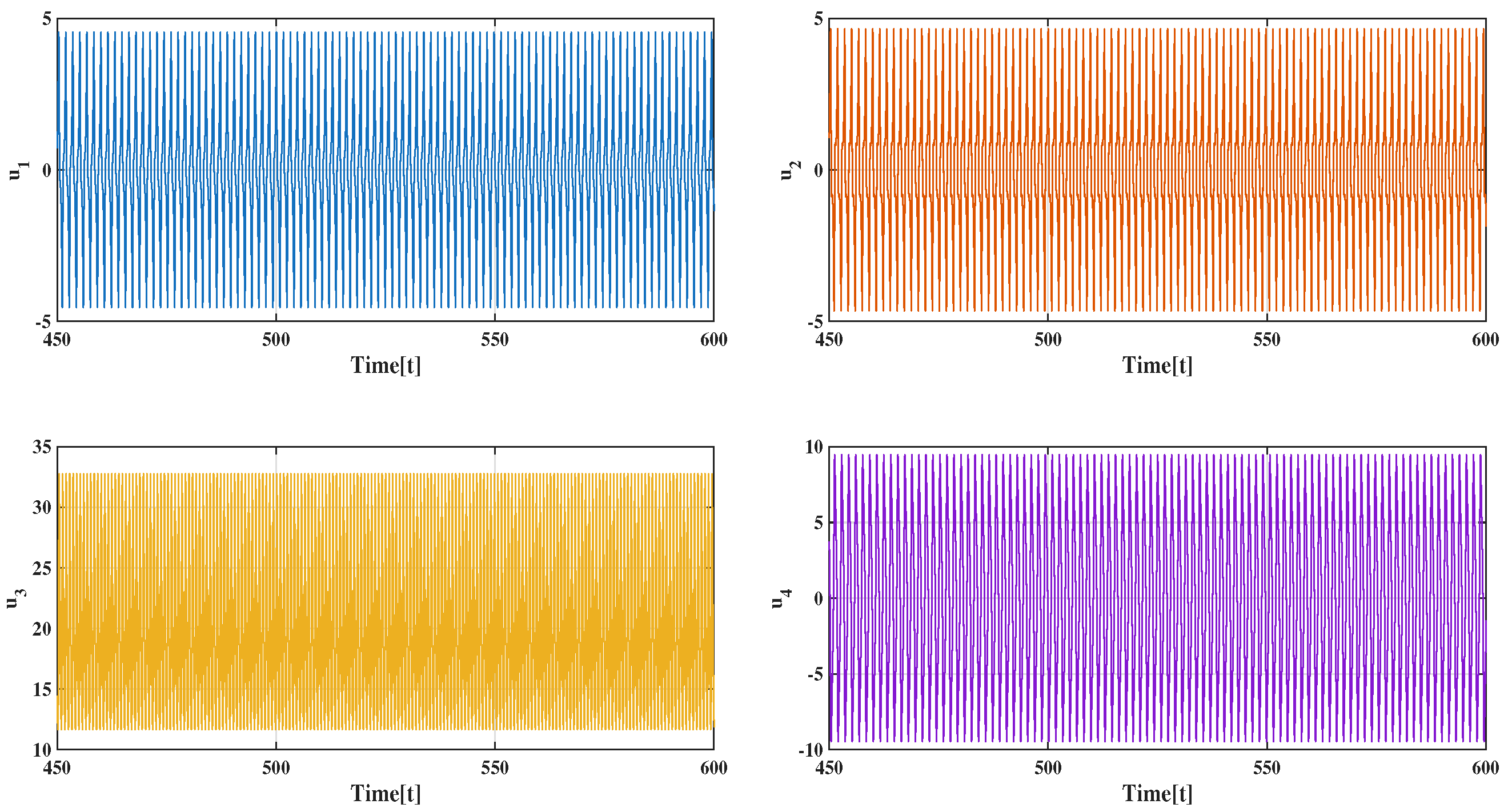
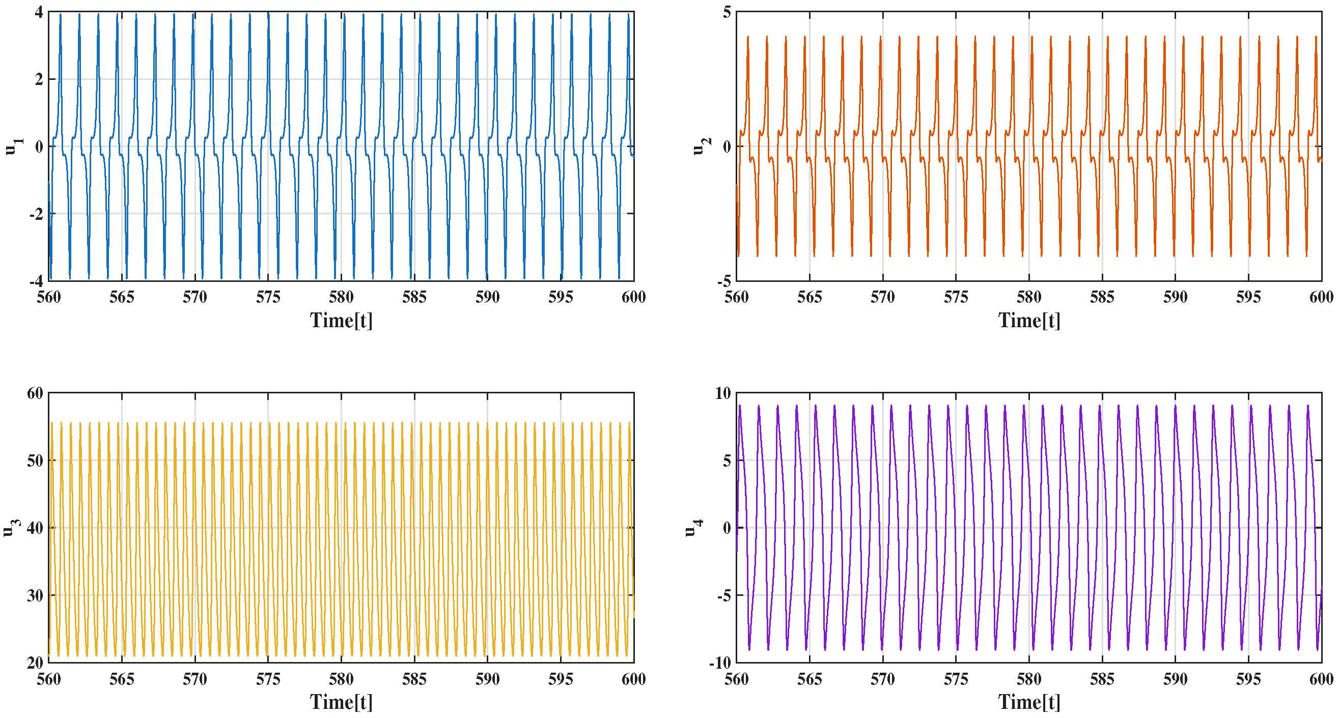
Figure 10.
Time-series evolution of the system for Case 1.
Figure 10.
Time-series evolution of the system for Case 1.
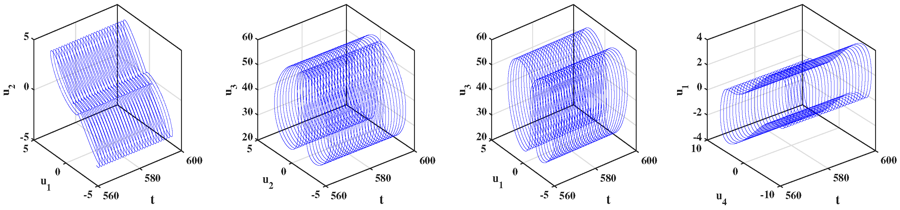
Figure 11.
3D dynamic trajectories of the system state components under .
Figure 11.
3D dynamic trajectories of the system state components under .
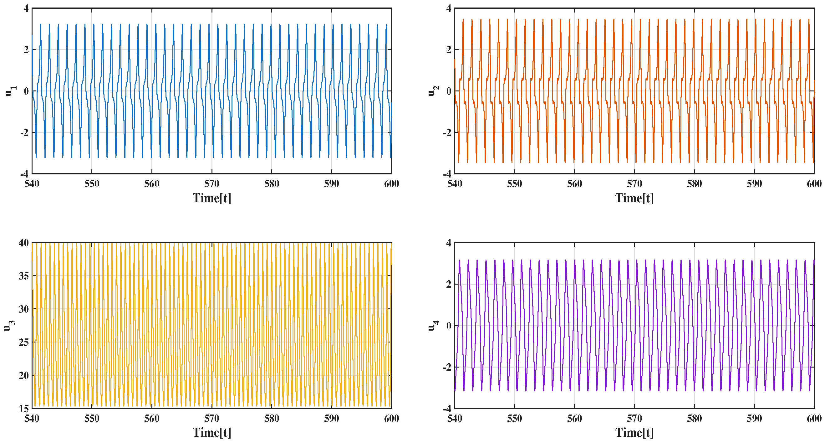
Figure 12.
Time-series evolution of the system for .
Figure 12.
Time-series evolution of the system for .
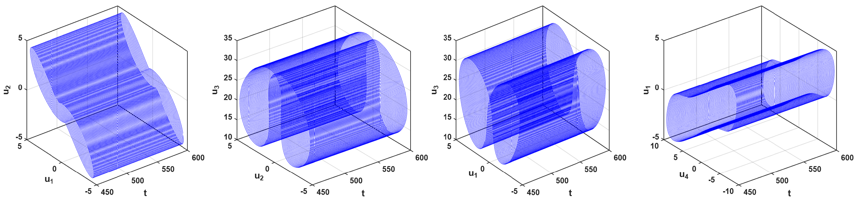
Figure 13.
3D phase-time portraits of the system state variables for Case 2.
Figure 13.
3D phase-time portraits of the system state variables for Case 2.
Figure 14.
Time-series evolution of the system for Case 2.
Figure 14.
Time-series evolution of the system for Case 2.
Figure 15.
3D phase-time portraits of the system state variables for .
Figure 15.
3D phase-time portraits of the system state variables for .
Figure 16.
Time-series evolution of the system for .
Figure 16.
Time-series evolution of the system for .
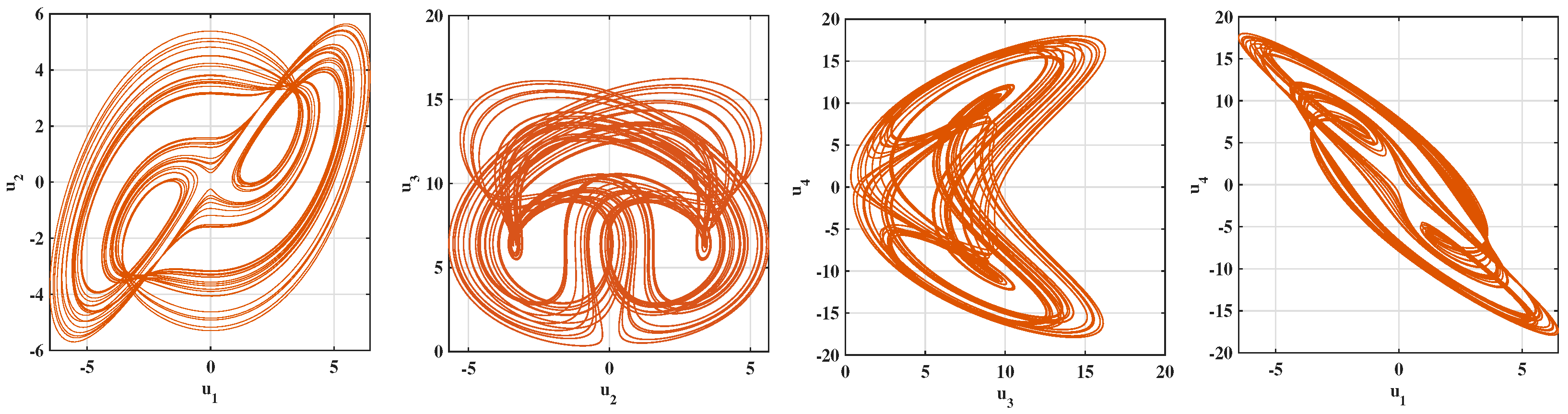
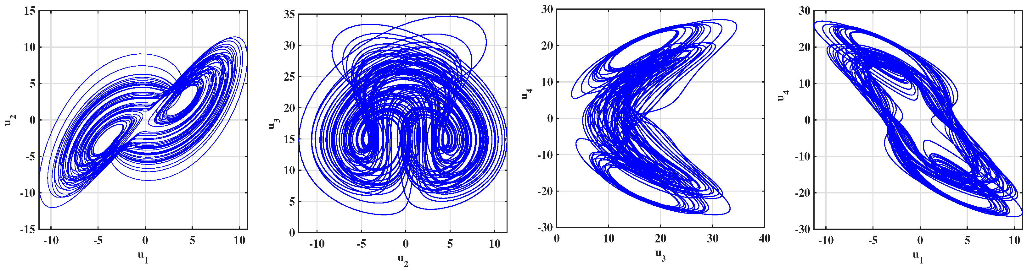
Figure 17.
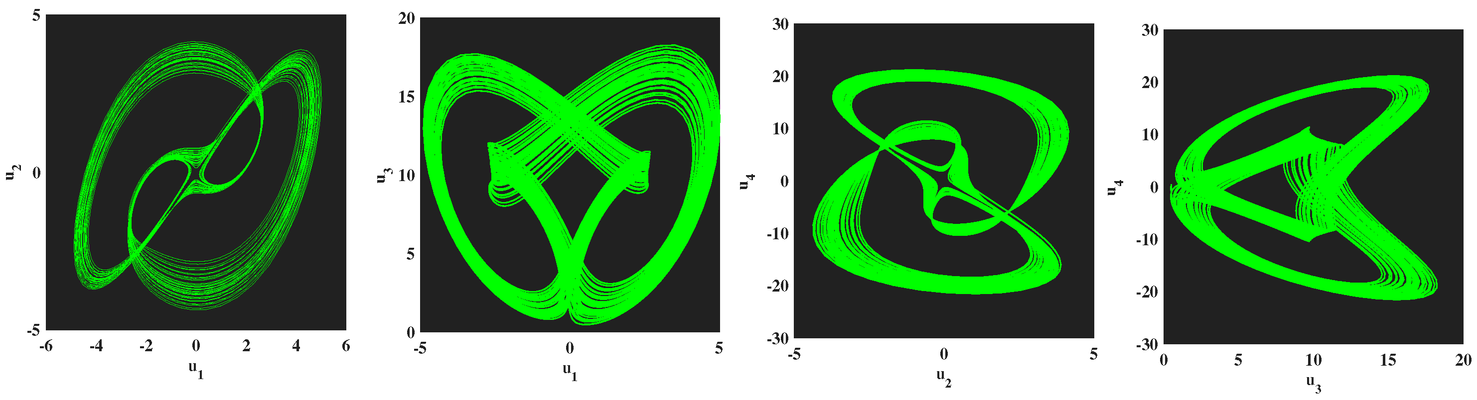
Phase portraits of the chaotic system’s attractor in various 2D projections for Case 1.
Figure 17.
Phase portraits of the chaotic system’s attractor in various 2D projections for Case 1.
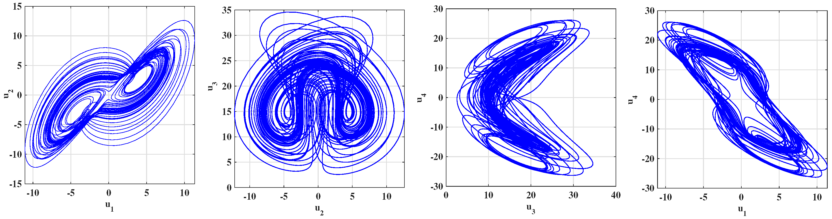
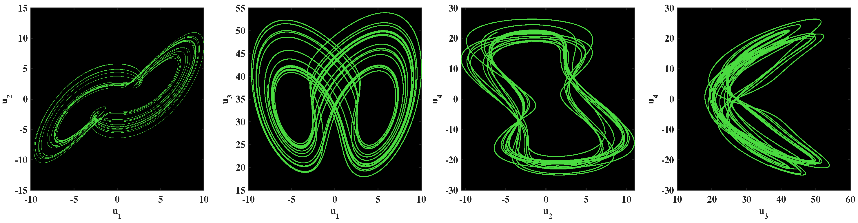
Figure 18.
Phase portraits of the chaotic system’s attractor in various 2D projections for .
Figure 18.
Phase portraits of the chaotic system’s attractor in various 2D projections for .
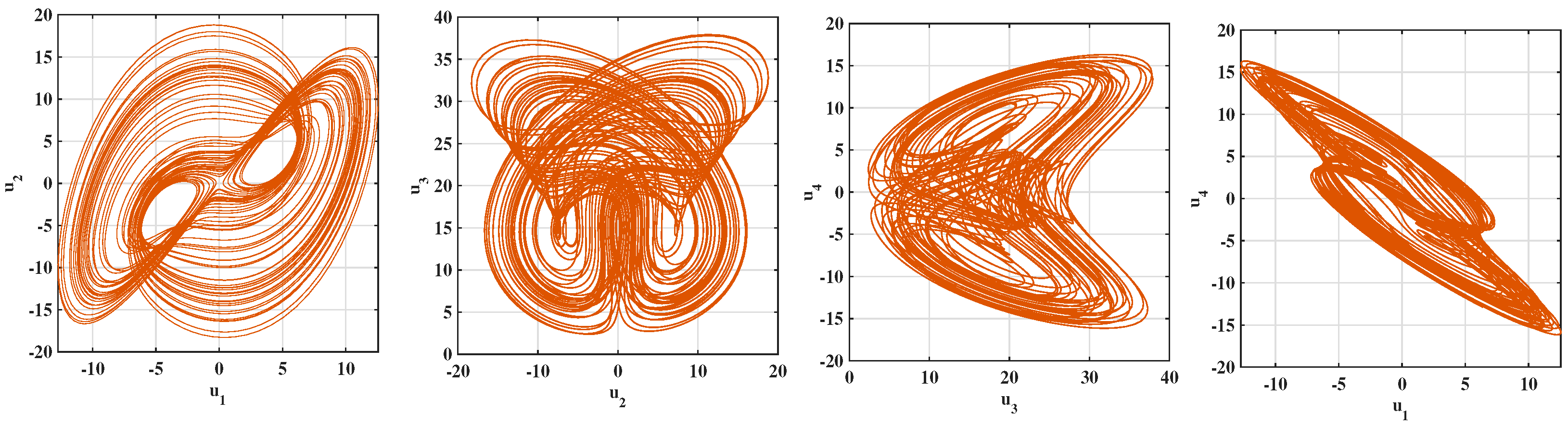
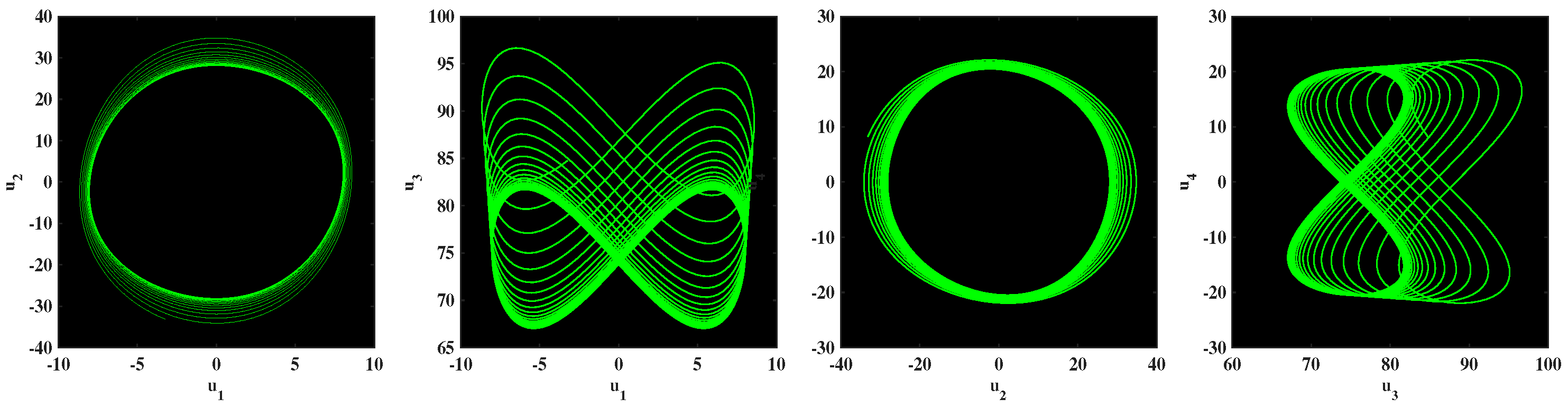
Figure 19.
Phase portraits of the chaotic system’s attractor in various 2D projections for Case 2.
Figure 19.
Phase portraits of the chaotic system’s attractor in various 2D projections for Case 2.
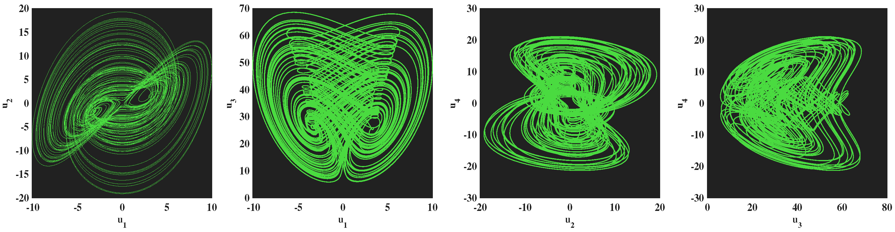
Figure 20.
Phase portraits of the chaotic system’s attractor in various 2D projections for .
Figure 20.
Phase portraits of the chaotic system’s attractor in various 2D projections for .
Figure 21.
Influence of parameter parameters: Case 1 [a = 8.2, b = 6.7, c = 4.2, d = 20]: initial condition [.
Figure 21.
Influence of parameter parameters: Case 1 [a = 8.2, b = 6.7, c = 4.2, d = 20]: initial condition [.
Figure 22.
Influence of parameter parameters: case 1 [a = 15, b = 30, c = 4,d = 15]: initial condition [.
Figure 22.
Influence of parameter parameters: case 1 [a = 15, b = 30, c = 4,d = 15]: initial condition [.
Figure 23.
Influence of parameter parameters: Case 2 [a = 15, b = 30, c = 4, d = 15]: initial condition [.
Figure 23.
Influence of parameter parameters: Case 2 [a = 15, b = 30, c = 4, d = 15]: initial condition [.
Figure 24.
Influence of parameter parameters: Case 2 [a = 7, b = 25, c = 5.8, d = 9.2]: initial condition [.
Figure 24.
Influence of parameter parameters: Case 2 [a = 7, b = 25, c = 5.8, d = 9.2]: initial condition [.
Table 1.
Comparison of analytical tools employed in related studies.
Table 1.
Comparison of analytical tools employed in related studies.
| References | FOS | VFOS | PP | ATT | NC | TSA | LE | BIF | NS |
|---|
| [24] | ✓ | ✓ | × | ✓ | ✓ | × | ✓ | ✓ | ✓ |
| [25] | ✓ | × | × | × | ✓ | × | × | ✓ | × |
| [26] | × | ✓ | × | × | ✓ | × | × | × | ✓ |
| [27] | ✓ | × | × | × | × | × | × | ✓ | × |
| [28] | × | × | × | ✓ | × | × | × | ✓ | × |
| This study | ✓ | ✓ | ✓ | ✓ | ✓ | ✓ | ✓ | ✓ | ✓ |
Table 2.
Numerical solution of Case 1: evolution of the state variables , , , and over time.
Table 2.
Numerical solution of Case 1: evolution of the state variables , , , and over time.
| Time | | | | |
|---|
| 0.0 | 0.500000 | 0.500000 | 0.600000 | 0.600000 |
| 0.1 | 0.754095 | 1.291905 | 0.531461 | −0.246540 |
| 0.2 | 1.778917 | 3.067058 | 0.695320 | −2.265370 |
| 0.3 | 4.270339 | 7.107500 | 2.179656 | −6.826865 |
| 0.4 | 9.275270 | 13.401911 | 10.227600 | −16.316005 |
| 0.5 | 12.027209 | 5.765231 | 32.494210 | −26.333870 |
| 0.6 | 1.655397 | −11.191704 | 35.881029 | −18.550057 |
| 0.7 | −4.663427 | −6.976101 | 29.213613 | −7.039850 |
| 0.8 | −3.392863 | −1.120643 | 25.979175 | −2.871681 |
| 0.9 | −0.868295 | 0.717811 | 20.844487 | −2.792647 |
| 1.0 | 0.386554 | 0.775116 | 16.154138 | −3.327416 |
Table 3.
Numerical solution for fractional order .
Table 3.
Numerical solution for fractional order .
| Time | | | | |
|---|
| 0.0 | 0.500000 | 0.500000 | 0.600000 | 0.600000 |
| 0.1 | 0.755073 | 1.293707 | 0.531449 | −0.248652 |
| 0.2 | 1.788150 | 3.082408 | 0.698393 | −2.282382 |
| 0.3 | 4.314828 | 7.176095 | 2.221502 | −6.907622 |
| 0.4 | 9.389879 | 13.474910 | 10.551691 | −16.555560 |
| 0.5 | 11.835324 | 5.042076 | 33.000107 | −26.311613 |
| 0.6 | 1.243914 | −10.999267 | 35.094549 | −17.921353 |
| 0.7 | −4.545167 | −6.559990 | 28.529128 | −6.795518 |
| 0.8 | −3.231103 | −1.206765 | 25.107785 | −2.827651 |
| 0.9 | −0.950327 | 0.414190 | 20.067335 | −2.569643 |
| 1.0 | 0.153169 | 0.492341 | 15.524089 | −2.869350 |
Table 4.
Numerical solution for Case 2: evolution of the state variables , , , and over time.
Table 4.
Numerical solution for Case 2: evolution of the state variables , , , and over time.
| Time | | | | |
|---|
| 0.0 | 0.500000 | 0.500000 | 0.600000 | 0.600000 |
| 0.1 | 0.773534 | 1.326527 | 0.531606 | −0.287267 |
| 0.2 | 1.874358 | 3.224581 | 0.729100 | −2.439326 |
| 0.3 | 4.595185 | 7.603923 | 2.498322 | −7.415171 |
| 0.4 | 9.912133 | 13.733013 | 12.149587 | −17.672065 |
| 0.5 | 10.997845 | 2.353307 | 34.593728 | −26.057164 |
| 0.6 | 0.099292 | −10.364749 | 32.885063 | −16.077085 |
| 0.7 | −4.295667 | −5.637037 | 26.840657 | −6.093761 |
| 0.8 | −2.964206 | −1.391883 | 23.194794 | −2.533065 |
| 0.9 | −1.172806 | −0.159627 | 18.490761 | −1.886375 |
| 1.0 | −0.349041 | −0.083071 | 14.322201 | −1.710400 |
Table 5.
Numerical solution for fractional order .
Table 5.
Numerical solution for fractional order .
| Time | | | | |
|---|
| 0.0 | 0.500000 | 0.500000 | 0.600000 | 0.600000 |
| 0.1 | 0.773741 | 1.326905 | 0.531606 | −0.287710 |
| 0.2 | 1.876353 | 3.227894 | 0.729814 | −2.442992 |
| 0.3 | 4.604976 | 7.618766 | 2.508359 | −7.432999 |
| 0.4 | 9.934813 | 13.740067 | 12.225960 | −17.722271 |
| 0.5 | 10.940413 | 2.202925 | 34.656304 | −26.027059 |
| 0.6 | 0.036901 | −10.299741 | 32.725490 | −15.960367 |
| 0.7 | −4.265127 | −5.572418 | 26.699303 | −6.056646 |
| 0.8 | −2.940223 | −1.415586 | 23.027247 | −2.519432 |
| 0.9 | −1.193399 | −0.217372 | 18.348897 | −1.834903 |
| 1.0 | −0.399504 | −0.147224 | 14.214947 | −1.609120 |
Table 6.
Comparison of the proposed method with the ABM method for constant fractional orders.
Table 6.
Comparison of the proposed method with the ABM method for constant fractional orders.
| Order | Time | Variable | Proposed | ABM | |Error| |
|---|
| 0.1 | | 0.755073 | 0.752673 | 0.002400 |
| | | 1.293707 | 1.219693 | 0.074014 |
| | | 0.531449 | 0.531887 | 0.000438 |
| | | −0.248652 | −0.244426 | 0.004226 |
| 0.2 | | 1.788150 | 1.778079 | 0.010071 |
| | | 3.082408 | 3.063021 | 0.019387 |
| | | 0.698393 | 0.690284 | 0.008109 |
| | | −2.282382 | −2.266205 | 0.016177 |
| 0.3 | | 4.314828 | 4.273875 | 0.040953 |
| | | 7.176095 | 7.106461 | 0.069634 |
| | | 2.221502 | 2.170537 | 0.050965 |
| | | −6.907622 | −6.823322 | 0.084300 |
| 0.4 | | 9.389879 | 9.272666 | 0.117213 |
| | | 13.474910 | 13.407635 | 0.067275 |
| | | 10.551691 | 10.387741 | 0.163950 |
| | | −16.555560 | −16.871949 | 0.316389 |
| 0.1 | | 0.773741 | 0.745655 | 0.028086 |
| | | 1.326905 | 1.459580 | 0.132675 |
| | | 0.531606 | 0.532997 | 0.001391 |
| | | −0.287710 | −0.240977 | 0.046733 |
| 0.2 | | 1.876353 | 1.070001 | 0.806352 |
| | | 3.227894 | 3.550652 | 0.322758 |
| | | 0.729814 | 0.701497 | 0.028317 |
| | | −2.442992 | −2.801010 | 0.358018 |
| 0.3 | | 4.604976 | 4.057893 | 0.547083 |
| | | 7.618766 | 7.298274 | 0.320492 |
| | | 2.508359 | 2.989400 | 0.481041 |
| | | −7.432999 | −7.263263 | 0.169736 |
| 0.4 | | 9.934813 | 9.516716 | 0.418097 |
| | | 13.740067 | 13.836564 | 0.096497 |
| | | 12.225960 | 12.292848 | 0.066888 |
| | | −17.722271 | −1.052271 | 16.670000 |
Table 7.
Comparison between the proposed variable-order method and the ABM method.
Table 7.
Comparison between the proposed variable-order method and the ABM method.
| Case | Time | Variable | Proposed | ABM | |Error| |
|---|
| Case 1 | 0.1 | | 0.754095 | 0.752673 | 0.001422 |
| | | 1.291905 | 1.219693 | 0.072212 |
| | | 0.531461 | 0.531887 | 0.000426 |
| | | −0.246540 | −0.244426 | 0.002114 |
| 0.2 | | 1.778917 | 1.778079 | 0.000838 |
| | | 3.067058 | 3.063021 | 0.004037 |
| | | 0.695320 | 0.690284 | 0.005036 |
| | | −2.265370 | −2.266205 | 0.000835 |
| 0.3 | | 4.270339 | 4.273875 | 0.003536 |
| | | 7.107500 | 7.106461 | 0.001039 |
| | | 2.179656 | 2.170537 | 0.009119 |
| | | −6.826865 | −6.823322 | 0.003543 |
| 0.4 | | 9.275270 | 9.272666 | 0.002604 |
| | | 13.401911 | 13.407635 | 0.005724 |
| | | 10.227600 | 10.387741 | 0.160141 |
| | | −16.316005 | −16.871949 | 0.555944 |
| Case 2 | 0.1 | | 0.773534 | 0.773741 | 0.000207 |
| | | 1.326527 | 1.326905 | 0.000378 |
| | | 0.531606 | 0.531606 | 0.000000 |
| | | −0.287267 | −0.287710 | 0.000443 |
| 0.2 | | 1.874358 | 1.876353 | 0.001995 |
| | | 3.224581 | 3.227894 | 0.003313 |
| | | 0.729100 | 0.729814 | 0.000714 |
| | | −2.439326 | −2.442992 | 0.003666 |
| 0.3 | | 4.595185 | 4.604976 | 0.009791 |
| | | 7.603923 | 7.618766 | 0.014843 |
| | | 2.498322 | 2.508359 | 0.010037 |
| | | −7.415171 | −7.432999 | 0.017828 |
| 0.4 | | 9.912133 | 9.934813 | 0.022680 |
| | | 13.733013 | 13.740067 | 0.007054 |
| | | 12.149587 | 12.225960 | 0.076373 |
| | | −17.672065 | −17.722271 | 0.050206 |