Article

Fuzzy Comprehensive Evaluation of the Geological Environment of Abandoned Open-Pit Mines Based on IRBMO-G1-EWM Combined Weighting


School of Civil Engineering, Central South University, Railway Campus, No. 22, Shaoshan South Rd., Changsha 410075, China
*
Author to whom correspondence should be addressed.
Mathematics 2026, 14(13), 2448; https://doi.org/10.3390/math14132448
Submission received: 16 April 2026 / Revised: 14 June 2026 / Accepted: 27 June 2026 / Published: 7 July 2026
(This article belongs to the Special Issue Sensitivity Analysis and Decision Making)

Abstract

The geological environment evaluation of abandoned open-pit mines frequently encounters challenges, including the reliance of subjective weighting on judgment matrices, the complexity of weight adjustment, and the inadequate interpretation of systematic evaluation results. Addressing these limitations in existing AHP/FAHP and their combinatory weighting models, this study proposes the IRBMO-G1-EWM-FCE framework. This framework embeds the Improved Red Billed Blue Magpie Optimizer (IRBMO) into the improved G1 method to optimize indicator contribution rates, and subsequently integrates EWM, game theory combinatory weighting, and Fuzzy Comprehensive Evaluation (FCE) to evaluate three abandoned quarries in the Yellow River Basin of Shaanxi Province. The results demonstrate that across 20 independent runs, IRBMO yields a mean fitness value of 1.6496, lower than the 1.7732 of RBMO, with a 63.8% reduction in standard deviation, thereby indicating superior convergence accuracy and stability. The comprehensive membership degrees of the three quarries are A = [0.405,0.143,0.452], B = [0.405,0.450,0.145], and C = [0.742,0.077,0.181], corresponding to evaluation grades of Grade III, Grade II, and Grade I, respectively. While circumventing the construction of complete judgment matrices and consistency modifications, this method incorporates both expert experience and data discreteness into the evaluation, thereby providing an interpretable quantitative tool for geological environment classification, governance priority identification, and restoration decision-making for abandoned open-pit mines.

1. Introduction

Mining activities serve as the fundamental basis for global industrial development; however, the resultant abandoned open-pit mines pose severe threats to ecological stability and geological safety. Improper exploitation and utilization of mineral resources have led to a large number of abandoned open-pit mines. These mines are typically characterized by high and steep slopes, fractured rock masses, and degraded vegetation, resulting in elevated risks of landslides and debris flows [1,2,3,4,5,6,7]. Consequently, the scientific and quantitative evaluation of the ecological geological environment constitutes a prerequisite for effective mine restoration [8]. Extensive research has been conducted by scholars on the geological environment evaluation of abandoned open-pit mines. Qi et al. [9] selected evaluation indicators by employing DInSAR technology to quantify the impact of mining activities on the surface of coal mining areas. They combined the Analytic Hierarchy Process (AHP) and the Entropy Weight Method (EWM) to calculate indicator weights, thereby constructing a novel evaluation model for the mine geological environment. Sun et al. [10] integrated Principal Component Analysis (PCA) with catastrophe theory, proposing a new method for evaluating the mine ecological geological environment. Zhu et al. [11] merged the AHP-CRITIC coupled weighting model with the multi-scale geographically weighted regression (MGWR) model to establish a Landscape Ecological Quality Regulation evaluation framework for coal mining areas characterized by a high degree of landscape fragmentation. Wu et al. [12] developed a mine geological environment quality evaluation system by combining the Analytic Network Process (ANP) with the Coefficient of Variation (CV) weighting method, utilizing Geographic Information System (GIS) technology. Guo et al. [13] proposed a new abandoned open-pit mine geological environment information system (MGEIS), and utilized it to evaluate the geological environment of abandoned open-pit mines in Jilin Province, China.
The ecological geological environment evaluation of abandoned open-pit mines is essentially a multi-criteria decision-making problem characterized by high uncertainty, fuzziness, and complexity [14]. Although numerous MCDM and fuzzy evaluation models have been applied to the domain of mine geological environment assessment, several limitations persist. The AHP-EWM model integrates expert judgment with data-driven information; however, AHP relies on judgment matrices and consistency checks [15]. When numerous indicators are involved, the construction and adjustment of judgment matrices become exceedingly cumbersome, while subjective inconsistency may still compromise the determination of final weights. The ANP-CV model can delineate the interrelationships among indicators and reflect data variability; nevertheless, ANP necessitates the construction of complex network structures and extensive expert comparisons, whereas CV is exceedingly sensitive to the dispersion of anomalous data. Models based on the CRITIC method can gauge contrast intensity and conflict among indicators, yet these approaches predominantly rely on statistical variation and correlation, potentially undermining the expert comprehension of geological mechanisms. Weighting models based on PSO or other metaheuristic methods optimize the weight search process; however, many of these models treat the optimization algorithm merely as a surrogate tool, failing to explicitly elucidate the specific weighting mechanism being optimized or to demonstrate whether the derived weights genuinely enhance the ultimate evaluation grade. Although comprehensive weighting models based on metaheuristic optimization methods have been extensively reported [16,17,18,19,20,21,22,23,24,25,26], the subjective weighting mechanism within these models conventionally inherits from AHP, FAHP, or analogous pairwise comparison methodologies. In contrast, this study focuses on a disparate weighting mechanism. The improved G1 method circumvents the procedure of constructing a complete one-to-one judgment matrix, instead manifesting expert knowledge through an ordered importance sequence and adjacent importance ratios. However, upon the introduction of indicator contribution rates, the improved G1 method [27] engenders a nonlinear constrained optimization problem. Consequently, the Improved Red Billed Blue Magpie Optimizer (IRBMO) is selected as the fundamental optimizer because its search, storage, and update mechanisms facilitate a flexible equilibrium between global exploration and local exploitation. By incorporating circle chaotic mapping to augment the population diversity of the RBMO algorithm and integrating Cauchy mutation to elevate the capability of the algorithm to escape local optima, this algorithm is highly suitable for addressing this category of nonlinear constrained optimization problems. IRBMO is not merely utilized as an alternative to PSO, GWO, or WOA; rather, it serves as a targeted optimizer for the contribution rate estimation problem within the improved G1 weighting mechanism. This study integrates the subjective weights derived from IRBMO-G1 with the objective weights derived from EWM, proposing a geological environment evaluation method for abandoned open-pit mines based on Fuzzy Comprehensive Evaluation (FCE). In comparison with extant models, the proposed IRBMO-G1-EWM-FCE model retains expert interpretability via the G1 ranking mechanism while circumventing the cumbersome judgment matrix construction process necessitated by AHP or FAHP. Furthermore, it utilizes IRBMO to optimize contribution rates within the improved G1 method, thereby mitigating the subjective arbitrariness inherent in subjective weighting. It amalgamates the optimized subjective weights with the objective weights deduced from EWM and the FCE classification, enabling both geological expert knowledge and data dispersion to be manifested in the ultimate assessment.
It is noteworthy that the previous study by the author [28] also focused on the geological environment evaluation of abandoned open-pit mines and adopted evaluation procedures including EWM, combination weighting, and FCE. Therefore, the research focus of this paper is not to propose a completely novel fuzzy comprehensive evaluation framework, but to implement algorithmic improvements and methodological integration for the pivotal subjective weighting procedure within the evaluation model. Compared with the previous study, although this paper still designates the ecological restoration demonstration engineering area of the Yellow River Basin in Shaanxi Province as the study area, the evaluation objects are not the identical engineering cases from the previous study, but rather different abandoned quarries selected for evaluation and analysis within the same study area context. This approach facilitates further investigation into the effects of different subjective weighting mechanisms on the final weights, membership degree vectors, and evaluation grades under analogous regional geological backgrounds, ecological restoration objectives, and management contexts. Distinct from the IRMO-FAHP model, this paper does not adopt the fuzzy pairwise comparison matrix in FAHP, nor does it consider the consistency modification of the judgment matrix as the optimization objective. Instead, it embeds the Improved Red-billed Blue Magpie Optimizer (IRBMO) into the improved G1 method, utilizing indicator importance ranking and adjacent importance ratios provided by experts to optimize indicator contribution rates under weak consistency constraints. Consequently, substantial differences exist between this paper and the previous study regarding modes of subjective judgment expression, optimization variables, objective functions, constraint conditions, and weight generation pathways. The previous study primarily addressed the consistency improvement issue of the FAHP fuzzy judgment matrix, whereas this paper focuses on optimizing the indicator contribution rates within the improved G1 method, and further analyzes the effects of this subjective weighting mechanism on the combination weights, membership degree vectors, and final evaluation grades.
The ecological restoration demonstration project area in the Yellow River Basin in Shaanxi Province is selected as the study area, as it constitutes a pivotal ecological restoration zone characterized by the ubiquitous distribution of abandoned open-pit quarries, where geological hazard prevention, soil erosion control, and land reclamation represent imperative management tasks demanding urgent resolution. Although the formulated indicator system is designed for universal applicability to abandoned open-pit mines, the current empirical validation remains region-specific. Consequently, whether the applicability of this model can be extrapolated to other geological and climatic regions necessitates further validation utilizing more extensive datasets. As this case study encompasses merely three queries, the objective weights derived from EWM may be susceptible to data dispersion and therefore should not be construed as universally stable statistical weights. In the present study, EWM serves as a data-driven modification mechanism to calibrate the subjective weights assigned by experts. The magnitude of its influence will be further investigated through sensitivity and comparative analyses.
Overall, this study emphasizes the improvement of the subjective weight generation process and validates its impact on system-level evaluation outcomes. The integration of expert knowledge, objective data characteristics, and fuzzy evaluation methodologies provides a practicable approach for evaluating the geological environment of abandoned open-pit mines. The contributions of this study are as follows:
(1)
The RBMO algorithm is improved by incorporating Circle chaotic mapping and Cauchy mutation to augment the population diversity and local optima evasion capability of the algorithm.
(2)
The IRBMO algorithm is embedded into the improved G1 method to propose the IRBMO-G1 subjective weighting method, which is utilized to optimize indicator contribution rates under weak consistency constraints, thereby mitigating the arbitrariness inherent in subjective weighting.
(3)
The IRBMO-G1 subjective weights, EWM objective weights, game theory combinatory weighting, and FCE are integrated and applied to three quarries in the Yellow River Basin of Shaanxi Province; concurrently, the interpretability and robustness of the results are verified through alternative evaluation method comparisons and sensitivity analyses of the subjective weights

2. Construction of the Geological Environment Evaluation Index System for Abandoned Open-Pit Mines

2.1. Selection of Evaluation Index

The geological environment of abandoned open-pit mines is governed by numerous evaluation factors, wherein various evaluation indices exert differential degrees of influence. Adhering to the principles of systematicity, dynamics, scientificity, and universality, and drawing upon the existing literature [28,29,30,31,32,33,34,35,36,37,38,39,40,41,42,43,44,45], this study constructs an evaluation index system for the geological environment of abandoned open-pit mines across three dimensions: geological conditions, resource damage, and geological environment problems. This system comprises three criteria layers encompassing geological conditions, resource damage, and geological environment problems, along with thirteen index layers. The specifics are detailed in Table 1.
The evaluation index system for the geological environment of abandoned open-pit mines in this study predominantly comprises three major categories: the geological background conditions of the mines, the degree of resource and environmental damage induced by mining activities, and the subsequent geological disasters and environmental problems. Regarding geological conditions, the system incorporates indices including rock type, hydrogeological conditions, topography and geomorphology, seismic intensity, and geological structure, which collectively dictate the intrinsic sensitivity and stability of the mine’s geological environment. Concerning the aspect of resource damage, parameters such as land destruction area, exposed rock-face ratio, degree of aquifer destruction, and landscape destruction ratio are utilized to elucidate the tangible impacts of mining on land, water resources, and ecological landscapes. In the context of geological disasters and environmental problems, emphasis is placed on the comprehensive soil and water pollution degree, the scale and quantity of geological disasters, and soil erosion conditions. These indices aptly reflect the secondary environmental risks confronting abandoned mines and the urgency of their subsequent remediation.
To further elucidate the relationship between the proposed index system and the previous study by the authors [28], an item-by-item comparison of the evaluation indicators employed in both studies was conducted, with the results presented in Table 2. As both studies target the geological environment evaluation of abandoned open-pit mines, a certain degree of overlap exists in fundamental evaluation dimensions, including hydrogeological conditions, topography and geomorphology, seismic intensity, land damage, aquifer destruction, water and soil pollution, and soil erosion. Such indicators are commonly utilized and indispensable fundamental indicators in the geological environment evaluation of abandoned open-pit mines; their overlap primarily reflects the consistency of the evaluation objects rather than constituting mere duplication of the previous study. Compared with [28], the present study does not directly adopt the original indicator system; instead, it reorganizes and refines the indicator framework in accordance with the geological environment characteristics and evaluation objectives of the current research objects. For instance, lithology and geological structure are incorporated into the evaluation system as independent indicators to more directly reflect the impacts of rock mass stability and structural plane development on the mine geological environment; the proportion of exposed rock surfaces is introduced to characterize the exposed rock walls of abandoned quarries, the difficulty of ecological revegetation, and the degree of landscape destruction; meanwhile, the relatively broad indicators from the previous study are further disaggregated. Consequently, the distinctions between the present study and [28] manifest not only in the research objects and data sources but also in the structural adjustment of the index system and the mode of expressing evaluation information.
As indicated in Table 2, overlaps exist between the present study and [28] regarding certain fundamental indices. However, these indices predominantly pertain to universal fundamental dimensions within the geological environment evaluation of abandoned open-pit mines, and their retention ensures the completeness and comparability of the evaluation system. In accordance with the geological environment characteristics of the current research objects, significant adjustments were made to the index system in the present study. On the one hand, lithology and geological structure were isolated from the broad category of engineering geological conditions to enhance the representation of rock mass stability and structural plane development characteristics. On the other hand, the proportion of exposed rock surfaces was introduced, and geological hazards were further decomposed into hazard scale and hazard quantity to respectively reflect the revegetation difficulty of exposed rock walls in quarries, hazard intensity, and hazard occurrence frequency. Consequently, the index system of the present study does not constitute a mere duplication of [28]; rather, it represents a reconstruction and refinement tailored to the geological environment characteristics of abandoned quarries, built upon the shared fundamental evaluation dimensions. The novelty of the present study is primarily embodied in the reorganization of the index system, the utilization of distinct case data, and the optimization of index contribution rates through the subjective weighting mechanism of IRBMO-G1, rather than claiming that every evaluation index is entirely novel.

2.2. Independence of Evaluation Indicators and Rationality of Classification Thresholds

Given that the evaluation indices encompass both qualitative (QL) and quantitative (QN) categories characterized by disparate classification criteria, this study establishes a uniform and comprehensive evaluation standard for the geological environment of abandoned open-pit mines based on literature [33,46,47,48,49] to standardize these criteria. All indices are uniformly classified into three grades: slight, moderate, and severe. The classification criteria are established through a comprehensive synthesis of relevant technical specifications, extant research on mine geological environment evaluation, field investigation data from the study area, and expert judgment. The specific classification criteria are presented in Table 3.
To enhance the reproducibility of qualitative index assignment, this study further refines the three-level discrimination criteria for qualitative indices, including A1, A2, A3, A5, B3, and C4. Distinct from the mere utilization of generalized descriptions such as “slight, moderate, and severe”, this study assigns values to qualitative indices based on observable characteristics including lithological weathering, joint and fissure development, groundwater disturbance, topographic relief, structural complexity, the influence range of aquifer destruction, and soil erosion patterns, by integrating field investigations, engineering geological data, and mine geological environment evaluation experience. The specific operational discrimination criteria are presented in Table 4.
Table 5 presents the threshold sources and classification criteria for each index. For indices with explicit normative foundations, relevant technical standards are prioritized; conversely, indices lacking unified national standards are determined by integrating extant research on mine geological environment evaluation, field investigation data from the study area, and expert judgment. As delineated in Table 5, indices such as C1, C2, C3, and C4 possess relatively explicit normative or investigative bases, whereas indices such as B2 and B4, owing to the absence of unified national classification thresholds, are primarily determined by synthesizing extant research and the actual conditions of the study area. It is imperative to note that certain thresholds exhibit regional applicability; consequently, when this evaluation framework is extrapolated to other mine types or disparate geomorphological and climatic regions, adjustments should be implemented in accordance with local geological environment contexts and restoration objectives.
To further elucidate the absence of conspicuous redundancy within the index system, this study compares index pairs exhibiting potential conceptual correlations, with a focused analysis on three dimensions: measurement objects, geological implications, and governance management significance. Although these indicators are uniformly associated with the deterioration of the mine’s geological environment, they respectively delineate disparate risk dimensions, thereby exhibiting complementarity rather than substitutability, as detailed in Table 6.
P z = max C 1 C o 2 + C 1 C o ¯ 2 2
The calculation formula for Pz is expressed as Equation (1), where C1 denotes the measured concentration of a specific pollutant in a point sample of surface water, groundwater, or soil, and C0 denotes the limit value for a specific pollutant stipulated in the national standards for surface water, groundwater, or soil.
As demonstrated in Table 6, potentially correlated indices exhibit distinct disparities regarding measurement objects and governance implications. The retention of these indices facilitates the differentiation of hazard intensity, hazard occurrence frequency, land reclamation engineering volume, degree of landscape disturbance, and difficulty of ecological restoration during the evaluation process, thereby enhancing the explanatory power of the evaluation outcomes for subsequent governance and restoration decisions.

3. Combined Weight Determination Method Based on IRBMO-G1-EWM

3.1. IRBMO-G1 Algorithm for Optimal Subjective Weight Determination

3.1.1. The Improved G1 Method

Building upon the G1 method, the improved G1 method is a novel subjective weight determination approach proposed by incorporating the probability of evaluation index contribution rates. The improved G1 method, which integrates the evaluation index contribution rates, places greater emphasis on weak consistency, thereby overcoming the discrepancy between the numerical assignment of evaluation indices and actual human cognitive processes [50]. The specific procedures are given as follows:
(1)
Determination of the order relation.
Based on empirical expertise, experts rank the index set {x1, x2, …, xn} according to their degrees of importance to derive a new sequence denoted as A1 > A2 > … > An.
(2)
Rational assignment.
Based on geological environment evaluation experience, experts determine the ranking relationship of index contribution degrees and assign values to the contribution degrees of adjacent indices, denoted as rk. rk signifies the ratio of the contribution degree of the (j − 1)th index to that of the jth index subsequent to ranking. The value range of rk can be referenced in Table 7.
(3)
Incorporation of the evaluation index contribution rate cj.
The original data matrix X = (xij)m×n undergoes standardization via Equation (2), categorizing the index into a positive index (where larger values are preferable) and a negative index.
Positive   index   :   z i j = x i j x j max Negative   index   :   z i j = x j min x i j
where zij represents the value of the j-th evaluation index following standardization, and xjmax and xjmin denote the maximum and minimum values of the j-th index prior to standardization, respectively. Rearranging the standardized data matrix according to the order relation yields matrix A = (aij)m×n. The calculation formula for the evaluation index contribution rate is delineated in Equation (3).
c j = w j   i = 1 m a i j / j = 1 n i = 1 m w j a i j    
where cj denotes the contribution rate of the jth-ranked index, wj represents its subjective weight, and aij signifies the standardized value of the ith evaluation object with respect to the jth-ranked index.
The contribution rate is not exclusively an outcome of expert judgment; rather, it is jointly determined by index weights and the empirical data of evaluation objects. cj reflects the proportion of a specific index within the comprehensive evaluation values across all evaluation objects, thereby coupling expert judgment with the empirical data of the study area to a certain extent.
(4)
Formulate the objective function f and compute the subjective weights.
Following the determination of rk, the improved G1 method eschews the direct sequential multiplication of rk to derive indicator weights; rather, it initially constructs an optimization model utilizing the index contribution rate c = (c1, c2, …, cn) as the decision variable. The objective of this model is to ensure the ratio of adjacent index contribution rates, cj − 1/cj, approximates the adjacent contribution degree ratio rk assigned by experts as closely as possible, while concurrently guaranteeing that the contribution rate sequence satisfies the expert ranking relationship and weak consistency constraints. The specific optimization model is formulated as follows:
min f = j = 2 n ( c j 1 c j r k ) 2 s . t . c j 1 r k c j 0 , j = 2 , 3 , , n c j c j 1 0 , j = 2 , 3 , , n c 1 1.8 c n 0 j = 1 n c j = 1
In the equations, the objective function f quantifies the deviation between the ratio of adjacent index contribution rates and the expert judgment value rk. A smaller f signifies that the contribution rate sequence more closely conforms to the expert judgment regarding the contribution degrees of adjacent indices. The constraint cj − 1 − rkcj ≤ 0 dictates that the discrepancy between adjacent index contribution rates does not exceed the contribution degree ratio specified by experts, while the constraint cjcj − 1 ≤ 0 ensures that the contribution rate of a preceding ranked indicator is no less than that of a succeeding one, thereby preserving the index importance sequence determined by experts. These two constraints collectively embody the weak consistency requirement. The constraint c1 − 1.8cn ≤ 0 serves to restrict the overall disparity between the contribution rates of the first and last indices, precluding the excessive amplification of contribution rate discrepancies arising from the sequential multiplication of adjacent ratios under strong consistency conditions, and the constraint ∑cj = 1 guarantees that all index contribution rates constitute a normalized proportion.
Equation (4) yields the optimal index contribution rate vector c = (c1, c2, …, cn) satisfying the expert ranking relationship, adjacent contribution degree judgments, and weak consistency constraints. However, the contribution rate is not equivalent to the final subjective weight. As indicated by Equation (3), the contribution rate cj is simultaneously influenced by the index weight wj and the cumulative standardized value lj of the respective index across all evaluation objects. Consequently, upon obtaining the optimal contribution rate, the subjective weights of the ranked indices must be derived inversely based on the relationship between the contribution rates and the cumulative standardized values. The calculation procedure is expressed as Equation (5).
w n = 1 + l n c n j = 2 n c j 1 l j 1 1 , l j = i = 1 m a i j w j 1 = w j l j c j 1 c j l j 1 , j = n , , 3 , 2
where lj denotes the sum of standardized values of the jth ranked evaluation index across m evaluation objects, representing the cumulative performance value of the index within the research sample.
Through Equation (5), the subjective weights of the indices can be calculated according to the ordinal relation A, and subsequently converted into the subjective weights of the original evaluation indices corresponding to the index set, expressed as w = (w1, w2, …, wn).

3.1.2. IRBMO Algorithm

  • RBMO
In 2024, Fu et al. [51] proposed a novel metaheuristic algorithm termed the Red-billed Blue Magpie Optimization (RBMO) algorithm. By simulating the searching, chasing, and attacking, and food storing behaviors of the red-billed blue magpie, the mathematical model of RBMO was formulated, featuring minimal parameters, operational simplicity, and robust local exploitation capability. Based on the characteristics of the red-billed blue magpie, the predation process is partitioned into three phases: food searching, food attacking, and food storing. The procedural steps of the RBMO algorithm are delineated as follows:
  • (1)
    Generate the initial population
Assuming n red-billed blue magpies engage in predation within a space of nod dimensions, their positions can be formulated as Equation (6):
X = X 1 , 1 X 1 , 2 X 1 , n o d X 2 , 1 X 2 , 2 X 2 , n o d X n , 1 X n , 2 X n , n o d
where i denotes the i-th bird within the flock, j signifies the j-th dimension of the problem to be solved, and X is computed as delineated in Equation (7).
X i , j = ( u b l b ) R a n d + l b
where ub and lb denote the upper and lower bounds of the problem to be solved, respectively, and Rand signifies a random number uniformly distributed over the interval (0, 1).
  • (2)
    Foraging Phase
During predation, to enhance search efficiency, red-billed blue magpies typically forage in small groups (2 to 5 individuals) or large flocks (exceeding 10 individuals). When adopting the small-group mode, position updating is executed utilizing Equation (8):
X i ( t + 1 ) = X i ( t ) + 1 p m = 1 p X m ( t ) X r s ( t ) R a n d
where t denotes the iteration count, and Xi(t + 1) signifies the new position of the i-th bird. Additionally, p is an integer ranging from 2 to 5, representing the number of individuals randomly selected from the flock for small-group searching. Furthermore, Xm denotes the m-th bird within the selected group, Xi represents the i-th individual within the flock, and Xrs(t) indicates the randomly selected individual at the t-th iteration. When foraging in the large flock mode, position updating is executed utilizing Equation (9):
X i ( t + 1 ) = X i ( t ) + 1 q m = 1 q X m ( t ) X r s ( t ) R a n d
where q denotes an integer ranging from 10 to n, representing the number of individuals randomly selected from the flock to conduct flock-based searching.
  • (3)
    Food Attacking Phase
During small-group hunting, the primary targets generally comprise plants or small prey. The corresponding mathematical models are formulated as Equations (10) and (11):
X i ( t + 1 ) = X f o o d ( t ) + C F 1 p m = 1 p X m ( t ) X i ( t ) R a n d n
C F = 1 t / T ( 2 t / T )
where t denotes the current iteration count, and T signifies the maximum iteration limit. Furthermore, Xfood(t) represents the food position, while Randn designates a random number drawn from a standard normal distribution. When hunting in flocks, they are capable of cooperatively attacking larger prey, in which case Equation (12) is utilized to execute the iteration.
X i ( t + 1 ) = X f o o d ( t ) + C F 1 q m = 1 q X m ( t ) X i ( t ) R a n d n
  • (4)
    Food Storage Phase
Following foraging and attacking food, red-billed blue magpies store surplus food in concealed locations to ensure a stable food supply. This behavior enables the algorithm to preserve the positions of historical target solutions during the iteration process, thereby enhancing the probability of attaining the global optimum. The corresponding mathematical model is formulated as follows:
X i t + 1 = X i t , f i t n e s s o l d i < f i t n e s s n e w i X i t + 1 , e l s e
where fitnessiold and fitnessinew respectively denote the fitness function values of the i-th red-billed blue magpie prior to and subsequent to its position update.
b.
Improvement of RBMO
RBMO addresses problems and executes optimization utilizing a search, storage, exploitation, and storage structure [52]. However, the search phase exhibits an over-reliance on the guidance of the optimal individual, which readily induces a rapid degradation of population diversity and predisposes the algorithm to local optima. Consequently, this study incorporates the Circle chaotic mapping strategy to augment population diversity, thereby broadening the search scope. Furthermore, Cauchy mutation perturbation is integrated into the iterative updating process to mitigate susceptibility to local optima during the late convergence stage, ultimately enhancing the quality of the optimal solution.
  • (1)
    Initialization via Circle Chaotic Mapping
In the RBMO algorithm, the initial population positions are randomly generated, which potentially results in an uneven distribution of individuals and subsequently impairs the search capability. As a quintessential chaotic mapping, the Circle mapping ensures a uniform distribution of the population within constraint boundaries and possesses high ergodicity, enabling the algorithm to explore the entire search space more efficiently. Therefore, the Circle mapping is employed during the population initialization phase to stochastically generate the initial population, as delineated by Equation (14):
X k + 1 = mod X k + 0.2 0.5 2 π sin ( 2 π X k ) , 1
where Xk denotes the initially generated random population, and Xk+1 represents the population subsequent to mapping.
This study selects the Circle chaotic map primarily owing to its excellent ergodicity, aperiodicity, and sensitivity to initial values, enabling the generation of a relatively dispersed initial population within the search space, thereby augmenting the early global exploration capability of the algorithm. Compared with conventional chaotic maps such as Logistic, Tent, Sinusoidal, and Bernoulli, the Circle map exhibits a relatively smooth state transition process while preserving stochastic perturbation characteristics, rendering it more appropriate for population initialization in the low-dimensional continuous weight optimization problem of the present study.
  • (2)
    Cauchy Mutation Strategy
During the later stages of iteration, the RBMO algorithm is susceptible to falling into local optima, thereby failing to converge to the theoretical optimum. To address this issue, the Cauchy mutation perturbation is introduced to ameliorate the population during the late iteration phase. The Cauchy mutation strategy facilitates substantial jumps within the solution space, effectively assisting individuals in escaping local optima. The mathematical formulation of the Cauchy mutation perturbation is expressed as Equation (15).
X ( t ) = X f o o d ( t ) 1 + C a u c h y ( 0 , 1 ) f ( x ) = 1 π ( 1 + x 2 ) , < x < +
where f(x) denotes the probability density function of the Cauchy distribution, X(t) signifies the perturbed position, and the remaining term represents a random number drawn from the standard Cauchy distribution.

3.1.3. Benchmark Function Validation of IRBMO

This study employs the CEC2017 standard benchmark function suite to test the IRBMO algorithm. The CEC2017 function suite encompasses unimodal, multimodal, hybrid, and composite functions, facilitating a comprehensive examination of optimization algorithm performance regarding global search capability, local exploitation capability, and the capacity to escape local optima. Hippopotamus Optimization algorithm (HO), Gray Wolf Optimization algorithm (GWO), Whale Optimization algorithm (WO), RBMO, and IRBMO are selected as comparative algorithms, uniformly configured with a population size of n = 30, a maximum iteration count of T = 10,000, and a variable dimension of dim = 30. Each function undergoes 30 independent runs, with the mean, standard deviation, and optimum of the optimal fitness values statistically analyzed to assess the optimization accuracy and stability of the respective algorithms. Partial test results are presented in Table 8, and typical convergence curves are illustrated in Figure 1.
As indicated by Table 8, IRBMO attains superior optimization results on the majority of test functions. For the unimodal function F1, both IRBMO and RBMO converge in proximity to the theoretical optimum with negligible standard deviations, demonstrating their robust local exploitation capabilities on unimodal functions. In contrast, the Mean fitness values of GWO, HO, and WOA are significantly higher, indicating their deficient convergence precision on this function. Regarding the simple multimodal function F5, the Best and Mean values of IRBMO are the lowest among the five algorithms, and its standard deviation is also smaller than those of RBMO, GWO, and WOA, signifying that the Circle chaotic map and Cauchy mutation strategy can enhance the global search capability of the algorithm and diminish the probability of entrapment in local optima. For the hybrid function F20, IRBMO secures the lowest Best value, indicating its robust optimization potential in complex search spaces, concurrently exhibiting the minimum standard deviation. Concerning the composite function F26, IRBMO yields the lowest Mean value, demonstrating its commendable search performance even in complex functions characterized by pronounced multimodal, nonlinear, and composite features. Although HO and WOA attain lower Best values in isolated runs, their execution results exhibit substantial fluctuations, manifesting insufficient stability.
Figure 1 further illustrates the average convergence process of various algorithms over 30 independent runs on representative CEC2017 functions. IRBMO exhibits a rapid convergence rate on all four test functions and sustains lower objective function values during the later iterative phases. In F5 and F26, IRBMO transitions into the stable convergence phase earlier, with its ultimate objective function value remaining lower than those of most comparative algorithms. Overall, the CEC2017 benchmark function test results indicate that IRBMO demonstrates superior search precision, convergence rate, and stability in standard continuous optimization problems.

3.1.4. IRBMO-G1 Algorithm

The improved G1 method necessitates determining the contribution rates of evaluation indices to derive optimal subjective weights, and calculating these contribution rates essentially constitutes an optimization process for the objective function. Accordingly, this study introduces the IRBMO algorithm to optimize the objective function of the improved G1 method, thereby improving the weak consistency and data adaptability of the derived subjective weights. In the IRBMO-G1 algorithm, each particle represents the contribution rate vector for the evaluation indices, where a smaller fitness value indicates that the adjacent contribution rates among indices more closely approximate the importance ratios stipulated by experts. The weak consistency constraint ensures that the optimized contribution rates preserve the expert ranking order, thereby precluding unreasonable dominant relationships among indices. Contribution rates are jointly defined based on subjective weights and standardized evaluation data; the optimized contribution rate vector reflects not only expert preference information but also the actual data distribution of the indices. Upon acquiring the optimal contribution rates, Equation (5) maps them onto the corresponding subjective weights. The derived subjective weights can be regarded as optimized, as they mitigate deviations from adjacent importance judgments of experts, satisfy weak consistency, and incorporate standardized data information, rather than relying exclusively on direct subjective assignment.
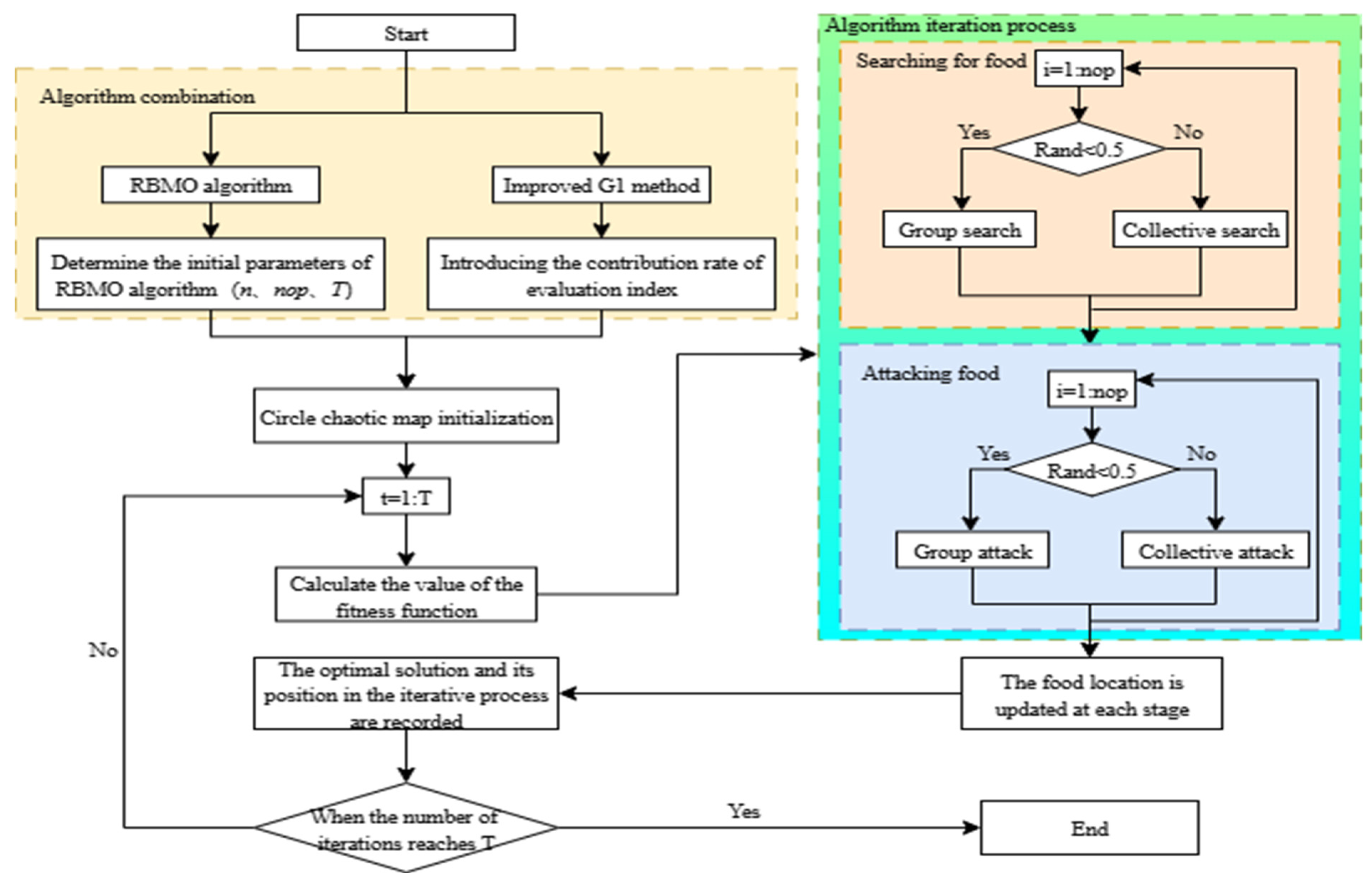
Based on the number of evaluation indices, a particle information matrix C storing nop n-dimensional particles is established as expressed in Equation (16), utilizing the objective function of Equation (4) as the fitness function of the algorithm. By evaluating the fitness function, the index contribution rates are updated through comparisons of fitness values during the iteration process. The ultimate outcome, namely the optimal evaluation index contribution rates, is determined by the optimal fitness value. The computational procedure for deriving the optimal evaluation index contribution rates via the IRBMO-G1 method is illustrated in Figure 2.
C = c 1 1 c 2 1 c n 1 c 1 2 c 2 2 c n 2 c 1 n o p c 2 n o p c n n o p

3.2. Comparative Verification Analysis of the IRBMO-G1 Algorithm

3.2.1. Analysis of Algorithm Computational Complexity and Runtime Efficiency

To evaluate the computational efficiency of the IRBMO algorithm, this study utilizes the numerical example from reference [53] as a basis, employing the HO, GWO, WO, RBMO, and IRBMO algorithms, respectively, to solve the contribution rates of the evaluation indices, with the analysis conducted from the two aspects of theoretical computational complexity and actual execution time. All algorithms employ identical parameter settings: the optimization variables are defined as the contribution rate vector c = (c1, c2, …, cn), with variable boundaries set to 0 < cj < 1, a population size N of 100, a maximum iteration count T of 50, and a dimension of variables to be optimized D of 16. All algorithms terminate upon attaining the maximum iteration count. Assuming the computational complexity of a single fitness function evaluation is O(F), the primary computational procedures of swarm intelligence optimization algorithms encompass population initialization, individual position updating, and fitness function evaluation. Specifically, the computational complexity of population initialization is O(ND), that of position updating per iteration is O(ND), and that of fitness function evaluation is O(NF). Consequently, the overall time complexity of the algorithm can be expressed as
O ( N D ) + O [ T ( N D + N F ) ]
In the improved G1 subjective weighting optimization problem addressed in this study, the fitness function primarily involves the contribution rates of indices, adjacent importance ratios, weight computation, and the assessment of weak consistency constraints. Its computational cost exhibits an approximately linear relationship with the dimension of optimization variables, namely F = O(D). Therefore, the time complexity of the algorithm within the application scenario of this study can be further simplified as
O ( T N D )
Under the parameter configurations of this study, each independent run of every algorithm necessitates approximately N × T = 100 × 50 = 5000 optimal solution updates and fitness function evaluations. Given the optimization variable dimension of D = 16, this weight optimization problem constitutes a low-dimensional optimization problem. Consequently, all algorithms can accomplish the computation within a brief duration. Building upon RBMO, IRBMO incorporates the Circle chaotic map and the Cauchy mutation strategy. The Circle chaotic map is primarily utilized during the initialization phase to enhance population distribution uniformity, incurring a computational complexity of O(ND), whereas the Cauchy mutation strategy operates during the iterative update phase, also with a computational complexity of O(ND). Although these improvement strategies introduce a certain constant-level computational overhead, they do not alter the order of magnitude of the overall algorithmic complexity. Therefore, the theoretical time complexity of IRBMO remains O(TND). Regarding space complexity, IRBMO primarily necessitates the storage of the population position matrix, fitness values, and the current optimal individual, with the population position matrix occupying the predominant portion, resulting in a space complexity of O(ND).
As demonstrated in Table 9, under identical parameter configurations and operating environments, all five algorithms exhibit theoretical time complexity of O(TND) and space complexity of O(ND). This indicates that incorporating the Circle chaotic map and the Cauchy mutation strategy into RBMO to derive IRBMO does not alter the order of magnitude of the overall algorithmic complexity. Regarding actual execution time, the average execution time of IRBMO is 0.1360 s, which remains fundamentally within the same order of magnitude as the 0.1270 s of the original RBMO, representing an increment of approximately 7.09%. This demonstrates that although the improvement strategies introduce additional computational overhead, such overhead primarily manifests as an increase in constant terms without imposing a significant computational burden. Consequently, IRBMO maintains the enhanced search mechanism while still possessing superior actual computational efficiency.
Synthesizing the theoretical complexity and actual execution time results reveals that IRBMO possesses a theoretical complexity of the same order of magnitude as other swarm intelligence algorithms. It does not exchange search performance at the expense of significantly increased computational costs; rather, it achieves a favorable balance among solution quality, convergence stability, and execution efficiency.

3.2.2. Accuracy Analysis of the IRBMO-G1 Algorithm

To demonstrate that the evaluation index contribution rates obtained via the optimized search of the IRBMO-G1 algorithm are more reliable and rational, this study still draws upon the numerical example in Reference [53]. Specifically, the HO, GWO, WO, RBMO, and IRBMO algorithms are respectively employed to calculate the evaluation index contribution rates for a comparative analysis. The results presented in Table 10 represent the outcomes of a representative run for each algorithm under identical parameter settings, primarily serving to illustrate the differences in index contribution rates and fitness function values obtained by different algorithms. Algorithm stability and statistical differences are further analyzed based on the results of 20 subsequent independent runs.
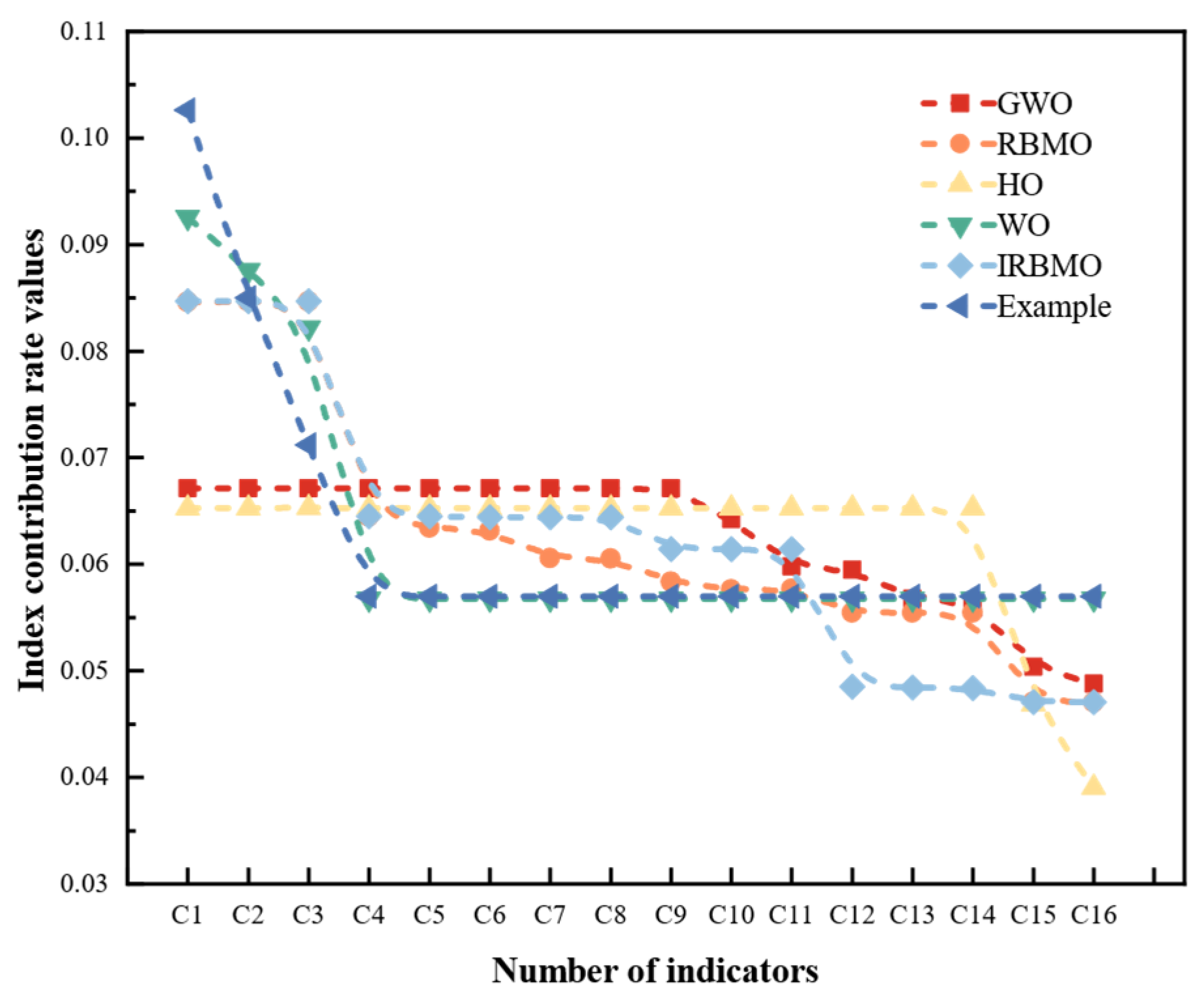
As illustrated in Figure 3, the results derived in Reference [53], without employing optimization algorithms, are relatively simplistic, whereas those obtained via most optimization algorithms are comparatively more complex. This complexity better reflects the disparities among indices and aligns more closely with practical scenarios. As presented in Table 10, the results are achieved by minimizing the fitness function value. The fitness function value for the case in Reference [53], calculated via Equation (4), is 2.1433, whereas the values obtained via optimization algorithms are consistently lower. Notably, the RBMO algorithm demonstrates exceptional performance. Upon further optimization based on RBMO, the IRBMO algorithm yields an even smaller fitness function value, driving the result closer to the ideal solution.

3.2.3. Stability and Efficiency Analysis of the IRBMO-G1 Algorithm

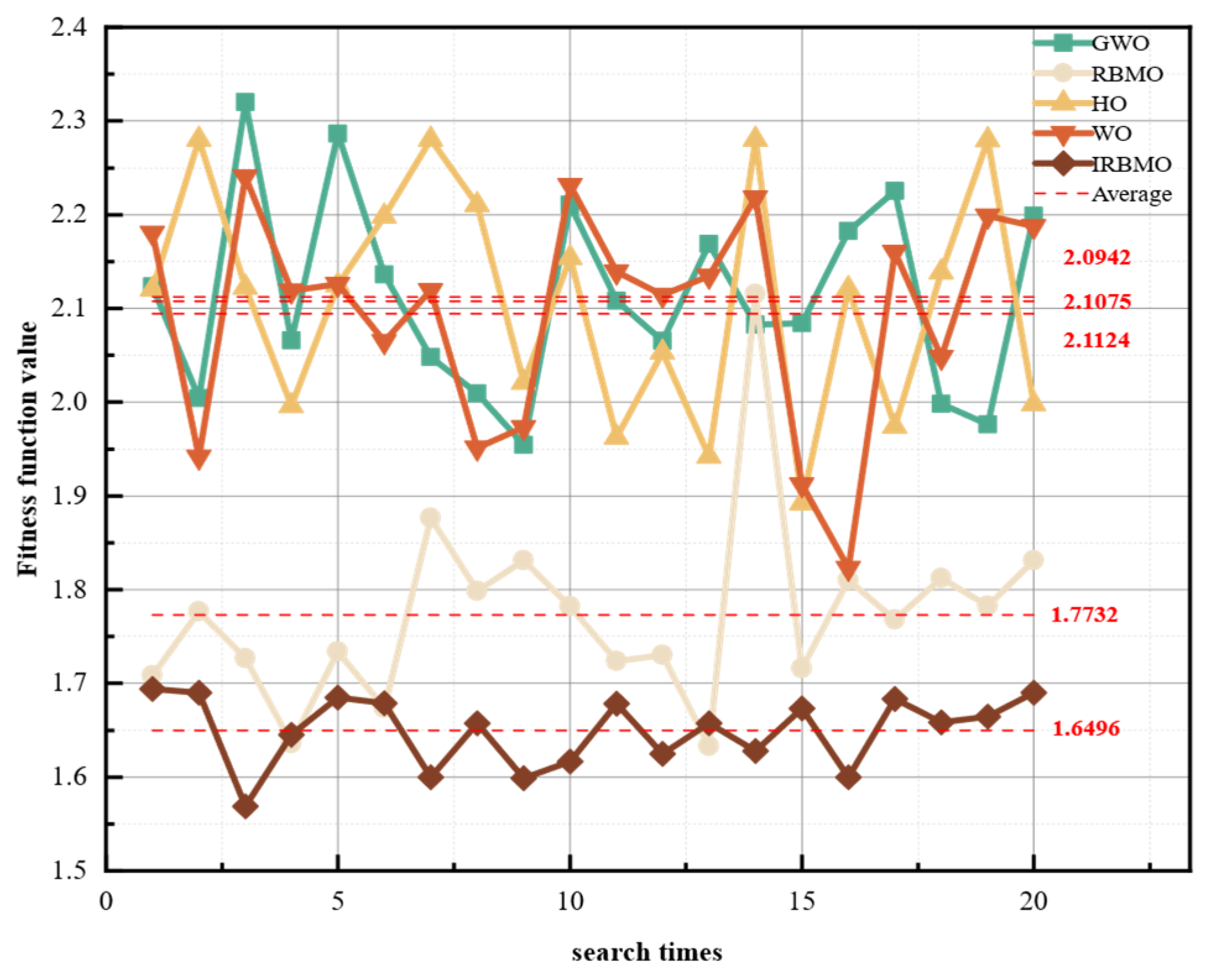
To comprehensively assess the stability and efficiency of the IRBMO-G1 algorithm in determining evaluation index contribution rates, this study utilizes the numerical example in Reference [53] as the test foundation. Three optimization algorithms, alongside the proposed RBMO and IRBMO algorithms, are employed to conduct 20 independent repeated trials on this case, enabling a comparative analysis focusing on search stability and convergence speed. The statistical results of the fitness function values acquired by each algorithm over the 20 runs are presented in Table 11, and the comparative curves of the fitness function search results are illustrated in Figure 4.
Figure 4 illustrates the distribution of fitness function values across 20 independent runs for various algorithms. As intuitively observed from the figure, the results of the IRBMO algorithm are confined to a narrow interval between 1.5689 and 1.6941, with a maximum fluctuation amplitude of merely 0.1252, substantially smaller than those of the comparative algorithms. This outcome indicates that the IRBMO algorithm exhibits consistent high-quality solution capability across multiple independent computations, being minimally affected by the randomness of the initial population. As indicated in Table 11, the standard deviation of the IRBMO algorithm is merely 0.0364, significantly outperforming the other algorithms. A reduced standard deviation demonstrates superior algorithmic robustness and greater stability in the solution results. Compared with the original RBMO algorithm, the standard deviation of the IRBMO algorithm is reduced by 63.8%, sufficiently substantiating the effectiveness of the improvement strategies in enhancing algorithmic stability. Furthermore, the minimal disparity between the optimal value (1.5689) and the worst value (1.6941) of the IRBMO algorithm further corroborates its exceptional stability performance.
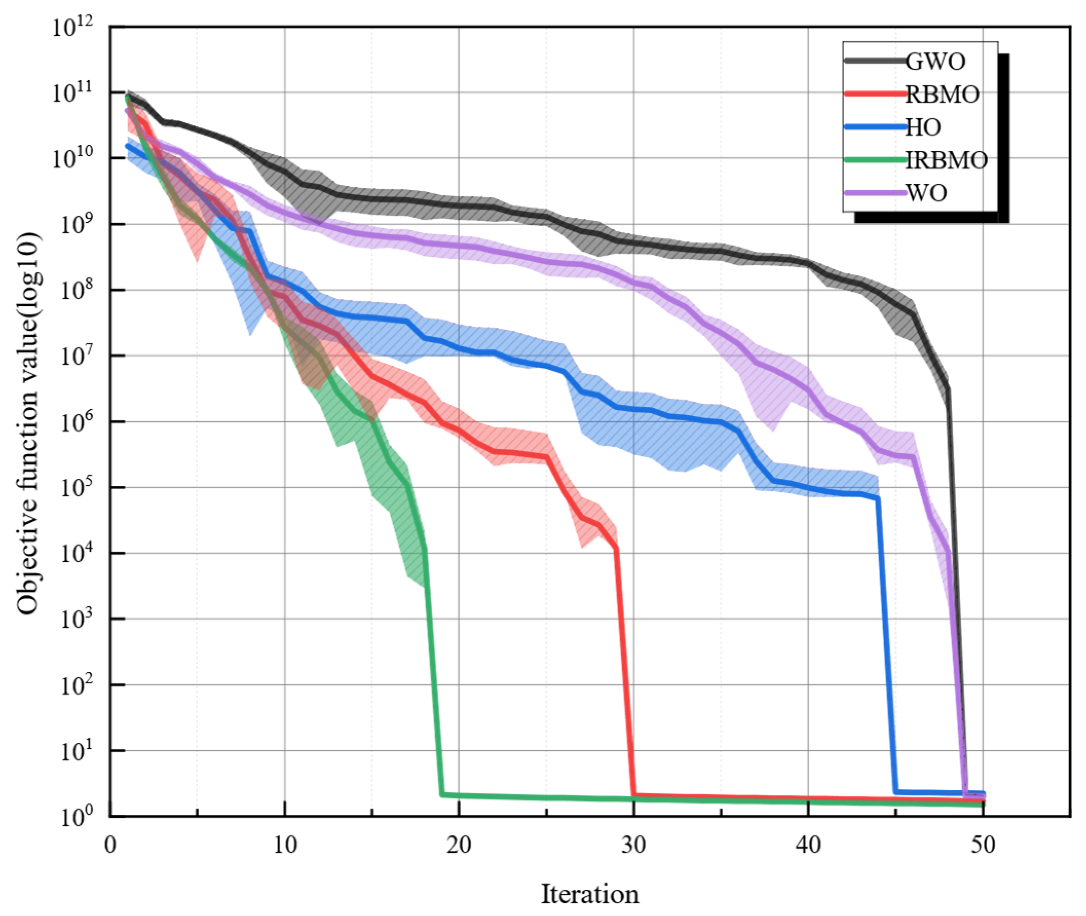
Figure 5 illustrates the average convergence curves and ±1 standard deviation ranges of the GWO, RBMO, HO, IRBMO, and WO algorithms across 20 runs. Due to the substantial variation span in the fitness function values among the algorithms, the vertical axis is represented using a logarithmic scale. As observed from the figure, IRBMO exhibits a rapid fitness decline rate during the early iterative phase and converges to a lower fitness level at approximately the 19th iteration, substantially earlier than RBMO, HO, WO, and GWO. Furthermore, the narrow standard deviation shadow region around the IRBMO curve indicates minimal fluctuation across multiple runs, demonstrating superior convergence stability. Overall, IRBMO demonstrates commendable comprehensive performance in terms of convergence speed, final fitness value, and operational stability.

3.2.4. Statistical Significance Test of Algorithm Performance

Given that all optimization algorithms exhibit random initialization and stochastic search characteristics, merely comparing the optimal values, mean values, or standard deviations across 20 independent runs is insufficient to ascertain whether the performance differences are statistically significant. Consequently, this study further employs the nonparametric Mann–Whitney U test to conduct a significance analysis on the fitness function values of different algorithms. Utilizing IRBMO as the baseline, pairwise comparisons are performed between its 20 fitness function values and those of GWO, HO, WO, and RBMO, respectively, with the significance level established at 0.05. When p < 0.05, the distributions of fitness function values between the two algorithms are considered to exhibit a significant difference. The specific results are presented in Table 12.
The Mann–Whitney U test results indicate that the p-values between IRBMO and each comparative algorithm are consistently below 0.05, demonstrating that the fitness function values obtained by IRBMO across 20 independent runs exhibit statistically significant differences from those of the other algorithms. Synthesizing the preceding results regarding mean values, standard deviations, and convergence curves, it can be concluded that IRBMO possesses superior solution stability and optimization performance in the contribution rate optimization problem.

3.3. Determination of Objective Weights via the Entropy Weight Method

To enhance evaluation objectivity, the Entropy Weight Method (EWM) is introduced to calculate the objective weights. Entropy, a concept originating from thermodynamics [54], denotes the degree of chaos or disorder within a system. It is incorporated into the evaluation system as a metric for the dispersion degree of indices. The procedures for calculating weights using the EWM are as follows:
(1)
Construction of the original matrix X and data standardization.
The original matrix X = (xij)m×n is constructed. Equation (2) is utilized to eliminate the dimensional effects among indices and unify their directions, with the standardized values denoted as zij.
(2)
Calculation of the entropy value Ej for each index.
E j = 1 ln m i = 1 m P i j ln P i j
P i j = z i j i = 1 m z i j
where j = 1, 2, …, n, with PijlnPij defined as 0 when Pij = 0.
(3)
Calculation of the objective weight of the j-th index.
w j = 1 E j j = 1 n ( 1 E j )
Based on the aforementioned equation, the objective weight vector wobj = (w1, w2, …, wn) is obtained.

3.4. Combined Weighting Method Based on Game Theory

In multi-attribute decision-making, subjective weights reflect decision-makers’ experience, whereas objective weights rely on the intrinsic data; however, employing a singular weighting scheme often introduces deviations. Guided by the Nash equilibrium concept, the subjective and objective weights are optimized based on game theory to achieve an optimal balance during this “game”, thereby preserving subjective judgments while conforming to underlying data patterns [55]. With the objective of deviation minimization [56], the obtained subjective and objective weights are integrated for combined weighting calculation utilizing optimal weight allocation coefficients. The deviation minimization objective is defined as minimizing the sum of squared Euclidean distances between the combined weight and each fundamental weight, whereby the objective function is formulated as follows:
J = min i = 1 n ( w i w s i ) 2 + ( w i w o i ) 2
Compared with simple weighted averaging, multiplicative combination, the general distance method, or set weighting methods, game-theoretic combined weighting eliminates the need to artificially preset the proportion of subjective and objective weights. It precludes excessive compression of an indicator’s role due to an excessively marginal single weight and provides a more transparent decision-making rationale. Furthermore, it automatically adjusts the combination coefficients according to the variations among different weight vectors, ultimately generating a combined weight that embodies an equilibrium compromise between the two. The deviation minimization objective value quantifies the overall deviation between the combined weight and the respective weights, with a lower value signifying superior consistency. According to the properties of matrix differentiation, Equation (20) is transformed into the system of linear equations depicted in Equation (21), thereby ultimately yielding the optimal weight allocation coefficients.
w o w o T w o w s T w s w o T w s w s T α o α s = w o w o T w s w s T
w = α o α o + α s w o + α s α o + α s w s
where ws denotes the subjective weight vector, wo represents the objective weight vector, αs is the subjective weight allocation coefficient, and αo is the objective weight allocation coefficient.

4. Fuzzy Comprehensive Evaluation of the Geological Environment in Abandoned Open-Pit Mines

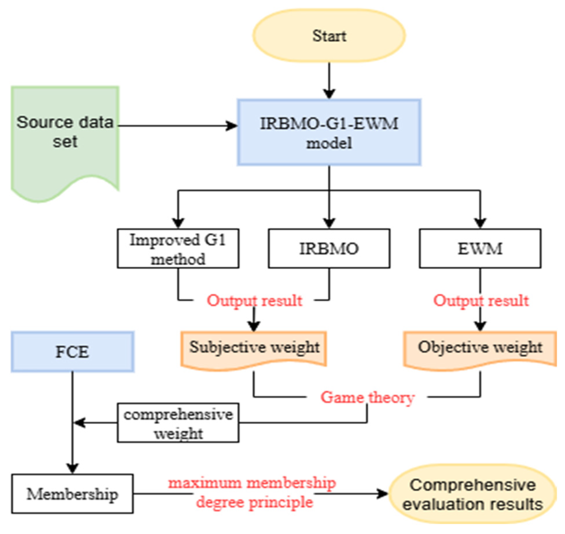
This study employs the IRBMO-G1-EWM-FCE three-level fusion framework to accomplish a multi-dimensional quantitative assessment of the geological environment in abandoned open-pit mines. The subjective weights of the indices are determined via the improved G1 method integrated with the IRBMO algorithm; the data-driven objective weights are acquired through EWM analysis; and based on the game-theoretic combination optimization theory, the subjective and objective weights are fused to derive the combined weights of the 13 indices. On this basis, the fuzzy comprehensive evaluation method is applied to conduct grade classification for the geological environment of abandoned open-pit mines according to the principle of maximum membership degree. The specific flowchart of the evaluation process is illustrated in Figure 6.

4.1. Fuzzy Comprehensive Evaluation Method

The Fuzzy Comprehensive Evaluation (FCE) method is an evaluation approach integrating qualitative and quantitative analyses [57]. Grounded in fuzzy mathematics, it conducts a comprehensive assessment of the membership grade status of evaluated subjects across multiple factors. The specific procedures are as follows:
(1)
Establishment of the evaluation factor set.
The evaluation factor set represents the aggregation of various evaluation indices, denoted as U, namely U = {U1, U2, …, Un}, where n signifies the number of indices. The factor set defined in this study is U = {rock type U1, hydrogeological conditions U2, topography and geomorphology U3, seismic intensity U4, geological structures U5, land destruction area U6, exposed rock wall ratio U7, aquifer destruction degree U8, landscape destruction ratio U9, comprehensive soil and water pollution degree U10, geological disaster scale U11, geological disaster quantity U12, soil erosion U13}, with n = 13.
(2)
Establishment of the evaluation grade set.
The evaluation grade set comprises all potential evaluation grades that evaluators may assign to the evaluated subjects. Based on practical evaluation requirements, the evaluation grade set is established and denoted as V = {V1, V2, …, Vm}, where m represents the number of evaluation grades. This study categorizes the evaluation grades into three levels, namely V = {Grade I (favorable), Grade II (poor), Grade III (severe)}.
(3)
Determination of the index weight set.
Weights are metrics quantifying the degree of influence of individual evaluation indices on the final results, denoted as W = {w1, w2, …, wn}. Weights are classified into subjective and objective categories. This study employs the IRBMO-G1-EWM to calculate the subjective and objective weights, and subsequently integrates them via game theory to derive the combined weight w.
(4)
Construction of the membership function.
The membership function signifies the degree to which an evaluation index belongs to a specific evaluation grade. Numerous methods exist for determining membership functions, encompassing rectangular and trapezoidal distribution functions. In geological environment evaluations, the trapezoidal distribution function is predominantly adopted as the membership function [32,58], as expressed in the following equation:
D 1 = 1 ,   x x 1 x 2 x x 2 x 1 ,   x 1 < x < x 2 0 ,   x x 2   , D 2 = x x 1 x 2 x 1 ,   x 1 < x < x 2 1 ,   x 2 x x 3 x 4 x x 4 x 3 ,   x 3 < x < x 4 0 ,   x x 4   o r   x x 1   , D 3 = 0 ,   x x 3 x x 3 x 4 x 3 ,   x 3 < x < x 4 1 ,   x x 4  
where D1, D2, and D3 denote the membership degrees of the three evaluation grades, whereas x1, x3, and x5 represent the standard values for these grades. Additionally, x2 and x4 signify the upper limits of the concentrated transition intervals. The methods for determining their values are as follows:
x 2 = x 1 + β ( x 3 x 1 ) x 4 = x 3 + β ( x 5 x 3 )
where β denotes the interval transition coefficient, which is set to 0.5 in this study.
(5)
Establishment of the factor fuzzy matrix.
As each evaluation index is assessed against the evaluation grade set, let Rnm denote the membership degree of the nth element in the factor set with respect to the mth grade in the evaluation grade set. Consequently, the fuzzy matrix for an index can be constructed as follows:
R n × m = R 11 R 1 m R n 1 R n m
(6)
Comprehensive evaluation.
The final comprehensive evaluation results are derived by performing operations on the weight set and the factor fuzzy matrix. The specific computational procedure is expressed as follows:
T = W T × R n × m = w 1 , w 2 w n × R 11 R 1 m R n 1 R n m
where WT denotes the weight set of the evaluation indices, and T represents the comprehensive evaluation result.
According to the principle of maximum membership degree, the evaluation grade corresponding to the highest membership degree within the comprehensive evaluation result is designated as the geological environment evaluation grade of the abandoned open-pit mine.

4.2. Case Study

4.2.1. Overview of the Study Area

(1)
Regional and Geological Background
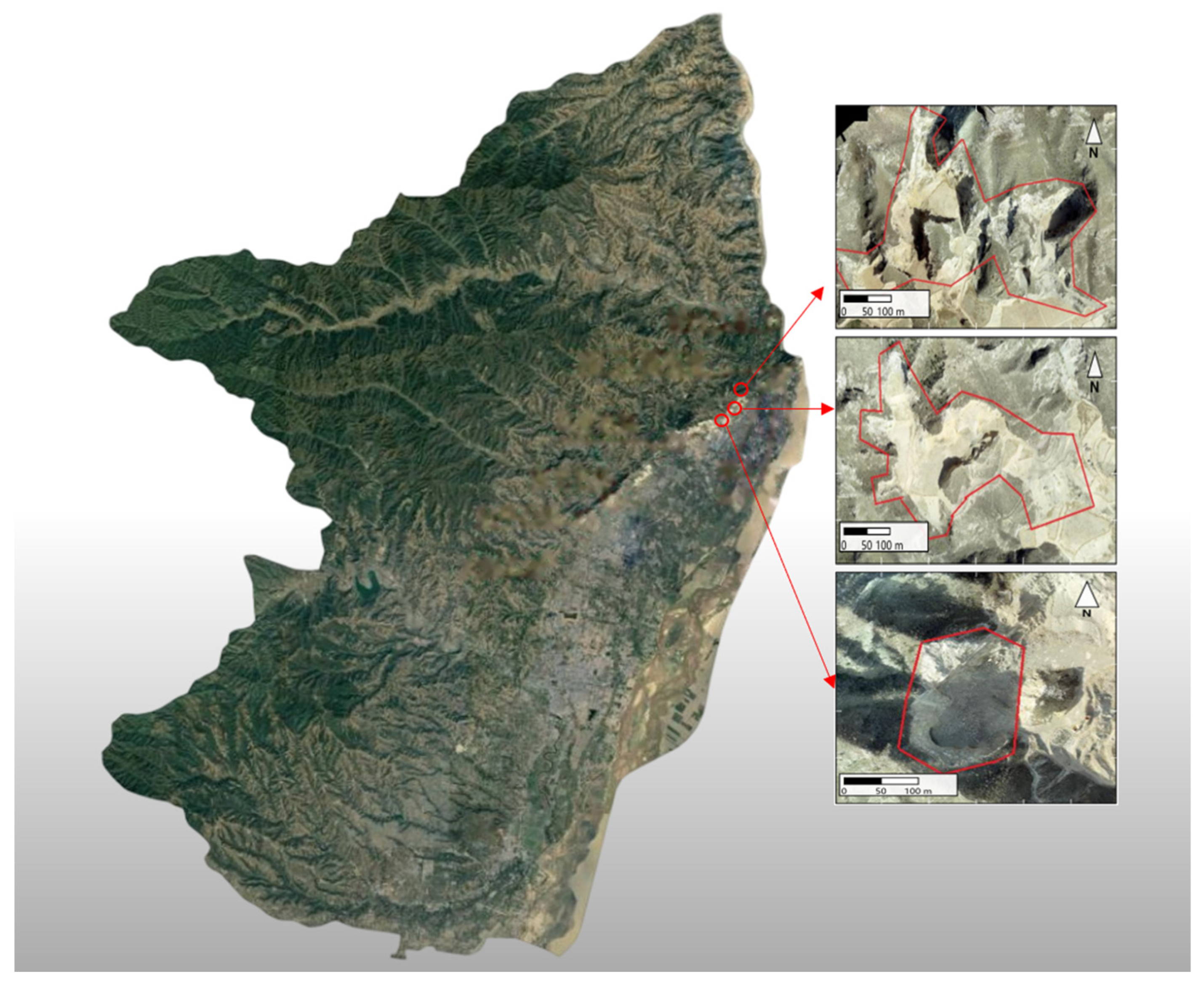
This study selects the Zhubei 1# Quarry, Zhubei 2# Quarry, and Zhubei 3# Quarry, located within the territorial spatial ecological restoration demonstration project area for ecological protection and high-quality development in the Yellow River Basin, to conduct the geological environment evaluation of abandoned open-pit mines. Hereafter, Quarry A, Quarry B, and Quarry C are utilized to represent the three aforementioned quarries, respectively. The study area is situated in Shaanxi Province, China, at longitudes 110°34′20″ to 110°35′10″ E and latitudes 35°38′41″ to 35°38′56″ N. The geomorphology is predominantly characterized by low mountains and hills, with the terrain being higher in the northwest and lower in the southeast. Its planar morphology exhibits an elongated configuration with alternating steep and gentle sections, wherein bedrock is extensively exposed along the steep wall segments. No conspicuous geological structures such as folds and faults exist within the region; however, the joints and fissures within the rock mass are extremely developed, resulting in a highly fragmented rock mass. The excavation periods of the three mining pits were predominantly concentrated in the 1980s and 1990s, and they were closed around 2010. Prolonged bottom blasting excavation has generated high and steep rocky slopes, exposed rock walls, residual hills at the pit bottoms, and concave basin-shaped mining pits. The lithology is primarily composed of dark gray medium-thick bedded fine-crystalline limestone, brecciated limestone, and dolomite, intercalated with thin-bedded argillaceous limestone and dolomitic limestone. Owing to the spatial concentration of the three quarries, Figure 7 adopts an approach combining the research area scale and the quarry scale to illustrate the location of the project area, the spatial relationships among the three quarries, and their local topographical and geomorphological characteristics. The peak ground acceleration in this area is 0.15 g, corresponding to a basic seismic intensity of VII, with a characteristic period of the seismic response spectrum of 0.40 s.
(2)
Comparative Geological and Rock-mass Characteristics of the Three Quarries
To further elucidate the geological similarities and differences among the three quarries, this study compiles data on the exposed rock wall scale, rock mass fragmentation characteristics, rock mass quality grades, and geological hazards of Quarries A, B, and C based on mining area exploration data and research reports. The results are presented in Table 13. This information is primarily utilized to delineate the engineering geological background of the three cases and provide a basis for the subsequent assignment of evaluation index values.
As indicated in Table 13, the three quarries exhibit strong similarities in regional location, mining history, predominant lithology, and hydrogeological conditions, whereas prominent differences exist among them regarding mining pit morphology, scale of exposed rock faces, land damage area, and developmental degree of geological hazards. Quarry A exhibits a substantial land damage area and a large number of developed collapses. Quarry B displays pronounced high, steep slopes and pit floor disturbance, and Quarry C features a comparatively minor land damage area and a number of identified collapses. These discrepancies furnish an engineering geological basis for the subsequent assignment of values for indices, including land damage area, proportion of exposed rock faces, magnitude of geological hazards, and number of geological hazards.
(3)
Data Processing
To facilitate subsequent weight calculations, qualitative indices were quantified. Based on the aforementioned evaluation criteria, three levels (minor, relatively severe, and severe) were set to 1, 2, and 3, respectively. The quantitative values of the evaluation indices for each quarry are presented in Table 14.

4.2.2. Calculation of Index Weights

  • Calculation of subjective and objective weights via IRBMO-G1-EWM
To mitigate individual expert bias, five experts from disciplines including mine geological environment investigation, geotechnical engineering, geological hazard prevention and control, and ecological restoration were invited to participate in the index ranking. Initially, each expert independently ranked the 13 evaluation indices by importance and assessed the relative importance of adjacent indices. Following aggregation of the expert ranking results and confirmation via a consistency test that the ranking outcomes possessed acceptable consistency, a new sequence was obtained: U11 > U12 > U5 > U2 > U6 > U8 > U13 > U7 > U10 > U9 > U4 > U1 > U3. The importance degrees of the ranked indices were subsequently compared to derive rk = {1.2, 1.2, 1.4, 1.4, 1.6, 1.2, 1.2, 1.0, 1.0, 1.2, 1.0, 1.2}, followed by data standardization, as presented in Table 15.
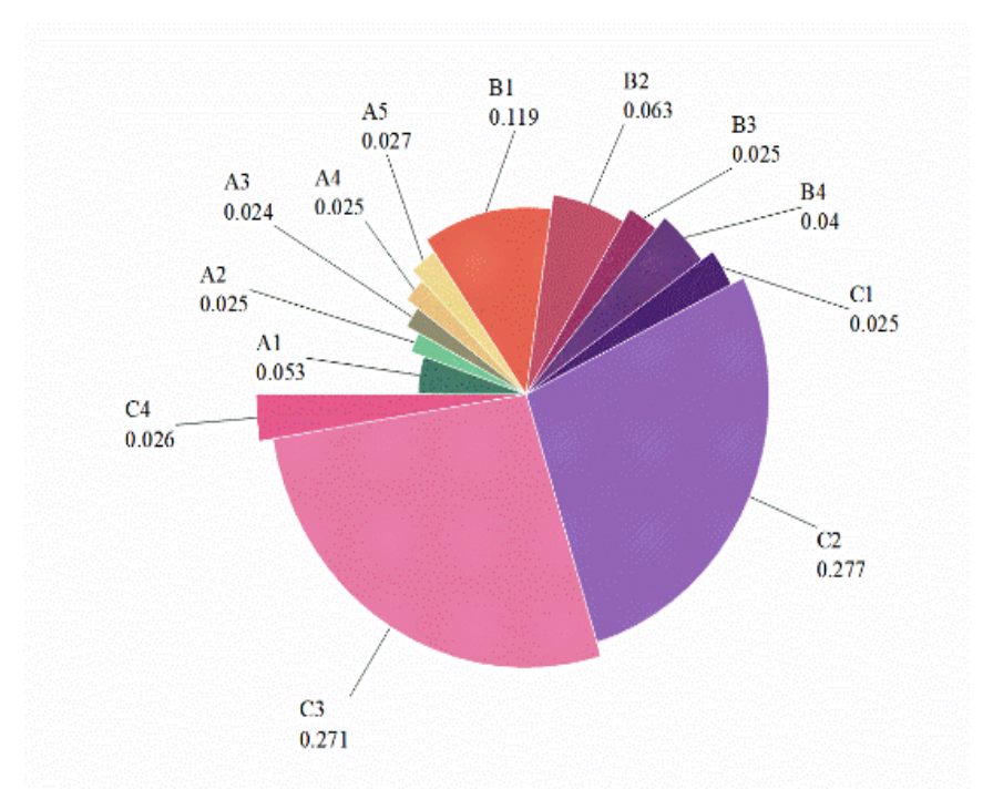
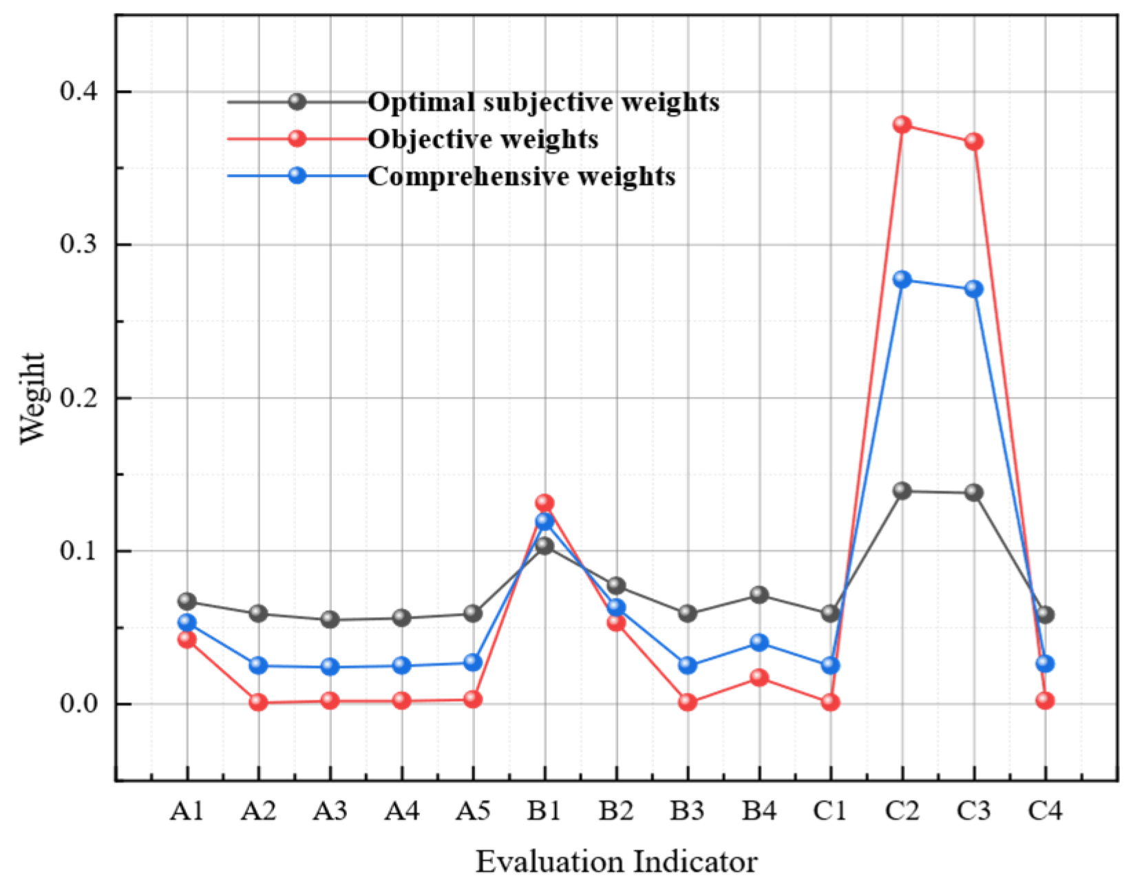
By applying the IRBMO-G1 algorithm to calculate the optimal index contribution rates, the values for each index were determined to be 0.0836, 0.0807, 0.0776, 0.0776, 0.0772, 0.0769, 0.0768, 0.0768, 0.0768, 0.0768, 0.0735, 0.0735, and 0.0722, respectively. Based on Equation (5), the optimal subjective weights for indices U1 through U13 were derived as 0.067, 0.059, 0.055, 0.056, 0.059, 0.103, 0.077, 0.059, 0.071, 0.059, 0.139, 0.138, and 0.058, respectively. Utilizing the standardized data presented in Table 15, the objective weights for each index were calculated via Equations (17)–(19) as 0.042, 0.001, 0.002, 0.002, 0.003, 0.131, 0.053, 0.001, 0.017, 0.001, 0.378, 0.367, and 0.002.
b.
Determination of Combined Weights
Based on game theory, the subjective and objective weights were integrated. According to Equation (21), the weight allocation coefficients were determined as αs = 0.4732 and αo = 0.6523, which, after normalization, yielded 0.4204 and 0.5796, respectively. Through the combinational allocation of the subjective and objective weights, the final combined weights were obtained, as illustrated in Figure 8.
Figure 9 illustrates the comparison curves of the subjective, objective, and combined weights, demonstrating that single weighting methods exhibit significant limitations when processing evaluation indices. Subjective weights lean towards global trade-offs with minor fluctuations, ensuring comprehensive coverage across evaluation dimensions. Conversely, objective weights are constrained by the discrete characteristics of the original data, demonstrating a concentration of weights among a minority of indices. In contrast, the combined weights, integrated via game theory, not only retain the sensitive capture of highly distinguishable indices by objective data but also leverage expert experience to correct the risk of index marginalization inherent in objective weighting, thereby significantly enhancing the robustness of the evaluation system.

4.2.3. Comprehensive Evaluation of the Geological Environment in Abandoned Open-Pit Mines

Building upon the combined weights, the FCE was employed to evaluate three quarries within the study area. By calculating the membership degrees of the evaluation indices across different evaluation levels according to Equation (23) and utilizing them as the fuzzy evaluation sets, the fuzzy relation matrices for the three quarries were derived as follows:
R a = 1 1 0 0 0 0 0 1 0 1 1 0 0 0 0 1 0 0 1 0 0 0 0 0 0 0 0 0 0 1 1 0 1 0 1 0 0 1 1 T
R b = 1 1 0 0 0 0 0 1 0 1 1 0 0 0 0 1 0 0 1 0.565 0 0 0 0 1 0 0 0 0 1 1 0 0.435 0 1 0 0 0 1 T
R c = 0 1 0 0 0 1 0 1 0 1 1 1 0 1 0 1 0 0 0 0 0 0 0 0 0 0 0 0 0 1 1 0 1 0 1 0 0 0 1 T
By integrating the weight set with the fuzzy factor matrix, the membership degree values for each grade were derived, and the final evaluation grades were determined based on the maximum membership degree principle, as presented in Table 16.
As indicated in the table, the evaluation results for the three quarries are Grade III for quarry a, Grade II for quarry b, and Grade I for quarry c. The geological environment conditions across the three quarries demonstrate notable divergence. Despite Quarry A exhibiting minor rock weathering and low pollution levels, it contains up to 11 collapses with a total volume of approximately 5950 m3, substantially exceeding those of the other two quarries. Furthermore, it possesses the largest land damage area, acting as the critical index that downgrades its evaluation grade to “Severe”. Quarry B is characterized by a high landscape destruction rate coupled with the occurrence of certain geological hazards. Although its overall ecological functions have been severely impaired, its risk level remains slightly lower than that of Quarry A. Quarry C represents a typical mining area that is small in scale and highly disturbed yet low in risk. Despite its relatively high landscape destruction rate, it exhibits minimal potential for geological hazards and retains a certain capacity for natural recovery. Consequently, relative to the other two quarries, its geological environment demonstrates greater stability.

4.2.4. Sensitivity and Robustness Analysis

To examine the sensitivity of the evaluation results to the uncertainty of key parameters, a sensitivity analysis is performed. The evaluation process involves parameters including expert ranking, adjacent importance ratio rk, subjective weights, game-theoretic combination coefficients, and membership transition coefficient β, wherein a variation in any single parameter may impact the final combined weights, comprehensive membership vector, and evaluation grade. This study employs the grade stability rate to characterize the stability of the evaluation grade against weight perturbations. The grade stability rate is defined as the ratio of the frequency with which the evaluation grade remains consistent with the original evaluation grade during perturbation simulations to the total number of simulations. The sensitivity analysis scheme is presented in Table 17.
Wherein, ε denotes a random perturbation term conforming to a uniform distribution. When the perturbed rk, αs, or β exceed their reasonable value ranges, truncation is applied according to the original parameter intervals to ensure the perturbation outcomes retain practical significance.
As indicated in Table 18, the impacts of various parameter perturbations on evaluation grade stability exhibit pronounced differences. Under perturbation magnitudes of ±5%, ±10%, and ±20% applied to the subjective weights, game-theoretic combination coefficients, and membership transition coefficient β, the grade stability rates of the three quarries consistently equal 100%. This demonstrates that the final evaluation grades remain unaltered under reasonable fluctuations of these parameters, indicating that the evaluation results possess favorable overall robustness. The evaluation results demonstrate greater sensitivity to the expert ranking and adjacent importance ratio rk. Under expert ranking perturbations, the grade stability rates for Quarries A, B, and C are 91.7%, 75%, and 100%, respectively, indicating that Quarry B is the most sensitive to variations in the expert ranking. The perturbation outcomes for rk manifest analogous patterns: under a perturbation amplitude of ±5%, the evaluation grades of all three quarries remain stable; as the amplitude escalates to ±10% and ±20%, the grade stability rate of Quarry B declines to 89.5% and 67%, respectively, with Quarry A likewise decreasing to 98% under the ±20% perturbation, whereas Quarry C consistently retains 100%. This signifies that the evaluation grade of Quarry C exhibits the utmost stability, whereas Quarry B is presumably positioned in proximity to the evaluation grade boundary, rendering its final grade more susceptible to variations in subjective ranking and rk values. Overall, with the exception of substantial rk perturbations and expert ranking variations, the proposed model sustains stable evaluation grades under the majority of parameter perturbation conditions, substantiating the fundamental reliability of the evaluation results; nevertheless, this concurrently underscores that expert ranking and rk assignment should be rigorously regulated as pivotal control elements during model application.
It is noteworthy that the sensitivity analysis concurrently demonstrates that the evaluation grade of Quarry B exhibits considerable sensitivity to perturbations in expert ranking and variations in the value of rk. Under perturbations of expert ranking, the grade stability rate of Quarry B is 75%; when the perturbation amplitude of rk increases to ±20%, its grade stability rate declines to 67%. This indicates that the Grade II evaluation result for Quarry B is not entirely robust but is significantly influenced by subjective ranking and the determination of adjacent importance ratios. In other words, Quarry B is likely situated near the grade boundary between Grade I and Grade II or between Grade II and Grade III; its final grade should be regarded as an outcome derived from the current expert judgments and parameter configurations, rather than interpreted as an absolutely deterministic classification. Consequently, in practical applications, when an evaluation object exhibits a low grade stability rate or a marginal difference between the maximum membership degree and the membership degree of the adjacent grade, model practitioners should not yield a singular grade conclusion solely based on the maximum membership principle; instead, it ought to be identified as a boundary evaluation object. For such objects, it is recommended to formulate a comprehensive judgment incorporating field verification, expert reevaluation, supplementary investigation of key indicators, and dynamic monitoring results, and to adopt a relatively conservative management strategy in governance decision-making.
The grade stability rate primarily reflects whether the final evaluation grade alters following parameter perturbation, yet it cannot directly elucidate the inherent stability of the weight structure. Since the evaluation results in this study rely on the allocation of combined weights, a substantial shift in combined weights despite an unaltered evaluation grade following perturbation may still compromise the interpretability of the evaluation outcomes. Consequently, building upon the grade stability rate analysis, this study further computed the mean combined weights for each indicator following subjective weight perturbation and compared them with the original combined weights to examine the stability of the weight allocation structure under perturbation conditions. The results are presented in Table 19.
As indicated in Table 19, following perturbations of ±5%, ±10%, and ±20% applied to the subjective weights, the mean combined weights of each index generally remain proximate to the original combined weights, exhibiting no significant deviation. Indices with higher weights consistently maintain elevated weight levels across various perturbation amplitudes, whereas indices with lower weights demonstrate no anomalous amplification induced by the perturbations. This demonstrates that although subjective weight perturbations induce minor fluctuations in individual computational outcomes, the combined weight structure remains globally stable from the perspective of the averaged results across 200 perturbations. In conjunction with the grade stability rate results in Table 18, the proposed model sustains relatively stable weight allocations and evaluation grades under conditions of inherent uncertainty in subjective weights, thereby indicating that the evaluation results possess favorable robustness.
To further investigate whether the assignment method for qualitative indices influences the final evaluation grade, this study conducted a supplementary sensitivity analysis on the encoding scheme for qualitative indices. During the original evaluation process, qualitative indices including A1, A2, A3, A5, B3, and C4 utilized a 1/2/3 scale to respectively denote three severity grades: slight, moderately severe, and severe. Considering that this assignment method implicitly assumes equidistance between adjacent grades, this study further adopted a 1/3/5 scale as an alternative encoding scheme, while preserving the original values of quantitative indices, including A4, B1, B2, B4, C1, C2, and C3. Under the alternative encoding condition, data standardization, IRBMO-G1 subjective weighting, EWM objective weighting, game theory combined weighting, and FCE comprehensive evaluation were re-executed to examine whether the final grade is artificially induced by the encoding scheme of qualitative indices.
As observed in Table 20, when the encoding scheme for qualitative indices is adjusted from 1/2/3 to 1/3/5, although the membership degree vectors of the three quarries undergo certain variations, the final evaluation grades remain unchanged, with Quarries A, B, and C classified as Grade III, Grade II, and Grade I, respectively. This demonstrates that the final grades in this study are not artificially induced by the 1/2/3 encoding scheme, and the evaluation results exhibit a certain robustness to the encoding scheme for qualitative indices. Nevertheless, varying encoding schemes continue to influence the magnitudes of membership degrees and weight distributions; consequently, the uncertainty arising from the quantification of qualitative indices remains a limitation of the proposed method. Future research may employ interval numbers, fuzzy linguistic variables, or expert scoring distributions to further mitigate the impact of encoding assumptions.

4.2.5. Comparative Analysis of Different Evaluation Methods

To ascertain whether the proposed evaluation method yields divergent evaluation outcomes, this study compares it with two alternative methodologies: AHP-EWM-FCE and IRMO-FAHP-EWM-FCE. The three methodologies employ identical evaluation indices, grade criteria, measured index values, and fuzzy comprehensive evaluation procedures, with discrepancies residing exclusively in the weight determination methods. Consequently, the comparative outcomes can reflect the impacts of disparate weighting mechanisms on the final evaluation grade and membership degree vector. The final evaluation results of the three methodologies are presented in Table 21.
As indicated in Table 21, the final evaluation grades for the three quarries remain consistent across the three methods: Grade III for Quarry A, Grade II for Quarry B, and Grade I for Quarry C. This demonstrates that under an identical index system and FCE framework, the three combined weighting methods exhibit favorable consistency in overall grade determination. Nevertheless, the membership degree values reveal that disparate weighting methods still influence the membership distribution of each quarry across different grades. To further quantify discrepancies among different evaluation methods regarding the final membership degree distribution, the proposed method is utilized as the benchmark, and two indices, Euclidean distance and maximum membership degree difference, are introduced for comparison. The Euclidean distance serves to measure the overall discrepancy between the membership degree vectors derived from the two methods, with its calculation formula expressed as
d E = k = 1 3 D k 1 D k 2 2
where Dk1 denotes the membership degree value of the kth evaluation grade derived from the proposed evaluation method, and Dk2 denotes the membership degree value of the kth evaluation grade derived from the comparative evaluation method.
As the evaluation grades in this study comprise Grades I, II, and III, the evaluation outcome of each evaluated object can be represented as a three-dimensional membership degree vector. A diminished Euclidean distance signifies closer proximity between the membership degree distributions derived from the two methods. Simultaneously, to identify the maximum deviation at a singular evaluation grade, this study further calculates the membership degree value differences between each comparative method and the proposed method. The evaluation grade exhibiting the maximum membership degree value difference reflects the most substantial divergence between the two methods at that specific grade. Compared with the Euclidean distance, this metric facilitates a more straightforward determination of which evaluation grade the discrepancies predominantly concentrate upon. Given that the final evaluation grade is determined by the maximum membership degree principle, the maximum membership degree difference can assist in adjudicating whether disparate weighting methods might alter the grade determination outcomes.
Table 21 and Table 22 demonstrate that the three methods yield identical final evaluation grades for the three quarries, with marginal variations in membership degree vectors and Euclidean distances ranging from 0.014 to 0.073. This indicates that under the identical index system, classification standards, and FCE procedure, the final grades in this case exhibit a certain robustness to varying weighting mechanisms. Consequently, the practical contribution of the proposed method should not be interpreted as significantly altering the final evaluation grades; rather, it should be recognized as providing a more interpretable generation mechanism for subjective weights while preserving the stability of the evaluation grades. Compared with the AHP or FAHP methods, the IRBMO-G1 method obviates the necessity of constructing a complete pairwise comparison matrix; instead, it articulates subjective judgments through expert ranking and adjacent importance ratios, and utilizes IRBMO to optimize index contribution rates under weak consistency constraints. This renders the weight-formation process more transparent and parameter implications more explicit, and also facilitates subsequent sensitivity analyses and verifications.

4.3. Engineering Application Significance and Mine Restoration Management Implications

The ultimate objective of geological environment evaluation for abandoned open-pit mines extends beyond acquiring evaluation grades to providing a decision-making basis for mine ecological restoration and geological disaster prevention and mitigation. Consequently, it is imperative to further transform the model evaluation outcomes into remediation priorities and engineering management recommendations. Based on evaluation outcomes derived from the IRBMO-G1-EWM-FCE model, this study analyzes the engineering application significance from three aspects: remediation urgency, principal risk sources, and restoration measure selection. The engineering management implications of the evaluation results for the three quarries are shown in Table 23.
From a practical application perspective, the constructed IRBMO-G1-EWM-FCE model not only determines the geological environment quality grades of abandoned open-pit mines but also identifies the relative degradation degrees and remediation priorities among different quarries. For local natural resource administration departments and mine ecological restoration projects, this model facilitates rapid grading during preliminary investigation phases, differentiated allocation of remediation funds, and targeted selection of restoration measures. Compared to solely relying on empirical judgments, this method integrates expert knowledge, index data dispersion, and fuzzy grade classification, thereby rendering the evaluation results more interpretable and enhancing managerial operability. Particularly when multiple abandoned quarries require simultaneous remediation under limited financial and construction constraints, the model assists administrators in preferentially identifying quarries with elevated risks and pronounced remediation urgency, consequently augmenting the scientific rigor of mine ecological restoration decision-making.

5. Discussion

This study constructed a geological environment evaluation model for abandoned open-pit mines based on IRBMO-G1-EWM-FCE, applying it to three abandoned quarries within the ecological restoration demonstration project area of the Yellow River Basin in Shaanxi Province. The evaluation results demonstrate that this model comprehensively integrates expert judgment, index data dispersion, and fuzzy grade classification, providing a quantitative basis for geological environment grading and remediation priority identification of abandoned quarries. Nevertheless, the proposed method remains subject to the influences of factors including sample size, index weighting, grading thresholds, and the completeness of geomechanical data; consequently, it is imperative to further discuss the practical implications, methodological discrepancies, and limitations of the evaluation results.
(1)
In this study, objective weights occupy a relatively higher proportion, an outcome attributed to the sample data structure. The three quarries exhibit identical or marginally disparate values across certain indices, while demonstrating more pronounced discrepancies regarding indicators such as land damage area, geological hazard scale, and geological hazard quantity. EWM assigns greater weights to indices with higher dispersion. Consequently, objective weights concentrate predominantly on indices capable of differentiating quarry discrepancies. Within game theoretic combination weighting, combined weights are determined by minimizing deviations from both subjective and objective weights. When the objective weight vector incorporates more robust data-differentiation information, objective weights are liable to occupy a relatively higher proportion. Nevertheless, this does not imply that expert knowledge is attenuated to negligibility within the evaluation; expert rankings still participate in the combination weighting via subjective weights, thereby providing supplementation for indices characterized by low dispersion yet geological significance. It should be noted that, given merely three evaluation objects, the responsiveness of EWM to data dispersion might amplify the influence of individual indices. Consequently, the proportion of objective weights in this study should not be construed as objective weights being inherently superior to expert judgments under general circumstances.
(2)
Insufficient geomechanical information constitutes a significant limitation in the present case study. Although this study supplemented engineering geological information within the study area, including lithology, geomorphological configurations, joint and fissure development, and rock mass fragmentation degrees, the existing data remain insufficient for conducting rigorous rock mass quality classifications or slope stability analyses. Established rock mass classification methodologies, such as the RMR and Laubscher classification systems, typically necessitate parameters including rock uniaxial compressive strength, RQD, joint spacing, joint surface conditions, groundwater conditions, and the relationship between structural planes and slopes. However, the data available in this study cannot fully satisfy these computational requirements. Consequently, the proposed model is currently more applicable to the comprehensive evaluation of geological environment quality in abandoned open pit mines, and cannot substitute for specialized rock mass classifications or rock slope stability evaluations. Subsequent research incorporating systematic rock mass structural plane investigations, rock mechanics experiments, and rock mass classification outcomes such as RMR will facilitate further extending the application depth of this model in geological environment quality evaluations and slope stability assessments.
(3)
The proposed method is further constrained by expert judgment and small sample sizes. The IRBMO-G1 subjective weighting process relies on expert judgments regarding index importance rankings and adjacent importance ratios; different expert panels may yield disparate rankings, thereby influencing the subjective weights. Although sensitivity analysis can verify the stability of the final grades within a specific perturbation range, it cannot completely eliminate the uncertainty arising from discrepancies in expert consensus. Subsequent research should incorporate a larger pool of experts and integrate methodologies such as the Delphi method and the Kendall coefficient of concordance to enhance the consistency and reproducibility of expert rankings. Simultaneously, this study selected merely three abandoned quarries within the ecological restoration demonstration project area of the Yellow River Basin in Shaanxi Province, without expanding to a larger number of quarries or encompassing diverse geological regions, rock types, and climate zones. The objective weights derived via EWM should not be construed as stable statistical weights applicable to all abandoned open pit mines; rather, they should be regarded as modification terms based on data discrepancies for the expert subjective weights within the current case. The primary cause of this limitation lies in the substantial disparities frequently existing among geological survey data, engineering mapping accuracy, geological hazard records, ecological destruction indices, and restoration engineering data of abandoned quarries across different regions. Consequently, acquiring comparable data satisfying the requirements of an identical index system, identical grading standards, and identical survey scales remains challenging in the short term. Therefore, the evaluation results herein are more appropriate for methodological validation within engineering evaluation scenarios involving small samples, rather than being interpreted as predictive outcomes possessing broad regional representativeness. Beyond sample scale and the weight stability of EWM, the determination uncertainty of samples adjacent to grade boundaries constitutes another noteworthy issue in the application of the proposed model. The sensitivity analysis further reveals that the grade stability varies among different evaluation objects. Quarries A and C maintain high stability under the majority of perturbation conditions, whereas Quarry B exhibits pronounced sensitivity to perturbations in expert ranking and substantial amplitude perturbations in rk. This indicates that for evaluation objects approaching grade boundaries, the output grades of the model might be influenced by subjective judgment parameters. This finding constitutes a significant limitation in the application of the proposed method: although the IRBMO-G1-EWM-FCE model can provide quantitative grade classification, for boundary samples, their evaluation grades are more appropriate as references for risk identification and management zoning, rather than being regarded as absolutely deterministic discrimination results. In practical applications, the grade stability rate, membership degree distribution, and field conditions of key indices should be concurrently reported to enhance the transparency of evaluation conclusions and the reliability of decision-making.
(4)
Index grading thresholds, qualitative index quantification, and membership function configurations also influence the evaluation results. Several qualitative indices in this study are quantified utilizing 1, 2, and 3; although facilitating model computation, this processing approach inevitably simplifies complex geological environment conditions. For instance, indices including rock mass fragmentation degree, aquifer impact degree, and geomorphological type inherently possess continuity and fuzziness; representing them with singular integer values may obscure their internal discrepancies. Furthermore, the origins and configurations of classification thresholds impact index membership degrees. Particularly when specific index values approximate grade boundaries, marginal variations in thresholds or membership function conversion coefficients may alter the membership degree distributions. Although sensitivity analysis can ascertain whether evaluation grades maintain stability within a defined perturbation range, it cannot entirely substitute for further verification regarding threshold rationality and qualitative quantification uncertainties. Subsequent research may consider employing interval numbers, fuzzy linguistic variables, or expert scoring distributions to articulate the uncertainties inherent in qualitative indices, alongside integrating more substantial samples to examine the stability of grading thresholds, EWM weights, and final evaluation grades.
(5)
In this study, the correspondence between the evaluation results and field conditions serves solely for internal consistency verification, rather than constituting an independent external validation of the accuracy of the evaluation grades. Given the current absence of official geological environment grade classifications, blind review results from third-party experts, long-term monitoring data, or comprehensive historical disaster records independent of the model input data for the three quarries, this study is unable to establish a genuinely independent external validation benchmark. Consequently, this study cannot assert that the grades derived from the model have been corroborated by external data, nor can the correspondence between the evaluation grades and field conditions be interpreted as a confirmation of grade accuracy. This correspondence merely indicates that, under the current index system and input data, and evaluation procedure, the model outputs possess internal logical consistency with the primary geological environment characteristics observed in the field. Future research remains imperative to incorporate official investigation outcomes, independent expert evaluations, long-term monitoring data, and disaster event records to perform external validation on the model grades.

6. Conclusions

Addressing the pronounced uncertainty inherent in subjective weighting and the inadequacy of singular weighting methodologies to accommodate expert experience and data discrepancies within the geological environment evaluation of abandoned open pit mines, this study constructed the IRBMO-G1-EWM-FCE comprehensive evaluation model. This model was subsequently applied to the evaluation of geological environmental quality at three abandoned quarries within the ecological restoration demonstration project area of the Yellow River Basin in Shaanxi Province. The results demonstrate that this model effectively integrates expert ranking information, objective data dispersion, and the fuzzy comprehensive evaluation process, thereby providing an operational evaluation framework for grading the geological environment and identifying remediation priorities in abandoned open pit mines. The principal conclusions are as follows:
(1)
This study proposed a subjective weight determination method based on IRBMO-G1. Built upon the improved G1 method, this approach articulates subjective judgments through index importance rankings and adjacent importance ratios provided by experts, and utilizes the IRBMO algorithm to optimize index contribution rates, thereby acquiring subjective weights that satisfy weak consistency constraints. Compared with conventional AHP or FAHP methodologies, the IRBMO-G1 method circumvents the construction of complete judgment matrices and the need for consistency adjustment procedures, exhibiting superior interpretability and operability.
(2)
The RBMO algorithm was improved utilizing Circle chaotic mapping and Cauchy mutation strategies, and the optimization performance of the IRBMO algorithm was validated through CEC2017 benchmark function tests, convergence curve analyses, and computational efficiency comparisons. The results demonstrate that IRBMO exhibits favorable search precision, convergence speed, and stability across the majority of test functions and the weight optimization problem addressed in this study.
(3)
Based on the results of IRBMO-G1, EWM, and game theoretic combination weighting, this study employed the FCE method to evaluate the geological environment quality of three abandoned quarries. The results indicate evaluation grades of Grade III, Grade II, and Grade I for Quarries A, B, and C, respectively, demonstrating variances in their geological environment degradation degrees and remediation urgency. Specifically, Quarry A is notably affected by land damage and geological hazard issues, warranting its designation as a priority remediation target; Quarry B exhibits a moderate risk level, necessitating enhanced localized remediation and dynamic monitoring; Quarry C possesses a relatively favorable overall geological environment condition, thereby allowing for an emphasis on ecological restoration and routine inspections.
(4)
The present study retains certain limitations; therefore, subsequent research could be further expanded along the following directions. The research subjects could be expanded from the current three quarries to a greater number of abandoned open pit mines to achieve regional diversification, thereby examining the stability and generalization capabilities of combined weights and evaluation grades under larger sample conditions. Furthermore, monitoring data in real time could be incorporated into the evaluation system, encompassing slope displacement, precipitation, surface deformation, groundwater variations, vegetation restoration dynamics, and remote sensing monitoring indices, thereby facilitating the gradual transition of the evaluation model from static assessment toward dynamic updating and early warning of risks. Additionally, integration with deep learning or machine learning evaluation methodologies could be pursued, such as Random Forest, XGBoost, Convolutional Neural Networks, or time series forecasting models, enabling the analysis of the advantages and limitations of different methods from the perspectives of evaluation accuracy, interpretability, data requirements, and engineering applicability. Through the aforementioned expansions, the stability, dynamic capability, and intelligence level of geological environment evaluation for abandoned open pit mines could be further enhanced.

Author Contributions

Conceptualization, methodology, L.J.; software, validation, formal analysis, writing—original draft preparation, visualization, data curation, X.Z.; supervision, writing—review and editing, L.J. and P.L.; visualization, P.L. and Z.Y. supervision, project administration, Z.Y. and H.L. All authors have read and agreed to the published version of the manuscript.

Funding

This research received no external funding.

Data Availability Statement

The original contributions presented in this study are included in the article. Further inquiries can be directed to the corresponding author.

Conflicts of Interest

The authors declare no conflicts of interest.

References

  1. Wang, Z.; Bi, L.; Li, J.; Wu, Z.; Zhao, Z. Development Status and Trend of Mine Intelligent Mining Technology. Mathematics 2025, 13, 2217. [Google Scholar] [CrossRef] [Scilit]
  2. Peng, J.; Jiang, Y.; Wu, J.; Liu, S. The Environmental Impacts of Mining in China and Typical Land Reclamation Techniques. Prog. Geogr. 2005, 24, 38–48. [Google Scholar]
  3. Xi, X.; Wang, S.; Yao, L.; Zhang, Y.; Niu, R.; Zhou, Y. Evaluation on Geological Environment Carrying Capacity of Mining City—A Case Study in Huangshi City, Hubei Province, China. Int. J. Appl. Earth Obs. Geoinf. 2021, 102, 102410. [Google Scholar]
  4. Ni, D.; Gong, C.; Ding, D.; Tian, Y. Geological Environment Carrying Capacity Assessment Using Remote Sensing and Integrated Modeling: A Case Study of Yi’an District, Tongling, China. Adv. Space Res. 2025, 75, 6274–6286. [Google Scholar] [CrossRef] [Scilit]
  5. Qin, T.; Zhang, C.; Ning, D.; Wang, H. A Multi-Criteria Assessment System for the Influence of Mining on the Geological Environment: A Case Study of the Huodong Mining Area in Shanxi Province, China. All Earth 2024, 36, 1–15. [Google Scholar] [CrossRef] [Scilit]
  6. Zhang, D.; Feng, D. Mine Geological Disaster Risk Assessment and Management Based on Multisensor Information Fusion. Mob. Inf. Syst. 2022, 2022, 1757026. [Google Scholar] [CrossRef] [Scilit]
  7. Zhang, J.; Zhang, H.; Chi, H.; He, L.; Hong, L.; Wang, H. Eco-Geological Environment Quality Assessment in a Mining City: A Case Study of Jiangxia District, Wuhan City. Geocarto Int. 2023, 38, 2245795. [Google Scholar] [CrossRef] [Scilit]
  8. Qi, J.; Zhang, Y.; Zhang, J.; Chen, Y.; Wu, C.; Duan, C.; Cheng, Z.; Pan, Z. Research on the Evaluation of Geological Environment Carrying Capacity Based on the AHP-CRITIC Empowerment Method. Land 2022, 11, 1196. [Google Scholar] [CrossRef] [Scilit]
  9. Wang, G.; Yang, L.; Li, P.; Wang, X. Ecological and Geological Environment Risk Assessment of Wangwa Mining Area Based on DInSAR Technology. Appl. Sci. 2024, 14, 6329. [Google Scholar] [CrossRef] [Scilit]
  10. Sun, X.; Shao, H.; Xiang, X.; Yuan, L.; Zhou, Y.; Xian, W. A Coupling Method for Eco-Geological Environmental Safety Assessment in Mining Areas Using PCA and Catastrophe Theory. Nat. Resour. Res. 2020, 29, 4133–4148. [Google Scholar] [CrossRef] [Scilit]
  11. Zhu, X.; Li, P.; Wang, B.; Zhao, S.; Zhang, T.; Yao, Q. Construction of Landscape Eco-Geological Risk Assessment Framework in Coal Mining Area Using Multi-Source Remote Sensing Data. Ecol. Inform. 2024, 81, 102633. [Google Scholar]
  12. Wu, C.; Zhang, Y.; Zhang, J.; Chen, Y.; Duan, C.; Qi, J.; Cheng, Z.; Pan, Z. Comprehensive Evaluation of the Eco-Geological Environment in the Concentrated Mining Area of Mineral Resources. Sustainability 2022, 14, 6808. [Google Scholar] [CrossRef] [Scilit]
  13. Guo, J.; Lu, W.; Jiang, X.; Zhang, Y.; Zhao, H.; Miao, T. A Quantitative Model to Evaluate Mine Geological Environment and a New Information System for the Mining Area in Jilin Province, Mid-Northeastern China. Arab. J. Geosci. 2017, 10, 447. [Google Scholar] [CrossRef] [Scilit]
  14. Kou, G.; Peng, Y.; Wang, G. Evaluation of Clustering Algorithms for Financial Risk Analysis Using MCDM Methods. Inf. Sci. 2014, 275, 1–12. [Google Scholar] [CrossRef] [Scilit]
  15. Zheng, Y.; Li, F.; Guo, H.; Chen, J.; Wu, J. Research on Construction Risk Assessment Method of Shield Tunnel Based on Subjective and Objective Weights. J. Eng. Appl. Sci. 2025, 72, 25. [Google Scholar] [CrossRef] [Scilit]
  16. Jin, L.; Liu, P.; Yao, W.; Wei, J. A Comprehensive Evaluation of Resilience in Abandoned Open-Pit Mine Slopes Based on a Two-Dimensional Cloud Model with Combination Weighting. Mathematics 2024, 12, 1213. [Google Scholar]
  17. Wang, K.; Li, K.; Jiang, X.; Lin, J.; Liu, X.; Xiong, Z.; Ji, G.; Li, B. A Three-Dimensional Integrated Evaluation System for Product Competitiveness under Complex Demands: An LDA and PSO-FAHP Based Hybrid Optimization Approach. Alex. Eng. J. 2025, 128, 394–412. [Google Scholar]
  18. Wang, J.; Huang, Y. Evaluation of Mine Water Quality Based on the PCA–PSO–BP Model. J. Water Clim. Change 2024, 15, 593–606. [Google Scholar] [CrossRef] [Scilit]
  19. Zhang, J.; Bai, J.; Zhang, Z.; Feng, W. Operation State Assessment of Wind Power System Based on PSO + AHP—FCE. Front. Energy Res. 2022, 10, 916852. [Google Scholar] [CrossRef] [Scilit]
  20. Yuan, H.; Ji, S.; Liu, G.; Xiong, L.; Li, H.; Cao, Z.; Xia, Z. Investigation on Intelligent Early Warning of Rock Burst Disasters Using the PCA-PSO-ELM Model. Appl. Sci. 2023, 13, 8796. [Google Scholar]
  21. Von Eschwege, D.; Engelbrecht, A. Soft Actor-Critic Approach to Self-Adaptive Particle Swarm Optimisation. Mathematics 2024, 12, 3481. [Google Scholar] [CrossRef] [Scilit]
  22. Hu, L.; Yan, C. Evaluation of Landslide Susceptibility of Mangshan Mountain in Zhengzhou Based on GWO-1D CNN Model. Sustainability 2024, 16, 5086. [Google Scholar] [CrossRef] [Scilit]
  23. Ma, R.; Karimzadeh, M.; Ghabussi, A.; Zandi, Y.; Baharom, S.; Selmi, A.; Maureira-Carsalade, N. Assessment of Composite Beam Performance Using GWO–ELM Metaheuristic Algorithm. Eng. Comput. 2022, 38, 2083–2099. [Google Scholar] [CrossRef] [Scilit]
  24. Bhatt, B.; Sharma, H.; Arora, K.; Joshi, G.P.; Shrestha, B. Levy Flight-Based Improved Grey Wolf Optimization: A Solution for Various Engineering Problems. Mathematics 2023, 11, 1745. [Google Scholar] [CrossRef] [Scilit]
  25. Cao, L.; Meng, Q.; Fang, M.; Si, H. Thermoeconomic Comprehensive Evaluation of a CO2-Based Mixed Working Fluid Concentrated Solar Power System via WOA-AHP Approach. Therm. Sci. Eng. Prog. 2025, 65, 103863. [Google Scholar]
  26. Liang, Z.; Shu, T.; Ding, Z. A Novel Improved Whale Optimization Algorithm for Global Optimization and Engineering Applications. Mathematics 2024, 12, 636. [Google Scholar] [CrossRef] [Scilit]
  27. Chen, M.; Guo, Y.; Yu, Z. An Improved Method for Rank Correlation Analysis and its Application. J. Syst. Manag. 2011, 20, 352–355. [Google Scholar]
  28. Li, X.; Jin, L.; Li, H.; Zhang, Y.; Hou, W. Fuzzy comprehensive evaluation of geological environment quality of abandoned open-pit mines based on the combined weighting of IRMO-FAHP-EWM. Geol. Bull. China 2026, in press. [Google Scholar]
  29. Zhang, J.; Shi, H.; Cao, J. A risk evaluation for mining geological environment in Datong. Hydrogeol. Eng. Geol. 2018, 45, 153–158. [Google Scholar] [CrossRef]
  30. Su, Y. A Study on the Geological Environment Assessment and Remediation of the Liuban Coal Mine in Shanxi Province. Master’s Thesis, Taiyuan University of Technology, Taiyuan, China, 2021. [Google Scholar]
  31. Gan, N. A Study on the Geological Environmental Assessment and Optimal Reclamation Strategies for Limestone Mines in Wuming District, Nanning. Master’s Thesis, Guangxi University, Nanning, China, 2023. [Google Scholar]
  32. Liu, R.; Zhang, D.; Ji, L.; Jiang, Q.; Nie, Z. Analysis of Mine Geological Environment Assessment Based on Fuzzy Comprehensive Evaluation. Min. Technol. 2024, 24, 214–219. [Google Scholar]
  33. DD2014-05; Geological Survey Technical Standards of the China Geological Survey: Specifications for the Investigation and Assessment of Mine Geological Environments. China Geological Survey: Beijing, China, 2014.
  34. Jia, H.; Liu, J.; Yin, X. Ecological evaluation of the Tongling pyrite mining district in Anhui Province. Earth Sci. Front. 2021, 28, 131–141. [Google Scholar] [CrossRef]
  35. Zhao, Y.; Hu, M. Environmental Assessment Indicator System for Mines in South-East Hubei province. Geol. Sci. Technol. Inf. 2005, 24, 91–94. [Google Scholar]
  36. Yang, J.; Qiao, L.; Li, C. Fuzzy Comprehensive Evaluation Methodfor Geological Environment Qualityof Typical Heavy Metal Mines. Pol. J. Environ. Stud. 2023, 32, 1877–1886. [Google Scholar]
  37. Dong, S.; Li, M.; Zhang, J.; Jiang, X.; Xue, Q.; Zhang, X.; Li, Q. An Assessment of the Geological Environment of Mines in the Anshan Region of Liaoning Province Using the Analytic Hierarchy Process. Miner. Explor. 2017, 8, 504–513. [Google Scholar]
  38. GB/T 40112-2021; Specification for the Assessment of Geological Hazard Risks. State Administration for Market Regulation. Standardisation Administration of China: Beijing, China, 2021.
  39. Luo, H.; Wang, H.; Xu, H.; Wang, X. Geological environment evaluation on East Strip Coal Mine of Fushun. Glob. Geol. 2014, 33, 504–510. [Google Scholar]
  40. Liu, M. GIS and RS-Based Monitoring and Assessment of the Ecological and Environmental Impacts of Mineral Resource Development—A Case Study of the Lead-Zinc Mine in Lanping County, Yunnan Province. Master’s Thesis, China University of Geosciences (Beijing), Beijing, China, 2006. [Google Scholar]
  41. Xu, R.; Zhang, W.; Sui, G.; Wang, G.; Li, X.; Yang, W. Mine Geological Environment Assessment Based on IFS-TOPSIS. J. Saf. Environ. 2023, 23, 230–239. [Google Scholar] [CrossRef]
  42. Li, X.; Tan, S.; Ma, G.; Li, Y.; Yang, L.; Zhao, Z. Mine geological environment evaluation of Kunyang phosphate rock in Yunnan province. China Min. Mag. 2018, 27, 91–96. [Google Scholar]
  43. Jiang, X.; Lu, W.; Zhao, H.; Yang, Q.; Chen, M. Quantitative Evaluation of Mining Geo-Environmental Quality in Northeast China: Comprehensive Index Method and Support Vector Machine Models. Environ. Earth Sci. 2015, 73, 7945–7955. [Google Scholar] [CrossRef] [Scilit]
  44. Wu, F.; Yu, J.; Wang, S.; Zheng, Z.; Yuan, C.; Liang, X.; Li, L. Research on Evaluation of Mine Geological Environment and Restoration. In Proceedings of the IGARSS 2022—2022 IEEE International Geoscience and Remote Sensing Symposium, Kuala Lumpur, Malaysia, 17–22 July 2022; pp. 6428–6431. [Google Scholar]
  45. Liu, S.; Li, W.; Wang, Q. Zoning Method for Environmental Engineering Geological Patterns in Underground Coal Mining Areas. Sci. Total Environ. 2018, 634, 1064–1076. [Google Scholar] [CrossRef] [Scilit] [PubMed]
  46. Chen, J.; Fan, L.; Li, C.; Ning, J. Assessment of the Geological and Environmental Impacts of Mining Operations Using Fuzzy Comprehensive Evaluation and GIS Technology. Coal Geol. China 2014, 26, 43–48. [Google Scholar]
  47. Wu, C.; Zhang, Y.; Zhang, J.; He, J.; Duan, C. Application of extension model in geological environment evaluation of Tonghua Mining Area. J. Catastrophology 2021, 36, 228–233. [Google Scholar]
  48. Li, F.; Tang, Y.; Zhang, C.; Yang, L. Research on geological environmental impact assessment and rehabilitation of the mine: Taking an abandoned open pit mine in Wenchuan as an example. Geol. Surv. China 2021, 8, 122–128. [Google Scholar] [CrossRef]
  49. He, F.; Xu, Y.; Yuan, H. A Study on Methods for Determining Objective Weightings in the Comprehensive Assessment of Environmental Geological Issues in Mines. Geol. China 2008, 35, 337–343. [Google Scholar]
  50. Chang, X.; Luo, Q. Coal spontaneous combustion hazard extension evaluation in goaf based on improved game theory. Min. Saf. Environ. Prot. 2022, 49, 211–218. [Google Scholar] [CrossRef]
  51. Fu, S.; Li, K.; Huang, H.; Ma, C.; Fan, Q.; Zhu, Y. Red-Billed Blue Magpie Optimizer: A Novel Metaheuristic Algorithm for 2D/3D UAV Path Planning and Engineering Design Problems. Artif. Intell. Rev. 2024, 57, 134. [Google Scholar] [CrossRef] [Scilit]
  52. Duan, B.; Yin, J.; Zhang, H. Adaptive Red-billed Blue Magpie Optimization Algorithm Based on Mixed Strategy. Comput. Sci. 2025, 52, 139–148. [Google Scholar]
  53. Chang, X.; Hou, J.; Luo, Q. Residual coal spontaneous combustion risk evaluation in goaf based on combination weighting and unascertained measure. J. Nat. Disasters 2023, 32, 47–55. [Google Scholar] [CrossRef]
  54. Xie, J.; Liu, W.; Xu, Y.; Lei, C. Rainstorm disaster risk assessment in Xining area in rainy season based on the AHP weight method and entropy weight method. J. Nat. Disasters 2022, 31, 60–74. [Google Scholar] [CrossRef]
  55. Xu, J.; Li, X.; Hu, T.; Zhang, B.; Li, J. Study on the influencing factors of high and steep slope vibration based on game combination weight-GRA. Eng. Blasting 2025, 31, 130–139. [Google Scholar] [CrossRef]
  56. Men, Y.; Qian, M.; Yu, Z.; Teng, J. Fuzzy comprehensive evaluation of power equipment suppliers based on game theory and combination weighting. Power Syst. Prot. Control 2020, 48, 179–186. [Google Scholar] [CrossRef]
  57. Xu, X.; Yu, F.; Pedrycz, W.; Du, X. Multi-Source Fuzzy Comprehensive Evaluation. Appl. Soft Comput. 2023, 135, 110042. [Google Scholar] [CrossRef] [Scilit]
  58. Liu, Y. Study on the Geological Environment Assessment of Abandoned Mines in Huanren, Benxi. Master’s Thesis, Liaoning University of Technology, Jinzhou, China, 2025. [Google Scholar]
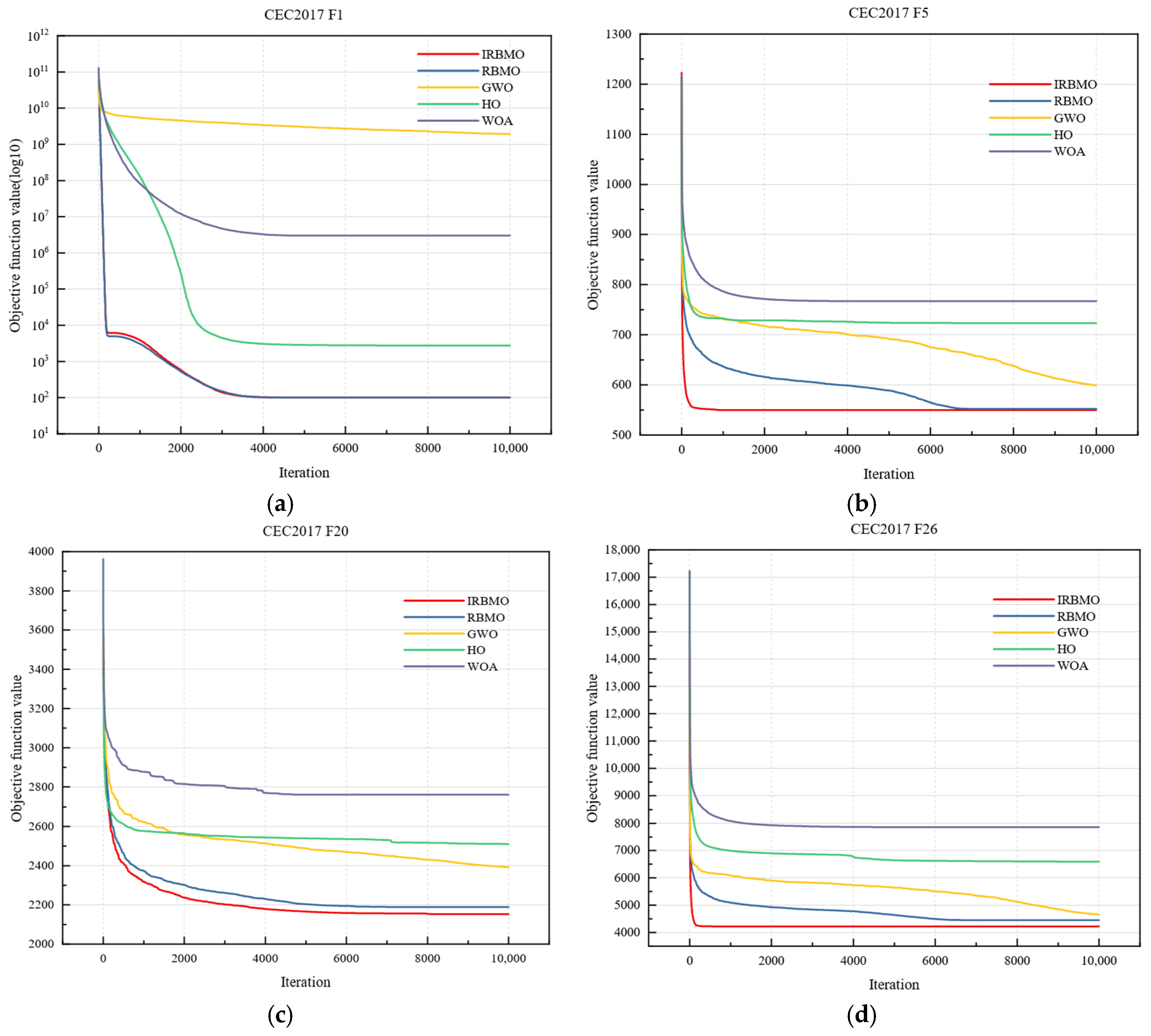
Figure 1. Convergence curves of different algorithms on CEC2017 benchmark functions: (a) F1; (b) F5; (c) F20; (d) F26.
Mathematics 14 02448 g001
Figure 2. Solution flowchart of the algorithm.
Mathematics 14 02448 g002
Figure 3. Evaluation index contribution rate values obtained by various algorithms.
Mathematics 14 02448 g003
Figure 4. Comparison of fitness function search result curves among various algorithms over 20 runs.
Mathematics 14 02448 g004
Figure 5. Mean convergence curves of different algorithms over 20 independent runs with ±1 standard deviation bands.
Mathematics 14 02448 g005
Figure 6. Evaluation flowchart of the geological environment in abandoned open-pit mines.
Mathematics 14 02448 g006
Figure 7. Location of the study area and topographic and geomorphological characteristics of the three quarries.
Mathematics 14 02448 g007
Figure 8. Combined weights of evaluation indices.
Mathematics 14 02448 g008
Figure 9. Comparison of different weight values for evaluation indices.
Mathematics 14 02448 g009
Table 1. Abandoned open-pit mine geological environment evaluation index system.
Target LayerCriterion LayerIndex LayerReferences
Abandoned open-pit mine geological environment evaluation index system [U]Geological conditions [A]Rock type [A1][30]
Hydrogeological condition [A2][44]
Topography and geomorphology [A3][31,43,45]
Earthquake intensity [A4][36]
Geological structure [A5][34]
Destruction of resources [B]Area of land damage [B1][28,42]
Exposed rock face ratio [B2][40,41]
Aquifer damage degree [B3][32]
Landscape damage rate [B4][29]
Geological environment problems [C]Comprehensive pollution degree of
water and soil [C1]
[28,33]
Scale of geological disasters [C2][41,44]
Number of geological disasters [C3][37,38]
Soil erosion [C4][28,35,38,39]
Table 2. Index-by-index comparison between the present study and the previous study.
Present StudyCorresponding Index in [28]RelationshipExplanation
Rock type [A1]Partly related to A3 Engineering geological conditionRefinedThe previous study used a broad engineering-geological condition indicator, whereas this study separately considers rock type to better reflect lithological control on rock-mass stability.
Hydrogeological condition [A2]A5 Hydrogeological conditionCommonRetained because groundwater condition is a basic factor affecting the mine’s geological environment and slope stability.
Topography and geomorphology [A3]A4 Topography and geomorphologyCommonRetained as a fundamental terrain factor influencing erosion, drainage, and restoration difficulty.
Earthquake intensity [A4]A2 Earthquake intensityCommonRetained because seismic background affects slope instability and geological hazard development.
Geological structure [A5]Partly related to A3 Engineering geological conditionRefinedGeological structure is separated from the previous broad engineering-geological condition indicator to emphasize joints, fissures, and structural control on rock-mass fragmentation.
Area of land damage [B1]B2 Land damage areaCommonRetained because land damage directly reflects reclamation workload and disturbance scale.
Exposed rock face ratio [B2]No direct counterpartNewAdded to describe exposed rock wall conditions and slope revegetation difficulty, which are important for abandoned quarry restoration.
Aquifer damage degree [B3]B3 Aquifer damageCommonRetained because mining-induced aquifer disturbance is a basic resource and environmental damage factor.
Landscape damage rate [B4]B1 Topography/landscape damage rateAdjustedRelated to the previous landscape damage indicator but expressed separately from land damage to better reflect visual landscape disturbance and ecological restoration difficulty.
Comprehensive pollution degree of
water and soil [C1]
C2 Water and soil pollutionCommonRetained because water-soil pollution is a necessary environmental problem index.
Scale of geological disasters [C2]Part of C1 Geological disasterRefinedThe previous study used one broad geological disaster indicator; this study separates the hazard scale to reflect hazard intensity and possible consequences.
Number of geological disasters [C3]Part of C1 Geological disasterRefinedAdded as an independent indicator to reflect hazard frequency and spatial distribution.
Soil erosion [C4]C3 Soil erosionCommonRetained because soil erosion is a common consequence of exposed slopes and disturbed land.
Not included in the present studyA1 Annual rainfall in [28]RemovedThe present case sites are located in the same small regional unit with limited rainfall differentiation; therefore, rainfall was not retained as an independent differentiating index
Not included in the present studyA6 Slope in [28]ReplacedSlope-related effects are reflected through topography and geomorphology, exposed rock-face ratio, and geological disaster scale/number in the present study.
Table 3. Grading criteria of the evaluation index.
Evaluation IndexGrading Criteria of Evaluation IndexType
SlightRelatively SevereSevere
A1Unweathered or slightly weatheredModerately weatheredStrongly weatheredQL
A2Uniform and stable aquiferLocally altered aquiferHighly variable aquiferQL
A3PlainLow mountains and hillsHigh mountainsQL
A4[0, 4)[4, 7](7, 12]QN
A5Simple structure and undeveloped jointsMedium structure and more developed jointsComplex structures and well-developed jointsQL
B1/h m2[0, 4)[4, 14](14, +∞)QN
B2[0, 0.2)[0.2, 0.5](0.5, 1]QN
B3No impact on production and domestic water supply in and around the mining areaPartial impact on production and domestic water supply in the mining areaImpacts the centralized water supplyQL
B4[0, 0.2)[0.2, 0.4](0.4, 1]QN
C1Pz 1 ∈ [0, 0.7)Pz ∈ [0.7, 2]Pz ∈ (2, +∞)QL
C2/104 m3[0, 1)[1, 10](10, +∞)QN
C3[0, 1)[1, 2](2, +∞)QN
C4Absent or minimal erosionLocalized or moderate erosionExtensive erosionQL
1 Pz represents the comprehensive pollution index of soil and water [33].
Table 4. Operational discrimination criteria for the three-level classification of qualitative indices.
IndexSlightRelatively SevereSevere
Rock typeDominated by hard or relatively hard rocks, the rock mass is relatively intact and slightly weathered, with poorly developed joints and fissures and the absence of distinct weak interlayers.Characterized by moderate rock strength or local presence of weak interlayers, the rock mass is moderately weathered, with relatively developed joints and fissures and local fragmentation.Dominated by soft rocks, intensely weathered rocks, or fractured rock masses, the rock mass features densely distributed joints and fissures and the presence of distinct weak interlayers or fracture zones, rendering it susceptible to collapse, rockfall, or sliding.
Hydrogeological conditionThe aquifer structure is simple, with relatively stable conditions for groundwater recharge, runoff, and discharge, and no obvious ponding or continuous seepage within the mining pit.The aquifer is locally disturbed, exhibiting seasonal seepage, local ponding, or groundwater level fluctuations, which exert a certain impact on slope stability and vegetation restoration.The aquifer structure is complex or significantly damaged, characterized by continuous seepage, ponding, or drainage difficulties within the mining pit, thereby significantly impacting slope stability, ecological restoration, or the surrounding water supply.
Topography and geomorphologyThe topographic relief is minor, the slopes are relatively gentle, and the elevation difference within the mining pit is small; the surface runoff is dispersed, presenting weak conditions for erosion and hazard development.Characterized by low mountain and hilly landforms or local steep slopes, the topographic relief is moderate; local runoff convergence and scouring are evident, possessing certain conditions for hazard development.The topography is intensely dissected, the slopes are steep, and the elevation difference is large; evident gullying or runoff convergence conditions exist, presenting strong conditions for the development of hazards such as erosion, collapse, and sliding.
Geological structureNo distinct faults, folds, or fracture zones are observed; joints and fissures are sparse, and structural planes exert a weak influence on slope stability.Joints, bedding planes, or small-scale fracture zones are locally developed, exerting a certain degree of control over local slope stability.Faults, fracture zones, or dense joints and fissures are intensely developed; the assemblage of structural planes is adverse, and the rock mass is highly fractured, exerting a pronounced control over collapses, landslides, or the instability of perilous rocks.
Aquifer damage degreeMining activities have not significantly altered the aquifer structure, groundwater recharge, runoff, and discharge conditions, or the surrounding water supply conditions.The aquifer is locally disturbed, with alterations in local groundwater emergence and discharge conditions, or exerting a minor impact on surrounding water utilization.The aquifer structure is significantly damaged, characterized by continuous drainage, water inrush, or prolonged ponding, or exerting a pronounced impact on the surrounding water supply and ecological water replenishment.
Soil erosionVegetation or surface coverage is relatively well preserved, exhibiting only minor sheet erosion or localized scouring, with a limited erosion scope.Exposed slopes are prevalent, demonstrating relatively pronounced sheet erosion, rill erosion, or localized gully erosion, with a moderate extent of soil and water loss.Extensive areas of exposed rock and soil masses, waste dumps, or high and steep slopes undergo intense scouring; gully erosion is well developed, soil and water loss is pronounced, and ecological restoration is highly challenging.
Table 5. Threshold sources and classification criteria for each evaluation index.
IndexThreshold Sources and Classification Basis
A1The classification of rock weathering degree is determined based on field geological investigations, descriptions of rock mass weathering degree, and extant research on mine geological environment evaluation.
A2The classification is determined based on relevant specifications for water supply hydrogeological investigation, and hydrogeological survey data of the study area, in accordance with aquifer stability, recharge conditions, groundwater variation characteristics, and their degree of impact on the mine geological environment.
A3Based on geomorphological type classification, topographical conditions of the study area, and extant evaluation research, geomorphological types such as plains, low mountains and hills, and high mountains are mapped to distinct geological environment impact grades.
A4Referring to seismic intensity zoning and relevant specifications, the classification is performed according to the degree of influence of seismic activity on slope stability and the formation conditions of geological hazards.
A5Based on regional geological data and field investigation results, the classification is determined according to structural complexity, joint and fissure development degree, and their impacts on rock mass stability.
B1Referring to relevant specifications in [33] and research on land damage evaluation, the classification thresholds are determined in conjunction with the actual damage scale of quarries in the study area.
B2Referring to research concerning ecological disturbance, slope revegetation, and landscape destruction in open-pit mines, classification thresholds are established in conjunction with field investigations and expert judgment.
B3Referring to relevant specifications in [33], the classification is performed according to the degree of impact of mining activities on the domestic and industrial water supply within and around the mining area, aquifer structure, and groundwater recharge conditions
B4Referring to research concerning mine landscape disturbance evaluation and ecological restoration, the classification thresholds are established in conjunction with the mine disturbance range, proportion of exposed surfaces, and degree of landscape continuity disruption within the study area.
C1Referring to the calculation and classification methodology for the comprehensive pollution index Pz in [33], the evaluation grades are delineated according to the pollution degree.
C2Referring to relevant specifications in [38], the classification thresholds are determined according to the scale and volume of the hazard mass, influence scope, and potential hazard degree.
C3Referring to relevant specifications in [38], the classification thresholds are established according to the quantity of hazard points, spatial distribution density, and governance workload.
C4Referring to relevant specifications in [38], the classification is performed according to the erosion scope, erosion intensity, slope scouring characteristics, and vegetation destruction degree.
Table 6. Elucidation on the independence of potentially correlated indices.
Potentially Correlated IndicesPotential OverlapsIndependence Explanation
C2 Scale of geological disasters/C3 Number of geological disastersBoth characterize the development of geological hazardsC2 delineates the intensity, scale, and potential hazard consequences of the hazard mass, whereas C3 characterizes the occurrence frequency and spatial distribution of hazard points. Quarries may exhibit a limited quantity of hazard masses of substantial scale, or alternatively, multiple hazard points of minor scale. Given the divergent prevention and monitoring strategies associated with each, they preclude mutual substitutability.
B1 Area of land damage/B4 Landscape damage rateBoth delineate the surface disturbance induced by mining activitiesB1 denotes the absolute area of land damage, directly correlating with the land reclamation engineering volume. B4 represents the relative proportion of landscape destruction within the mining area, reflecting the landscape pattern and the degree of ecological visual disturbance.
B2 Exposed rock face ratio/B4 Landscape damage rateBoth pertain to surface exposure and landscape degradationB2 principally delineates the degree of rock face exposure, difficulty of slope revegetation, erosion susceptibility, and natural restoration potential. B4 holistically reflects the landscape destruction intensity of the mining area.
B1 Area of land damage/B2 Exposed rock face ratioBoth are associated with land and surface destructionB1 quantifies the magnitude of damaged land necessitating reclamation, whereas B2 evaluates the proportion of exposed rock faces, which predominantly dictates the difficulty of vegetation restoration and the strategies for slope ecological restoration.
Table 7. Reference table for rk assignment.
rkExplanation
1.0Equal contribution degree between Ak−1 and Ak
1.2Slightly greater contribution degree of Ak−1 than Ak
1.4Significantly greater contribution degree of Ak−1 than Ak
1.6Extremely greater contribution degree of Ak−1 than Ak
1.8Exceptionally greater contribution degree of Ak−1 than Ak
Table 8. Test results of CEC2017 benchmark functions.
FunctionTypeIndexIRBMORBMOGWOHOWOA
Best100.000100.0003.89 × 107104.3985.50 × 105
F1unimodal functionsMean100.000100.0001.93 × 1092748.5412.98 × 106
Std8.33 × 10−57.53 × 10−51.31 × 1092542.3581.60 × 106
Best515.869523.879542.949682.076683.395
F5Simple multimodal functionsMean551.160552.257599.241723.253767.055
Std13.21416.94125.21120.88353.572
Best2010.3652028.6152141.5662322.2682366.482
F20hybrid functionsMean2188.6962152.8512392.0992510.8182760.564
Std95.70296.771151.20485.752246.298
Best2900.0002900.0004046.2622800.0282864.815
F26composition functionsMean4219.9384452.9864660.0516591.1837857.828
Std507.960550.025315.0421789.7901228.707
Table 9. Comparison of theoretical complexity and actual execution efficiency of different algorithms.
AlgorithmTime ComplexitySpace ComplexityAverage Execution TimeTime Ratio Relative to IRBMO
GWOO(TND)O(ND)0.0331 s0.24
HOO(TND)O(ND)0.4217 s3.10
WOO(TND)O(ND)0.0261 s0.19
RBMOO(TND)O(ND)0.1270 s0.94
IRBMOO(TND)O(ND)0.1360 s1.00
Table 10. Fitness function values obtained by various algorithms.
Solving MethodReference [53]GWOHOWORBMOIRBMO
Fitness function value2.14332.12332.12021.94161.77641.6941
Table 11. Statistical results of fitness function values obtained by each algorithm over 20 runs.
Solving MethodGWOHOWORBMOIRBMO
Mean2.11242.10752.09421.77321.6496
Standard Deviation0.10030.12030.11430.10050.0364
Maximum2.32022.28012.24062.11511.6941
Minimum1.95421.89211.82311.63281.5689
Table 12. Mann–Whitney U test results for fitness values.
ComparisonU Statisticp-ValueResult
IRBMO vs. GWO07.0 × 10−8Significant
IRBMO vs. HO07.0 × 10−8Significant
IRBMO vs. WO07.0 × 10−8Significant
IRBMO vs. RBMO336.67 × 10−6Significant
Table 13. Rock-mass and engineering geological characteristics of the three quarries.
QuarryQuarry AQuarry BQuarry CData Sources
Mining pit morphologyHigh, steep slopes with multiple residual mining hills on the pit floor, and the site is characterized by a concave basin configurationHigh, steep slopes with multiple residual mining hills on the pit floor, and the site is characterized by a concave basin configurationHigh, steep slopes, with an overall dip direction of approximately 105°Field investigation; engineering survey data; remote-sensing image interpretation
Topography and geomorphologyLow mountains and hillsLow mountains and hillsLow mountains and hillsTopographic map; remote-sensing image interpretation; field investigation
Exposed rock wallOne is 90 m high and 170 m long, while the other is 103 m high and 570 m longOne is 70 m high and 430 m long, while the other is 110 m high and 590 m longOne is 70 m high and 170 m long.Field investigation; engineering survey data; remote-sensing image interpretation
Rock typesSlightly weatheredSlightly weatheredModerately weatheredEngineering geological investigation report; field verification
Rock mass fragmentation characteristicsIntensely developed joints and fractures, resulting in a highly fractured rock massIntensely developed joints and fractures, resulting in a highly fractured rock massIntensely developed joints and fractures, resulting in a highly fractured rock massField geological investigation; engineering geological investigation report
Rock mass quality and slope rock mass categoryThe rock mass quality predominantly falls within Grades III-IV, and the slope rock mass primarily belongs to Classes III-IVThe rock mass quality predominantly falls within Grades III-IV, and the slope rock mass primarily belongs to Classes III-IVThe rock mass quality predominantly falls within Grades III-IV, and the slope rock mass primarily belongs to Classes III-IVEngineering geological investigation report; field investigation; expert judgment
Groundwater conditionsThe groundwater is buried at a relatively great depth, exerting a negligible influence on the engineering projectThe groundwater is buried at a relatively great depth, exerting a negligible influence on the engineering projectThe groundwater is buried at a relatively great depth, exerting a negligible influence on the engineering projectHydrogeological investigation data; engineering geological report; field investigation
Hydrogeological conditionMinor aquifer impactMinor aquifer impactMinor aquifer impactHydrogeological investigation data; engineering report; field investigation
Area of disturbed land8.8 hm27.2 hm22.8 hm2Engineering survey data; remote-sensing image interpretation
Water supply conditionsNo impact on the water supply in the mining areaNo impact on the water supply in the mining areaNo impact on the water supply in the mining areaEngineering report; field investigation
Geological hazard conditions11 collapses, with a total volume of approx. 5950 m34 collapses, with a total volume of approx. 880 m31 collapse, with a total volume of approx. 280 m3Field investigation; engineering geological investigation report
Landscape damage rate0.490.560.78Remote-sensing image interpretation; field investigation
Comprehensive soil and water pollutionMinorMinorMinorEngineering report; soil and water quality investigation data
Soil erosionSevereSevereSevereField investigation; remote-sensing image interpretation; expert judgment
Table 14. Quantitative values of evaluation indices for each quarry.
Evaluation IndicesQuarry AQuarry BQuarry C
A1112
A2111
A3222
A4777
A5333
B18.87.22.8
B20.88360.38260.4561
B3111
B40.490.560.78
C1111
C20.60.090.03
C31141
C4333
Table 15. Standardized data.
Evaluation IndicesQuarry AQuarry BQuarry C
C20.050.331
C30.090.251
A5111
A2111
B10.320.391
B3111
C4111
B20.4310.84
C1111
B410.880.63
A4111
A1110.5
A3111
Table 16. Evaluation grades of each quarry.
Quarry AQuarry BQuarry C
Membership degree values[0.405, 0.143, 0.452][0.405, 0.450, 0.145][0.742, 0.077, 0.181]
Evaluation gradesIII (Severe)II (Poor)I (Favorable)
Table 17. Parameter perturbation scheme for sensitivity analysis.
Perturbed ObjectPerturbation ModePerturbation MagnitudeCount
Expert rankingRandomly swap two adjacent indices while maintaining the overall ranking structure essentially unchanged.Adjacent swap12
rkrk = rk (1 + ε)±5%, ±10%, ±20%200
Subjective weightws = ws (1 + ε)±5%, ±10%, ±20%200
Combination coefficientαs = αs (1 + ε)±5%, ±10%, ±20%200
Membership degree conversion coefficient ββ′ = β (1 + ε)±5%, ±10%, ±20%200
Table 18. Evaluation grade stability rates under different parameter perturbations.
Perturbed ObjectPerturbation MagnitudeCountGrade Stability Rate of Quarry AGrade Stability Rate of Quarry BGrade Stability Rate of Quarry C
Expert ranking\1291.7%75%100%
Subjective weight±5%200100%100%100%
Subjective weight±10%200100%100%100%
Subjective weight±20%200100%100%100%
rk±5%200100%100%100%
rk±10%200100%89.5%100%
rk±20%20098%67%100%
Combination coefficient±5%200100%100%100%
Combination coefficient±10%200100%100%100%
Combination coefficient±20%200100%100%100%
β±5%200100%100%100%
β±10%200100%100%100%
β±20%200100%100%100%
Table 19. Mean combined weights following perturbation under different perturbation amplitudes.
IndexOriginal Combined Weights±5% Mean Weights±10% Mean Weights±20% Mean Weights
A10.052510.0525180.0523180.052011
A20.0253830.0253590.0253150.025115
A30.0242810.0242910.0241860.024245
A40.0247020.0247110.0247790.024845
A50.0265420.0265550.0265690.026413
B10.1192290.1192030.1192150.119356
B20.063090.062970.0631160.063294
B30.0253830.0253730.0251660.025514
B40.0397020.0397190.0395650.039968
C10.0253830.0254350.0254060.025461
C20.2775240.2775370.2779370.277614
C30.2707280.2708390.2707550.270802
C40.0255420.025490.025670.025363
Table 20. Comparison of evaluation results under different encoding schemes for qualitative indices.
Encoding SchemeMembership Degree Vector/Grade of Quarry AMembership Degree Vector/Grade of Quarry BMembership Degree Vector/Grade of Quarry C
1/2/3[0.405, 0.143, 0.452]/III[0.405, 0.450, 0.145]/II[0.742, 0.077, 0.181]/I
1/3/5[0.427, 0.138, 0.435]/III[0.427, 0.436, 0.137]/II[0.725, 0.103, 0.172]/I
Table 21. Comparison of evaluation grades and membership degrees among three methods.
QuarryEvaluation MethodMembership Degree ValueEvaluation Grade
AAHP-EWM-FCE[0.427, 0.121, 0.452]III
AIRMO-FAHP-EWM-FCE[0.416, 0.136, 0.448]III
AIRBMO-G1-EWM-FCE[0.405, 0.143, 0.452]III
BAHP-EWM-FCE[0.427, 0.447, 0.126]II
BIRMO-FAHP-EWM-FCE[0.416, 0.451, 0.133]II
BIRBMO-G1-EWM-FCE[0.405, 0.450, 0.145]II
CAHP-EWM-FCE[0.801, 0.047, 0.152]I
CIRMO-FAHP-EWM-FCE[0.784, 0.049, 0.167]I
CIRBMO-G1-EWM-FCE[0.742, 0.077, 0.181]I
Table 22. Comparison of membership degree differences between different methods and the proposed method.
QuarryComparative MethodEuclidean DistanceMaximum Membership Degree Difference
AThe Proposed Method and AHP-EWM-FCE0.0310.022
AThe Proposed Method and IRMO-FAHP-EWM-FCE0.0140.011
BThe Proposed Method and AHP-EWM-FCE0.0290.022
BThe Proposed Method and IRMO-FAHP-EWM-FCE0.0170.012
CThe Proposed Method and AHP-EWM-FCE0.0730.059
CThe Proposed Method and IRMO-FAHP-EWM-FCE0.0520.042
Table 23. Engineering management implications of evaluation results for the three quarries.
QuarryEvaluation GradeRemediation PriorityManagement ImplicationRecommended Restoration Measures
AIIIHighGeological environment issues are relatively prominent, indicating high remediation urgencyClearance of unstable rocks, slope cutting and load reduction, slope protection, interception and drainage, topsoil covering, and revegetation
BIIMediumCertain degradation and risks exist, necessitating focused monitoring and localized remediationLocalized slope reinforcement, drainage system improvement, restoration of exposed surfaces, and regular inspection
CILowGeological environment quality is relatively favorable, with primary emphasis on maintenance and restorationVegetation maintenance, routine monitoring, soil and water conservation, and ecological restoration
Disclaimer/Publisher’s Note: The statements, opinions and data contained in all publications are solely those of the individual author(s) and contributor(s) and not of MDPI and/or the editor(s). MDPI and/or the editor(s) disclaim responsibility for any injury to people or property resulting from any ideas, methods, instructions or products referred to in the content.