Abstract
Connectivity is one of the essential needs in today’s standards in many aspects of life, starting with personal relationships, education, and remote work and ending with the security and economy of countries. However, connectivity is susceptible to intentional and unintentional disruptions, leading to great impact on critical infrastructures. Hence, maintaining connectivity is a crucial task to sustain the continuous flow of life. The challenge is to find an optimal recovery plan to reconnect all demands as soon as possible after the disruptive event, ensuring fairness in the process of reallocating the remaining resources. In this paper, we present a post-disruption recovery framework for networked systems to optimize the recovery plan to reconnect the network demands as soon as possible. More specifically, we introduce an algorithmic approach using a mathematical programming model that optimally recovers the disrupted arcs of the network while ensuring the highest connectivity. The proposed approach considers both fairness and efficiency through finding the MMF (max-min fairness) resource allocation throughout the recovery process. The proposed approach is tested on a variety of benchmark networks under a set of disruption levels; then, the results are compared with the maximum-flow model.
Keywords:
max-min fairness; the direct progressive-filling algorithm; load balancing; goal programming; fairness in resource allocation MSC:
90C11; 90C29; 90C47; 90C90; 91B32
1. Introduction
Critical infrastructure systems, including energy grids, water supply networks, transport corridors, and communications backbones, are the essential machinery that sustains modern life. They enable economic vitality, social stability, and national security, yet their importance often becomes most visible in moments of disruption. These systems are capital-intensive and inherently vulnerable to a wide spectrum of hazards, ranging from natural disasters to intentional attacks [1,2,3]. In addition, the growing interconnection among infrastructure networks, where electricity powers pumping stations, transport facilitates fuel distribution, and telecommunications support all other services, creates fragility. A failure in one system can cascade into others, producing widespread consequences [4,5,6,7,8].
Connectivity is particularly crucial in this context. It represents one of the essential needs of modern society, extending from personal communications and education to emergency response and national economies. Connectivity, however, is vulnerable to intentional and unintentional disruptions that can have severe consequences on critical infrastructures such as social media, transportation, and emergency services. Hence, maintaining and restoring connectivity is fundamental to sustaining the continuous flow of life, either by mitigation or resilience. Mitigation can be utilized to reduce the severity, impact, or risk on the communication network before the damaging event occurs, thus enabling prompt recovery. On the other hand, resilience refers to the ability of a network to endure a disruption and recover from it back to the original level of performance [9], which can be measured by different approaches that are investigated in the literature [10].
In this study, we adopt the framework illustrated in Figure 1, originally introduced by [11], which evaluates network resilience using a performance-based function. As shown in the figure, resilience is characterized along two primary dimensions: vulnerability, referring to the extent of performance degradation caused by a disruption [12], and recoverability, denoting the rate at which the network returns to a target performance level [13]. These dimensions are assessed over time across three key states, namely the original, disrupted, and recovered phases, using the performance function .
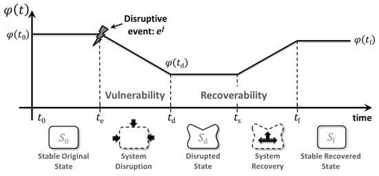
Figure 1.
A depiction of a performance function of a network through different transition states over time (adopted [11]).
Henry and Ramirez-Marquez [11] defined network resilience, denoted as Я, as the ratio of a system’s recovered performance to the maximum loss experienced following a disruptive event , with representing the set of all possible disruptions. Mathematically, resilience at time is given by Equation (1), where the numerator quantifies the performance regained after the disruption, and the denominator captures the total degradation in performance from the original state at time to the disrupted state at time , where .
As defined in Equation (1), the resilience metric ranges between 0 and 1, with a value of 1 signifying that the network has fully recovered to its pre-disruption performance level. In this study, resilience is assessed using two performance indicators: maximum flow and the number of connected nodes. Of the many pillars of resilience, restoration is perhaps the most tangible where plans confront reality [14,15,16]. Restoration is not simply “repair”. It is an orchestrated effort to bring essential services back to acceptable levels under intense pressure, in environments where information is imperfect, conditions are unstable, and resources crews, equipment, and budgets are lacking [17,18,19].
Within the broader concept of resilience, restoration is perhaps the most tangible pillar where planning meets reality. Making restoration decisions in such contexts is rarely straightforward. In an interdependent system, one sequence of repairs may be technically possible but strategically flawed because it ignores procedural dependencies [7,8]. Clearing a blocked arterial road may be useless if live power lines still hang across it. Yet, repairing those lines may require access through the very road that remains blocked. This interplay between systems is often where restoration falters not for lack of will but for lack of coordination [14]. Historically, restoration planning has leaned heavily on optimization models that privilege efficiency to maximize total flow and minimize aggregate cost [3,7,14,20,21,22,23]. Such objectives are important, but they have their blind spots. Efficiency alone can lead to inequitable outcomes, with high-demand or central nodes restored quickly, while peripheral or less affluent areas wait far longer. Even approaches such as concurrent restoration repairing several components in parallel do not inherently solve this imbalance unless fairness is built in from the outset [24].
Here, the concept of MMF offers a principled alternative. MMF seeks to elevate the least-served demands first, progressively narrowing disparities until no further gain can be made for one without harming another [24,25]. While this idea has deep roots in fields like telecommunications, its practical integration into critical infrastructure restoration has been limited. The reasons are not trivial. Modeling such priorities under real-world constraints is technically demanding, particularly when interdependencies complicate every scheduling decision [26].
The work presented in this paper focuses on fairness in restoration, which remains an underexplored yet critical aspect of post-disruption recovery planning. We introduce a novel framework that adopts the MMF principle, which prioritizes fairness while still utilizing available resources to achieve high overall efficiency. At the core of our approach lies the direct progressive-filling algorithm (DPFA), a new algorithm that, to the best of our knowledge, has not been previously applied in this context. The DPFA begins by restoring the links associated with the least-served demands to reestablish connectivity for as many users as early as possible. It employs a goal programming formulation with two objectives: the first aims to maximize the flow for non-saturated demands until constrained, and the second identifies which demands are saturated in each iteration. This framework is evaluated on benchmark interdependent infrastructure networks under varying disruption levels and compared against a conventional maximum-flow model. The maximum-flow model is chosen to be compared with MMF because it represents one of the most common objectives in flow networks, alongside cost minimization. While other fairness-based approaches can be considered, the notion of fairness is subjective and varies based on the objective. MMF stands out as the only fairness criterion with a clear, well-defined linear formulation compared to other schemes. Hence, other fairness approaches require non-linear modeling. The results reveal how fairness-oriented planning can significantly improve both the distribution and speed of recovery. The paper proceeds as follows: Section 2 surveys the literature on infrastructure restoration and fairness in resource allocation. Section 3 details the mathematical formulation of the maximum-flow restoration model. Section 4 discusses DPFA and its mathematical formulation. Section 5 reports on the numerical experiments and results. We conclude in Section 6 with remarks on broader applicability and directions for future research.
2. Literature Review
In this section, a literature review is presented regarding restoration of networks, fairness in resource allocation, and then fair restoration.
2.1. Network Restoration
Interdependencies among infrastructure networks can be classified into four categories [27]: (i) physical, where an output from a network is an input to another one and vice versa; (ii) cyber, involving dependence on information transmitted through an information infrastructure; (iii) geographical, where networks are affected by the same local disruptive event; and (iv) logical interdependencies, which include all other types of interdependencies. Several studies in the literature have addressed the problem of the restoration of a system of interdependent infrastructure networks after a disruptive event. Accordingly, different approaches have been proposed with different objectives: (I) determining the set of disrupted network components to be restored (e.g., [28]), (II) scheduling a predetermined set of disrupted network components (e.g., [29]), or (III) an integration of objectives (I) and (II), i.e., prioritizing the restoration of the disrupted components and assigning and scheduling them to the available resources (e.g., [21]).
For instance, ref. [8] proposed a model that seeks to minimize total disruption, repair, and flow costs by identifying which components to restore, determining their repair modes, assigning them to crews for individual or concurrent work, and establishing baseline restoration sequences across scenarios. Similarly, ref. [21] formulated the restoration decision problem as the task of identifying a combined repair sequence that minimizes the overall loss of resilience. In addition, ref. [30] aimed to determine optimally which disrupted links should be restored and in what sequence through a mixed-integer nonlinear programming (MINLP) model combined with a novel metaheuristic method to provide robust and efficient solutions.
Building on these efforts, ref. [20] introduced a heuristic-based dispatching rule to support decision making in both network design and scheduling, while [31] presented a multi-objective mixed-integer linear programming model that optimizes task sequencing and crew allocation in interdependent infrastructure networks. Their approach also identifies points where additional resources can accelerate restoration. Furthermore, a generalized form of integrated network design and scheduling problems that incorporates multiple scheduling features, particularly in the context of infrastructure and supply chain restoration, was proposed in [32]. These features include release dates, flexible release times, and machines capable of performing multiple functions. However, such studies focused on objectives other than fairness in restoration, which is the focus of this study.
2.2. Fairness in Resource Allocation
Fairness has been gaining tremendous interest in the past few years. Fairness in restoration is usually overlooked because the focus is primarily centered around other objectives such as efficiency, resilience, or profitability. Fairness is implemented in a few applications in communication networks (see [33,34] for fairness in resource allocation). MMF is a widely implemented scheme (if not the most) in fair resource allocation, and the progressive-filling algorithm (PFA) is the well-known approach to achieve it [35]. PFA prioritizes the lower demands (users of the network) to allocate as equal resources as possible to all demands. The weakness of the PFA is that it depends on complementary slackness in identifying the set of blocking demands to be excluded in the next iterations. Hence, this algorithm cannot be used in network restoration due to its non-convex structure. Another algorithm called binary search uses a different approach to identifying the blocking demands, but it requires a limitation of access rates for the algorithm to work [36]. Ref. [37] proposed a multi-objective optimization function that finds the optimal quality of service (QOS) and network efficiency simultaneously to find the fairest allocation as possible. Ref. [34] introduced a distributed algorithm to find fair and dynamic optimal transport, where every pair of suppliers and receivers compute their solution and update the transport strategy through iterative negotiation in a decentralized manner.
Fairness in resource allocation has been explored in the literature in a wide range of applications, such as communication networks, facility location, evacuation and traffic management, air traffic control, and job scheduling. These studies use a variety of fairness measures, such as basic statistical measures, the Gini index, Jain’s index, and unfairness [38,39,40,41]. Basic statistical measures such as mean, median, and variance provide a reliable indication of how resources are distributed among the demands. Additional measures were discussed by [42], such as the maximum of absolute deviations (MAD), the sum of squared deviations (SSD), and the sum of absolute deviations (SAD). These measures can be set as objectives in the mathematical programming models. Nevertheless, they may result in poor efficiency since they do not exploit unused resources. The SAD measure is used as a measure of fairness for comparison purposes.
Ref. [40] developed a function called the Gini index to measure the income inequality of a society. The Gini index ranges between 0 and 1, with 0 for perfect equality and 1 for an individual receiving income when all other individuals do not receive any income. Ref. [39] developed a function derived from the coefficient of variation (COV) that ranges from 1/n to 1, given that the higher the index, the fairer the resource distribution. The unfairness measure is a fraction of the maximum difference between the highest and the lowest resources assigned, given that the lower bound is 1, indicating complete fairness of resource distribution [38]. The common drawback of these measures is that they are non-linear functions, so they cannot be used either as objective functions or as constraints in MIP models unless they are linearized. In our study, we might use any of these measures to compare the fair resource allocation solution with solutions from other conventional methods. The approach this paper adopts is MMF, which does not pursue perfect fairness of resource allocation, as it prioritizes fairness and then utilizes the unused resources to achieve both fairness and high utilization of resources. Price of fairness (POF) measures the percentage of loss of utilization after incorporating fairness in the model to indicate the impact of fairness on the overall efficiency of the system [43]. The POF value ranges between zero and one, where zero indicates no loss of efficiency when fairness is implemented, and one indicates all efficiency is compromised to implement fairness.
2.3. Fair Network Restoration
Despite the significance of fairness in network restoration, it has not been extensively explored in the literature. Ref. [26] used the Kolm–Pollak equally distributed equivalent (EDE) measure to reflect the restoration inequalities across a system. For every possible restoration strategy, the EDE measure is calculated for the recovered network performance distribution to select the fairest restoration strategy for specific nodes or for the overall network. Ref. [25] proposed two bi-objective models to balance conflicting objectives by integrating graph signal processing, fairness, and cost in these models. Another study introduced a multi-objective fair distribution and restoration model for enhanced resilience of supply chain transportation networks [24]. This study proposes a multi-objective non-linear mixed integer programming to restore disruptions while maximizing the supply chain network performance in transportation networks. Ref. [44] investigated the enhancement of resilience of supply chain networks during disruptions through studying the effectiveness of two fairness-based distribution approaches.
3. The Maximum-Flow Restoration Model
In this section, we discuss the maximum-flow model that restores the network connectivity under the objective of maximizing flow without considering the individual demands in the network. We have the network graph with the set of nodes , the set of directed arcs , and each arc , where and . and are the supply and terminal nodes of the demand , respectively, given that is the supply node. set, and is the terminal node set, where and . The source node set , and the terminal node as seen in Table 1.

Table 1.
Sets, parameters, and decision variables of the maximum-flow restoration model.
The objective of the maximum-flow restoration model (3) is to maximize the flow for all demands at all time periods. The set of constraints (4) represent the flow conservation constraints, where node is (i) a terminal node if the incoming flow is greater than the outgoing flow at node, (ii) a source node if the outgoing flow is greater than the incoming flow at node, and (iii) a transshipment node if the incoming and outgoing flows are equal at node. Each demand flows in an independent network; however, the set of capacity constraints (5) links all the demand flows to one network sharing the same capacity resource, which ensures that all the demand flows pass through the arc but do not exceed its capacity. The set of constraints (6) allows the link to send flow after time when the link is fixed at time t in the set of constraints (7). The set of constraints (8) measures the difference in flow between demands as a measure of fairness, as seen in Equation (2). The set of constraints (9) and (10) denotes the nature of the decision variables.
4. The Fair Restoration Model
In this section, we utilize the new algorithm, called the direct progressive-filling algorithm (DPFA), to find the MMF restoration procedure. This approach has not been explored yet to the best of our knowledge. This starts with restoring the links that affect the lower or least fortunate demands to bring back connectivity to as many demands as soon as possible. The algorithm relies on a goal programming approach to achieve MMF.
4.1. The Direct Progressive Filling Model
We have the network graph with the set of nodes , the set of directed arcs , and each arc a , where and N. and are the supply and terminal nodes of the demand , respectively, given that is the supply node set, and is the terminal node set, where and . The source node set , and the terminal node (Table 2 and Table 3).
Table 2.
Sets and parameters of the maximum-flow restoration model.
Table 3.
Decision variables of the maximum-flow restoration model.
The model has two objectives (11 and 12). The first objective (11) is to maximize the flow for non-saturated demands simultaneously until blocked by a constraint or a set of constraints, and the second objective (12) is used to detect the saturated demands. The algorithm relies on goal programming to identify the set of saturated demands. Hence, the model is composed of hard and soft constraints. The set of constraints (13) represent the flow conservation constraints, where node is (i) a terminal node if the incoming flow is greater than the outgoing flow at node , (ii) a source node if the outgoing flow is greater than the incoming flow at node , and (iii) a transshipment node if the incoming and outgoing flows are equal at node . Each demand flows in an independent network ; however, the set of capacity constraints (14) links all the demand flows to one network sharing the same capacity resource, which ensures that all the demand flows pass through the arc but do not exceed its capacity. The set of soft constraints (15) can detect the saturated demands when the negative deviational variables are minimized in the second objective (12). Note that in the second objective, only the non-blocking constraints’ negative deviations are minimized with the help of the indicator parameter . It is worth mentioning that being able to minimize the negative deviational variable of the demand to zero indicates that the corresponding demand is non-saturated; hence, it is improvable in the next iteration. More details are in the next section. The set of constraints (16) maximizes the flow of only non-saturated demands with the help of the parameter . The saturated demands are excluded from the maximization process because it removes the lower bound if the parameter equals 1, given that M is a sufficiently large number. The set of constraints (17) sets a permanent lower bound for the saturated demands. The set of constraints (18) allows the link to send flow after the time t when the link is fixed at time t in the set of constraints (19). The set of constraints (20) is used as a measure of fairness, as seen in Equation (2). The set of constraints (21) and (22) denotes the nature of the decision variables.
4.2. The Direct Progressive-Filling Algorithm (DPFA)
The procedure of the DPFA is illustrated in this section using the model (11)–(22).
To initialize the algorithm, the iteration number is set to 0, the saturated demands parameter is set to 0 for all demands, and the lower bound is set to 0 for all demands, as seen in Algorithm 1. In the first iteration, step 2, the total flow is maximized until a set of saturated demands is reached. In step 3, problem is solved to identify the saturated demands. An is added on top of the maximum flow to be set as , then the negative deviation from of every demand is minimized as seen in constraint (15) through the objective function (12). The M and values used for all examples and experiments in this article are set to and , respectively. The value of M is set to greater than or equal to the maximum capacity of the links so it can compensate for the difference if some demands are assigned 0 flow and other demands assigned full-capacity flow. On the other hand, the is set to less than or equal to the minimum difference in flow between the sets of saturated demands (we call it . The value is set significantly lower than the minimum difference because it might not be known in advance. The could be thought of as the accuracy of the output if it exceeded the value. In that case, the algorithm might stop prematurely, and the output becomes an approximation to the MMF. However, we will still obtain an MMF solution if the is sufficiently small. Setting different values of is illustrated through examples 1 and 2. The demand is considered improvable if the negative deviation is minimized to zero, and it is considered saturated demand otherwise. In this step, the set of saturated demands is identified, and their parameter is set to 1. The weight used for tie-breaking in the case of non-convex discrete problems gives priority to specific demands in the second optimization problem, , after maximizing all demand flows in the first problem, . This emphasizes fairness where all demands are treated equally in the first part of optimization, and then, priorities are activated in the second part of optimization when the blocking state is reached. The process is repeated by going back to step 2 until all demands are set as saturated demands. See Figure 2 for more illustration.
| Algorithm 1: The DPFA algorithm for finding MMF resource allocation and the associated flow vector | |
| Step 1 | Set , , and |
| Step 2 | If , stop. Otherwise, set and find the maximum by solving the problem |
| Step 3 | If , set and |
| Step 4 | solve the problem |
| Step 5 | if , set |
| Step 6 | Go to step 2 |
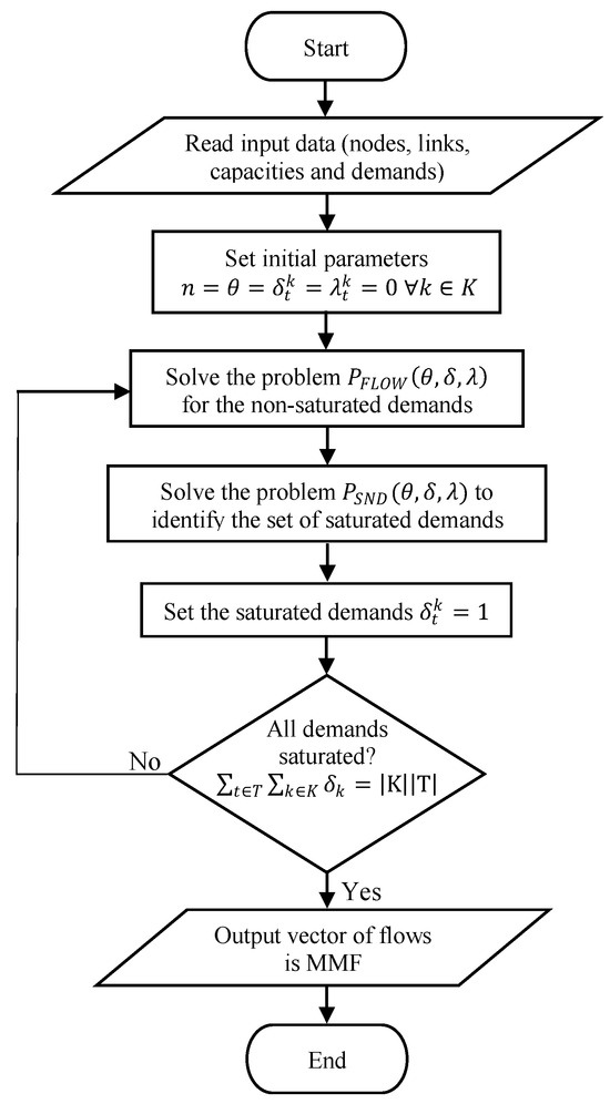
Figure 2.
The flow chart of the DPFA algorithm.
5. Numerical Experiments
The DPFA is tested on a variety of benchmark networks, as seen in Figure 3. The benchmark networks are acquired from the survivable fixed telecommunication network design library (SNDlib) established by Orlowski et al. [45]. The SNDlib provides realistic telecommunication network data available to the research community for testing and comparison. These benchmark networks are of different sizes in terms of nodes, arcs, and demands. The algorithm is used to find the optimal restoration strategy. Hence, we assume that each network undergoes different disruption sizes ranging from 10% to 40%. These disruption sizes cover a wide range of potential disruption levels, ranging from minor to severe ones.
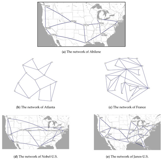
Figure 3.
The five considered networks are Abilene, Atlanta, France, Nobel-U.S., and Janos-U.S.
The networks tested are listed in Table 4 given the number of nodes |N|, the number of arcs |A|, and the number of network demands |K|. The capacity of each arc is assumed to be 1000 MB/s, and each arc is bidirectional for all networks.
Table 4.
The network properties.
The results of the DPFA are compared with the maximum-flow model in terms of connectivity, total flow, average fairness, and computational time. These measures are highlighted since they play a critical role in disasters. The most important measure is connectivity since it measures the average percentage of demands connected during the full disruption and in every stage of recovery, assuming that a user must receive at least 0.256 MBPS to be considered as connected based on the International Telecommunication Union (ITU). The other measure is the total flow of bandwidth in the network because it indicates the average amount of bandwidth flow after a full disruption and during every stage of recovery. The fairness measure is an additional indicator of how the bandwidth is allocated fairly among the network demands. Although the DPFA allocates resources in an MMF scheme, additional fairness measures provide more insight and measure the difference between the tested approaches.
Firstly, the networks are tested using the maximum-flow model with the objective of maximizing the flow in every recovery stage. The summary of results is illustrated in Table 5 for every network, disruption level, and number of disrupted arcs, including a set of performance measures. The performance measures are the average flow, average connected demands, and average fairness during the recovery process from the time of disruption to the recovery of the last disrupted arc. The average fairness and average flow are very large numbers, so they are scaled to be from 0 to 1. To scale the average flow, it is divided by the maximum flow possible in the network, given that 0 indicates no flow and 1 the maximum flow possible. To scale the average fairness, it is divided by the worst fairness value recorded in both objectives (maximum flow and MMF flow), given that 0 indicates complete fairness, and 1 is the worst recorded fairness. Note that the average flow decreases with the size of disruption, which is logical when more arcs are disrupted, leading to less flow in the network. The average fairness measure performs poorly in the maximum-flow model because its value is close to 1 in most disruption levels for all networks since this model does not consider fairness in the resource allocation process. In addition, the average number of connected demands is 0.85 for all networks and all disruption levels, indicating that 0.15 of the demands are not connected on average.
Table 5.
The maximum-flow model results.
The summary of the MMF results is illustrated in Table 6, including every disruption level for each tested network in addition to the number of disrupted arcs and the performance measures used for comparison. Note that the average flow decreases with the size of disruption, which is logical when more arcs are disrupted, leading to less total flow in the network. The average fairness measure decreases with the size of the disruption since the demands that are used to receive higher bandwidth receive less bandwidth because of fairness. To illustrate, the demands that receive higher bandwidth will receive less after disruption because part of this bandwidth is assigned to the demands that do not receive any bandwidth after disruption since the flow is MMF. This allocation results in more connected demands compared to other objectives compared to the maximum-flow model. Note that all demands are connected in most disruption levels when the DPFA is used, with an average of 0.98. The drawback of this approach is that it requires multiple iterations that increase with the size of the disruption and the size of the network, leading to a higher computational time compared to the maximum-flow model. Also, the average price of fairness (POF) is computed for every disruption to measure how much flow is compromised to achieve the MMF, given that 0 means no flow has been compromised to achieve MMF, and 1 means all the flow is compromised to achieve MMF.
Table 6.
The MMF model results.
The charts in Figure 4 elaborate on the connectivity and the flow for the Abilene network for each disruption level. Note that when the disruption level is 10%, the network is still capable of withstanding this disruption and keeps all demands connected when using the MMF model. On the other hand, the MF model results in connectivity loss of almost 30% of the demands in the first time period, as seen in Figure 4A. The difference in flow in not considerable, as seen in Figure 4B, when implementing fairness in comparison to the maximum flow. When the disruption level is 20%, the MMF recovers the connectivity in one time period, while the MF model requires four time periods to recover the connectivity, as seen in Figure 4C, and the difference in flow is minimal, as seen in Figure 4D. This is similar to the remaining disruption levels showing that the MMF recovers the disconnected demands in a minimal number of time periods. More charts can be found in the Figure 5 and Appendix A (Figure A1, Figure A2 and Figure A3).
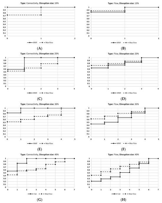
Figure 4.
The results of the Abilene network given that (A) is the connectivity of disruption size 10%, and (B) is the flow of the disruption size 10%. (C) is the connectivity of disruption size 20%, and (D) is the flow of disruption size 20%. (E) is the connectivity of disruption size 30%, and (F) is the flow of disruption size 30%. (G) is the connectivity of disruption size 40%, and (H) is the flow of disruption size 40%.
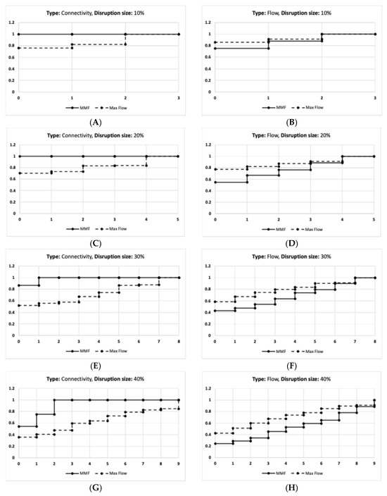
Figure 5.
The results of the Atlanta network given that (A) is the connectivity of disruption size 10%, and (B) is the flow of the disruption size 10%. (C) is the connectivity of disruption size 20%, and (D) is the flow of disruption size 20%. (E) is the connectivity of disruption size 30%, and (F) is the flow of disruption size 30%. (G) is the connectivity of disruption size 40%, and (H) is the flow of disruption size 40%.
The computational time is illustrated for each network and disruption level in both the maximum-flow and MMF models, as seen in Table 5 and Table 6. Note that the computational time is affected by both the network size and the disruption level. The computational complexity of the classical network flow model developed by Ford–Fulkerson is , given , , and , which is polynomial [46,47]. Adding binary variables makes it NP-hard. The computational complexity of the maximum-flow model is , where is the number of disrupted arcs, and the computational complexity for the DPFA model is , where is the number of iterations.
The price of fairness is calculated in every stage of the recovery for all networks. Note that the price of fairness depends on the network structure. Figure 6 represents the worst scenario in all tested networks when the POF reaches 0.5 when 40% of the network is disrupted, and Figure 7 represents the best scenario among the tested networks when the maximum POF reaches 0.14 when 40% of the network is disrupted. Note that the POF is lower when fewer arcs are disrupted.
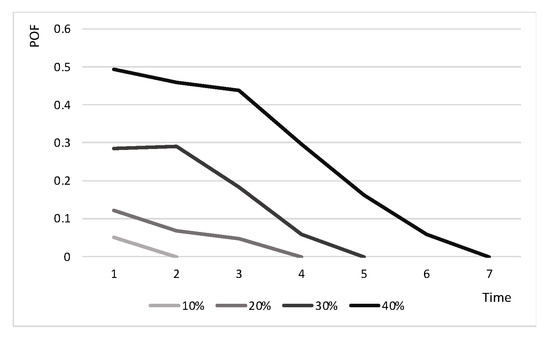
Figure 6.
The POF for the Abilene network under all disruption levels.
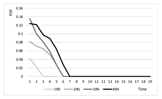
Figure 7.
The POF for the France network under all disruption levels.
6. Concluding Remarks
To conclude, this study proposes an algorithmic approach that can find the MMF network restoration plan through the DPFA. A variety of benchmark networks are tested to illustrate the benefit of implementing the MMF concept on restoration. We found that the algorithm attempts to connect all network demands from the first stage of restoration, and it finds the maximum possible number of connected users in every stage. The algorithm also attempts to find the maximum flow in every restoration stage while prioritizing fairness. Through the POF, we can observe that the algorithm does not compromise a considerable amount of flow to achieve the MMF. One drawback of this algorithm is it requires multiple iterations to find the MMF solution, which leads to a higher computational time in addition to the NP-hard complexity of this problem.
As for future work, there are several possible extensions for the developed models.
- Future work should develop a formulation capable of identifying the placement of recovery resources in a manner that remains robust against a wide range of disruptions with differing probabilities (facility location);
- It is essential to examine recovery in relation to both community resilience and the geographic distribution of vulnerable populations;
- Future work could incorporate stochastic programming or robust optimization techniques to model uncertainty in disruption magnitude, repair durations, and resource accessibility.
Author Contributions
Conceptualization, H.S.B.O. and Y.A.A.; methodology, H.S.B.O.; software, H.S.B.O.; validation, H.S.B.O. and Y.A.A.; formal analysis, H.S.B.O. and Y.A.A.; writing—review and editing, H.S.B.O., Y.A.A. and M.A.; visualization, H.S.B.O. All authors have read and agreed to the published version of the manuscript.
Funding
This research received no external funding.
Data Availability Statement
The data are available at https://sndlib.put.poznan.pl/home.action, accessed on 19 November 2024.
Acknowledgments
The authors gratefully acknowledge the maintainers of the SNDlib repository for providing the benchmark data used in this study.
Conflicts of Interest
The authors declare that there are no conflicts of interest.
Appendix A


Figure A1.
The results of the France network given that (A) is the connectivity of disruption size 10%, and (B) is the flow of the disruption size 10%. (C) is the connectivity of disruption size 20%, and (D) is the flow of disruption size 20%. (E) is the connectivity of disruption size 30%, and (F) is the flow of disruption size 30%. (G) is the connectivity of disruption size 40%, and (H) is the flow of disruption size 40%.


Figure A2.
The results of the Nobel—U.S. network given that (A) is the connectivity of disruption size 10%, and (B) is the flow of the disruption size 10%. (C) is the connectivity of disruption size 20%, and (D) is the flow of disruption size 20%. (E) is the connectivity of disruption size 30%, and (F) is the flow of disruption size 30%. (G) is the connectivity of disruption size 40%, and (H) is the flow of disruption size 40%.


Figure A3.
The results of the Janos—U.S. network given that (A) is the connectivity of disruption size 10%, and (B) is the flow of the disruption size 10%. (C) is the connectivity of disruption size 20%, and (D) is the flow of disruption size 20%. (E) is the connectivity of disruption size 30%, and (F) is the flow of disruption size 30%. (G) is the connectivity of disruption size 40%, and (H) is the flow of disruption size 40%.
References
- Sun, J.; Zhang, Z. A post-disaster resource allocation framework for improving resilience of interdependent infrastructure networks. Transp. Res. Part D Transp. Environ. 2020, 85, 102455. [Google Scholar] [CrossRef]
- Fang, X.; Lu, L.; Li, Y.; Hong, Y. A Driver-Pressure-State-Impact-Response study for urban transport resilience under extreme rainfall-flood conditions. Transp. Res. Part D Transp. Environ. 2023, 121, 103819. [Google Scholar] [CrossRef]
- Peng, Y.; Xu, M.; Li, G.; Chen, A. Sequencing post-disruption concurrent restoration via a network flow approach. Transp. Res. Part D Transp. Environ. 2024, 133, 104234. [Google Scholar] [CrossRef]
- Ouyang, M. Review on modeling and simulation of interdependent critical infrastructure systems. Reliab. Eng. Syst. Saf. 2014, 121, 43–60. [Google Scholar] [CrossRef]
- Eusgeld, I.; Nan, C.; Dietz, S. “System-of-systems” approach for interdependent critical infrastructures. Reliab. Eng. Syst. Saf. 2011, 96, 679–686. [Google Scholar] [CrossRef]
- Buldyrev, S.V.; Parshani, R.; Paul, G.; Stanley, H.E.; Havlin, S. Catastrophic cascade of failures in interdependent networks. Nature 2010, 464, 1025–1028. [Google Scholar] [CrossRef]
- Karakoc, D.B.; Almoghathawi, Y.; Barker, K.; González, A.D.; Mohebbi, S. Community resilience-driven restoration model for interdependent infrastructure networks. Int. J. Disaster Risk Reduct. 2019, 38, 101228. [Google Scholar] [CrossRef]
- Alkhaleel, B.A.; Liao, H.; Sullivan, K.M. Model and solution method for mean-risk cost-based post-disruption restoration of interdependent critical infrastructure networks. Comput. Oper. Res. 2022, 144, 105812. [Google Scholar] [CrossRef]
- Barker, K.; Lambert, J.H.; Zobel, C.W.; Tapia, A.H.; Ramirez-Marquez, J.E.; Albert, L.; Nicholson, C.D.; Caragea, C. Defining resilience analytics for interdependent cyber-physical-social networks. Sustain. Resilient Infrastruct. 2017, 2, 59–67. [Google Scholar] [CrossRef]
- Hosseini, S.; Barker, K.; Ramirez-Marquez, J.E. A review of definitions and measures of system resilience. Reliab. Eng. Syst. Saf. 2016, 145, 47–61. [Google Scholar] [CrossRef]
- Henry, D.; Ramirez-Marquez, J.E. Generic metrics and quantitative approaches for system resilience as a function of time. Reliab. Eng. Syst. Saf. 2012, 99, 114–122. [Google Scholar] [CrossRef]
- Jönsson, H.; Johansson, J.; Johansson, H. Identifying critical components in technical infrastructure networks. Proc. Inst. Mech. Eng. Part O J. Risk Reliab. 2008, 222, 235–243. [Google Scholar] [CrossRef]
- Rose, A. Economic resilience to natural and man-made disasters: Multidisciplinary origins and contextual dimensions. Environ. Hazards 2007, 7, 383–398. [Google Scholar] [CrossRef]
- Saha, N.; Rezapour, S.; Sahin, N.C.; Amini, M.H. Coordinated restoration of interdependent critical infrastructures: A novel distributed decision-making mechanism integrating optimization and reinforcement learning. Sustain. Cities Soc. 2024, 114, 105761. [Google Scholar] [CrossRef]
- Wei, Y.; Cheng, Y.; Liao, H. Optimal resilience-based restoration of a system subject to recurrent dependent hazards. Reliab. Eng. Syst. Saf. 2024, 247, 110137. [Google Scholar] [CrossRef]
- Almoghathawi, Y.; Selim, S.; Barker, K. Community structure recovery optimization for partial disruption, functionality, and restoration in interdependent networks. Reliab. Eng. Syst. Saf. 2023, 229, 108853. [Google Scholar] [CrossRef]
- Dou, Q.; Lu, D.G.; Zhang, B.Y. Physical resilience assessment of road transportation systems during post-earthquake emergency phase: With a focus on restoration modeling based on dynamic Bayesian networks. Reliab. Eng. Syst. Saf. 2025, 257, 110807. [Google Scholar] [CrossRef]
- Yang, Y.; Li, Z.; Lo, E.Y. Multi-timescale risk-averse restoration for interdependent water-power networks with joint reconfiguration and diverse uncertainties. Reliab. Eng. Syst. Saf. 2025, 261, 111083. [Google Scholar] [CrossRef]
- Alkhaleel, B.A.; Liao, H.; Sullivan, K.M. Risk and resilience-based optimal post-disruption restoration for critical infrastructures under uncertainty. Eur. J. Oper. Res. 2022, 296, 174–202. [Google Scholar] [CrossRef]
- Nurre, S.G.; Cavdaroglu, B.; Mitchell, J.E.; Sharkey, T.C.; Wallace, W.A. Restoring infrastructure systems: An integrated network design and scheduling (INDS) problem. Eur. J. Oper. Res. 2012, 223, 794–806. [Google Scholar] [CrossRef]
- Xu, M.; Li, G.; Chen, A. Resilience-driven post-disaster restoration of interdependent infrastructure systems under different decision-making environments. Reliab. Eng. Syst. Saf. 2024, 241, 109599. [Google Scholar] [CrossRef]
- Ouyang, M.; Wang, Z. Resilience assessment of interdependent infrastructure systems: With a focus on joint restoration modeling and analysis. Reliab. Eng. Syst. Saf. 2015, 141, 74–82. [Google Scholar] [CrossRef]
- Zhang, Q.; Nie, Y.; Du, Y.; Zhao, W.; Cao, S. Resilience-based restoration model for optimizing corrosion repair strategies in tunnel lining. Reliab. Eng. Syst. Saf. 2025, 253, 110546. [Google Scholar] [CrossRef]
- Abushaega, M.M.; González, A.D.; Moshebah, O.Y. A fairness-based multi-objective distribution and restoration model for enhanced resilience of supply chain transportation networks. Reliab. Eng. Syst. Saf. 2024, 251, 110314. [Google Scholar] [CrossRef]
- Rocco, C.M.; Barker, K. A bi-objective model for network restoration considering fairness and graph signal-based functions. Life Cycle Reliab. Saf. Eng. 2023, 12, 299–307. [Google Scholar] [CrossRef]
- Rocco, C.M.; Nock, D.; Barker, K. A fairness-based approach to network restoration. IEEE Trans. Syst. Man Cybern. Syst. 2023, 53, 3890–3894. [Google Scholar] [CrossRef]
- Rinaldi, S.M.; Peerenboom, J.P.; Kelly, T.K. Identifying, understanding, and analyzing critical infrastructure interdependencies. IEEE Control Syst. Mag. 2001, 21, 11–25. [Google Scholar]
- Lee, I.I.E.E.; Mitchell, J.E.; Wallace, W.A. Restoration of services in interdependent infrastructure systems: A network flows approach. IEEE Trans. Syst. Man Cybern. Part C (Appl. Rev.) 2007, 37, 1303–1317. [Google Scholar] [CrossRef]
- Gong, J.; Lee, E.E.; Mitchell, J.E.; Wallace, W.A. Logic-based multiobjective optimization for restoration planning. In Optimization and Logistics Challenges in the Enterprise; Springer: Boston, MA, USA, 2009; pp. 305–324. [Google Scholar]
- Cui, X.; Li, B.; Zhang, S.; Ji, Z.; Wang, S.; Luo, R.; Ren, Y.; Xiao, Y. Resilience-based restoration sequence optimization of disrupted transportation networks: A novel matheuristic approach. Transp. Res. Part D Transp. Environ. 2025, 145, 104834. [Google Scholar] [CrossRef]
- Saf’a, N.M.; Karakoc, D.B.; Ghorbani-Renani, N.; Barker, K.; González, A.D. Project schedule compression for the efficient restoration of interdependent infrastructure systems. Comput. Ind. Eng. 2022, 170, 108342. [Google Scholar] [CrossRef]
- Nurre, S.G.; Sharkey, T.C. Online scheduling problems with flexible release dates: Applications to infrastructure restoration. Comput. Oper. Res. 2018, 92, 1–16. [Google Scholar] [CrossRef]
- Bin-Obaid, H.S.; Trafalis, T.B. Fairness in resource allocation: Foundation and applications. In Proceedings of the Network Algorithms, Data Mining, and Applications, NET 2018, International Conference on Network Analysis, Moscow, Russia, 16 May 2018; Springer International Publishing: Cham, Switzerland, 2018; pp. 3–18. [Google Scholar]
- Ogryczak, W.; Luss, H.; Pióro, M.; Nace, D.; Tomaszewski, A. Fair optimization and networks: A survey. J. Appl. Math. 2014, 2014, 612018. [Google Scholar] [CrossRef]
- Bertsekas, D.; Gallager, R. Data Networks; Athena Scientific: Nashua, NH, USA, 2021. [Google Scholar]
- Danna, E.; Mandal, S.; Singh, A. A practical algorithm for balancing the max-min fairness and throughput objectives in traffic engineering. In Proceedings of the 2012 Proceedings IEEE INFOCOM, Orlando, FL, USA, 25–30 March 2012; IEEE: Piscataway, NJ, USA, 2012; pp. 846–854. [Google Scholar]
- Panayiotou, T.; Ellinas, G. Balancing efficiency and fairness in resource allocation for optical networks. IEEE Trans. Netw. Serv. Manag. 2023, 21, 389–401. [Google Scholar] [CrossRef]
- Jahn, O.; Möhring, R.H.; Schulz, A.S.; Stier-Moses, N.E. System-optimal routing of traffic flows with user constraints in networks with congestion. Oper. Res. 2005, 53, 600–616. [Google Scholar] [CrossRef]
- Jain, R.; Durresi, A.; Babic, G. Throughput fairness index: An explanation. ATM Forum Contrib. 1999, 99, 1–13. [Google Scholar]
- Gini, C. Variabilità e Mutabilità (Variability and Mutability); Tipografia di Paolo Cuppini: Bologna, Italy, 1912; Volume 156. [Google Scholar]
- Virella, P.M.; Woulfin, S. Leading after the storm: New York city principal’s deployment of equity-oriented leadership post-Hurricane Maria. Educ. Manag. Adm. Leadersh. 2023, 51, 1031–1048. [Google Scholar] [CrossRef]
- Leclerc, P.D.; McLay, L.A.; Mayorga, M.E. Modeling equity for allocating public resources. In Community-Based Operations Research: Decision Modeling for Local Impact and Diverse Populations; Springer: New York, NY, USA, 2011; pp. 97–118. [Google Scholar]
- Bertsimas, D.; Farias, V.F.; Trichakis, N. The price of fairness. Oper. Res. 2011, 59, 17–31. [Google Scholar] [CrossRef]
- Abushaega, M.M. Impact of various fairness-based distribution models on supply chain networks from the perspective of customer satisfaction. J. Umm Al-Qura Univ. Eng. Archit. 2024, 15, 609–623. [Google Scholar] [CrossRef]
- Orlowski, S.; Wessäly, R.; Pióro, M.; Tomaszewski, A. SNDlib 1.0—Survivable network design library. Netw. Int. J. 2010, 55, 276–286. [Google Scholar] [CrossRef]
- Ford, L.R.; Fulkerson, D.R. Flows in Networks; Princeton University Press: Princeton, NJ, USA, 1962; Volume 276, p. 22. [Google Scholar]
- Cruz-Mejía, O.; Letchford, A.N. A survey on exact algorithms for the maximum flow and minimum-cost flow problems. Networks 2023, 82, 167–176. [Google Scholar] [CrossRef]
Disclaimer/Publisher’s Note: The statements, opinions and data contained in all publications are solely those of the individual author(s) and contributor(s) and not of MDPI and/or the editor(s). MDPI and/or the editor(s) disclaim responsibility for any injury to people or property resulting from any ideas, methods, instructions or products referred to in the content. |
© 2025 by the authors. Licensee MDPI, Basel, Switzerland. This article is an open access article distributed under the terms and conditions of the Creative Commons Attribution (CC BY) license (https://creativecommons.org/licenses/by/4.0/).