Power Rayleigh Accelerated Life Model Inference with Censoring: Methods and Applications

Abstract

In reliability engineering research, obtaining accurate information about the life expectancy of products or materials is essential. However, collecting such data under normal operating conditions is often challenging, particularly for highly reliable items. This paper addresses the problem of statistical inference for lifetime data following the power Rayleigh distribution. To reduce experimental cost and time, a partially step-stress-accelerated life test is employed under a Type-I generalized hybrid censoring scheme (GHCS). Point estimators of the model parameters, as well as the acceleration factor, are derived using both maximum likelihood and Bayesian approaches. Furthermore, interval estimation is developed based on the asymptotic normality of maximum likelihood estimators, in addition to a bootstrap method and Markov-chain Monte Carlo techniques. A real-life dataset is analyzed to demonstrate the applicability of the proposed model. Finally, a Monte Carlo simulation study is conducted to evaluate and compare the performance of the suggested model and estimation procedures.

1. Introduction

Partially Accelerated Life Test (PALT) models are employed when stress is applied to only a subset of experimental units [1,2,3,4,5,6,7]. These models are generally categorized as either constant-stress or step-stress PALTs. In a constant-stress PALT, some units are tested under normal use conditions, while others are simultaneously subjected to accelerated stress. Conversely, in a step-stress PALT, all units initially begin testing under normal use conditions; once a predetermined time or number of failures is observed, the remaining units are transitioned to accelerated stress levels. The primary classification of PALT is constant-stress PALT, characterized by maintenance of a consistent stress level throughout the testing duration. This methodology is well documented in the literature [8,9]. If the stress intensity is modified based on a fixed time interval or failure threshold, the process is defined as step-stress PALT [10,11]. A third category, progressive-stress PALT, involves a continuous increase in stress levels over the course of the test [12].

Optimal life-testing experiments usually produce complete data by observing all failure times. However, practical issues related to cost and testing duration often require censoring schemes. Traditional censoring methods, like Type-I censoring, where the test duration is fixed and the number of failures is random, and Type-II censoring, where the number of failures is fixed and the test duration is random, are often used. During the experiment, these methods do not permit for the removal of any surviving unit. To provide greater flexibility in experiments, this problem was addressed through the development of progressive censoring schemes. The progressive Type-II censoring scheme allows for the withdrawal of surviving units at different stages of the experiment, as noted by Balakrishnan and Aggarwala [13]. In addition, combining the features of both Type-I and Type-II censoring schemes will result in a hybrid censoring scheme (HCS). According to Epstein [14], the process starts with (n) identical experimental units and ends when either a set number of observed failures (r) or a specified time limit (T) being met—whichever comes first. This scheme has drawn significant attention and applications in the literature, including work by Draper and Guttman [15]. As the stopping rule relies on both r and T, the resulting observations are categorized based on which condition is met first.

One key drawback of this scheme is the risk of not having enough observed failures, which can affect the quality of statistical estimates. In contrast, the Type-II hybrid censoring scheme determines when to stop the experiment differently, as explained by Gupta and Kundu [16] and Dube et al. [17]. This method ensures that at least r failures are observed, although it may result in significantly longer testing periods. To address the balance between gathering enough failure data and limiting experimental time, Chandrasekar et al. [18] proposed the generalized hybrid censoring scheme.

In the Type-I GHCS, integers $r_1$ and $r_2$, representing the minimum and maximum numbers of failures, respectively, may be selected in accordance with the requirements of statistical inference, together with the specification of an appropriate test duration (T). The test is terminated at time $\min (r_1,r_2)$ if $T_{r_1}<T$, and the test ends at T, where $T_{r_1}$ is the time of the k-th failure. However, if $T_{r_1}>T$, the test ends at $T_{r_1}$. The Type-I GHCS allows us to minimize the number of failures required for statistical inference. In the Type-II GHCS, we first select an integer (r, where $1\le r\le n$) and two time points (${\tau }_1$ and ${\tau }_2$). The test is terminated at ${\tau }_1$ if $T_r\le {\tau }_1$ or at ${\tau }_2$ if ${\tau }_2\le T_r$. If ${\tau }_1<T_r<{\tau }_2$, the test ends at $T_r$.

The Power Rayleigh (PR) distribution, introduced by Bhat and Ahmad [19], represents an advanced generalization of the classical Rayleigh distribution obtained through the application of the power transformation technique. This distribution offers enhanced versatility for analysis of lifetime data. The mathematical characterization of the PR distribution is established through its probability density function (PDF), cumulative distribution function (CDF), and survival function (SF), formulated as follows:

$$\begin{array}{ccc}\hfill f(x;\theta ,\beta )& =& {\displaystyle \frac{\theta }{{\beta }^2}}{x}^{2\theta -1}exp\left\{-{\displaystyle \frac{x^{2\theta }}{2{\beta }^2}}\right\},x>0,\theta ,\beta >0,\hfill \end{array}$$

(1)

$$\begin{array}{ccc}\hfill F(x;\theta ,\beta )& =& 1-exp\left\{-{\displaystyle \frac{x^{2\theta }}{2{\beta }^2}}\right\},x>0,\theta ,\beta >0,\hfill \end{array}$$

(2)

$$\begin{array}{ccc}\hfill S(x;\theta ,\beta )& =& exp\left\{-{\displaystyle \frac{x^{2\theta }}{2{\beta }^2}}\right\},x>0,\theta ,\beta >0,\hfill \end{array}$$

(3)

Within this framework, $\theta$ serves as the shape parameter, whereas $\beta$ describes the scale parameter. The hazard-rate function (HRF) for the PR distribution is

$$h(x;\theta ,\beta )={\displaystyle \frac{\theta }{{\beta }^2}}{x}^{2\theta -1},x>0,\theta ,\beta >0.$$

(4)

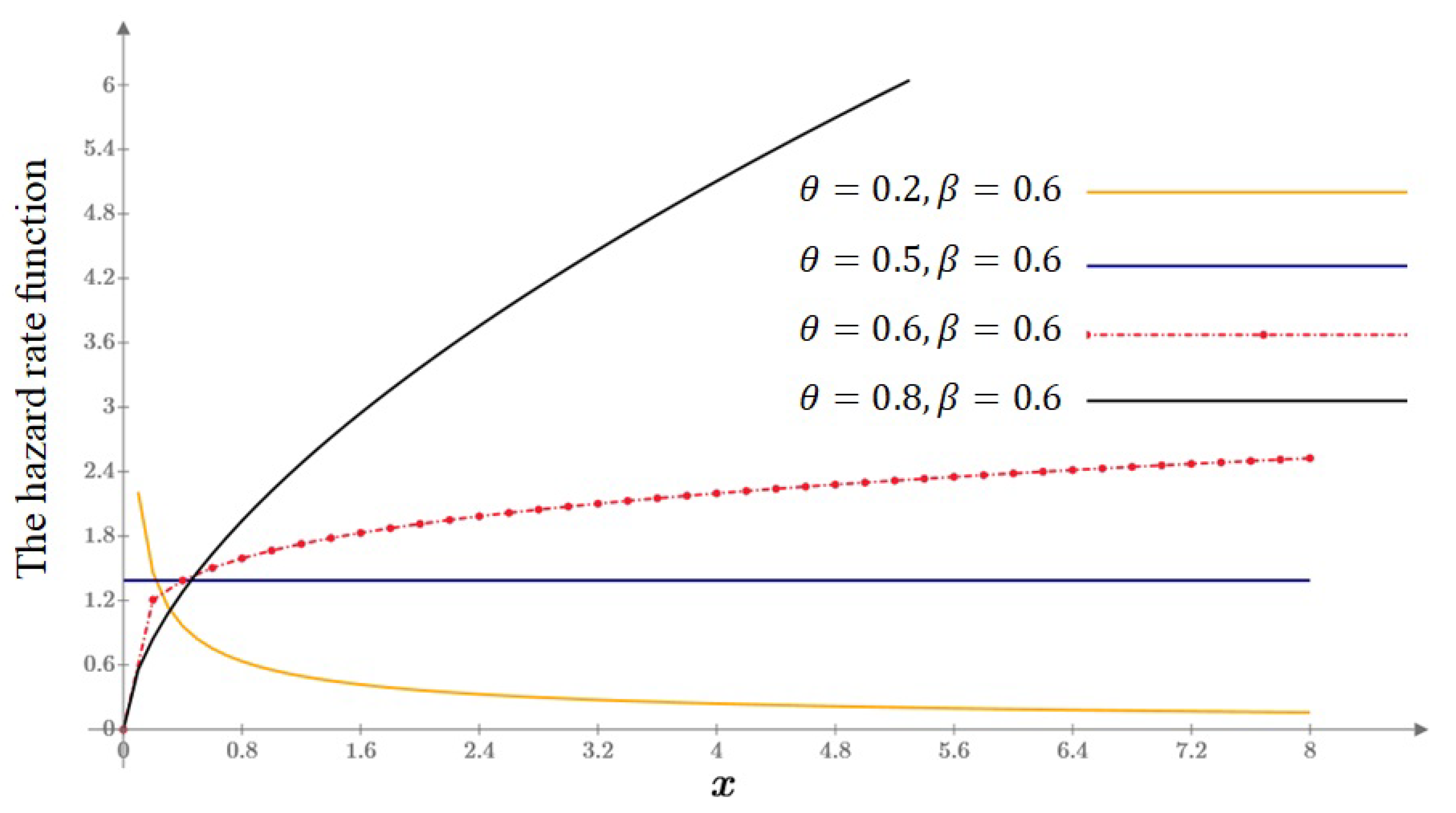
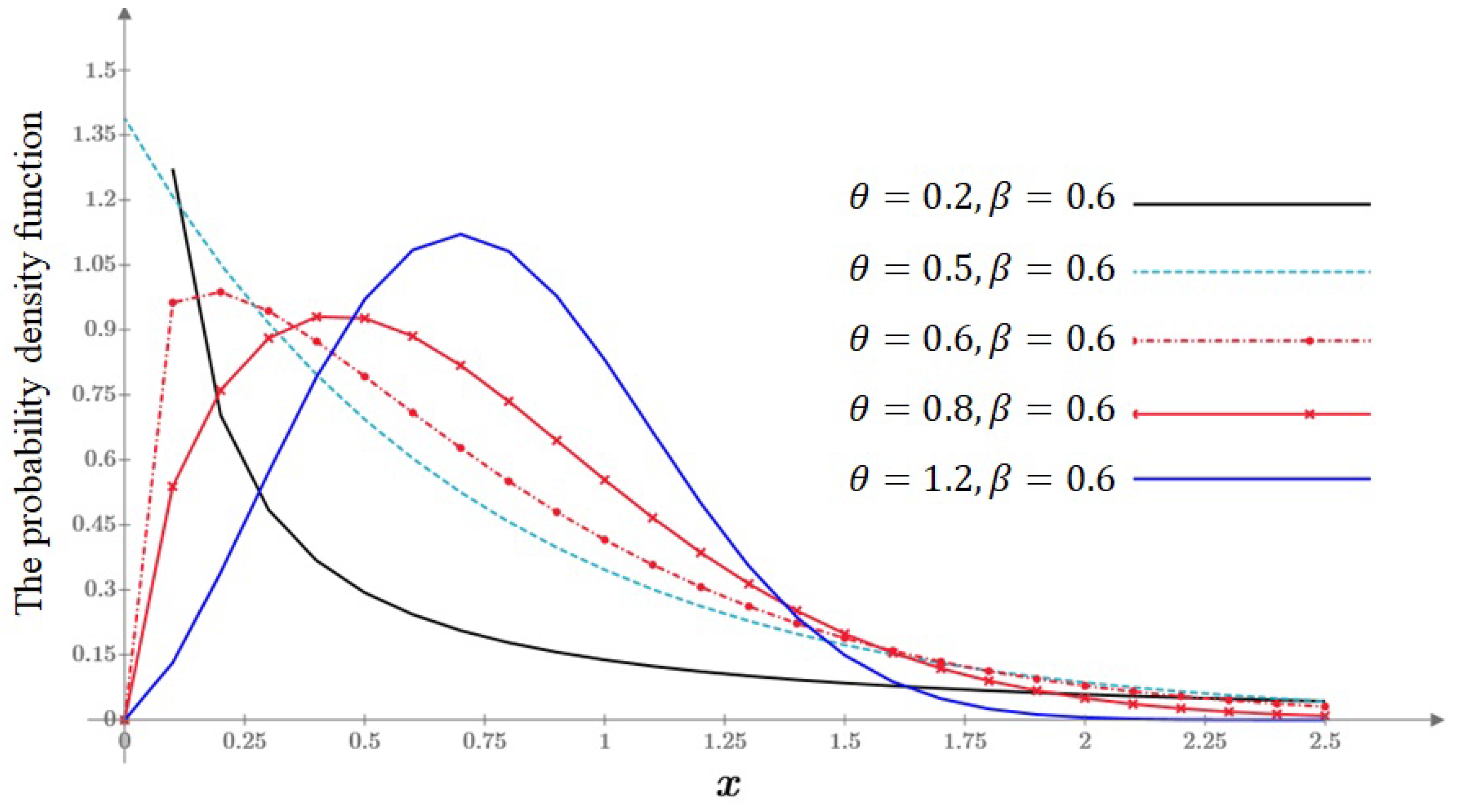
The HRF is increasing when $\theta >0.5$ and constant for $\theta =0.5$, while it is decreasing if $\theta <0.5$ for all x. The graphs for the PDF and HRF for different values of $\theta$ and $\beta$ are given as follows.

Based on Figure 1, the PR distribution is unimodal when $\theta >0.5$. Analysis of the PDF confirms that a distinct mode exists under this condition. The PR distribution has a significantly heavier right tail than many standard probability distributions.

The behavior of the hazard function depends on the value of $\theta$, as is evident from the hazard function in Equation (4) and illustrated in Figure 2.

The main objective of this study is to develop statistical inference procedures for the Power Rayleigh accelerated life model under the Type-I GHCS, with particular emphasis on the derivation of maximum-likelihood estimation (MLE), while the interval estimates are obtained using bootstrap resampling techniques and the observed Fisher information matrix. The Bayesian estimation of the model parameters is also investigated. Since the posterior distribution lacks a closed-form expression, Markov-chain Monte Carlo (MCMC) techniques are employed for inference.

The rest of the paper is organized as follows. The model formulation and the experimental step-stress PALT (SS-PALT) design are presented in Section 2. Section 3 introduces the methods of estimation: ML methods are used for point and interval estimation, bootstrap confidence intervals, and Bayesian estimation techniques. In Section 4, the performance of the proposed methods is assessed through Monte Carlo simulation studies, as well as analyses of real and simulated datasets. Lastly, Section 5 offers closing thoughts.

2. Modeling of SS-PALT

Let us say the units are assessed with an SS-PALT as part of a Type-I GHCS. Each test has a fixed duration of time (T) and two counting parameters ($\kappa$ and r), which denote the failure thresholds. The stress-change duration is selected so that the monitored $\tau$ under standard usage conditions is $\tau$, and at $\tau$, a stress-level rise is enforced. The test concludes after the $\kappa$-th failure. If $x_{\kappa }>T$, the experiment terminates at $\min (T,x_{\kappa })$; otherwise, it terminates at $x_{\kappa }$. The resulting Type-I GHCS dataset is denoted by $\mathit{x}=(x_1,\cdots ,x_J)$, where the first J failures are observed under normal operating conditions. However, after the system is subjected to accelerated stress conditions, the remaining ($m-J$) failures take place. The purpose of this deliberate increase in stress is to hasten the failure mechanism. Thus, it is possible to represent the observed Type-I GHCS data as $\mathit{x}=\{x_1<x_2<x_3<\cdots <x_J<\tau <x_{J+1}<\cdots <x_m\}$.

Let T represent the entire amount of time spent on the test. Next, the SS-PALT model can be depicted by $\mathit{y}=\{y_1<y_2<y_3<\cdots <y_J<\tau <y_{J+1}<\cdots <y_m\}$. Here, the acceleration factor ($\alpha$) produces an effective lifetime (y). This shows the total amount of time spent operating under both normal and accelerated stress scenarios. As a result, the SS-PALT scheme defines a test unit’s lifetime variable as follows:

$$Y=\left\{\begin{array}{ccc}X,\hfill & \mathrm{if}\hfill & X\le \tau ,\hfill \\ \tau +\left({\displaystyle \frac{X-\tau }{\alpha }}\right)\hfill & \mathrm{if}\hfill & X>\tau .\hfill \end{array}\right.$$

(5)

In this case, X denotes the lifespan under average conditions, while $\alpha$ denotes the acceleration factor (i.e., the average life ratio under normal usage compared to accelerated usage), with $\alpha >1$. The T parameter denotes the time to shift between different levels of applied stress. We consider the lifespans of the tested units to follow a PR ($\theta ,\beta$) distribution. Below are the PDF and CDF associated with the lifetime model given in Equation (5):

$$\begin{array}{ccc}\hfill F_Y\left(y\right)& =& \left\{\begin{array}{ccc}{F}_1\left(y\right)=1-e^{-{\displaystyle \frac{y^{2\theta }}{2{\beta }^2}}},\hfill & \mathrm{if}& y\le \tau ,\hfill \\ F_2\left(y\right)=1-e^{-{\displaystyle \frac{\left(\tau +\alpha {(y-\tau )}^{2\theta }\right)}{2{\beta }^2}}},\hfill & \mathrm{if}& y>\tau ,\hfill \end{array}\right.\hfill \\ \hfill f_Y\left(y\right)& =& \left\{\begin{array}{ccc}{f}_1\left(y\right)={\displaystyle \frac{\theta }{{\beta }^2}}{y}^{2\theta -1}{e}^{-{\displaystyle \frac{y^{2\theta }}{2{\beta }^2}}},\hfill & \mathrm{if}& y\le \tau ,\hfill \\ f_2\left(y\right)={\displaystyle \frac{\theta \alpha }{{\beta }^2}}{\left(\tau +\alpha (y-\tau )\right)}^{2\theta -1}{e}^{-{\displaystyle \frac{{\left(\tau +\alpha (y-\tau )\right)}^{2\theta }}{2{\beta }^2}}},\hfill & \mathrm{if}& y>\tau .\hfill \end{array}\right.\hfill \end{array}$$

The SF and HRF are

$$\begin{array}{ccc}\hfill S_Y\left(y\right)& =& \left\{\begin{array}{ccc}{S}_1\left(y\right)=e^{-{\displaystyle \frac{y^{2\theta }}{2{\beta }^2}}},\hfill & \mathrm{if}& y\le \tau ,\hfill \\ S_2\left(y\right)=e^{-{\displaystyle \frac{\left(\tau +\alpha {(y-\tau )}^{2\theta }\right)}{2{\beta }^2}}},\hfill & \mathrm{if}& y>\tau ,\hfill \end{array}\right.\hfill \\ \hfill h_Y\left(y\right)& =& \left\{\begin{array}{ccc}{h}_1\left(y\right)={\displaystyle \frac{\theta }{{\beta }^2}}{y}^{2\theta -1},\hfill & \mathrm{if}& y\le \tau ,\hfill \\ h_2\left(y\right)={\displaystyle \frac{\theta \alpha }{{\beta }^2}}{\left(\tau +\alpha (y-\tau )\right)}^{2\theta -1},\hfill & \mathrm{if}& y>\tau .\hfill \end{array}\right.\hfill \end{array}$$

The joint probability function of observed times $\mathit{y}=\{y_1<y_2<y_3<\cdots <y_J<\tau <y_{J+1}<\cdots <y_m\}$ is given by

$$f\left(\mathit{y}\right|\theta ,\beta ,\alpha )\propto {\displaystyle \prod _{i=1}^J}{f}_1\left(y_i\right){\displaystyle \prod _{i=J+1}^m}{f}_2\left(y_i\right){\left[S_2\left(y_m\right)\right]}^{n-m}$$

(6)

3. Methods of Estimation

This section presents the estimation procedures for the proposed model parameters and the acceleration factor. Specifically, MLE is employed for point and interval estimation, bootstrap methods are used to construct confidence intervals, and Bayesian inference is developed to obtain posterior estimates and credible intervals.

3.1. Frequentist Estimation

The likelihood function obtained from the observed accelerated Type-I GHCS ($\mathit{y}=(y_1<y_2<y_3<\cdots <y_J<\tau <y_{J+1}<\cdots <y_m)$) can be obtained by substituting Equations (2), (3), and (5) into Equation (6), yielding the following:

$$L(\theta ,\beta ,\alpha |\mathit{y})\propto e^{-{\displaystyle \frac{(n-m){(\tau +\alpha (y_m-\tau ))}^{2\theta }}{2{\beta }^2}}}{\displaystyle \prod _{i=1}^J}{\displaystyle \frac{\theta }{{\beta }^2}}{y}_i^{2\theta -1}{e}^{-{\displaystyle \frac{y_i^{2\theta }}{2{\beta }^2}}}{\displaystyle \prod _{i=J+1}^m}{\displaystyle \frac{\theta \alpha }{{\beta }^2}}{(\tau +\alpha (y_i-\tau ))}^{2\theta -1}{e}^{-{\displaystyle \frac{{(\tau +\alpha (y_i-\tau ))}^{2\theta }}{2{\beta }^2}}}.$$

(7)

The natural logarithm of $L(\theta ,\beta ,\alpha |\mathit{y})$ is expressed by

$$\begin{array}{ccc}\hfill \ell (\theta ,\beta ,\alpha |\mathit{y})& \propto & -{\displaystyle \frac{(n-m)}{2{\beta }^2}}{\left(\tau +\alpha (y_m-\tau )\right)}^{2\theta }+mlog\left({\displaystyle \frac{\theta }{{\beta }^2}}\right)+(2\theta -1){\displaystyle \sum _{i=1}^J}log\left(y_i\right)-{\displaystyle \frac{1}{2{\beta }^2}}{\displaystyle \sum _{i=1}^J}{y}_i^{2\theta }\hfill \\ & & +(m-J)log\left(\alpha \right)+(2\theta -1){\displaystyle \sum _{i=J+1}^m}log\left(\tau +\alpha (y_i-\tau )\right)-{\displaystyle \frac{1}{2{\beta }^2}}{\displaystyle \sum _{i=J+1}^m}{(\tau +\alpha (y_i-\tau ))}^{2\theta }.\hfill \end{array}$$

(8)

Equating the first partial derivatives of Equation (8) with respect to $\Theta =(\theta ,\beta ,\alpha )$ to zero yields the following system of equations:

$$\begin{array}{ccc}\hfill {\displaystyle \frac{\partial \ell (\theta ,\beta ,\alpha |\mathit{y})}{\partial \theta }}& =& {\displaystyle \frac{m}{\theta }}+2{\displaystyle \sum _{i=1}^J}log\left(y_i\right)+2{\displaystyle \sum _{i=J+1}^m}log\left(\tau +\alpha (y_i-\tau )\right)-{\displaystyle \frac{2}{{\beta }^2}}{\displaystyle \sum _{i=1}^J}{y}_i^{2\theta }log\left(y_i\right)\hfill \\ & & -{\displaystyle \frac{2}{2{\beta }^2}}{\displaystyle \sum _{i=J+1}^m}{\left(\tau +\alpha (y_i-\tau )\right)}^{2\theta }log(\tau +\alpha (y_i-\tau ))\hfill \\ & & +{\displaystyle \frac{n-m}{{\beta }^2}}{(\tau +\alpha (y_m-\tau ))}^{2\theta }log\left(\tau +\alpha (y_m-\tau )\right),\hfill \end{array}$$

(9)

$$\begin{array}{ccc}\hfill {\displaystyle \frac{\partial \ell (\theta ,\beta ,\alpha |\mathit{y})}{\partial \beta }}& =& {\displaystyle \frac{-2m}{\beta }}+{\displaystyle \frac{1}{{\beta }^3}}\left[2{\displaystyle \sum _{i=1}^J}{y}_i^{2\theta }+{\displaystyle \sum _{i=J+1}^m}{\left(\tau +\alpha (y_i-\tau )\right)}^{2\theta }+(m-n){\left(\tau +\alpha (y_m-\tau )\right)}^{2\theta }\right],\hfill \end{array}$$

(10)

$$\begin{array}{ccc}\hfill {\displaystyle \frac{\partial \ell (\theta ,\beta ,\alpha |\mathit{y})}{\partial \alpha }}& =& {\displaystyle \frac{m-J}{\alpha }}+(2\theta -1){\displaystyle \sum _{i=J+1}^m}{\displaystyle \frac{(y_i-\tau )}{\tau +\alpha (y_i-\tau )}}+{\displaystyle \frac{\theta }{{\beta }^2}}{\displaystyle \sum _{i=J+1}^m}\tau {(\tau +\alpha (y_i-\tau ))}^{2\theta -1}\hfill \\ & & -{\displaystyle \frac{\theta }{{\beta }^2}}{\displaystyle \sum _{i=J+1}^m}{y}_i{(\tau +\alpha (y_i-\tau ))}^{2\theta -1}+\left({\displaystyle \frac{n-m}{{\beta }^2}}\right)\theta (y_m-\tau ){(\tau +\alpha (y_m-\tau ))}^{2\theta -1}.\hfill \end{array}$$

(11)

By resolving the non-linear equation system found in Equations (9) through (11), the MLEs ($\widehat{\Theta }=(\widehat{\theta },\widehat{\beta },\widehat{\alpha })$) of the parameters ($\Theta$) are obtained. Numerical methods can be used to solve this system.

• Approximate interval estimation:

To construct the approximate confidence intervals, the Fisher information matrix is defined as the negative expected value of the second derivatives of the log-likelihood function ($\ell (\theta ,\beta ,\alpha |\mathit{y})$). Since deriving this expectation analytically is often difficult, the observed Fisher information matrix is commonly used as an approximation. The second-order partial derivatives of $\ell =\ell (\theta ,\beta ,\alpha |\mathit{y})$ with respect to $\Theta =(\theta ,\beta ,\alpha )$ are given as follows:

$$I\left(\widehat{\Theta }\right)={\left[\begin{array}{ccc}-E\left({\displaystyle \frac{{\partial }^2\ell }{\partial {\theta }^2}}\right)& -E\left({\displaystyle \frac{{\partial }^2\ell }{\partial \theta \partial \beta }}\right)& -E\left({\displaystyle \frac{{\partial }^2\ell }{\partial \theta \partial \alpha }}\right)\\ -E\left({\displaystyle \frac{{\partial }^2\ell }{\partial \beta \partial \theta }}\right)& -E\left({\displaystyle \frac{{\partial }^2\ell }{\partial {\beta }^2}}\right)& -E\left({\displaystyle \frac{{\partial }^2\ell }{\partial \beta \partial \alpha }}\right)\\ -E\left({\displaystyle \frac{{\partial }^2\ell }{\partial \alpha \partial \theta }}\right)& -E\left({\displaystyle \frac{{\partial }^2\ell }{\partial \alpha \partial \beta }}\right)& -E\left({\displaystyle \frac{{\partial }^2\ell }{\partial {\alpha }^2}}\right)\end{array}\right]}_{(\theta ,\beta ,\alpha )\to (\widehat{\theta },\widehat{\beta },\widehat{\alpha })},$$

(12)

where the second partial derivatives are given as follows:

$$\begin{array}{ccc}\hfill {\displaystyle \frac{{\partial }^2\ell }{\partial {\theta }^2}}& =& {\displaystyle \frac{m}{{\theta }^2}}-{\displaystyle \frac{4}{{\beta }^2}}{\displaystyle \sum _{i=1}^J}{y}_i^{2\theta }log{\left(y_i\right)}^2-{\displaystyle \frac{2}{{\beta }^2}}{\displaystyle \sum _{i=J+1}^m}{(\tau +\alpha (y_i-\tau ))}^{2\theta }log{(\tau +\alpha (y_i-\tau ))}^2\hfill \\ & & +{\displaystyle \frac{2}{{\beta }^2}}(n-m){(\tau +\alpha (y_m-\tau ))}^{2\theta }log{(\tau +\alpha (y_m-\tau ))}^2,\hfill \\ \hfill {\displaystyle \frac{{\partial }^2\ell }{\partial \theta \partial \beta }}& =& {\displaystyle \frac{4}{{\beta }^3}}{\displaystyle \sum _{i=1}^J}{y}_i^{2\theta }log\left(y_i\right)+{\displaystyle \frac{2}{{\beta }^3}}{\displaystyle \sum _{i=J+1}^m}{(\tau +\alpha (y_i-\tau ))}^{2\theta }log(\tau +\alpha (y_i-\tau ))\hfill \\ & & -{\displaystyle \frac{2}{{\beta }^3}}(n-m){(\tau +\alpha (y_m-\tau ))}^{2\theta }log(\tau +\alpha (y_m-\tau )),\hfill \\ \hfill {\displaystyle \frac{{\partial }^2\ell }{\partial \theta \partial \alpha }}& =& 2{\displaystyle \sum _{i=J+1}^m}{\displaystyle \frac{y_i-\tau }{\tau +\alpha (y_i-\tau )}}+{\displaystyle \frac{1}{{\beta }^2}}(n-m)(y_m-\tau ){(\tau +\alpha (y_m-\tau ))}^{2\theta -1}\hfill \\ & & -{\displaystyle \frac{2}{2{\beta }^2}}{\displaystyle \sum _{i=1+J}^m}{(\tau +\alpha (y_i-\tau ))}^{2\theta -1}(y_i-T)\left[1+2\theta log(\tau +\alpha (y_i-\tau ))\right]\hfill \\ & & +{\displaystyle \frac{2\theta }{{\beta }^2}}(n-m)(y_m-\tau ){(\tau +\alpha (y_m-\tau ))}^{2\theta -1}log(\tau +\alpha (y_m-\tau )),\hfill \\ \hfill {\displaystyle \frac{{\partial }^2\ell }{\partial {\beta }^2}}& =& {\displaystyle \frac{2m}{{\beta }^2}}-{\displaystyle \frac{6}{{\beta }^4}}{\displaystyle \sum _{i=1}^J}{y}_i^{2\theta }-{\displaystyle \frac{3}{{\beta }^4}}{\displaystyle \sum _{i=1+J}^m}{(\tau +\alpha (y_i-\tau ))}^{2\theta }+{\displaystyle \frac{3}{{\beta }^4}}(n-m){(\tau +\alpha (y_m-\tau ))}^{2\theta },\hfill \\ \hfill {\displaystyle \frac{{\partial }^2\ell }{\partial \beta \partial \alpha }}& =& {\displaystyle \frac{2\theta }{{\beta }^3}}{\displaystyle \sum _{i=1+J}^m}{(\tau +\alpha (y_i-\tau ))}^{2\theta -1}(y_i-\tau )-{\displaystyle \frac{2\theta }{{\beta }^3}}(n-m)(y_m-\tau ){(\tau +\alpha (y_m-\tau ))}^{2\theta -1},\hfill \\ \hfill {\displaystyle \frac{{\partial }^2\ell }{\partial {\alpha }^2}}& =& -{\displaystyle \frac{m-J}{{\alpha }^2}}-(2\theta -1){\displaystyle \sum _{i=J+1}^m}{\displaystyle \frac{{(y_i-\tau )}^2}{{(\tau +\alpha (y_i-\tau ))}^2}}-{\displaystyle \frac{\theta (2\theta -1)}{{\beta }^2}}{\displaystyle \sum _{i=J+1}^m}{(y_i-\tau )}^2{(\tau +\alpha (y_i-\tau ))}^{2\theta -2}\hfill \\ & & +{\displaystyle \frac{1}{{\beta }^2}}(n-m)\theta (2\theta -1){(y_m-\tau )}^2{(\tau +\alpha (y_m-\tau ))}^{2\theta -2}.\hfill \end{array}$$

The $\widehat{\Theta }$ is roughly distributed as a multivariate normal vector with mean ($\Theta$) and variance-covariance matrix ($I^{-1}\left(\widehat{\Theta }\right)$) based on the asymptotic features of MLEs:

$$\widehat{\Theta }\sim N\left(\Theta ,I^{-1}(\widehat{\Theta })\right).$$

The approximate $100(1-\nu )\%$ interval estimates of $\Theta =(\theta ,\beta ,\alpha )$ are

$$\widehat{\theta }\pm z_{\nu /2}\sqrt{var(\widehat{\theta })},\widehat{\beta }\pm z_{\nu /2}\sqrt{var(\widehat{\beta })}\mathrm{and}\widehat{\alpha }\pm z_{\nu /2}\sqrt{(var(\widehat{\alpha })}$$

(13)

3.2. Bootstrap Method

Following the framework established by Davison and Hinkley [20], this study utilizes the parametric percentile bootstrap technique as a robust mechanism for interval estimation. This technique, further elaborated upon in the seminal work of Efron and Tibshirani [21], is implemented here to construct confidence intervals and rigorously evaluate the variance and bias of the proposed estimators (Algorithm 1).

Algorithm 1: Percentile Bootstrap

1. The original failure data vector $\mathit{y}=(y_1<y_2<y_3,\cdots ,y_J<\tau <y_{J+1}<\cdots <y_m)$ is derived utilizing pre-specified numbers $\kappa ,r$, the stress-change time ($\tau$), and an empirical dataset of size n. 2. Calculate the first MLEs from the original dataset $\mathit{y}$, represented as $\widehat{\Theta }=(\widehat{\theta },\widehat{\beta },\widehat{\alpha })$. 3. Set the bootstrap iteration counter’s initial value to $i=1$. 4. Using the initial censoring constraints, generate a Type-I GHC random sample from the provided distribution $(n,\kappa ,r,\tau )$ and the estimated parameter $\widehat{\Theta }$. 5. To create the accelerated bootstrap sample ${\mathit{y}}^{*}=(y_1^{*},y_2^{*},\cdots ,y_J^{*},\tau ,y_{J+1}^{*},\cdots ,y_m^{*}$, apply the PALT transformation, Equation (5), to all simulated observations that are longer than the stress-change time. 6. Based on the sample ${\mathit{y}}^{*}$, calculate the bootstrap MLEs ${\widehat{\Theta }}^{*}=({\widehat{\theta }}^{*},{\widehat{\beta }}^{*},{\widehat{\alpha }}^{*})$. 7. Increase the counter $i=i+1$. 8. To create a series of bootstrap estimates, repeat Steps 4 through 7, N times $${\widehat{\Theta }}^{*}={\displaystyle \frac{1}{N}}{\displaystyle \sum _{i=1}^N}{\widehat{\Theta }}^{{*}^{\left(i\right)}},$$ (14) 9. The approximate $100(1-\nu )\%$ confidence interval for parameters $\widehat{\Theta }=(\widehat{\theta },\widehat{\beta },\widehat{\alpha })$ and $i=1,\cdots ,N$, are given, respectively, by $$\left({\widehat{\theta }}^{*\left[N\right(\nu /2\left)\right]},{\widehat{\theta }}^{*\left[N\right(1-\nu /2\left)\right]}\right),\left({\widehat{\beta }}^{*\left[N\right(\nu /2\left)\right]},{\widehat{\beta }}^{*\left[N\right(1-\nu /2\left)\right]}\right),\mathrm{and}\left({\widehat{\alpha }}^{*\left[N\right(\nu /2\left)\right]},{\widehat{\alpha }}^{*\left[N\right(1-\nu /2\left)\right]}\right).$$

3.3. Bayesian Estimation

One of the favored techniques for evaluating a variety of statistical models is the Bayesian method. Thus, based on Type-I GHC, Bayesian estimates (BE) and their related credible intervals for the unknown parameters ($\Theta =(\theta ,\beta ,\alpha )$) of the PR distribution are produced in this section. Both the loss function and the choice of distribution have an impact on Bayesian estimation. For this reason, the square error (SE) loss function is taken into consideration for the symmetric loss function. The posterior mean of the parameters is the BE under the SE loss function. Independent gamma priors are assigned to $\theta$ and $\beta$. Moreover, gamma priors provide considerable flexibility and allow prior information to be incorporated smoothly into the posterior inference. The independent gamma priors provided by

$${\pi }_1\left(\theta \right)\propto {\theta }^{a-1}{e}^{-b\theta },{\pi }_2\left(\beta \right)\propto {\beta }^{c-1}{e}^{-d\beta },$$

(15)

where $a,b,c$, and d are known hyperparameters, the acceleration factor $\alpha$ has a noninformative prior (NIP).

$${\pi }_3\left(\alpha \right)\propto 1/\alpha$$

(16)

In the limiting case where all hyperparameters are set to zero, in the case of an NIP, the joint prior for the parameter vector expressed as $\Theta =(\theta ,\beta ,\alpha )$ is given as follows:

$$\pi (\theta ,\beta ,\alpha )\propto {\theta }^{a-1}{\beta }^{c-1}{\alpha }^{-1}{e}^{-(b\theta +c\beta )},\theta ,\beta ,\alpha >0.$$

(17)

The joint posterior density of the parameters ($\Theta =(\theta ,\beta ,\alpha )$) is obtained by combining the likelihood and the prior density of Equation (17) as follows:

$${\pi }^{*}(\theta ,\beta ,\alpha |\mathit{y})\propto \pi (\theta ,\beta ,\alpha )L(\theta ,\beta ,\alpha |\mathit{y}).$$

(18)

Then, the theoretical formulation of the BE for the parameters ($\Theta =(\theta ,\beta ,\alpha )$) under the SE loss function is calculated as follows:

$${\widehat{\Theta }}_{i_{SE}}={\int }_{\Theta }{\Theta }_i{\pi }^{*}(\Theta )d{\Theta }_i,i=1,2,3.$$

(19)

The posterior expectations are analytically intractable and, therefore, are approximated using different methods, such as Lindley’s approach and, more commonly, MCMC techniques. These techniques rely on algorithms like significance sampling, the Metropolis–Hastings algorithm (MH) within the Gibbs algorithm, and Gibbs sampling to generate samples and construct an empirical posterior distribution.

The significance of MCMC methodology is emphasized by the extensive corpus of recent statistical literature. Its usefulness stems from its capacity to produce interval estimates, as well as point estimates, using the final simulated empirical distribution. Iteratively sampling from the posterior distributions of the model is how MCMC operates. Gibbs sampling and the MH-within-Gibbs sampler are two of the most significant methods in this category; for further information, see the works by Robert and Casella [22] and Ahmed and Ismail [23].

Given the data, we can calculate the joint posterior density of $\Theta =(\theta ,\beta ,\alpha )$ as follows:

$$\begin{array}{ccc}\hfill {\pi }^{*}(\theta ,\beta ,\alpha |\mathit{y})& \propto & {\theta }^{a+m-1}{\beta }^{c-2m-1}{\alpha }^{m-J-1}{e}^{-(b\theta +c\beta )}exp\left\{-{\displaystyle \frac{1}{2{\beta }^2}}\left[(n-m){(\tau +\alpha (y_m-\tau ))}^{2\theta }\right.\right.\hfill \\ & & \left.\left.+{\displaystyle \sum _{i=1}^J}{y}_i^{2\theta }+{\displaystyle \sum _{i=J+1}^m}{(\tau +\alpha (y_i-\tau ))}^{2\theta }\right]\right\}{\displaystyle \prod _{i=1}^J}{y}_i^{2\theta -1}{\displaystyle \prod _{i=J+1}^m}{[\tau +\alpha (y_i-\tau )]}^{2\theta -1}.\hfill \end{array}$$

(20)

Hence, the definition of the conditional posterior densities is

$$\begin{array}{ccc}\hfill {\pi }_{\theta }^{*}\left(\theta \right|\beta ,\alpha ,\mathit{y})& \propto & {\theta }^{a+m-1}{e}^{-b\theta -{\displaystyle \frac{1}{2{\beta }^2}}\left[(n-m){(\tau +\alpha (y_m-\tau ))}^{2\theta }+{\sum }_{i=1}^J{y}_i^{2\theta }+{\sum }_{i=J+1}^m{(\tau +\alpha (y_i-\tau ))}^{2\theta }\right]}\times \hfill \\ & & {\displaystyle \prod _{i=1}^J}{y}_i^{2\theta -1}{\displaystyle \prod _{i=J+1}^m}{[\tau +\alpha (y_i-\tau )]}^{2\theta -1}.\hfill \end{array}$$

(21)

$$\begin{array}{ccc}\hfill {\pi }_{\beta }^{*}\left(\beta \right|\theta ,\alpha ,\mathit{y})& \propto & {\beta }^{c-2m-1}{e}^{-c\beta -{\displaystyle \frac{1}{2{\beta }^2}}\left[(n-m){(\tau +\alpha (y_m-\tau ))}^{2\theta }+{\sum }_{i=1}^J{y}_i^{2\theta }+{\sum }_{i=J+1}^m{(\tau +\alpha (y_i-\tau ))}^{2\theta }\right]}.\hfill \end{array}$$

(22)

and

$${\pi }_{\alpha }^{*}\left(\alpha \right|\theta ,\beta ,\mathit{y})\propto {\alpha }^{m-J-1}{e}^{-{\displaystyle \frac{1}{2{\beta }^2}}\left[(n-m){(\tau +\alpha (y_m-\tau ))}^{2\theta }+{\sum }_{i=J+1}^m{(\tau +\alpha (y_i-\tau ))}^{2\theta }\right]}{\displaystyle \prod _{i=J+1}^m}{[\tau +\alpha (y_i-\tau )]}^{2\theta -1}.$$

(23)

The distributions in Equations (21)–(23) cannot be sampled directly using standard methods. Consequently, a normal proposal distribution MH step is used, since the conditional posterior distributions exhibit approximately normal behavior. This procedure enables the estimation of the posterior means and marginal posterior distributions, which are essential components of Bayesian inference. The MCMC (MH) algorithm used to generate posterior samples of $\theta ,\beta$, and $\alpha$ is outlined as follows (Algorithm 2):

Algorithm 2: MCMC  method

1. Begin with initial guess values, ${\Theta }^{\left(0\right)}=(\widehat{\theta },\widehat{\beta },\widehat{\alpha })$. 2. Set up the iterative loop $i=1$. 3. For each parameter in $\Theta$, a candidate value ${\theta }^{*}$ is generated from the conditional posterior ${\pi }_{\theta }^{*}\left(\theta \right|\beta ,\alpha ,y)$ using the MH algorithm with a normal proposal distribution $N\left({\theta }^{(i-1)},var\left(\widehat{\theta }\right)\right)$, where $var\left(\widehat{\theta }\right)$ is the variance of $\Theta$ in the variance-covariance matrix $I^{-1}\left(\widehat{\Theta }\right)$, based on the asymptotic features of MLEs. (a) The acceptance probability is computed using the ratio of posterior densities: $$q\left(\theta \right)=\min \left[1,{\displaystyle \frac{{\pi }_{\theta }\left({\theta }^{*}\right|{\beta }^{(i-1)},{\alpha }^{(i-1)},w)}{{\pi }_{\theta }\left({\theta }^{(i-1)}\right|{\beta }^{(i-1)},{\alpha }^{(i-1)},w)}}\right].$$ (b) Candidates are accepted or rejected based on a uniform random variable, such as: $U\sim \mathrm{Uniform}$. If $U\le q\left(\theta \right)$, set ${\theta }^{\left(i\right)}={\theta }^{*}$; otherwise, set ${\theta }^{\left(i\right)}={\theta }^{(i-1)}$. 4. Repeat Step (3) for parameters $\beta$ and $\alpha$. 5. Set $i=i+1$ 6. Repeat steps 3–5, N times to get ${\Theta }^{\left(1\right)},{\Theta }^{\left(2\right)},\cdots ,{\Theta }^{\left(N\right)}$, where ${\Theta }^{\left(i\right)}=\left({\theta }^{\left(i\right)},{\beta }^{\left(i\right)},{\alpha }^{\left(i\right)}\right)$ and $i=1,2,\cdots ,N$ 7. After completing iterations, the app discards the first samples (burn-in) and calculates the Bayesian Mean Estimate, which is given by: $$\widehat{\Theta }={\displaystyle \frac{1}{N-M}}{\displaystyle \sum _{i=1}^{N-M}}{\widehat{\Theta }}^{\left(i\right)},\Theta =(\theta ,\beta ,\alpha )$$ (24) 8. Order ${\Theta }^{(M+1)},{\Theta }^{(M+2)},\cdots ,{\Theta }^{\left(N\right)}$ as ${\Theta }_{\left(1\right)}<{\Theta }_{\left(2\right)}<\cdots <{\Theta }_{(N-M)}$,The approximate $100(1-\nu )\%$ credible interval for parameters $\Theta =(\theta ,\beta ,\alpha )$, are given, respectively, by $$\left({\widehat{\Theta }}^{\left[\right(N-M\left)\right(\nu /2\left)\right]},{\widehat{\Theta }}^{\left[\right(N-M\left)\right(1-\nu /2\left)\right]}\right).$$ (25)

4. Numerical Studies

To assess the reliability of the proposed estimation methods, their performance is evaluated using both Monte Carlo simulation and real data analysis. The simulation study examines the empirical bias and mean squared error (MSE) under different sample sizes and censoring schemes, providing practical evidence of the estimators’ finite-sample performance. The real data application further demonstrates the applicability and effectiveness of the proposed methods in practical settings. These numerical results indicate satisfactory empirical performance.

4.1. Applications

Application 1.

The breaking stress measurements for 50 mm carbon fibers are discussed by Nicholas and Padgett [24]. These data were notably employed by Cordeiro and Lemonte [25] to illustrate the flexibility of the four-parameter BBS model over the classic two-parameter Birnbaum–Saunders distribution. An initial analysis reveals that the distribution of these measurements is unimodal and roughly symmetric, with the data set as follows: 12.2, 23.56, 23.74, 25.87, 31.98, 37.0, 41.35, 47.38, 55.46, 58.36, 63.47, 68.46, 74.47, 78.26, 81.43, 84, 92, 94, 110, 112, 119, 127, 130, 133, 140, 146, 155, 159, 173, 179, 194, 195, 209, 249, 281, 319, 339, 432, 469, 519, 633, 725, 817, 1776.

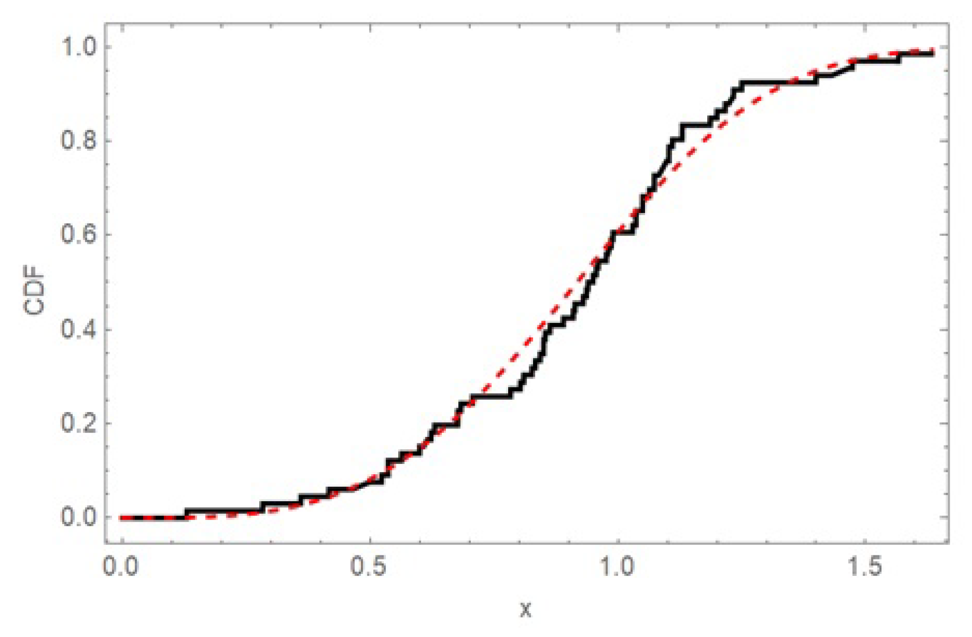
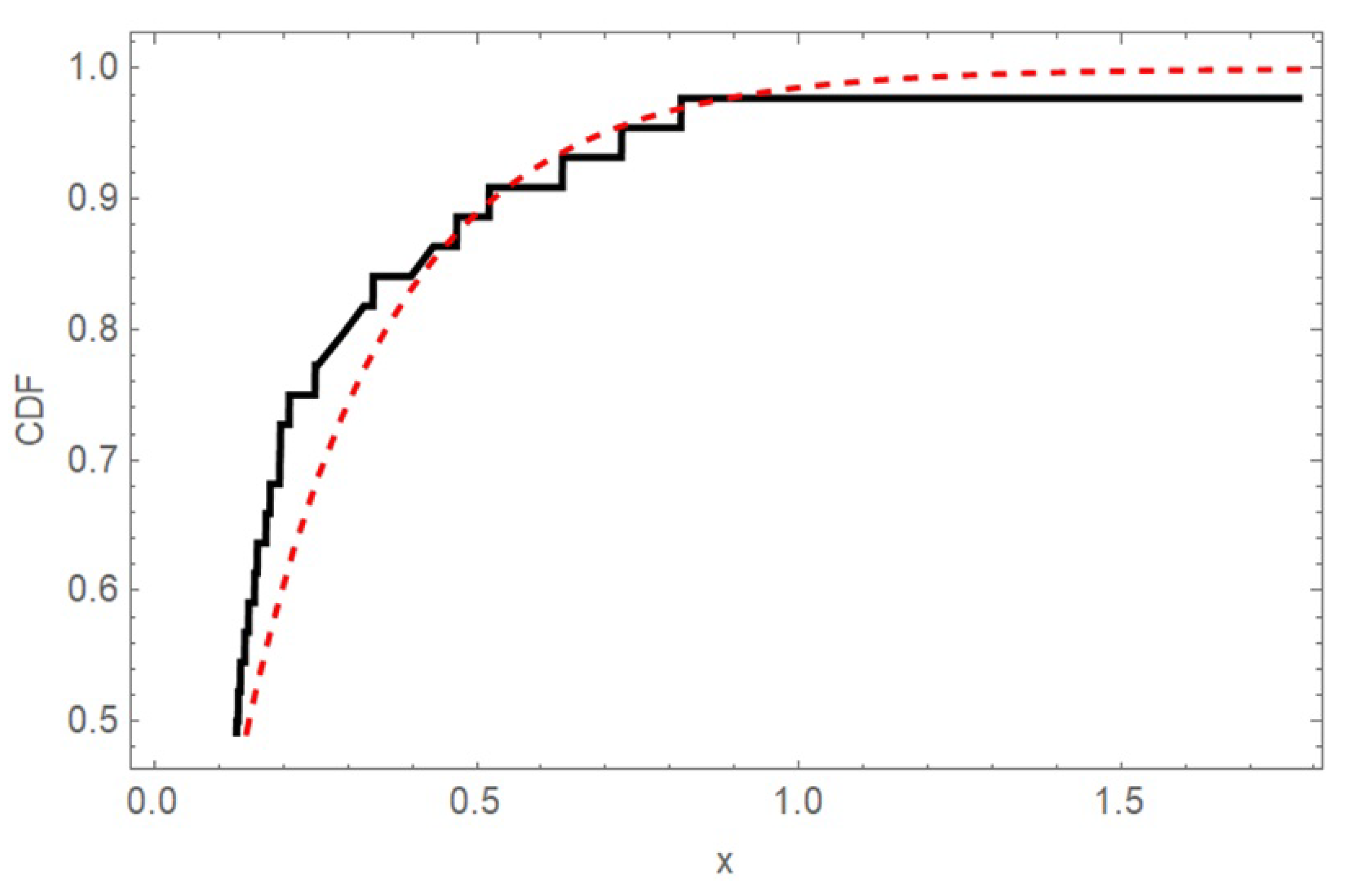
The appropriateness of the Power Rayleigh distribution with the $\theta ,\beta$, and $\alpha$ parameters was confirmed via K-S testing and visual inspection of the CDF in Figure 3. Transformation (data/1000) yielded a K-S distance of 0.1307 and p-value = 0.4399, demonstrating a satisfactory fit to real data 1.

The procedure for an accelerated Type-I GHCS can be characterized as follows: 0.0121, 0.0235, 0.02373, 0.02587, 0.0319, 0.037, 0.0413, 0.04738, 0.0554, 0.058, 0.0634, 0.0684, 0.0744, 0.0782, 0.0814, 0.084, 0.092, 0.094, 0.11, 0.112, 0.1190, 0.127, 0.13, 0.133, 0.14, 0.146, 0.155, 0.159, 0.17300, 0.179, 0.194, 0.195, 0.209, 0.249.

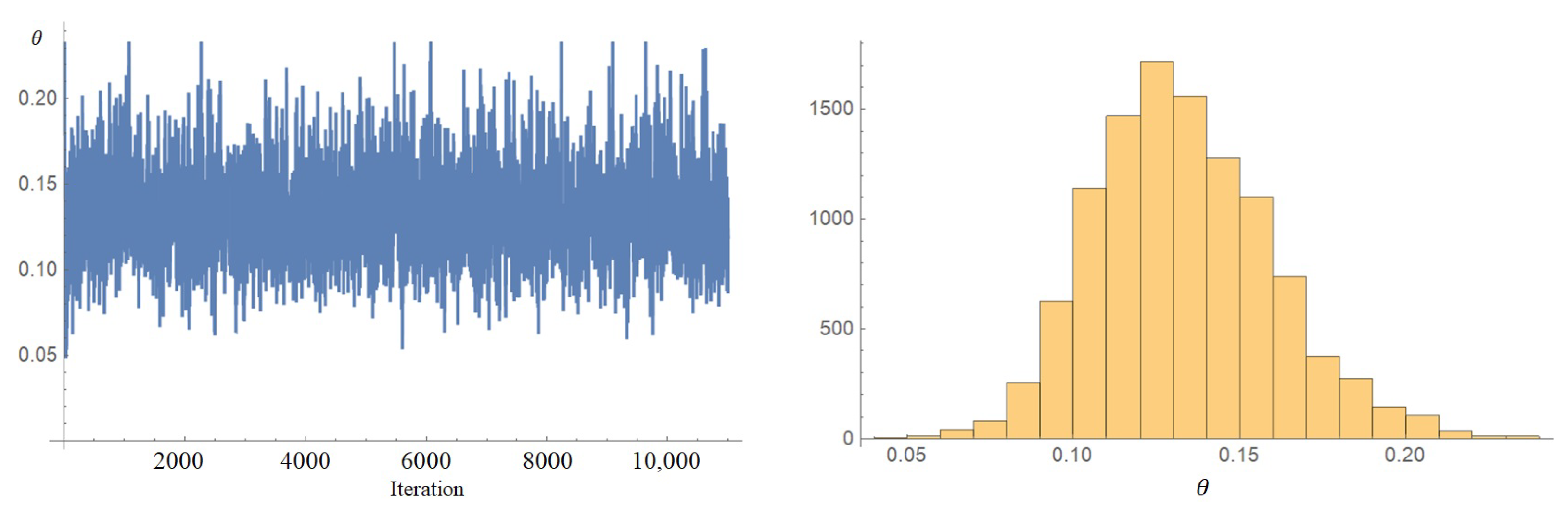
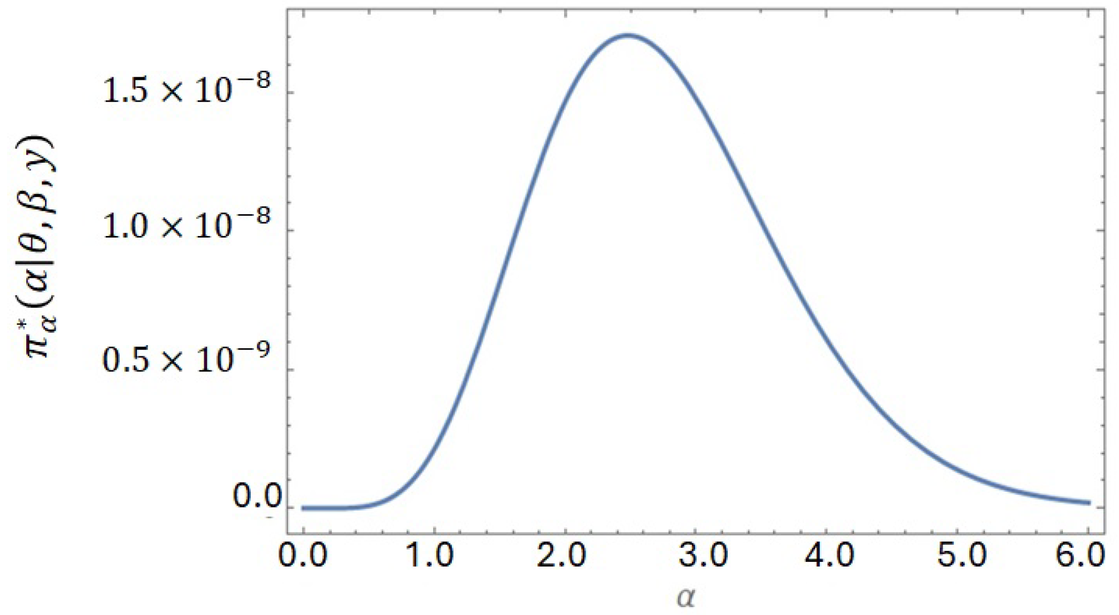
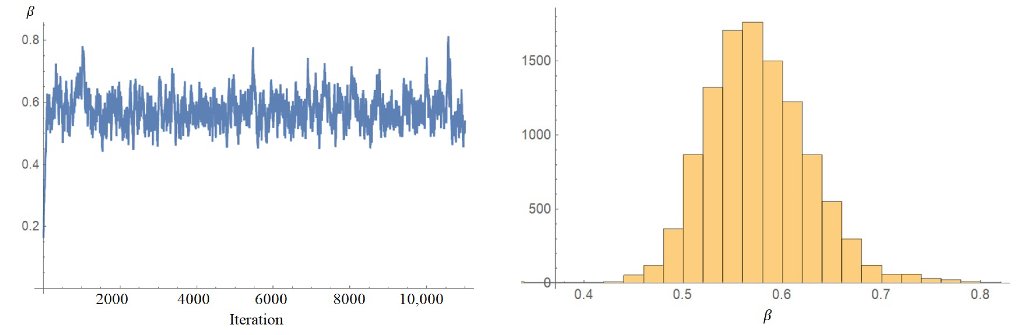
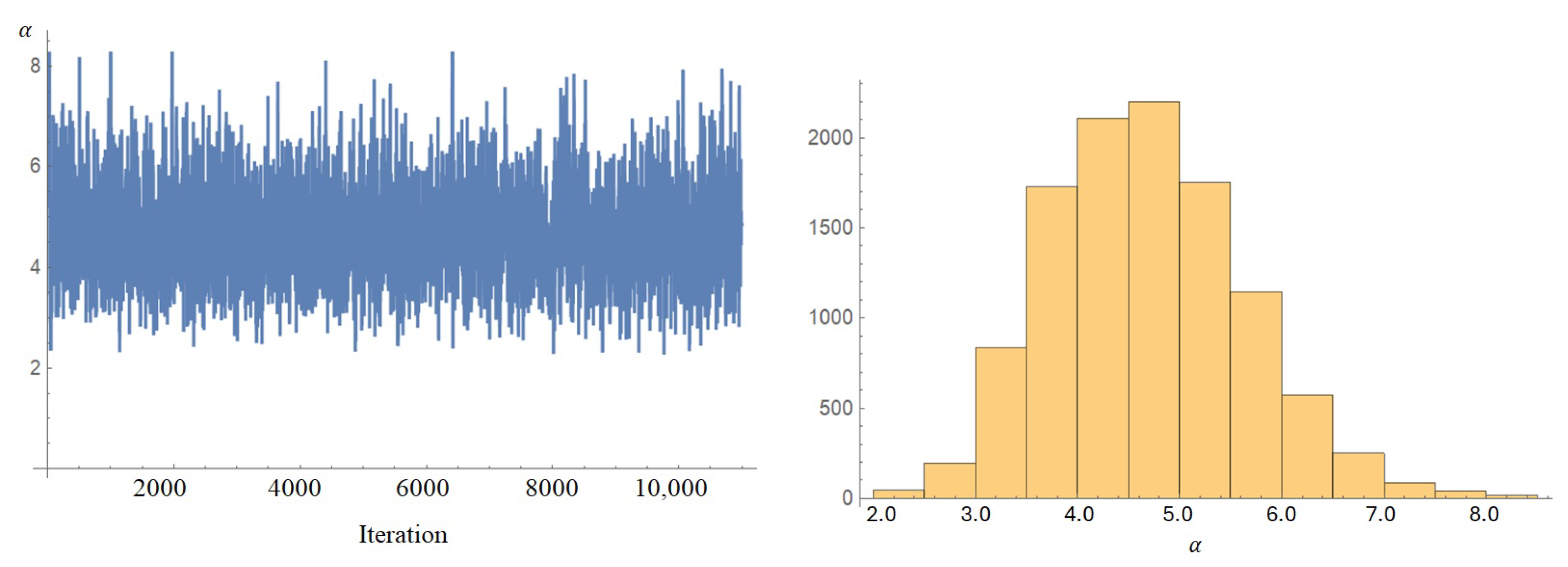
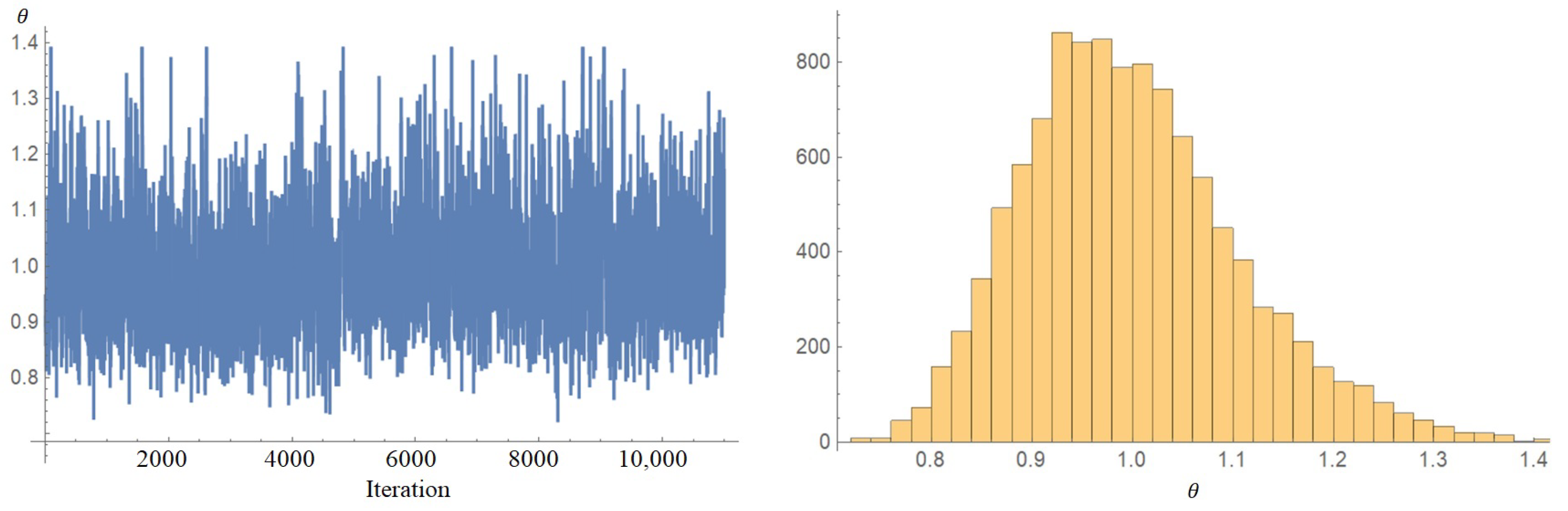
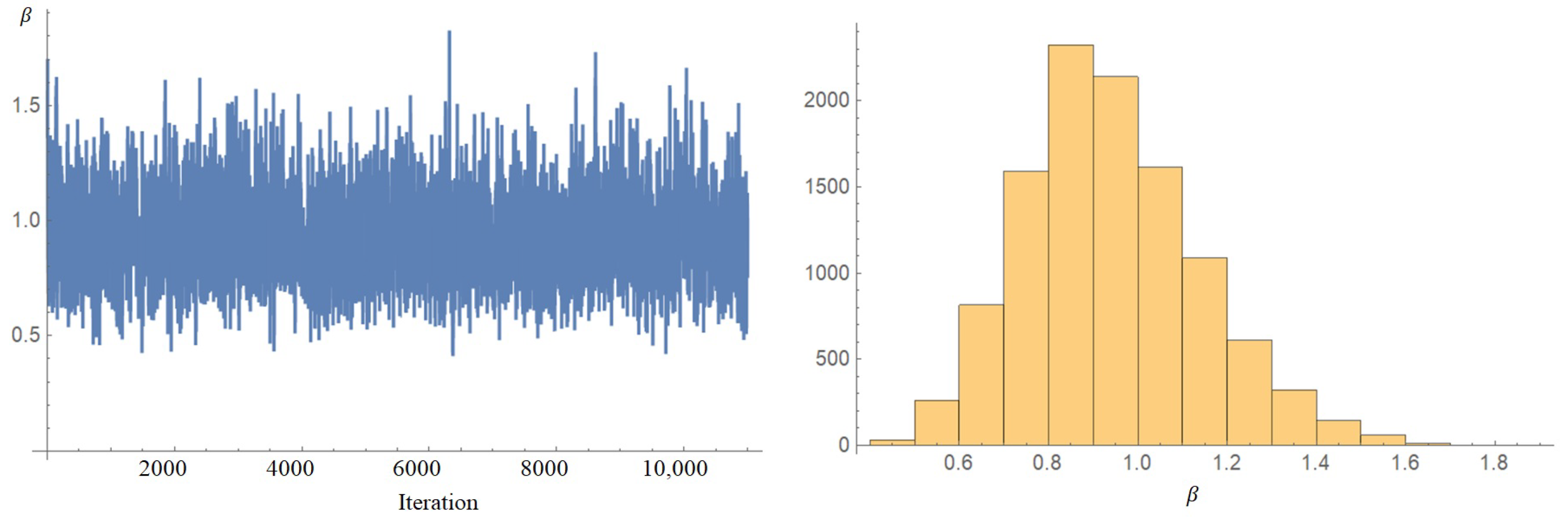
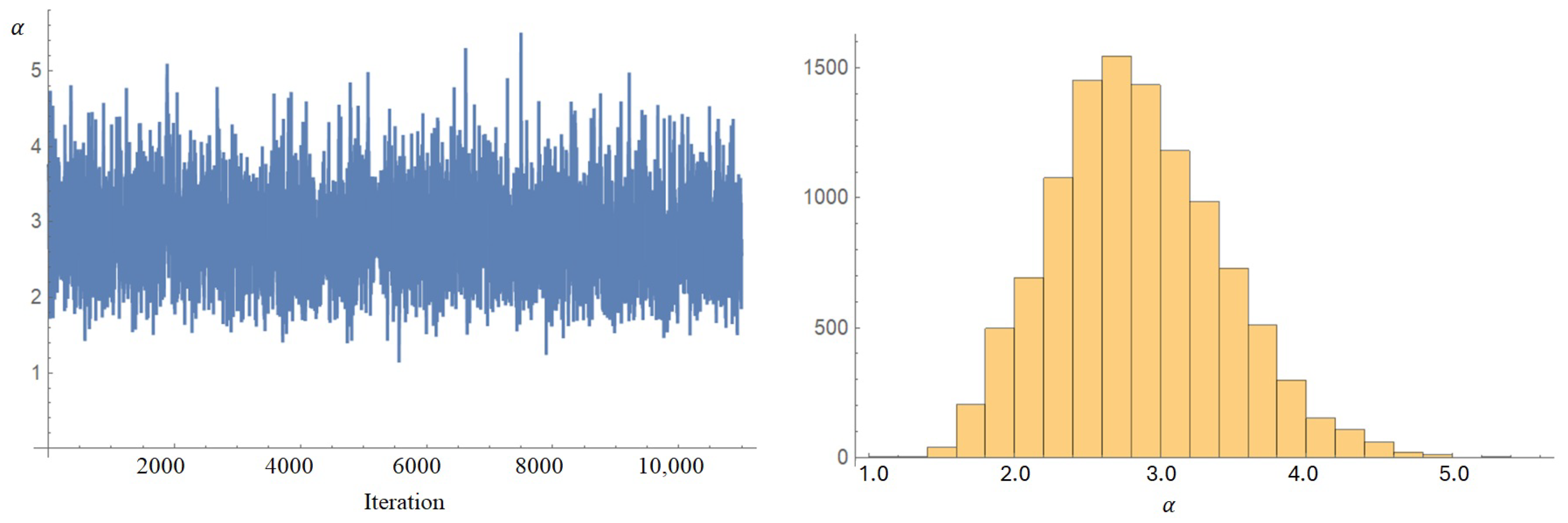
For application, an accelerated Type-I GHC sample was generated ($n=44$, $k=20$, $r=25$, $\tau =0.25$, and $T=0.3$), resulting in $J=34$ and $m=40$ failures. Parameter estimation was performed via MLE and Bayesian MCMC methods (11,000 samples, 1000 burn-ins). NIPs with hyperparameters of 0.0001 were utilized (see

Table 1. Point estimates for real data 1.

Parameter	MLE	MCMC	Boot-p
$\theta$	0.1472292	0.13321	0.14002
$\beta$	0.61591072	0.5741	0.5963
$\alpha$	5.02120951	5.00404	5.1271

and

Table 2. 95% confidence interval for real data 1.

Parameter	ACI	MCMC	Boot-p
$\theta$	(0.1132, 0.1813)	(0.1201, 0.1742)	(0.1103, 0.1811)
$\beta$	(0.500, 0.7318)	(0.5501, 0.7015)	(0.5001, 0.7105)
$\alpha$	(2.852, 7.1890)	(3.7852, 6.2015)	(3.9901, 6.7416)

). The posterior density plotted in Figure 4, Figure 5 and Figure 6 verifies the convergence and reliability of the MCMC algorithm.

The trace plots showed stable behavior, with no apparent systematic trends, and the posterior histograms exhibited well-defined unimodal distributions. Together with the reported acceptance rates, these graphical diagnostics provided evidence of satisfactory mixing and convergence of the MCMC chains, supporting the reliability of the Bayesian inference presented in this study.

Application 2.

The dataset from [26] consists of survival times (in months) for 44 patients treated for head-and-neck cancer with concurrent radiotherapy and chemotherapy, with the data set as follows: 0.39, 0.85, 1.08, 1.25, 1.47, 1.57, 1.61, 1.61, 1.69, 1.80, 1.84, 1.87, 1.89, 2.03, 2.03, 2.05, 2.12, 2.35, 2.41, 2.43, 2.48, 2.50, 2.53, 2.55, 2.55, 2.56, 2.59, 2.67, 2.73, 2.74, 2.79, 2.81, 2.82, 2.85, 2.87, 2.88, 2.93, 2.95, 2.96, 2.97, 3.09, 3.11, 3.11, 3.15, 3.15, 3.19, 3.22, 3.22, 3.27, 3.28, 3.31, 3.31, 3.33, 3.39, 3.39, 3.56, 3.60, 3.65, 3.68, 3.70, 3.75, 4.20, 4.38, 4.42, 4.70, 4.90.

The appropriateness of the Power Rayleigh distribution with $\theta ,\beta$, and $\alpha$ parameters was confirmed via K-S testing and visual inspection of the CDF in Figure 7.

Transformation (data/3) yielded a K-S distance of 0.0823 and p-value = 0.7627, demonstrating a satisfactory fit to the data. The procedure for an accelerated Type-I GHCS can be characterized as follows: 0.13, 0.28, 0.36, 0.41666, 0.49, 0.5233, 0.536, 0.536, 0.5633, 0.6, 0.6133, 0.6233, 0.6299, 0.6766, 0.676, 0.6833, 0.70666, 0.7833, 0.8033, 0.81, 0.8266, 0.8333, 0.8433, 0.84999, 0.8499.

For the application, an accelerated Type-I GHC sample was generated ($n=66$, $k=25$, $r=25$, $\tau =0.6$, and $T=0.75$), resulting in $J=18$ and $m=50$ failures. Parameter estimation was performed via MLE and Bayesian MCMC methods (11,000 samples and 1000 burn-ins). Non-informative priors with hyperparameters of 0.0001 were utilized. Detailed results are reported in

Table 3. Point estimates for real data 2.

Parameter	MLE	MCMC	Boot-p
$\theta$	0.94516	0.9374	0.9406
$\beta$	1.2006	0.9997	1.0099
$\alpha$	2.8172	2.93077	2.8136

and

Table 4. 95% confidence interval for real data 2.

Parameter	ACI	MCMC	Boot-p
$\theta$	(0.6907, 1.1997)	(0.8541, 1.15412)	(0.6932, 1.1824)
$\beta$	(0.6564, 1.7449)	(0.71299, 1.2186)	(0.67520, 1.5863)
$\alpha$	(0.1376, 5.497)	(1.1924, 3.9334)	(0.12158, 5.859)

, while the posterior density plots in Figure 8, Figure 9 and Figure 10 verify the convergence and reliability of the MCMC algorithm.

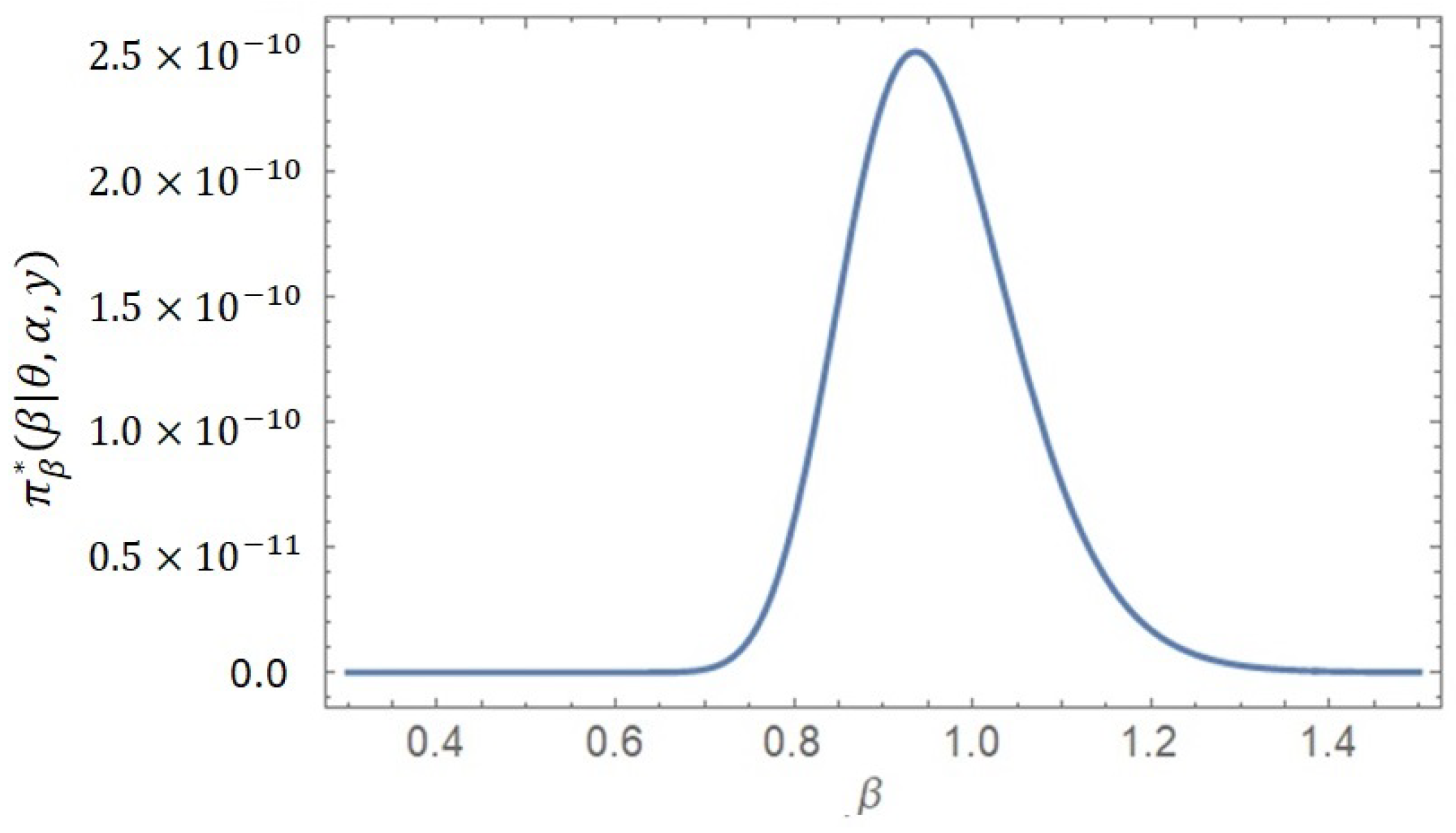
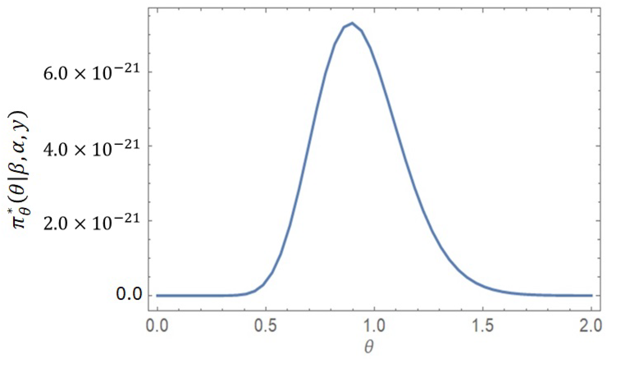
Figure 11, Figure 12 and Figure 13 show the conditional posteriors of $\theta ,\beta$, and $\alpha$.

The proposed PR accelerated life model is particularly suitable for accelerated life testing experiments conducted under step-stress acceleration with Type-I GHCS. Its performance is expected to be most effective when the underlying lifetime data exhibit characteristics consistent with the PR distribution and incomplete lifetime observations arise from censoring.

4.2. Simulation Analysis

A Monte Carlo simulation study was conducted to evaluate and compare the efficiency of the proposed Bayesian and MLE using the PR distribution. The parameter values used in the simulation studies are selected to ensure an optimal density-function shape. The censoring schemes considered in this simulation study were chosen to reflect practical accelerated life testing conditions and to evaluate the performance of the proposed estimation methods under different settings. The real values of the parameters were set to $(\theta ,\beta ,\alpha )=(0.8,0.6,2)$, and the significance level was established at $\nu =0.05$. Within the Type-I GHCS framework, the selection of $\theta$ and $\beta$ was informed by the analysis presented in Figure 1.

Two distinct sets of priors were considered parameters. The first set, Prior 1 (P1), represents an NIP scenario using diffuse gamma priors with hyperparameters of $a=b=c=d=0.0001$. The goal of these uninformative priors is to have as little impact as possible on the inference process so that the posterior distribution is dominated by the data’s likelihood. This approach is frequently utilized to ensure unbiased estimation in the absence of reliable prior information.

In the informative prior (IP) setting (P2), the hyperparameters were set to $a=b=c=1$ and $d=2$. These values were selected so that the corresponding prior means, i.e., $E\left(\theta \right)\cong a/b$ and $E\left(\beta \right)\cong c/d$, were consistent with the true parameter values used in the simulation study. This choice provides a moderately informative prior specification, allowing the Bayesian estimators to be evaluated under a realistic prior setting while maintaining a balance between prior information and the observed data. Estimator performance was assessed via 1000 Monte Carlo samples from the PR distribution (Algorithm 3). Average bias and MSE values are reported in

Table 5. Point estimation performance: average bias and MSE of $\theta$ at $(\theta ,\beta ,\alpha )=(0.8,0.6,2.0)$.

		MLE				Bayes (P1)				Bayes (P2)
($\mathit{n},\mathit{r},\mathit{k}$)	$\mathit{\tau },\mathit{T}$	Bias	MSE	AL	CP	Bias	MSE	AL	CP	Bias	MSE	AL	CP
(60, 40, 30)	0.8, 1.5	0.0052	0.0215	0.5102	0.965	0.0054	0.0272	0.4120	0.968	0.0034	0.0172	0.3907	0.970
	1, 1.5	0.0055	0.0218	0.5210	0.958	0.0055	0.0275	0.4018	0.954	0.0036	0.0118	0.3852	0.964
	0.8, 1.3	0.0061	0.0220	0.5429	0.960	0.0052	0.0277	0.4129	0.968	0.0033	0.0116	0.3990	0.966
	1, 1.3	0.0060	0.0219	0.5321	0.958	0.0053	0.0278	0.4003	0.972	0.0035	0.0115	0.3852	0.972
(80, 50, 40)	0.8, 1.5	0.0054	0.0218	0.5218	0.970	0.0056	0.0265	0.4354	0.925	0.0037	0.0156	0.4010	0.965
	1, 1.5	0.0057	0.0220	0.5234	0.968	0.0051	0.0217	0.4218	0.954	0.0038	0.0126	0.4009	0.972
	0.8, 1.3	0.0063	0.0224	0.5464	0.964	0.0054	0.0204	0.4429	0.948	0.0035	0.0127	0.3915	0.968
	1, 1.3	0.0061	0.0223	0.5247	0.972	0.0051	0.0221	0.4348	0.963	0.0037	0.0131	0.3992	0.974

, while

Table 6. Point estimation performance: average bias and MSE of $\beta$ at $(\theta ,\beta ,\alpha )=(0.8,0.6,2.0)$.

		MLE				Bayes (P1)				Bayes (P2)
($\mathit{n},\mathit{r},\mathit{k}$)	$\mathit{\tau },\mathit{T}$	Bias	MSE	AL	CP	Bias	MSE	AL	CP	Bias	MSE	AL	CP
(60, 40, 30)	0.8, 1.5	0.0051	0.0220	0.5012	0.946	0.0051	0.0221	0.4800	0.958	0.0036	0.0127	0.4012	0.974
	1, 1.5	0.0053	0.0222	0.5111	0.954	0.0052	0.0225	0.4580	0.950	0.0035	0.0110	0.3990	0.958
	0.8, 1.3	0.0056	0.0219	0.5301	0.968	0.0051	0.0220	0.4448	0.947	0.0034	0.0115	0.3915	0.964
	1, 1.3	0.0061	0.0223	0.5100	0.918	0.0052	0.0222	0.4548	0.952	0.0033	0.0120	0.3925	0.918
(80, 50, 40)	0.8, 1.5	0.0053	0.0210	0.5011	0.952	0.0056	0.0265	0.4354	0.925	0.0037	0.0156	0.4010	0.965
	1, 1.5	0.0056	0.0212	0.5060	0.948	0.0051	0.0217	0.4218	0.954	0.0038	0.0126	0.4009	0.972
	0.8, 1.3	0.0060	0.0218	0.5127	0.968	0.0054	0.0204	0.4429	0.948	0.0035	0.0127	0.3915	0.968
	1, 1.3	0.0057	0.0211	0.5170	0.964	0.0051	0.0221	0.4348	0.963	0.0037	0.0131	0.3992	0.974

provides the coverage probabilities (CPs) and average lengths (ALs) for the interval estimations.

Specifically, an accelerated Type-I GHCS sample was generated using $n=60$, $b_r=45$, $k=40$, and $\alpha$ = 2.0, assuming a stress-change point of 0.6.

Algorithm 3: MSE and CP Simulation Initialization

1. Initialization: Create a Type-I GHCS from the PR distribution and fix the parameters $(\tau ,n,r,k)$. 2. Point Estimation: Obtain the MLEs and BEs (employing the SE loss function) for the unknown parameters. 3. Interval Estimation: Establish the asymptotic, bootstrap, and Bayesian credible intervals. 4. Iteration: Perform N independent replications of the above steps to generate a distribution of estimates. 5. Aggregation: Calculate the average Bias, MSEs, and CPs for each run to assess the estimators. 6. Reporting: Tabulate the summarized simulation results as provided in Table 5, Table 6 and Table 7. Utilizing the failure data obtained from the Type-I GHCS, we computed point estimates through ML and Bayesian approaches. For the latter, a chain of 11,000 MCMC samples was generated, utilizing a 1000-sample burn-in period. Non-informative priors were selected to represent a state of prior ignorance regarding the parameters. Table 5 and Table 6 provide the consolidated results of these analyses, which were conducted using the Mathematica 12 software package. From the tables, we can conclude: A clear visualization (Forest Plot) comparing ML Confidence Intervals against Bayesian credible intervals (both IP and NIP). This confirms your observation that Bayesian intervals often provide more robust coverage. A dynamic batch-simulator that runs hundreds of iterations across different sample sizes to illustrate how MSE naturally trends downward as sample size and effective test time grow. Allows you to adjust hyperparameters to see how “IP Bayes” surpasses ML methods when prior knowledge is properly incorporated.

Table 7. Point estimation performance: average bias and MSE of $\alpha$ at $(\theta ,\beta ,\alpha )=(0.8,0.6,2.0)$.

		MLE				Bayes (P1)				Bayes (P2)
($\mathit{n},\mathit{r},\mathit{k}$)	$\mathit{\tau },\mathit{T}$	Bias	MSE	AL	CP	Bias	MSE	AL	CP	Bias	MSE	AL	CP
(60, 40, 30)	0.8, 1.5	0.1250	0.1520	1.2087	0.947	0.1186	0.1482	1.3201	0.952	0.1109	0.1219	1.1410	0.968
	1, 1.5	0.1154	0.1482	1.3289	0.954	0.1118	0.1441	1.3105	0.956	0.1001	0.1369	1.0163	0.970
	0.8, 1.3	0.1244	0.1520	1.2049	0.962	0.1215	0.1493	1.3018	0.954	0.1013	0.1334	1.1146	0.974
	1, 1.3	0.1186	0.1447	1.53258	0.954	0.1201	0.1486	1.4591	0.914	0.0998	0.1318	1.3569	0.968
(80, 50, 40)	0.8, 1.5	0.1310	0.1657	1.3180	0.954	0.1341	0.1667	1.4193	0.948	0.1218	0.1587	1.2185	0.962
	1, 1.5	0.1419	0.1663	1.3110	0.950	0.1385	0.1644	1.5019	0.928	0.1200	0.1499	1.0150	0.974
	0.8, 1.3	0.1318	0.1648	1.3480	0.918	0.1341	0.1632	1.4801	0.944	0.1218	0.1521	1.1020	0.970
	1, 1.3	0.1337	0.1654	1.4700	0.926	0.1319	0.1648	1.4218	0.938	0.1180	0.1541	1.1096	0.964

Table 7. Point estimation performance: average bias and MSE of $\alpha$ at $(\theta ,\beta ,\alpha )=(0.8,0.6,2.0)$.

		MLE				Bayes (P1)				Bayes (P2)
($\mathit{n},\mathit{r},\mathit{k}$)	$\mathit{\tau },\mathit{T}$	Bias	MSE	AL	CP	Bias	MSE	AL	CP	Bias	MSE	AL	CP
(60, 40, 30)	0.8, 1.5	0.1250	0.1520	1.2087	0.947	0.1186	0.1482	1.3201	0.952	0.1109	0.1219	1.1410	0.968
	1, 1.5	0.1154	0.1482	1.3289	0.954	0.1118	0.1441	1.3105	0.956	0.1001	0.1369	1.0163	0.970
	0.8, 1.3	0.1244	0.1520	1.2049	0.962	0.1215	0.1493	1.3018	0.954	0.1013	0.1334	1.1146	0.974
	1, 1.3	0.1186	0.1447	1.53258	0.954	0.1201	0.1486	1.4591	0.914	0.0998	0.1318	1.3569	0.968
(80, 50, 40)	0.8, 1.5	0.1310	0.1657	1.3180	0.954	0.1341	0.1667	1.4193	0.948	0.1218	0.1587	1.2185	0.962
	1, 1.5	0.1419	0.1663	1.3110	0.950	0.1385	0.1644	1.5019	0.928	0.1200	0.1499	1.0150	0.974
	0.8, 1.3	0.1318	0.1648	1.3480	0.918	0.1341	0.1632	1.4801	0.944	0.1218	0.1521	1.1020	0.970
	1, 1.3	0.1337	0.1654	1.4700	0.926	0.1319	0.1648	1.4218	0.938	0.1180	0.1541	1.1096	0.964

5. Concluding Remarks

Researchers may occasionally be unable to obtain comprehensive data on failure times over brief periods of time in reliability studies or life testing. Higher stress levels might be necessary to shorten these tests’ durations and lower their cost. As a result, we used an accelerated life testing model with partial step stress. Additionally, to limiting the number of units tested, a traditional Type-I GHCS was used to help save time and money. In the context of an accelerated Type-I GHCS method, we examined the PR distribution. We addressed the estimation problem assuming unit lifetimes follow a power Rayleigh distribution. Both maximum-likelihood and Bayesian methods were used to obtain point estimates for the model parameters. Interval estimates were computed using asymptotic MLE, two bootstrap methods, and credible intervals. The Bayesian estimates were developed using the MCMC algorithm. To demonstrate the proposed methods, two numerical examples were provided. The results obtained using different estimation techniques were analyzed and compared through a Monte Carlo simulation study.

Future research may extend this study in several significant directions. From a methodological perspective, the proposed framework could be generalized to address one-sample prediction problems and alternative estimation approaches such as E-Bayesian, modified moment, and least-squares methods. Further investigation is also needed to determine optimal stress-loading schemes for the PR distribution within the context of experimental design. Moreover, the applicability of the study may be enhanced by considering different censoring schemes, including Type-I, joint, and hybrid censoring, as well as by examining non-constant stress patterns such as cyclic and progressive loading.

References

1. Lone, S.A.; Panahi, H. Estimation procedures for partially accelerated life test model based on unified hybrid censored sample from the Gompertz distribution. Eksploat. I Niezawodn. Maint. Reliab. 2022, 24, 427–436. [Google Scholar] [CrossRef] [Scilit]
2. Lone, S.A.; Panahi, H.; Shah, I. Bayesian prediction interval for a constant-stress partially accelerated life test model under censored data. J. Taibah Univ. Sci. 2021, 15, 1178–1187. [Google Scholar] [CrossRef] [Scilit]
3. Degroot, M.H.; Goel, P.K. Bayesian and optimal design in partially accelerated life testing. Nav. Res. Logist. Q. 1979, 26, 223–235. [Google Scholar] [CrossRef] [Scilit]
4. Soliman, A.A.; Ahmed, E.A.; Abou-Elheggag, N.A.; Ahmed, S.M. Step-stress partially accelerated life tests model in estimation of inverse Weibull parameters under progressive Type-II censoring. Appl. Math. Inf. Sci. 2017, 5, 1369–1381. [Google Scholar] [CrossRef] [Scilit]
5. Fathi, A.; Farghal, A.W.A.; Soliman, A.A. Inference on Weibull inverted exponential distribution under progressive first-failure censoring with constant-stress partially accelerated life test. Stat. Pap. 2024, 65, 5021–5053. [Google Scholar] [CrossRef] [Scilit]
6. Ahmed, S.M. Constant-stress partially accelerated life testing for Weibull inverted exponential distribution with censored data. Iraqi J. Comput. Sci. Math. 2024, 5, 94–111. [Google Scholar] [CrossRef] [Scilit]
7. Ismail, G.M.; AAlqasem, O.A.; Alsolmi, M.M.; Alamoudi, L.M.; Habadi, M.I.; Ali Shiekh, R.H.; Rahman, M.M.; Ahmed, S.M. Statistical Inference for the Inverted Kumaraswamy Accelerated Model Under Type-I Generalized Hybrid Censoring with Applications. Symmetry 2026, 18, 446. [Google Scholar] [CrossRef] [Scilit]
8. Ismail, A.A. Reliability analysis under constant-stress partially accelerated life tests using hybrid censored data from Weibull distribution. Hacet. J. Math. Stat. 2016, 45, 181–193. [Google Scholar]
9. Hassan, A.S.; Assar, S.M.; Zaky, A.N. Constant-stress partially accelerated life tests for inverted Weibull distribution with multiple-censored data. Int. J. Adv. Stat. Probab. 2015, 1, 72–82. [Google Scholar] [CrossRef] [Scilit]
10. Kim, C.M.; Bai, D.S. Analysis of accelerated life test data under two failure modes. Int. J. Reliab. Qual. Saf. Eng. 2002, 9, 111–125. [Google Scholar] [CrossRef] [Scilit]
11. AL-Hussaini, E.K.; Abdel-Hamid, A.H. Accelerated life tests under finite mixture models. J. Stat. Comput. Simul. 2010, 76, 673–690. [Google Scholar] [CrossRef] [Scilit]
12. Wang, R.; Fei, H. Statistical inference of Weibull distribution for tampered failure rate model in progressive stress accelerated life testing. J. Syst. Sci. Complex. 2004, 17, 237–243. [Google Scholar]
13. Balakrishnan, N.; Aggarwala, R. Progressive Censoring: Theory, Methods and Applications; Birkhauser: Boston, MA, USA, 2000. [Google Scholar] [CrossRef] [Scilit]
14. Epstein, B. Truncated life test in exponential case. Ann. Math. Stat. 1954, 25, 555–564. [Google Scholar] [CrossRef] [Scilit]
15. Draper, N.; Guttman, I. Bayesian analysis of hybrid life tests with exponential failure times. Ann. Inst. Stat. Math. 1987, 39, 219–225. [Google Scholar] [CrossRef] [Scilit]
16. Gupta, R.D.; Kundu, D. Hybrid censoring schemes with exponential failure distribution. Commun. Stat. Theory Method 1998, 27, 3065–3083. [Google Scholar] [CrossRef] [Scilit]
17. Dube, B.; Pradhan, B.; Kundu, D. Parameter estimation of the hybrid censored log-normal distribution. J. Stat. Comput. Simul. 2010, 81, 275–287. [Google Scholar] [CrossRef] [Scilit]
18. Chandrasekar, B.; Childs, A.; Balakrishnan, N. Exact likelihood inference for the exponential distribution under generalized type-I and type-II hybrid censoring. Nav. Res. Logist. 2004, 51, 994–1004. [Google Scholar] [CrossRef] [Scilit]
19. Bhat, A.A.; Ahmad, S.P. A new generalization of Rayleigh distribution: Properties and applications. Pak. J. Stat. 2020, 36, 225–250. [Google Scholar]
20. Davison, A.C.; Hinkley, D.V. Bootstrap Methods and Their Application; Cambridge University Press: Cambridge, UK, 1997. [Google Scholar] [CrossRef] [Scilit]
21. Efron, B.; Tibshirani, R.J. An Introduction to the Bootstrap, 1st ed.; Chapman and Hall/CRC: New York, NY, USA, 1994. [Google Scholar] [CrossRef] [Scilit]
22. Robert, C.P.; Casella, G. Monte Carlo Statistical Methods, 2nd ed.; Springer: New York, NY, USA, 2004. [Google Scholar] [CrossRef] [Scilit]
23. Ahmed, S.M.; Ismail, G.M. Statistical Inference Based on Censored Data of Entropy for Lomax Distribution. Eur. J. Pure Appl. Math. 2025, 18, 5737. [Google Scholar] [CrossRef] [Scilit]
24. Nicholas, M.D.; Padgett, W.J. A bootstrap control for Weibull percentiles. Qual. Reliab. Eng. Int. 2006, 22, 141–151. [Google Scholar] [CrossRef] [Scilit]
25. Cordeiro, G.M.; Lemonte, A.J. The β-Birnbaum-Saunders distribution: An improved distribution for fatigue life modeling. Comput. Stat. Data Anal. 2011, 55, 1445–1461. [Google Scholar] [CrossRef] [Scilit]
26. Efron, B. Logistic regression, survival analysis, and the kaplan-meier curve. J. Am. Stat. Assoc. 1988, 83, 414–425. [Google Scholar] [CrossRef] [Scilit]
Figure 1. PDF of the PRD for different values of θ .
Mathematics 14 02447 g001
Figure 2. HRF of PRD for different values of θ .
Mathematics 14 02447 g002
Figure 3. The empirical and theoretical CDF of Application 1.
Mathematics 14 02447 g003
Figure 4. Histogram and trace of θ generated by MCMC for Application 1.
Mathematics 14 02447 g004
Figure 5. Histogram and trace of β generated by MCMC for Application 1.
Mathematics 14 02447 g005
Figure 6. Histogram and trace of α generated by MCMC for Application 1.
Mathematics 14 02447 g006
Figure 7. The empirical and theoretical CDF of Application 2.
Mathematics 14 02447 g007
Figure 8. Histogram and trace of θ generated by MCMC for Application 2.
Mathematics 14 02447 g008
Figure 9. Histogram and trace of β generated by MCMC for Application 2.
Mathematics 14 02447 g009
Figure 10. Histogram and trace of α generated by MCMC for Application 2.
Mathematics 14 02447 g010
Figure 11. The conditional posterior of θ (Application 2).
Mathematics 14 02447 g011
Figure 12. The conditional posterior of β (Application 2).
Mathematics 14 02447 g012
Figure 13. The conditional posterior of α (Application 2).
Mathematics 14 02447 g013