Article

IMU-Sequence-Based GNSS Short Outage Compensation and Hybrid Positioning Strategy

1
School of Automation, Wuhan University of Technology, Wuhan 430070, China
2
School of Mechanical Engineering, Hefei University of Technology, Hefei 230009, China
*
Author to whom correspondence should be addressed.
Mathematics 2026, 14(13), 2423; https://doi.org/10.3390/math14132423
Submission received: 16 May 2026 / Revised: 30 June 2026 / Accepted: 2 July 2026 / Published: 6 July 2026

Abstract

Pure inertial dead reckoning during short GNSS outages causes rapid drift on low-cost MEMS GNSS/IMU platforms. Most learning-based compensators upgrade a single predictor and rarely address late-outage drift or cross-domain bias mismatch. This paper proposes two enhancements over a Transformer baseline (TF-Base) plus a lightweight inference-time fusion strategy. MGTR (Motion-Guided Transformer with Tail-aware Readout) adds residual motion gating and a tail-aware readout for hard-segment and late-outage response. TAMS (Temporal Attention Multi-Scale) replaces global average pooling with learnable temporal attention and a short-window dual head. Delayed-Switch selects among TF-Base, MGTR, and TAMS without retraining backbones; its classifier needs a one-pass target-domain calibration, so it is not zero-shot. On real 5 Hz GNSS/IMU recordings under a three-tier protocol, where dead reckoning yields a 40.02 m mean RMSE on cross-domain segments, MGTR cuts the 90th-percentile 2D-RMSE by 20.3% over TF-Base, and Delayed-Switch reaches 30.32 m mean RMSE (24.2% below dead reckoning, 9.5% below TF-Base), within 0.51 m of the better-of-two upper bound. Against two recent baselines under the same protocol, only the AT-LSTM gain is significant after multiple-comparison correction; the margins over the strongest predictors are numerically favorable but not significant at this sample size, with gains concentrated on a few hard segments.

1. Introduction

Integration of the Global Navigation Satellite System (GNSS) with the Inertial Measurement Unit (IMU) underpins vehicle navigation and intelligent transportation applications. Vehicle trajectory data also supports scenario-based testing and safety assessment of intelligent vehicles [1]. In open environments, fusing GNSS measurements with IMU dead reckoning through a Kalman filter delivers continuous, stable position information [2,3,4]. Real urban traffic encounters short GNSS outages far more often than idealized testbeds suggest. Urban canyons, overpasses, tunnel entries, parking-structure pillars, and dense tree canopies cause complete signal loss or severe degradation for tens of seconds [2,5,6,7,8], and a typical commute encounters several such outages. Once GNSS measurements drop out, the system degrades to pure inertial dead reckoning, and the bias drift and random walk of low-cost MEMS accelerometers and gyroscopes accumulate tens of meters of two-dimensional positioning error within 10 to 30 s, threatening navigation continuity. Suppressing inertial drift during short GNSS outages while maintaining usable positioning accuracy thus remains an open engineering problem on low-cost vehicular platforms. The goal of this paper is to reduce the drift that pure inertial dead reckoning accumulates before the signal returns, using only the low-cost GNSS and IMU hardware already on board. Lane-level or safety-critical accuracy is not targeted, since a low-cost MEMS IMU cannot maintain it without satellite signals.
Research on suppressing positioning errors during GNSS outages follows two main lines. Traditional approaches restrict inertial dead reckoning errors through integrated filtering, kinematic constraints such as nonholonomic motion or zero velocity updates, or auxiliary sensors including odometers, LiDAR, and vision [6,8,9,10,11,12]; recent work also improves the integration itself, e.g., robust time synchronization for low-cost sensors [13] and 3-D grid-based pseudorange-error prediction in urban areas [14]. These methods perform well in structured scenarios but rely on extra hardware or strong platform priors, which limits direct application to vehicles equipped with only low-cost GNSS and IMU. Learning-based compensation has progressed rapidly in recent years. Early work combines deep learning with an improved EKF and uses multiple LSTM modules to predict position increments during outages [3]. Subsequent studies introduce CNN–LSTM compensators for ultra-low-cost IMUs [15], GRU+AKF hybrid algorithms [16], CNN-GRU+CKF in-vehicle implementations [17], and LSTM with factor graphs and cascade-LSTM methods aligned with realistic road conditions [18,19,20]. Newer methods such as AT-LSTM, CNN-GRU with IRAKF, and multidimensional hybrid position compensation further improve accuracy under real outage conditions [21,22,23]. More recent work explores semi-supervised Transformers, FECAM-iTransformer based on the iTransformer architecture [24], and dual-domain deep networks [25,26,27,28]. These models leverage self-attention and richer temporal representations to capture long-range dependencies and multivariate coupling; a recent review of neural networks for navigation summarizes the broader progress [5]. The literature collectively shows that learning-based compensation is gaining acceptance for GNSS outage scenarios. The pertinent question is no longer which sequence model to adopt but how to achieve further error reduction through more targeted algorithmic improvements once an effective predictor backbone is established.
Although learning-based methods reduce positioning errors during outages, several weaknesses persist when the physical characteristics of inertial drift are examined closely. Pure dead reckoning error accumulates with outage duration, so late-stage drift is harder to suppress than the early stage. Existing temporal models, including the global average pooling readout in Transformers, weight all time steps equally. High-curvature maneuvers amplify gyroscope bias yet most current methods lack explicit motion-aware mechanisms. Different scenarios—straight versus turning, short versus long—place differing demands on the compensator, and a single model rarely dominates every condition; complementarity among improvement strategies is seldom studied. To address these issues, we adopt a Transformer encoder TF-Base (compared with an LSTM baseline) and propose two targeted enhancements, MGTR and TAMS, together with an inference-time strategy, Delayed-Switch, that selects between them per segment without retraining backbones. Compared with recent single-predictor compensators such as CNN-GRU, AT-LSTM, and iTransformer-based hybrids [17,21,26], this paper differs in two ways: MGTR and TAMS add mechanisms that explicitly target late-outage drift and hard segments (motion gating, tail-aware and attention readouts), and Delayed-Switch adds an inference-time per-segment selection layer that needs no backbone retraining, a direction that has received little attention in the single-predictor literature. The full pipeline is validated on two datasets collected on different days with a low-cost MEMS GNSS/IMU module, covering straight and turning segments at varying speeds on urban roads. The main contributions of this work are summarized as follows.
  • Two targeted improvements for late-outage drift and hard-segment compensation: Recent compensators keep a generic equal-weight readout and no motion prior; MGTR adds a gyroscope-gated residual branch and a tail-aware readout, and TAMS replaces uniform pooling with learned temporal attention and a short-window mean. MGTR cuts the cross-domain P90 by 20.3% (65.41 m to 52.12 m), with the gain concentrated on hard segments (mean RMSE 16.6 % on the upper P75 quartile); TAMS improves the cross-domain mean RMSE by 5.3%. MGTR is stronger on mean RMSE and P90, whereas TAMS leads on T abs @ 5  m (6.3 s vs. 5.6 s) and median RMSE, so the two methods provide differentiated branches for the strategy layer.
  • Delayed-Switch as a lightweight inference-time hybrid strategy: Rather than deploying one predictor across all scenarios, Delayed-Switch selects among frozen backbones per segment: the first T 0 = 6  s of an outage uses TF-Base, then a classifier (calibrated once on a disjoint development split of the target domain, i.e., not zero-shot) selects between MGTR and TAMS for the rest; the cross-domain mean RMSE on the 24 held-out segments reaches 30.32 m, a 24.2% reduction from pure inertial dead reckoning (40.02 m) and a 9.5% reduction from TF-Base (33.52 m).
  • Real-vehicle empirical study on low-cost MEMS IMUs with a three-tier evaluation protocol: Two datasets collected on different days with a low-cost MEMS GNSS/IMU module covering urban roads support a three-tier evaluation: same-domain validation on three fixed segments → Monte Carlo stress test on 24 randomly sampled segments → cross-domain held-out evaluation on 24 segments.
The remainder of the paper is organized as follows. Section 2 reviews related work. Section 3 details the system structure and theoretical formulation of the proposed algorithms. Section 4 presents the experimental configuration, datasets and results for each contribution. Section 5 concludes the paper and outlines future work.

2. Related Work

GNSS/IMU integrated positioning has long relied on filtering and multi-source fusion to suppress inertial drift. Groves et al. [9] summarize the integration challenges of advanced multi-sensor navigation systems and argue that future systems must pursue accuracy, robustness, and modular extensibility under demanding environments; GNSS modeling for urban environments and low-cost multi-sensor augmentation studies further reflect the same direction [4,7]. Traditional approaches typically introduce stronger prior constraints or auxiliary sensors to improve integrated positioning. Gao et al. [10] use dual odometers to refine SINS/OD integration on ground vehicles, while Wang et al. [11] apply 3D LiDAR for GNSS/INS fault detection and adaptive filtering in urban canyons. Gu et al. [6], Sun et al. [8], and Niu et al. [12] demonstrate that tightly coupled visual–inertial–GNSS systems remain effective in degraded urban GNSS environments. These approaches perform well in structured scenarios, yet their dependence on platform-specific assumptions, extra hardware, or complex system configurations limits applicability to short-outage compensation that relies solely on low-cost GNSS and IMU.
To reduce dependence on extra hardware and strong model priors, research shifts toward learning-based compensation. Early work directly learns the mapping between INS measurements and GNSS position increments through neural networks or support vector regression. For instance, Sharaf et al. [29] use an RBF network for online INS/GPS aiding, Tan et al. [30] apply GA-SVR to predict pseudo-positions during outages, and Yao et al. [31] combine pseudo-measurement prediction with filtering for outage compensation. Hybrid methods such as CKF-MLP and RBF-CKF also compensate position and velocity errors during outages [32]. In the deep learning era, LSTM [33] and GRU became mainstream sequence modeling tools. Fang et al. [34] predict pseudo-GNSS position increments with an LSTM to aid the INS, Liu et al. [18] integrate an LSTM with a factor-graph back end [35] for natural GNSS outages on real roads, and Zhao et al. [19] adopt a CNN-GRU and factor-graph hybrid to improve robustness under frequent and persistent outages. Chen et al. [21], Meng et al. [22], and Zhang et al. [23] further advance this line through attention modeling, robust adaptive filter coupling, and multidimensional position compensation. More recent studies continue this single-predictor line but under settings different from ours: an LSTM with a feature-pyramid network for bridging long 30–180 s outages [36], a robustness study of LSTM and gradient-boosting positioning under noisy and biased inputs [37], a PSO-optimized LSTM with a fading adaptive filter for extended outages [38], and a cascaded LSTM with variational Bayesian filtering for minute-scale GNSS-denied navigation [39]. Because these differ from our short single-outage, online setting in outage length or filter back end, our experimental comparison instead focuses on the protocol-compatible recent baselines reproduced in Section 4.5. These works show that learning-based pseudo-measurement generation on a single predictor is an effective route, while their core improvement still revolves around replacing that predictor with a stronger one.
Recent work has shifted toward the Transformer [40] and stronger sequence modeling architectures. Wang et al. [25] propose an online semi-supervised Transformer that improves GNSS/INS navigation resilience under bounded computational budgets. Guyard et al. [27] reconstruct trajectories after GNSS outages by modeling velocity with a Transformer encoder followed by bidirectional integration, illustrating the potential of Transformers. Kuang and Yan [26] combine the iTransformer [24] with FECAM and generate pseudo-GNSS increments through channel-correlation modeling and frequency-domain enhancement. The DDMNet framework extends to a unified system design jointly addressing dual-domain feature modeling, adaptive filtering, and validation under real outages [28]. A CNN–Transformer hybrid has likewise been applied to GNSS/RISS integration during outages [41], on a reduced inertial sensor suite different from our low-cost MEMS setting. The current question is no longer whether to introduce a Transformer but how targeted improvements can address concrete weaknesses such as accelerated late-outage drift and weak response to highly dynamic scenarios, thereby improving error suppression, hard-segment response, and substitution time.
In summary, prior work evolves from conventional filtering and constraint-based approaches to RNN, GRU, and Transformer predictors (Table 1). Compared with the dominant route of replacing or strengthening a single predictor, dedicated solutions remain rare that address late-outage drift and limited scenario adaptability through motion-aware and temporal-adaptive modeling while systematically analyzing their complementarity. Building on TF-Base, this paper proposes MGTR, which fuses motion-guided gating with tail-aware readout to suppress hard-segment errors, and TAMS, which improves sequence modeling through temporal attention pooling and dual-head residual prediction. The focus lies in designing tailored improvements for concrete weaknesses in outage compensation and validating their practical benefit on real low-cost vehicular data. The subsequent sections build on these results to introduce an inference-time strategy layer for further refinement. The differences from the three categories above can be stated directly. The Transformer line strengthens the sequence model itself, through semi-supervised updating, frequency-domain channel modeling, or bidirectional reconstruction, but keeps a generic readout that weights all time steps equally and uses no motion prior; MGTR and TAMS keep the encoder unchanged and modify exactly these two parts, with a gyroscope-gated residual branch and tail-aware or attention readouts aimed at late-outage drift and turning segments. The LSTM/GRU line and its filter hybrids upgrade the predictor or couple it with an adaptive filter, and the attention they add, as in AT-LSTM, is learned from hidden states alone; the gating used here is driven instead by physical motion channels (angular rate, cumulative heading change, speed). Finally, all of these methods deploy one predictor for every scenario, whereas Delayed-Switch selects among three frozen predictors per segment at inference-time, calibrated once on a development split and with no backbone retraining. Section 4.5 reproduces AT-LSTM and CNN-GRU under the same protocol to quantify these differences.

3. Materials and Methods

3.1. System Overview

The proposed framework targets short GNSS outages on low-cost MEMS GNSS/IMU platforms by feeding a sliding window of IMU dead reckoning features into a sequence model that outputs an online drift correction. Its inputs, processing components, and outputs are summarized as follows. The overall pipeline is illustrated in Figure 1.
Inputs. A 50 × 12 window sampled at 5 Hz: ENU dead reckoning position (3 dim.), raw accelerometer (3 dim.), raw gyroscope (3 dim.), cumulative heading change, dead reckoning speed, and elapsed time since outage start (1 dim. each). Transformer variants prepend 8 sinusoidal positional encoding dimensions, giving a 20 dim. augmented input. Windows shorter than 50 steps at outage onset are left-padded with zeros, identically in training and inference (Section 3.2).
Components. (i) An ESKF baseline that fuses GNSS and IMU during availability and reverts to heading-constrained dead reckoning at outage; (ii) two single-architecture baselines, an LSTM and a Transformer encoder TF-Base (Section 3.2); (iii) two TF-Base-based enhancements, MGTR with residual motion gating and tail-aware readout (Section 3.3) and TAMS with temporal attention pooling and dual-head residual prediction (Section 3.4); (iv) the Delayed-Switch inference-time strategy layer (Section 3.5) that conditionally selects MGTR or TAMS after a 6 s warm-up.
Outputs. A 5 dim. label [ ψ , v , z , e 10 , n 10 ] whose first three dimensions correct the dead reckoning trajectory online; the unified label, z-score normalization, and MSE loss are defined in Section 3.2.
The end-to-end data flow is summarized in Figure 1.

3.2. Backbones and Training Setup

ESKF and IMU dead reckoning. The positioning baseline follows a standard error state Kalman filter that loosely couples GNSS and IMU during availability [42]. The error state covers position, velocity, attitude, and the accelerometer and gyroscope biases; the process-noise covariance is built from accelerometer and gyroscope noise parameters of 1 ( m / s 2 ) 2 and 0.01 ( rad / s ) 2 and bias random walk parameters of 10 2 and 10 3 , and the GNSS measurement noise is 2.0 m 2 horizontally and 10.0 m 2 vertically; these values were tuned once on Dataset 1 and reused unchanged on Dataset 2. The filter initializes at the first GNSS fix with zero velocity, and all positions are expressed in a local ENU frame anchored at the Dataset 1 origin. On Dataset 1, the filter reduces the 2D positioning RMSE from 3.57  m of raw GNSS to 3.30  m (a 7.8 % improvement), and the fused trajectory replaces raw GNSS as the positioning baseline for outage experiments. During an outage, the GNSS measurement is disconnected and the system reverts to a 2D heading-speed dead reckoning model: the initial heading ψ 0 uses the GNSS displacement difference heading at outage start (with GNSS yaw and IMU AngleZ as fallbacks), subsequent updates apply ψ k = ψ 0 + ψ AngleZ , k , and forward acceleration integrates to a non-negative scalar speed v k = max ( v k 1 + a forward , k t , 0 ) . The horizontal position propagates by
e k = e k 1 + v k sin ψ k t , n k = n k 1 + v k cos ψ k t ,
with t = 1 / f s = 0.2  s and f s = 5  Hz; the vertical channel reads the barometer, calibrated to the GNSS altitude at outage start. This trajectory and its raw IMU statistics form the input feature window of the neural drift correction.
LSTM baseline. The classical LSTM [33] serves as the first temporal baseline; the standard gated cell is widely adopted for GNSS/INS outage compensation [18,21,34] and is not detailed here. Online inference during an outage cannot access future data, so the model uses a 50-step input window (10 s at 5 Hz) with a lightweight configuration: a single-layer unidirectional LSTM of hidden size 64 followed by an MLP regression head ( 64 32 5 , ReLU and Dropout 0.2 between layers); the MLP avoids the representation bottleneck of regressing directly from h T . Only the first three outputs are used at inference, with the 5 dim. label following Section 3.1.
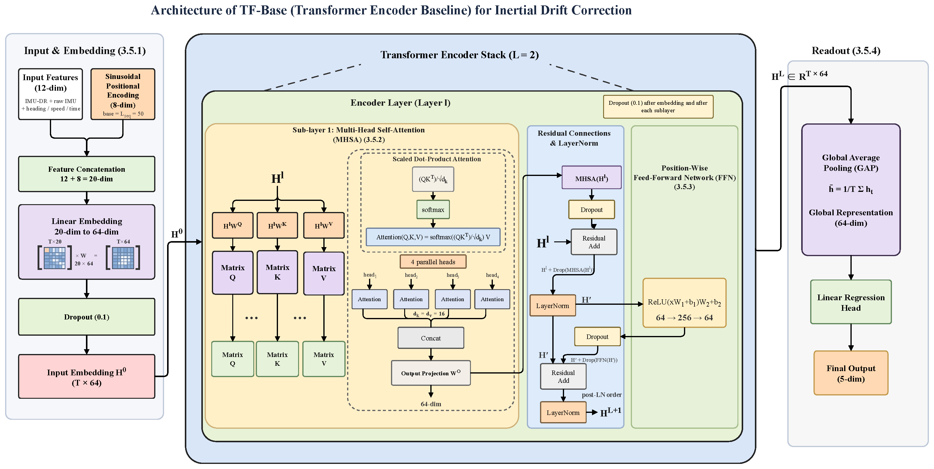
TF-Base. Each LSTM step depends on the previous hidden state, which limits long-range temporal modeling. The Transformer [40] uses self-attention to globally associate any two time steps in a single pass; in inertial drift correction, the current drift depends on both recent motion (e.g., turns in the last few steps) and earlier history (e.g., the heading bias at outage start), so non-local modeling fits the task. The Transformer encoder therefore serves as the second baseline TF-Base and as the backbone for the subsequent improvements. Since the encoder follows the standard Transformer design, its layer-level diagram is provided in Appendix D (Figure A3).
TF-Base inherits the standard three-stage encoder structure (input embedding, encoder stack, GAP readout with regression head) [40]. Three task-specific configurations adapt to the short window L seq = 50 steps (10 s at 5 Hz): the positional encoding uses 8 sinusoidal dimensions concatenated with the 12 dim. IMU features (20 dim. input), with the frequency base changed from 10,000 to L seq so most components retain non-trivial periodicity within the window; the encoder has L = 2 Post-LN layers, h = 4 MHSA heads ( d k = d v = 16 ), d model = 64 , and FFN d ff = 4 d model = 256 ; and dropout 0.1 is applied after the embedding and each sublayer.
The GAP readout averages the encoder output H L R T × d model uniformly along the time axis, h ¯ = T 1 t = 1 T h t , before a linear head produces the 5 dim. output. LSTM and TF-Base have about 22K and 102K parameters respectively, both within O ( 10 5 ) ; the modular encoder structure also eases the injection of motion gating and temporal attention in the next two sections.
All learning models share the same training data, label, normalization, and loss for fair comparison. The 3 dim. current-step drift correction [ ψ , v , z ] and the 2 dim. east/north endpoint residual [ e 10 , n 10 ] at 10 s ahead form a unified 5 dim. label
y = [ ψ , v , z , e 10 , n 10 ] R 5 ,
whose first three dimensions correct the dead reckoning trajectory at inference and whose last two only supervise medium-to-long-term error trends offline. Because the dimensions have heterogeneous physical units (degrees, m/s, m), labels and inputs are z-score-normalized using the training set mean μ d and standard deviation σ d , y ˜ d = ( y d μ d ) / σ d . All models then minimize the unified MSE loss in the normalized space
L = 1 2 N i = 1 N y ˜ ^ i y ˜ i 2 = 1 2 N i = 1 N d = 1 5 y ^ i , d y i , d 2 σ d 2 ,
which is equivalent to an inverse-variance weighted MSE on the original labels and removes manual per-dimension weighting. To check whether the two auxiliary dimensions help, TF-Base was retrained with only the 3 dim. online label under the identical protocol (three runs, representative selected by validation RMSE). The result is a cross-domain mean RMSE of 33.15 m for the 3 dim. label versus 33.52 m for the 5 dim. label, comparable on this metric (signed-rank p = 0.44 , 95% bootstrap CI [ 4.22 , 2.41 ]  m), while the 5 dim. variant keeps a slightly longer substitution time (6.1 versus 5.5 s); neither difference is significant. The auxiliary supervision is therefore not critical to the online 2D metrics; its effect is within the seed-level variability reported in Appendix B. The 5 dim. label is kept so that all compared models share the same label interface and for offline trend analysis.
Online inference protocol. During an outage, every compensator runs once per t = 0.2  s step from the outage onset. At step t i , the input window covers the min ( t i , 50 ) most recent intra-outage steps; before the 50-step (10 s) window fills, the window is left-padded with zeros so that the real steps stay right-aligned. The identical padding is applied when generating training windows, so the training and inference input distributions match. No pre-outage buffer, warm start, or future information is used, and each step requires a single forward pass with negligible latency relative to the 0.2 s sampling interval. Consequently, the Delayed-Switch decision at T 0 = 6  s (Section 3.5) operates on a window of 30 real steps plus 20 zero-padded steps, using online signals only.

3.3. MGTR: Motion-Guided Improvement for Late-Outage Drift and Hard Segments

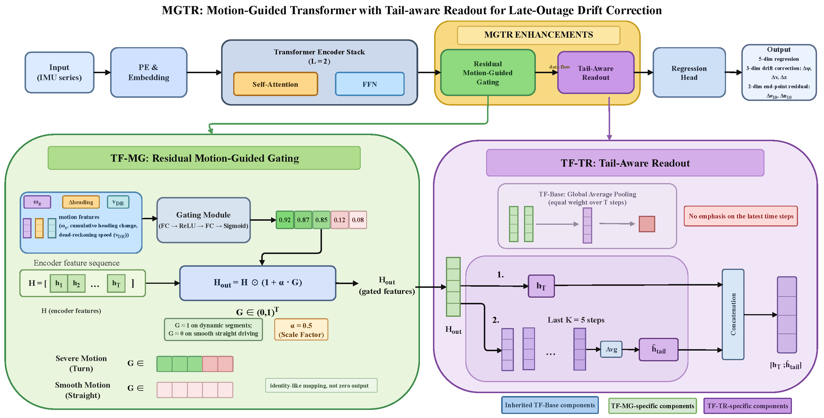
The baseline comparison in Section 4.2 shows that LSTM and TF-Base have similar overall capability, yet either single baseline falls short on hard segments and during the late half of an outage. Cross-domain T abs @ 5  m drops sharply from 21.8 s in the same domain to 6.1 s, indicating that the uniform-weight GAP readout poorly suppresses late-outage drift under cross-domain hard conditions. Pure inertial error accumulates with outage duration so late drift is harder to suppress, and high-curvature maneuvers amplify gyroscope bias. To address both, MGTR injects a tail-aware readout and a motion-guided gating mechanism into the TF-Base encoder (Figure 2).
The input embedding (12 dim. IMU features plus 8 dim. sinusoidal positional encoding) and the L = 2 Post-LN encoder stack ( h = 4 heads, d model = 64 , d ff = 256 ) are reused unchanged from Section 3.2; the two improvements below are inserted between the encoder and the regression head and replace the GAP readout.
Improvement 1: TF-MG (motion-guided gating). TF-MG selects three motion-relevant channels—the gyroscope z-axis angular rate ω z , the cumulative heading change, and the dead reckoning speed v DR —and a two-layer MLP (FC, ReLU, FC, sigmoid) produces a per-step gating signal G ( 0 , 1 ) T that modulates the encoder output through
H out = H ( 1 + α · G ) ,
with α = 0.5 and ⊙ element-wise. The residual form 1 + α G keeps smooth steps near identity ( H out H ) and emphasizes dynamic steps where gyroscope bias dominates.
Improvement 2: TF-TR (tail-aware readout). TF-TR (Last+TailMean) replaces the GAP readout: h T and the mean of the last K = 5 steps h ¯ tail are concatenated along the feature dimension, h readout R 2 d model , and fed to the regression head. Unlike GAP, which weighs all time steps equally, this readout keeps the focus on the terminal hidden states, which carry the drift information that matters most late in an outage. K = 5 (the last 1 s at 5 Hz) trades smoothing the instantaneous noise of h T against keeping the tail focus; the larger K = 10 in TAMS (Section 3.4) serves a different recent-scale purpose.
MGTR adds TF-MG and TF-TR to TF-Base, contributing ∼13K parameters at O ( T d model ) extra cost (∼4K from the TF-MG MLP gate, ∼9K from the 128 64  TF-TR head).

3.4. TAMS: Temporal Attention Improvement for Adaptive Sequence Modeling

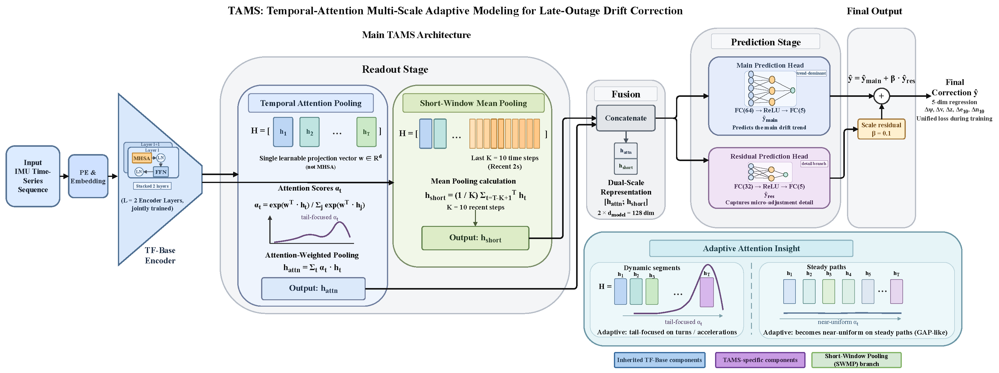
TAMS (Temporal Attention Multi-Scale) shares the TF-Base encoder backbone with MGTR but takes a complementary approach: instead of explicit motion priors, it lets learnable parameters decide which time steps and which scale matter most. Three mechanisms compose the algorithm—temporal attention pooling, short-window mean pooling, and dual-head residual prediction—concentrated on the readout and prediction stages while the encoder remains unchanged (Figure 3).
The input embedding and the L = 2 Post-LN encoder stack are reused unchanged from Section 3.2; the three improvements below redesign only the readout and prediction stages, and unlike MGTR, no motion-gating module is inserted into the encoder.
Improvement 1: temporal attention pooling. TAMS introduces a learnable projection vector w R d model that, via softmax over the encoder output H = [ h 1 , , h T ] , weighs time steps to form a global representation h attn :
α t = exp ( w h t ) j = 1 T exp ( w h j ) , h attn = t = 1 T α t h t , h short = 1 K t = T K + 1 T h t .
A single learnable vector (rather than full MHSA) keeps readout parameters small while still letting the model decide which steps matter. The vector w is trained end-to-end with the same regression loss as the rest of the network; no separate training stage or auxiliary objective is involved.
Improvement 2: short-window mean pooling. In parallel, h short uniformly averages the last K = 10 steps (2 s at 5 Hz), and the two are concatenated as [ h attn ; h short ] R 2 d model to fuse global and recent dynamics. The larger K = 10 versus K = 5 in TF-TR (Section 3.3) reflects this branch’s recent-scale aggregation purpose rather than terminal-state approximation.
Improvement 3: dual-head residual prediction. The 128 dim. representation feeds two FC heads in parallel: the main head FC ( d model ) ReLU → FC ( 5 ) (hidden width 64) produces y ^ main for the dominant drift trend; the residual head FC ( d model / 2 ) ReLU → FC ( 5 ) (hidden width 32) produces y ^ res for fine-grained residuals. The final prediction is
y ^ = y ^ main + β y ^ res , β = 0.1 .
The residual scale β = 0.1 is distinct from the encoder gating coefficient α = 0.5 in TF-MG (Section 3.3); the temporal attention weights α t defined above carry a time index and denote per-step pooling weights, not this scalar gating coefficient.
MGTR and TAMS are not interchangeable refinements of the same idea; they target different sources of inertial error. MGTR’s residual motion gating uses the gyroscope z-axis as a fixed motion prior, so the gain G approaches one on segments with high angular activity and degenerates to identity on quasi-straight segments. It therefore amplifies the encoder response to the gyroscope bias accumulation induced by turning. TAMS instead lets the softmax temporal attention learn from data which time steps carry the strongest signal, so it adapts to the non-stationary build-up of inertial drift without committing to a specific motion channel. The two mechanisms address complementary physical regimes.

3.5. Delayed-Switch Inference-Time Strategy

MGTR uses fixed motion priors (gyroscope channel, terminal window K = 5 ), whereas TAMS leaves time step weighting and scale fusion to learnable parameters; this complementarity (Section 4.3) motivates an inference-time fusion strategy. All three backbones are trained once on Dataset 1 and remain frozen throughout; the strategy layer selects among their outputs and never updates their weights.
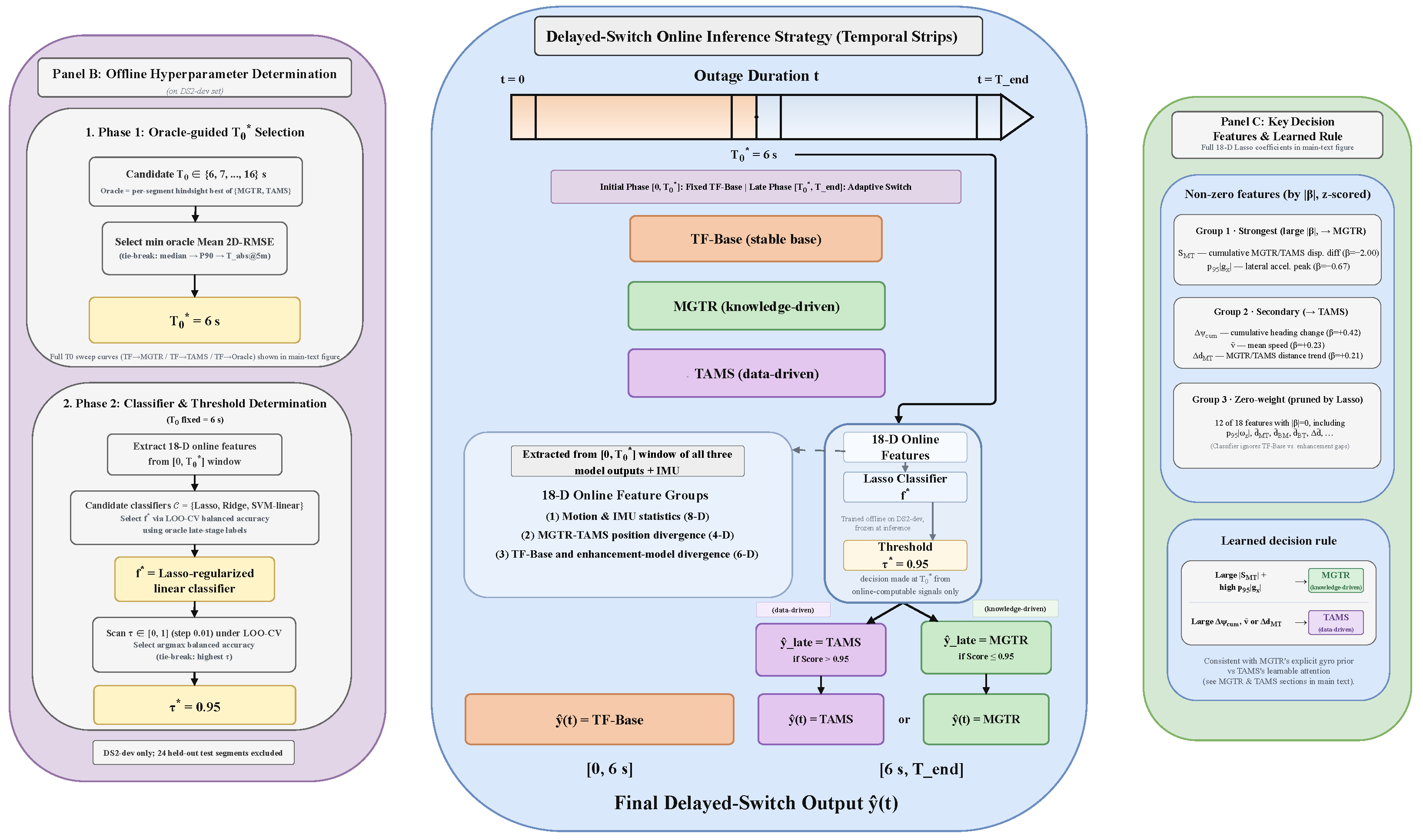
Delayed-Switch introduces no new neural network. At inference, a lightweight strategy layer conditionally switches between TF-Base, MGTR, and TAMS in three steps (Figure 4): (i) the first T 0 seconds use TF-Base for early-stage stability; (ii) at T 0 , an 18 dim. online feature vector (Table 2 and Table 3) feeds an 1 -regularized logistic regression classifier [43], referred to as the lasso classifier below; (iii) the chosen MGTR or TAMS prediction drives the remaining outage. All decisions use online signals only.
The 18 online features at switching time T 0 form three groups: motion and IMU statistics (8 dim., Table 2) describing first-stage vehicle dynamics; MGTR/TAMS positional disagreement (4 dim.) reflecting whether the two enhancements judge the scenario differently; and TF-Base/enhanced-model disagreement (6 dim.) capturing correction direction and amplitude relative to the baseline (the latter two groups in Table 3). All features depend only on the first T 0 seconds and introduce no backward delay.
These 8 features, together with the 10 inter-model disagreement features defined in Table 3, form an 18 dim. online feature vector x R 18 that feeds a logistic regression classifier trained with the lasso ( 1 ) penalty
min β 0 , β R 18 1 N i = 1 N log 1 + e y ˜ i ( β 0 + x i β ) + λ β 1 ,
where y ˜ i { 1 , + 1 } encodes the oracle label of development segment i ( + 1 = TAMS, 1 = MGTR, the branch with the smaller hindsight segment RMSE). This is a convex program. At the optimum, | j L log ( β ) | λ holds for every zero coordinate β j = 0 , and j L log ( β ) = λ sign ( β j ) otherwise, where L log is the average logistic loss. The 1 penalty induces structural sparsity: features weakly correlated with the second-stage label are driven to zero rather than retained with small weights, which yields a sparse classifier interpretable through its few non-zero coordinates and preserves the convexity of the underlying optimization problem. At inference the classifier outputs the posterior p TAMS ( x ) = σ ( β 0 + x β ) , with σ ( · ) the logistic function, and the decision rule defaults to TAMS: MGTR is selected only when p MGTR = 1 p TAMS τ .
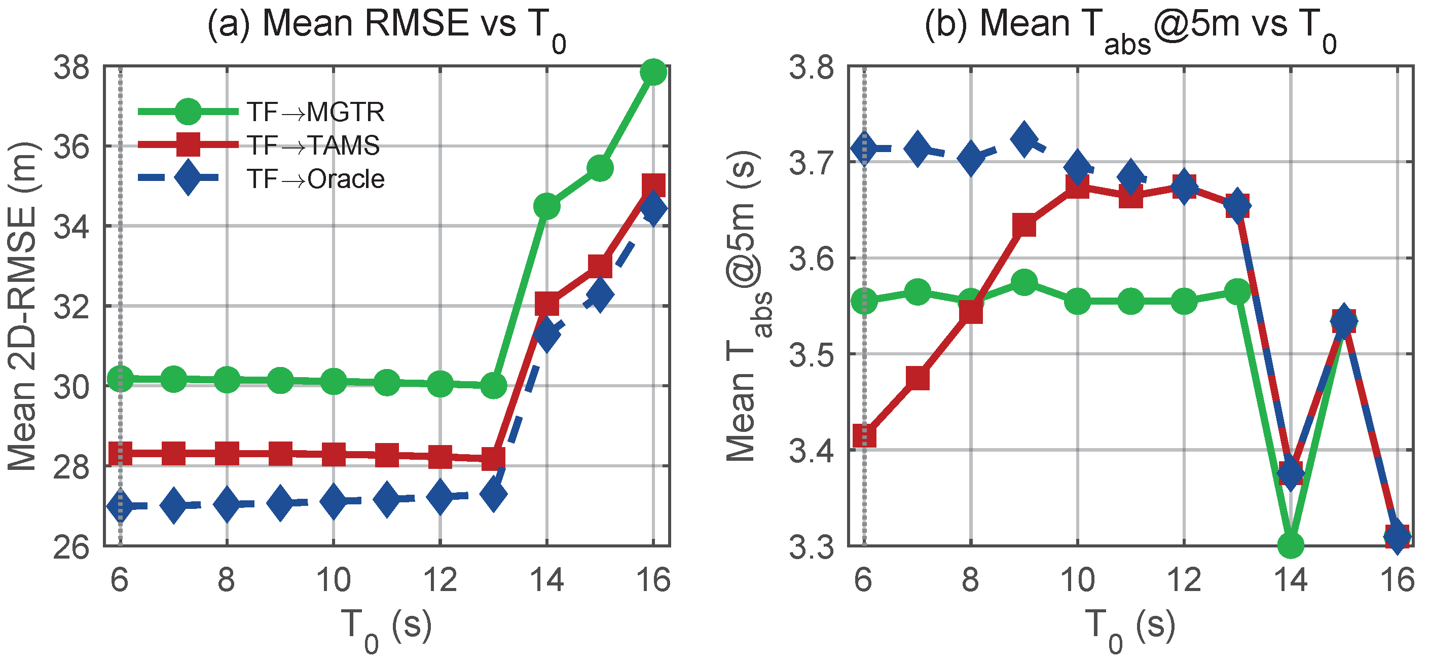
The strategy hyperparameters { T 0 , f , τ } are determined offline on DS2-dev (the 20 development segments of Dataset 2 after excluding the 24 held-out test segments). Stage one sweeps T 0 { 6 , 7 , , 16 }  s with oracle-guided per-segment selection from {MGTR, TAMS}, ties broken by median, P90, then T abs @ 5  m, yielding T 0 = 6  s (Figure 5). Stage two fixes T 0 = T 0 and extracts the 18 dim. features with oracle second-stage labels. It then selects the classifier f by LOO-CV balanced accuracy from a candidate set spanning regularized logistic regression ( 1 /lasso and 2 /ridge), discriminant analysis, decision trees, and bagged-tree ensembles; the 1 -logistic (lasso) model is selected. A step-0.05 scan over τ { 0.50 , 0.55 , , 0.95 } on the LOO-CV scores then yields τ = 0.95 , the largest member of the optimal set (ties resolved toward the most conservative value). The strategy is insensitive to this choice: the classifier scores on the held-out segments saturate near { 0 , 1 } , so every τ in the swept range gives the same test decisions (8 MGTR/16 TAMS) and the same mean RMSE of 30.32 m, identical to the maximum a posteriori rule. With { f , τ } frozen and the three backbones unchanged, final performance on the 24 cross-domain held-out segments is reported in Section 4.4. Delayed-Switch therefore relies on this one-pass target-domain calibration and is not a zero-shot method.
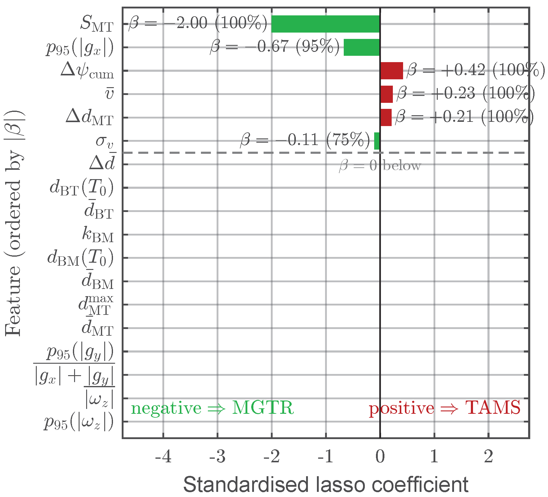
The lasso coefficients of the trained classifier (denoted β here, distinct from the residual scaling β = 0.1 in TAMS) are shown in Figure 6. After z-score normalization, lasso sparsification leaves six non-zero coefficients out of 18: S MT ( β = 2.00 ) and p 95 ( | g x | ) ( 0.67 ) favor MGTR; ψ cum ( + 0.42 ), v ¯ ( + 0.23 ), and d MT ( + 0.21 ) favor TAMS; σ v ( 0.11 ) favors MGTR. The TF-Base disagreement terms d ¯ BM and d ¯ BT are zero-weighted. Sign stability across DS2-dev 20-fold LOO retraining: the top-2 coefficients keep their sign in 100% and 95% of folds, and all top-5 in at least 75%.
During the first ∼10 s of an outage, the dead reckoning error is dominated by initial-condition uncertainty (heading at outage start, initial speed estimate) and the IMU bias has not yet accumulated significantly; all four neural compensators produce similar predictions because their outputs are largely set by the input window itself. After ∼10 s the integration of accelerometer and gyroscope biases becomes the dominant error source, and the architectural differences—motion gating in MGTR, temporal attention in TAMS—start to differentiate model outputs (Appendix C). This physical separation between an initial input-bound phase and a later drift-bound phase justifies a fixed initial phase rather than an immediate per-segment switch.

4. Results and Discussion

4.1. Experimental Setup

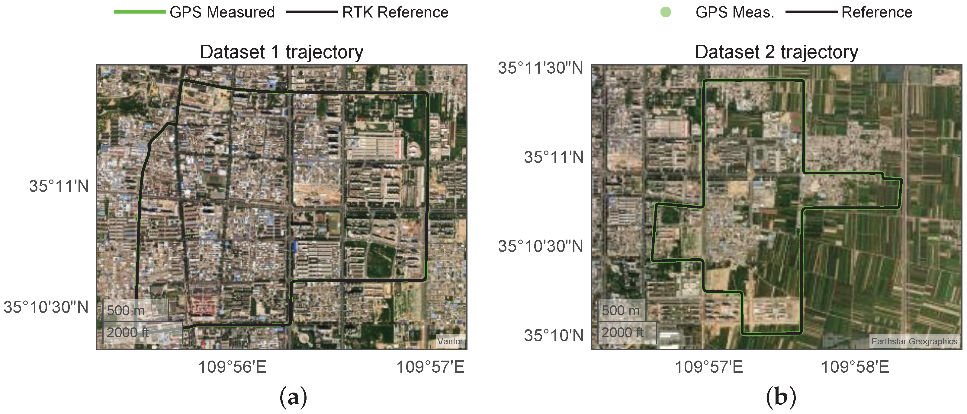
The experimental platform is Windows with MATLAB R2024b (Deep Learning Toolbox; The MathWorks, Inc., Natick, MA, USA). The acquisition platform consists of two independent GNSS receivers and a low-cost MEMS 10-axis IMU. The ESKF observation comes from the multi-constellation NMEA module of the HuanEr Technology IMU kit (HuanEr Technology Co., Ltd., Shenzhen, China), which uses GPS, BDS, and GLONASS and reaches meter-level single-point positioning. The ground truth is recorded through an independent serial interface from a Quectel LC29H dual-frequency GNSS/RTK module (Yunlu Information Technology Co., Ltd., Hefei, China) that provides centimeter-level fixed solutions of about 2.5 cm. The IMU has accelerometer range ±16 g, gyroscope range ±2000°/s, and a barometer with 0.5 Pa RMS. All three streams are time-synchronized and resampled to a unified 5 Hz; the residual synchronization error is bounded by the 0.2 s resampling grid, and dedicated synchronization methods for low-cost sensors are discussed in [13]. Throughout the paper, GNSS denotes the multi-constellation satellite service; the label “GPS” is retained in figure legends (following the receiver’s NMEA naming) and in established method or system names.
The unified training protocol applies to all neural networks: Adam ( β 1 = 0.9 , β 2 = 0.999 , ϵ = 10 8 ), initial learning rate 3 × 10 3 with 0.5 decay every 20 epochs, batch size 256, 50 epochs maximum. Inputs and outputs are z-score-normalized using training set statistics, applied identically at test time including the cross-domain test on Dataset 2. The loss is the unified 5 dim. MSE regression loss in z-score space defined in Section 3.2. TAMS is sensitive to random initialization through its attention pooling layer; five independent runs are performed and the representative model is selected by mean RMSE on the three fixed validation segments of Dataset 1. Appendix B additionally reports three independent training runs each for TF-Base and MGTR under the same protocol. The Delayed-Switch lasso classifier is trained offline with LOO-CV on DS2-dev and adds no online latency.
Hyperparameter choices were fixed a priori from design considerations rather than tuned on any test data. The 50-step window matches the 10 s endpoint-label horizon at 5 Hz. The compact encoder ( L = 2 layers, h = 4 heads, d model = 64 ) follows the lightweight configurations adopted by comparable outage compensators [17,21,27] and keeps every model within O ( 10 5 ) parameters (Table 4). The gating scale α = 0.5 bounds the modulation factor 1 + α G within [ 1 , 1.5 ] , so the gated branch remains a bounded residual perturbation of the encoder output; the residual head scale β = 0.1 likewise keeps the auxiliary head a small correction to the main head. K = 5 (1 s) approximates the terminal state in the MGTR tail readout, whereas K = 10 (2 s) provides the recent-scale average in TAMS (Section 3.3 and Section 3.4). T 0 is the only hyperparameter calibrated outside Dataset 1, selected by the DS2-dev sweep of Figure 5 without touching the held-out test segments. At inference, every model requires one forward pass per 0.2 s step on a O ( 10 5 ) -parameter network (Section 4.5), all at least an order of magnitude inside the 200 ms sampling budget. A post hoc sensitivity analysis that varies α , β , K tail , K short , the number of attention heads, and the number of encoder layers is reported in Appendix E; the cross-domain error stays within a bounded band across all tested settings.
The evaluation metrics span three axes: global accuracy, tail risk, and substitution capability. The primary metric is the segment-level 2D-RMSE, RMSE seg = T 1 t = 1 T [ e E ( t ) 2 + e N ( t ) 2 ] , with e E , e N the per-step east/north errors; the vertical channel benefits from barometer aiding and is controlled separately. Mean, median, and P90 are reported together to separate overall accuracy from tail risk. Throughout the paper, “Mean RMSE”, “Median RMSE”, and “P90” denote the mean, median, and 90th percentile of the per-segment 2D-RMSE over the segments of an evaluation tier. The substitution capability metric builds on the prefix cumulative RMSE
PrefixRMSE ( N ) = 1 N k = 1 N e E ( k ) 2 + e N ( k ) 2
where k is the sample index since outage start, N is the cumulative count, and t = N / f s with f s = 5  Hz. T abs @ 5  m is the duration ( N 1 ) / f s before PrefixRMSE first exceeds 5 m; T eq @ 1  m is the duration before the gap to the GNSS+IMU fused baseline first exceeds 1 m. Per-step difference metrics for MGTR analysis (Section 4.3): e ( t ) = e TF ( t ) e MGTR ( t ) and s e ( t ) = e TF 2 ( t ) e MGTR 2 ( t ) .
The two real-vehicle datasets share the same sensor platform, are sampled at 5 Hz, and are aligned to a local ENU frame with Dataset 1’s start as origin. Dataset 1 (19 January 2026, ∼1730 s) is used for training and same-domain validation; Dataset 2 (20 January 2026, ∼1400 s) is used for cross-domain evaluation. The two datasets were collected on different days with differing trajectories and driving conditions while sensor mounting and calibration remain consistent (Figure 7). Training samples slide three window lengths (10, 20, 40 s) along the trajectory at 5 s step, with a 10 s buffer on each side of the three fixed validation segments to avoid overlap. Samples are categorized as straight or turning by | ω z | , and turning samples are moderately oversampled. For speed < 1  m/s, the heading correction label ψ is set to zero to remove low-speed label noise. The three-tier data split appears in Table 5: backbones train on DS1, the selector trains on DS2-dev (20 segments), and evaluation runs on the 24 held-out segments of DS2.
All evaluated outages are simulated by masking the GNSS measurement stream while the IMU stream continues; no natural dropouts are used for scoring. Masking keeps the continuous RTK reference available for every outage and makes the protocol exactly reproducible. Masking applies only within each segment: GNSS measurements remain available outside the segments, so every outage starts from a GNSS-aided state. The first and last 30 s of each recording contain no outage, and consecutive outages are separated by at least 10 s with GNSS available; the filter is therefore in normal GNSS-aided operation when each outage begins, and the segments are evaluated independently. All three segment sets were drawn with fixed random seeds and then frozen, and the same frozen sets are used for every compared model; the roles of the three sets are separate. The three DS1 validation segments (10, 20, and 30 s) serve one purpose: among the training runs of the same architecture, the representative run is the one with the smallest mean RMSE on these segments. These segments and a 10 s buffer on each side are excluded from the training samples, so the validation data are never trained on. The 24 Monte Carlo (MC) stress test segments (8 trials × 3 segments, durations 10–38 s) influence no training or selection decision; they only report the error level on the training domain. The 24 held-out DS2 segments (8 trials × 3 segments; durations drawn uniformly from 16–36 s, start points uniform over the admissible part of the trajectory) are where the different algorithms are compared. Both 24-segment sets sample the trajectory randomly and contain straight and turning segments, and the durations of 10–38 s match the short-outage range targeted by this work. Appendix B quantifies the residual effect of the run selection: the run chosen on the validation segments is not necessarily the best on the held-out set (a 0.59 m difference for TAMS), so the selection is not tuned toward the test data.
The 24 held-out segments are disjoint from every training and model selection step: backbone training uses only DS1, same-domain model selection uses only the DS1 validation segments, and the Delayed-Switch selector is calibrated only on DS2-dev. No architecture, hyperparameter, or selector decision uses the held-out segments. In the figures and tables, “MC” abbreviates the same-domain Monte Carlo stress test on Dataset 1 and “CV” the cross-domain held-out evaluation on Dataset 2.

4.2. Baseline Compensation Performance

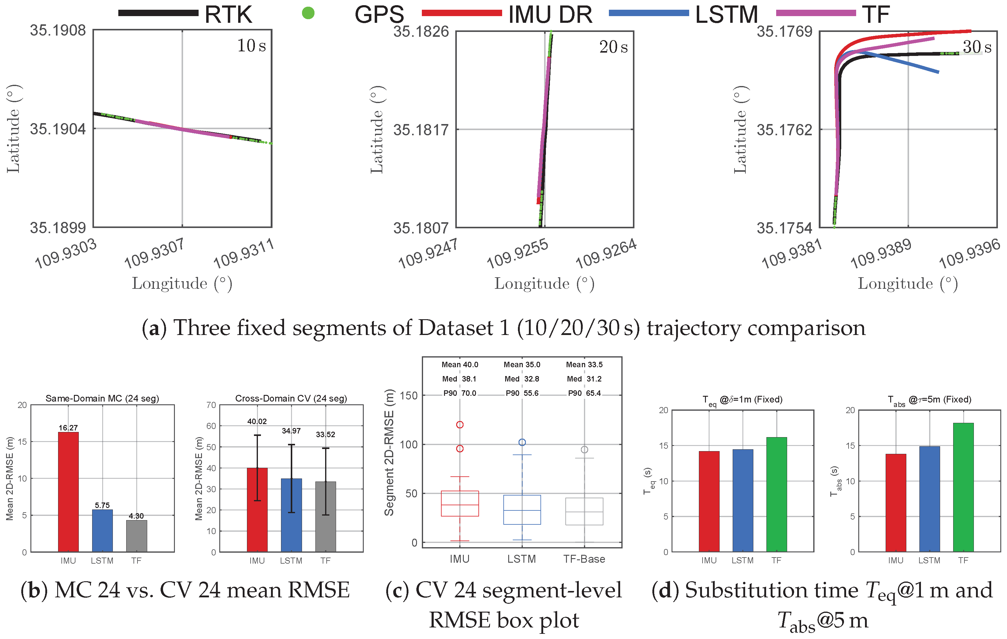
Same-domain basic performance and the cross-domain measure of true generalization differ markedly. On the three fixed outage segments of Dataset 1, pure IMU dead reckoning gives 2D-RMSE values of 5.88, 4.57, and 14.80 m for outage durations of 10, 20, and 30 s. TF-Base reduces these to 2.20, 2.42, and 6.63 m, and LSTM achieves comparable values. On the same-domain MC stress test of 24 segments, the mean RMSE drops from 16.27 m for IMU to 5.75 m for LSTM (64.7% improvement) and 4.30 m for TF-Base (73.6% improvement), so the neural networks compress the two-digit RMSE of pure IMU to a single digit. The complete summary appears in Table 6, with representative trajectories in Figure 8a and overall comparison in Figure 8b. The three fixed segments and the 24 MC segments of Dataset 1 lie on the same trajectory used for training, so the high improvement rates (73.6% for TF-Base and 64.7% for LSTM on MC) reflect the fitting quality on the training-aligned distribution rather than true generalization to unseen data. These same-domain numbers therefore cannot serve as the basis for comparing the algorithms.
The 24 CV segments of the independently collected Dataset 2, with no overlap with the training trajectory, give the true generalization measure: TF-Base reaches a mean RMSE of 33.52 m (16.3% improvement over pure IMU 40.02 m) and LSTM reaches 34.97 m (12.6% improvement). The two cross-domain improvements are close, as the right of Figure 8b shows, indicating that simply replacing the sequence backbone (LSTM versus Transformer) leaves no further room for capacity-driven gains on cross-domain data. The subsequent MGTR and TAMS evaluations therefore rely on the cross-domain 24-segment held-out set, and cross-domain metrics serve as the primary criterion of algorithm value.
TF-Base shows a clear tail risk trade-off in the cross-domain setting (Figure 8c,d): in the cross-domain, mean RMSE TF-Base (33.52 m) beats LSTM (34.97 m), but its P90 (65.41 m) is worse than LSTM’s (55.62 m, + 17.6 % ), and the substitution time T abs @ 5  m is 6.1 s for TF-Base versus 6.3 s for LSTM ( 3 % ). The GAP readout of TF-Base is competitive on the bulk distribution but locally unstable on cross-domain hard segments, directly motivating MGTR with tail-aware readout and motion gating.

4.3. Cross-Domain Evaluation and Complementarity of MGTR and TAMS

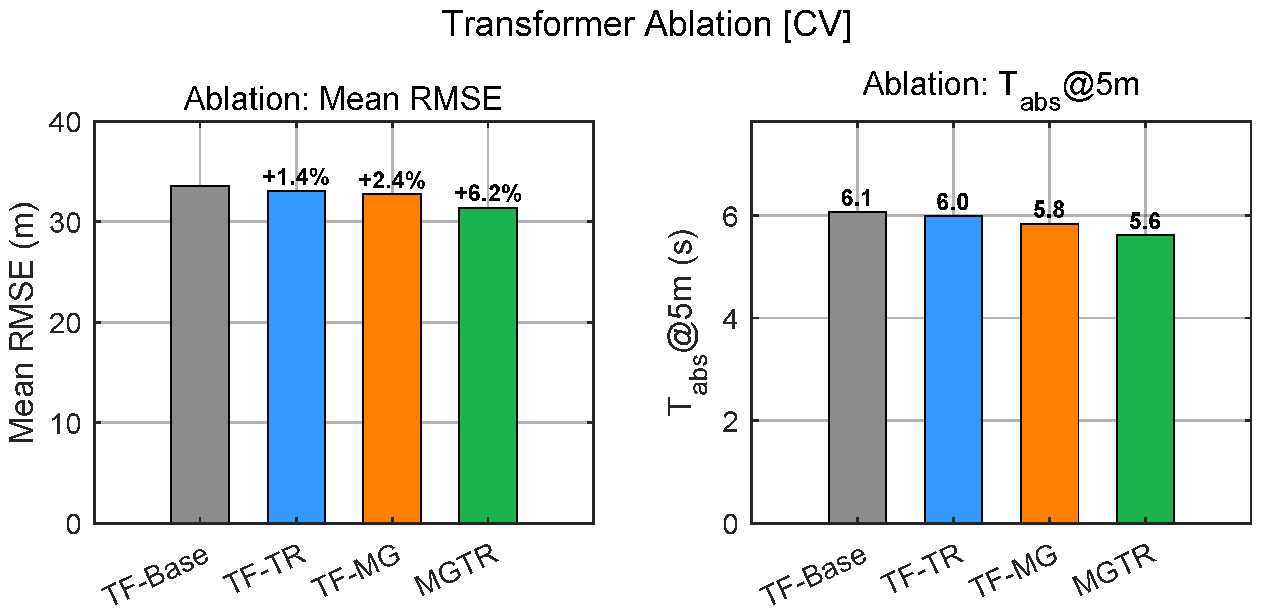
The cross-domain gain of MGTR has a tail-focused structure. On the 24 CV segments of Dataset 2, MGTR mean RMSE drops to 31.43 m, a 6.2% improvement over TF-Base 33.52 m (Table 7; Figure 9). Used alone, TF-TR improves the mean RMSE by 1.4% and TF-MG by 2.4%, so a simple additive estimate would give about 3.8%. The combined MGTR reaches 6.2%, well above this estimate, because hard segments often trigger the turning and the tail conditions at the same time. P90 drops from 65.41 m to 62.29 m (TF-TR, 4.8 % ), 54.65 m (TF-MG, 16.4 % ), and 52.12 m (MGTR, 20.3 % ), about three times the mean improvement. When TF-TR or TF-MG is used alone, the median RMSE rises slightly above TF-Base (33.40 and 34.48 vs. 31.21 m); only combined MGTR pulls the median back to 30.85 m while suppressing the tail.
Using P75 of TF-Base segment-level RMSE as a difficulty proxy, segments ≥P75 are hard (sox segments, one quarter; high-curvature turns, long accumulated drift, or low-speed start-up phases) and the rest are regular (18 segments). MGTR cuts hard-segment mean from 65.7 m to 54.8 m ( 10.9  m, 16.6 % ), while regular-segment mean barely changes (22.8 vs. 23.6 m). Almost all 6.2% gain comes from the ≥P75 segments.
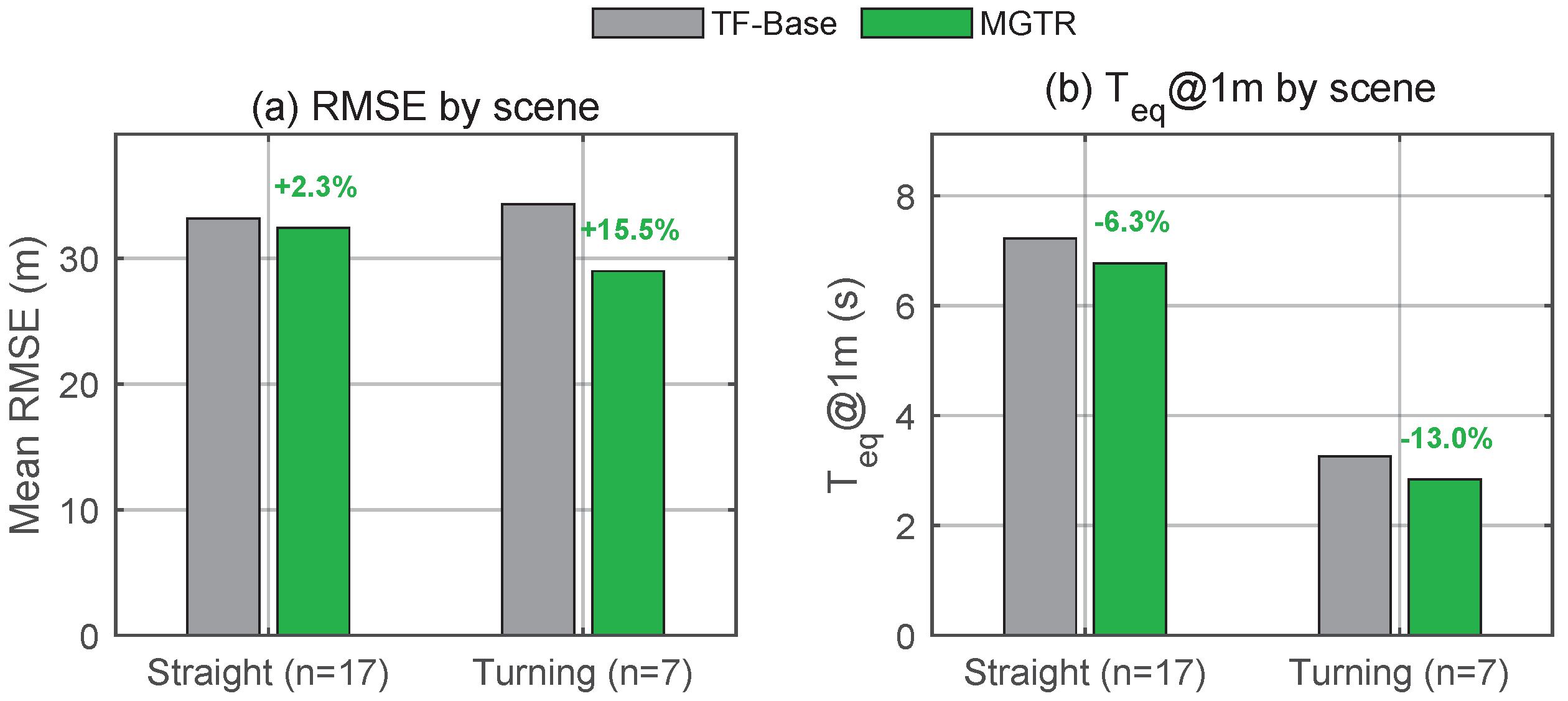
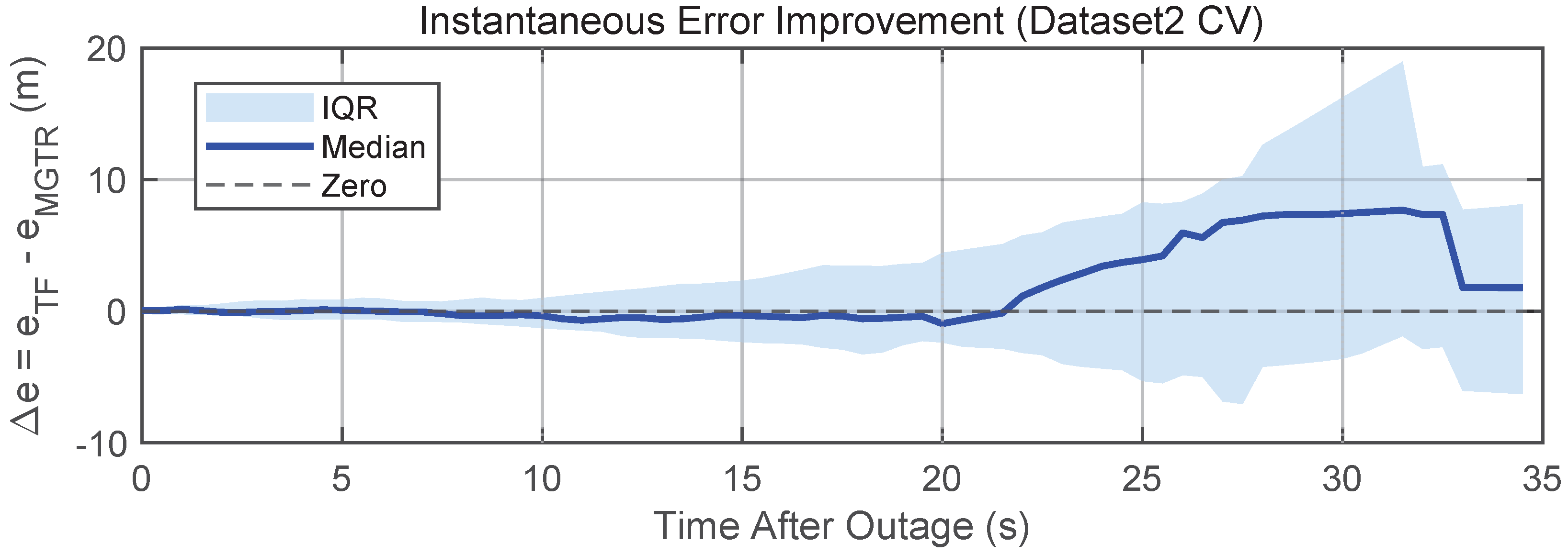
e ( t ) is roughly zero in the first 10 s; after ∼10 s its median becomes consistently positive, supporting a Delayed-Switch design that defers the second-stage choice to the late phase. The specific value T 0 = 6  s is then determined by the T 0 sweep on DS2-dev (Section 3.5, Figure 5). The MGTR gain comes almost entirely from turning segments (straight + 2.3 % vs. turning + 15.5 % ; Figure 10): the gating signal degenerates to near-identity on straight segments where ω z 0 .
TAMS robustness and the cost of the strict protocol are quantified next. Five independent runs select the representative model by mean RMSE on the three fixed validation segments of Dataset 1 (Run 3, validation RMSE 3.971 m); cross-domain results are reported afterwards. Cross-domain five-run statistics: mean RMSE 32.75 ± 1.33  m, median 31.23 ± 1.63  m, T abs @ 5  m 5.6 ± 0.6  s (coefficient of variation ∼4–5%); P90 reaches 61.04 ± 13.10  m (coefficient of variation 21%, peak 84.37 m on Run 5). The distribution is stable in the center and sensitive in the tail: softmax-sparse α t converges to different modes under different initializations. Run 4’s Dataset 2 mean RMSE is actually lower (31.14 vs. 31.73 m for Run 3), and the 0.59 m gap quantifies the cost of avoiding test set selection: had selection used Dataset 2 mean RMSE, TAMS improvement would rise from 5.3% to 7.1%.
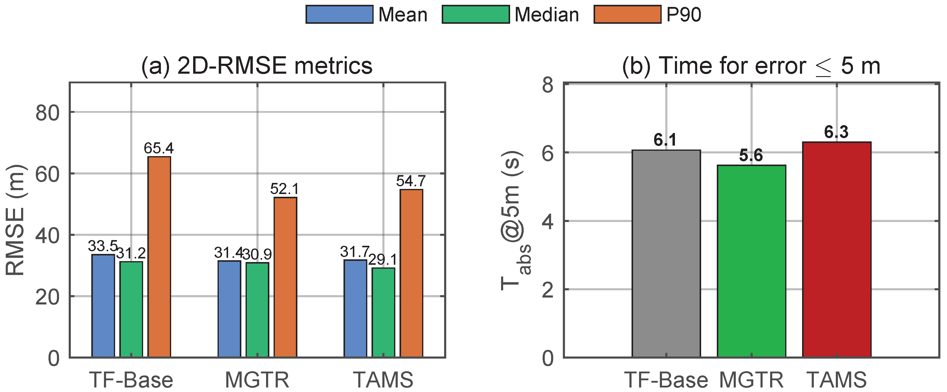
MGTR and TAMS exchange leadership across metrics on the cross-domain 24 segments (Figure 11): MGTR leads in mean RMSE and P90 (31.43 vs. 31.73 m and 52.12 vs. 54.73 m); TAMS leads in median RMSE and T abs @ 5  m (29.15 vs. 30.85 m and 6.3 vs. 5.6 s). The MGTR tail-aware readout ( K = 5 ) concentrates weight on the last steps and explicitly suppresses extreme tail risk; TAMS short-window mean pooling ( K = 10 ) is smoother and gives a longer continuously usable window on regular segments. The representative-segment time-series shows that TAMS is lower than MGTR in the first 10 s but rises faster afterwards. This binary choice between sustained availability and tail defense motivates restricting the Delayed-Switch pool to MGTR/TAMS and per-segment online selection. On the same-domain validation set, the TAMS mean RMSE of 3.971 m is on the same scale as TF-Base 3.75 m and serves only as a convergence reference.

4.4. Selection Strategy and Final Evaluation

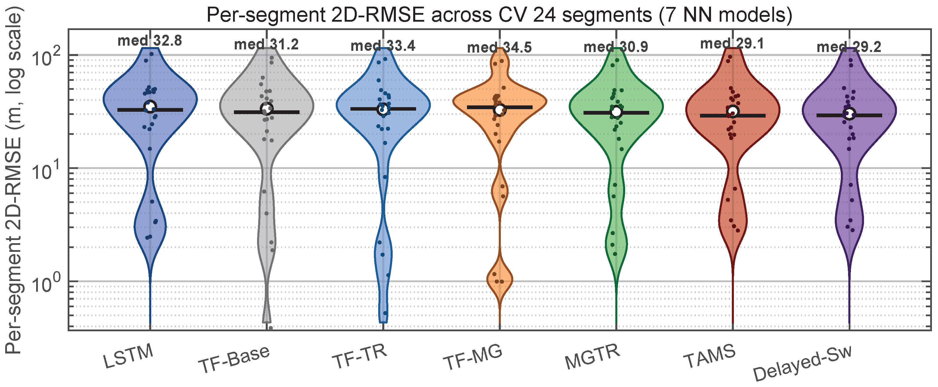
The segment-level 2D-RMSE on the 24 CV segments of Dataset 2 across the seven algorithms (IMU, LSTM, TF-Base, TF-TR, TF-MG, MGTR, TAMS) identifies the best model per segment. The per-segment winner distribution shows MGTR and TAMS each winning on six segments with almost disjoint winning sets, which is the direct basis for restricting the Delayed-Switch pool to MGTR/TAMS. TF-MG also wins on six segments but is dominated by MGTR in mean (31.43 vs. 32.71 m); its winning set is disjoint from MGTR’s, which suggests a possible three-way extension. TF-Base wins on four segments and IMU on two (the latter signals that training does not cover those two segments well); LSTM and TF-TR are dominated on all 24 segments. The neural-network mean RMSE values differ by only ∼2 m (TF-Base 33.52 vs. MGTR 31.43 m). The violin plus scatter view in Figure 12 explains the apparent paradox: distributions are nearly identical below ∼30 m, and the genuine difference concentrates in a handful of upper-tail hard segments, matching Section 4.3.
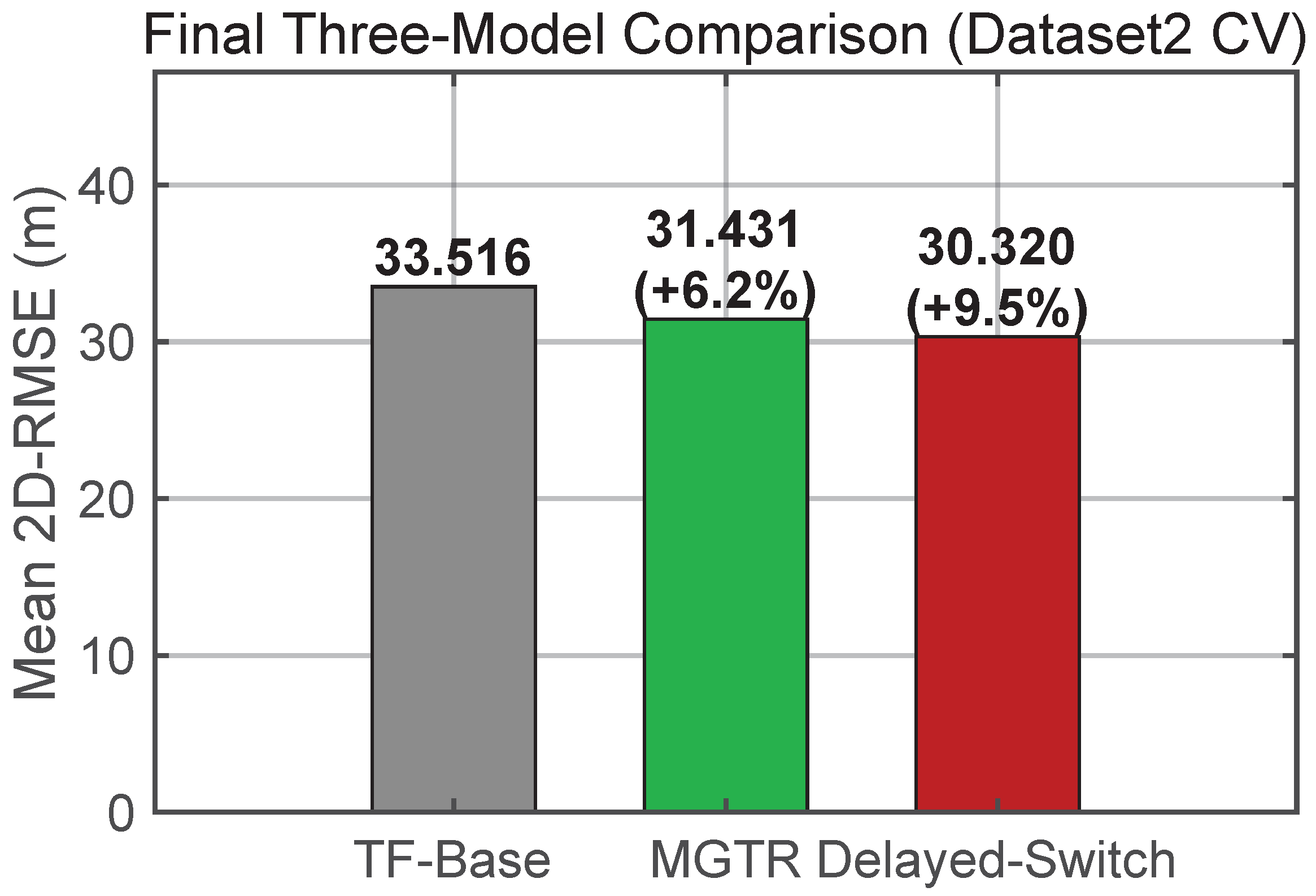
Delayed-Switch approaches the better-of-two oracle upper bound. Delayed-Switch fixes TF-Base for the first T 0 = 6  s and then uses a lasso classifier to select between MGTR and TAMS per segment. Its cross-domain mean RMSE is 30.32 m, 24.2 % vs. pure inertial dead reckoning (40.02 m), 9.5 % vs. TF-Base (33.52 m), 3.5 % vs. MGTR (31.43 m), and 4.4 % vs. TAMS (31.73 m). The single-model gains of MGTR and TAMS are 6.2% and 5.3%, while Delayed-Switch’s 9.5% reflects successful conditional selection. The oracle (TF-Base in stage one + per-segment hindsight pick from {MGTR, TAMS}) reaches 29.81 m, leaving Delayed-Switch only 0.51 m (∼1.7%) short. Figure 13 shows the lasso–oracle agreement via per-segment alignment and a 2 × 2 confusion matrix; disagreements concentrate on borderline segments where TF-Base RMSE is similar but MGTR/TAMS performance flips. Closing the remaining gap to the oracle requires extending the candidate pool (e.g., adding TF-MG for three-way selection) or adopting a non-linear classifier.
It should be noted that the Delayed-Switch lasso classifier is calibrated on DS2-dev (the development segments of Dataset 2 disjoint from the 24 held-out test segments) rather than evaluated in a fully zero-shot cross-domain setting. This models a realistic vehicle commissioning workflow where a brief one-pass calibration drive on the target deployment domain is operationally feasible, while the three backbones (TF-Base, MGTR, TAMS) remain unchanged.
The 6-vs-6 split of per-segment winners is not a statistical coincidence; it reflects a regime-based specialization that the lasso classifier learns from the development set. Among the six non-zero coefficients, S MT (net MGTR/TAMS displacement difference) and p 95 ( | g x | ) (lateral acceleration peak) tilt the decision toward MGTR, both of which mark turning-heavy segments where motion gating dominates. Conversely, ψ cum (net heading change) and v ¯ (mean speed) tilt toward TAMS, both of which mark sustained-motion segments where adaptive temporal aggregation outperforms a fixed motion prior. The classifier therefore separates segments along a turning-vs-sustained-drift axis.

Final Model Comparison

Table 8 summarizes the final metrics of TF-Base, MGTR, TAMS, and Delayed-Switch across three evaluation tiers: same-domain fixed segments, same-domain MC stress test, and cross-domain CV 24 segments. Delayed-Switch is trained and evaluated only on Dataset 2. On the cross-domain CV 24 segments, no single model dominates all four metrics (Table 8; Figure 14 for per-segment selection trajectory): Delayed-Switch gives the best mean RMSE at 30.32 m ( 24.2 % vs. pure inertial dead reckoning, 9.5 % vs. TF-Base), MGTR the best P90 at 52.12 m ( 20.3 % ), and TAMS the best median RMSE and T abs @ 5 m at 29.15 m and 6.3 s. TF-Base is last on every cross-domain metric.
Delayed-Switch’s four-metric ranks are 1, 2, 2, 2, the only configuration in the top two on every metric: median within 0.08 m of TAMS, P90 1.87 m above MGTR, T abs 0.1 s below TAMS. The explanation traces back to conditionally matching the inductive biases (Section 4.3, Figure 10).
The same-domain rows of Table 8 show the cost of these cross-domain mechanisms: MGTR degrades from 3.75 m (TF-Base) to 6.45 m on the three fixed DS1 segments and from 4.30 m to 5.14 m on the MC tier. Both components bias the model toward hard, turning-dominated patterns: the motion gate amplifies the encoder response whenever angular activity is present, and the tail readout gives up the smoothing of full-window averaging. On easy, training-aligned segments, the two mechanisms therefore over-correct trajectories that the GAP-based TF-Base already handles well. This trade-off is also why Delayed-Switch keeps TF-Base in the early phase and switches to the enhanced branches only when the segment calls for them.
Splitting by the P75 of TF-Base, the six hard segments gain 16.6% from MGTR while the 18 regular segments differ by only ∼0.8 m. The enhancement-module inductive biases match high-curvature or long-drift tails, while uniform GAP averaging suffices on regular segments—the direct rationale for Delayed-Switch keeping TF-Base on regular segments and switching to MGTR or TAMS on hard segments. Figure 15 visualizes the no-single-winner pattern in a four-panel bar chart.
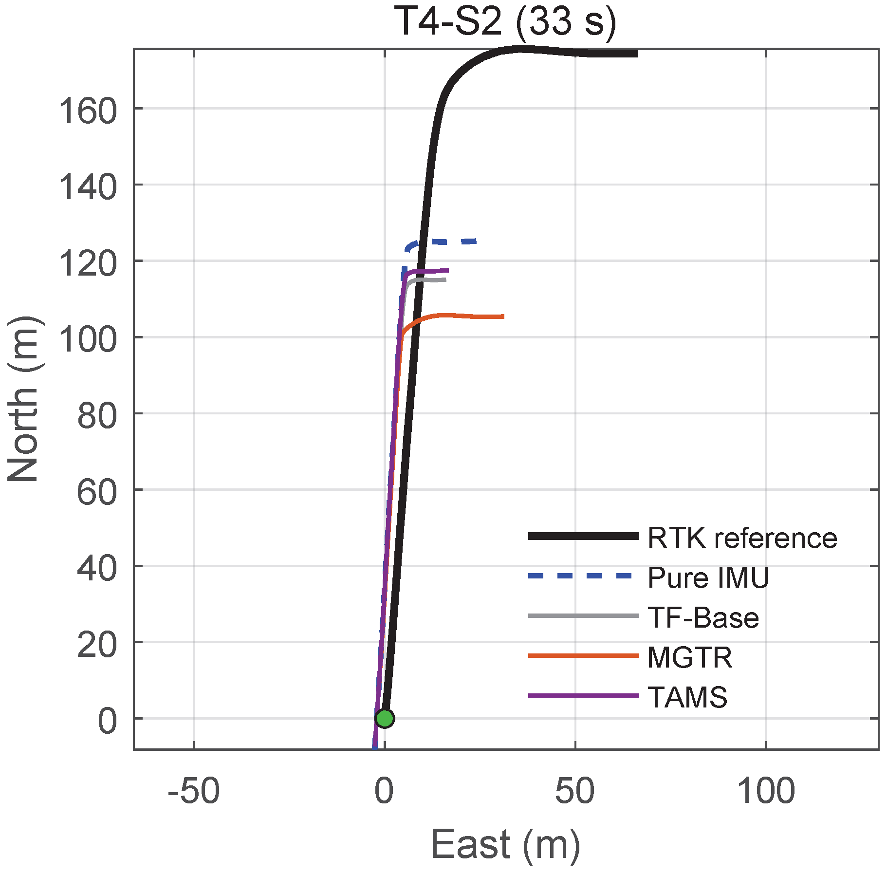
Table A1 in Appendix A also shows where the learned compensators fail. Pure IMU dead reckoning wins on two segments (segment identifiers Tn-Sm denote the held-out outage segments of Dataset 2 cataloged in Table A1). On T7-S3 (28 s), dead reckoning is nearly exact (1.49 m RMSE) because the segment is almost straight and the initial heading is well observed, so every learned correction only adds noise (3.97–7.11 m). On T4-S2 (33 s), all learned models over-correct (41.52–48.77 m versus 35.50 m for IMU; Figure 16), overshooting the reference more than uncorrected dead reckoning does. The abrupt maneuver segment T6-S2 (36 s) is hard for every method (83.67–102.04 m): once an early heading error forms under rapid maneuvering, none of the compensators recovers, and such segments dominate the residual P90 of all models. In short, IMU-sequence-based correction reduces drift on most outages and is counterproductive only at the extremes: it adds noise when dead reckoning is already accurate (T7-S3), and it overshoots when the correction exceeds what a hard segment needs (T4-S2) or when an abrupt maneuver defeats every method (T6-S2).

4.5. Comparison with Recent Learning-Based Baselines and Statistical Significance

For direct comparison with recent learning-based compensators, two representative baselines are reproduced under the identical protocol: AT-LSTM [21], which augments an LSTM with temporal attention, and CNN-GRU, the convolutional–recurrent design adopted by several recent outage-compensation systems [17,19,22]. The AT-LSTM implementation stacks a 64-unit LSTM, a learnable temporal attention pooling layer, and a two-layer regression head (FC(64), ReLU, FC(5)) (∼24K parameters); CNN-GRU stacks a causal 1-D convolution (kernel 3, 64 channels), a 64-unit GRU with last-step readout, and the same two-layer head (∼32K parameters). The causal padding guarantees that no future information enters the window, consistent with the online protocol of Section 3.2. Both baselines consume the same 12 dim. feature windows, the same 5 dim. labels, normalization, and loss, and the same zero-left-padded online inference and trajectory integration; each is trained three times and the representative run is selected by the Dataset 1 validation RMSE, exactly as for TAMS. Table 9 reports the cross-domain results next to the models of Table 8.
Two results are worth noting. First, both reproduced baselines have a higher cross-domain mean RMSE than the proposed models, though the gap is not always statistically significant. AT-LSTM reaches a 36.42 m mean RMSE, worse than the plain LSTM (34.97 m), so generic temporal attention by itself does not help with cross-domain drift; CNN-GRU reaches 32.70 m, statistically indistinguishable from TF-Base (Table 10). Second, CNN-GRU has the best same-domain validation RMSE of all compared models (2.96 m versus 3.75–3.97 m) but lands in the same cross-domain band as the other single predictors, which indicates that the bottleneck is the domain shift rather than in-domain fitting capacity. Once a reasonable backbone is in place, further cross-domain gains come from targeted mechanisms and from strategy-level selection, not from replacing the backbone with another generic sequence architecture.
Because the final test set contains 24 held-out segments and the differences among the top models are of the order of 1–3 m, formal paired statistics are reported in Table 10: two-sided Wilcoxon signed-rank tests on the per-segment 2D-RMSE pairs, Holm-corrected over the ten-comparison family, together with paired bootstrap 95% confidence intervals of the mean difference ( 10 4 resamples). Three conclusions follow. (i) Delayed-Switch is significantly better than AT-LSTM after Holm correction ( p raw = 0.0017 , p Holm = 0.017 ). (ii) The mean improvements of Delayed-Switch over TF-Base ( 3.20 m), TAMS ( 1.41 m), and CNN-GRU ( 2.38 m) have bootstrap intervals that exclude zero, although the rank tests do not reach significance at n = 24 : the improvement concentrates on the minority of hard segments while most segments are near-ties (median differences close to zero), consistent with Section 4.3, in particular, on segments where the selector picks a given branch the composite trajectory coincides with that branch after T 0 , which produces many near-zero paired differences and lowers the power of rank tests, whereas the bootstrap interval of the mean captures the concentrated tail gains. (iii) The backbone-level contrasts (TF-Base vs. LSTM, MGTR vs. TF-Base, TAMS vs. TF-Base, CNN-GRU vs. TF-Base) are all non-significant, which quantifies the earlier statement that replacing or augmenting the backbone alone yields limited cross-domain gains. No comparison shows Delayed-Switch significantly worse than any alternative.
Table 11 reports the computational cost of all compared models, measured on the experimental platform (MATLAB, single CPU thread). Every model holds within O ( 10 5 ) parameters and under 0.5 MB of FP32 weights, and the full per-step pipeline (window assembly, normalization, forward pass, and trajectory integration) runs at 2.9–7.1 ms per step, at least 28 times faster than the 0.2 s (5 Hz) sampling interval. In the worst-case Delayed-Switch phase, the three backbones run in parallel during the first T 0 and add one 18 dim. linear classification, totaling about 19.4 ms per step (with the three weight sets resident, ≈1.3 MB), still a tenfold real-time margin. The small footprint and per-step latency show that the models are lightweight and fast on the experimental platform. As these are desktop measurements (MATLAB, single CPU thread), they are not equivalent to execution on an automotive embedded processor, and the on-board latency and memory footprint would need a dedicated evaluation.

5. Conclusions

To address positioning drift during short GNSS outages on low-cost MEMS GNSS/IMU platforms, this paper proposes two targeted Transformer-based predictors and a lightweight inference-time fusion strategy. MGTR injects residual motion gating and a tail-aware readout into a Transformer baseline (TF-Base) to strengthen the response on hard segments and in the late stage of an outage. TAMS introduces learnable temporal attention pooling, short-window aggregation, and dual-head residual prediction to extract adaptive temporal features from non-stationary IMU sequences. Delayed-Switch retains TF-Base for the first 6 s of an outage and then selects between MGTR and TAMS per segment via a lasso classifier on 18 online features, without retraining any backbone; the classifier requires a one-pass calibration on a development split of the target domain, so the evaluation is not zero-shot. Evaluated under a three-tier protocol on two real-vehicle datasets where pure inertial dead reckoning yields a 40.02 m mean RMSE on cross-domain held-out segments, MGTR reduces the 90th-percentile 2D-RMSE by 20.3% over TF-Base, and Delayed-Switch reaches 30.32 m mean RMSE—a 24.2% reduction from pure inertial dead reckoning and a 9.5% reduction from TF-Base—within 0.51 m of the better-of-two upper bound. Under the identical protocol, Delayed-Switch also compares favorably with two recent learning-based baselines: the advantage over AT-LSTM is statistically significant after Holm correction, whereas the mean improvements over TF-Base, TAMS, and CNN-GRU have 95% bootstrap confidence intervals that exclude zero but do not reach statistical significance under the rank tests at this sample size (Section 4.5). The Delayed-Switch hybrid attains the lowest cross-domain mean RMSE among the four compared models and stays within the top two on every metric, with the gain concentrated on a minority of hard segments; this is consistent with explicit architectural enhancements and an inference-time selector addressing complementary failure modes of single-predictor compensators on low-cost vehicular platforms.
Several limitations should be noted. The study uses two datasets collected with one sensor suite in one city on two days, so geographic, seasonal, and sensor diversity is limited. The Delayed-Switch selector requires a one-pass calibration drive on the target domain and is therefore not zero-shot. The final test set contains 24 segments, which limits the statistical resolution of small differences among the top models—only the contrast against AT-LSTM survives multiple-comparison correction—and tail metrics such as P90 vary substantially across random seeds for every compared architecture (Appendix B). Absolute cross-domain errors remain large: on average, the prefix error exceeds 5 m after about 6 s ( T abs @ 5 m) and segment-level errors reach tens of meters (30.32 m mean), so during an outage, the system provides an approximate trajectory only. The proposed methods mitigate drift; they do not restore GNSS-level accuracy. Finally, several recent high-capacity architectures (e.g., FECAM-iTransformer and dual-domain networks [26,28]) were discussed but not reproduced because they target different sensor or sequence configurations. Beyond the tested durations (10–38 s), the absolute error grows roughly linearly with outage length: a dedicated evaluation of the frozen models at 40–120 s outages (Appendix F, Table A5) gives a mean segment-level 2D-RMSE that rises from 73.6 m at 40 s to 271.4 m at 120 s for pure dead reckoning and from 59.8 m to 186.5 m for MGTR. The proposed compensation reduces the error at all these durations, by a relative margin that increases with duration (MGTR improves on dead reckoning by 18.8% at 40 s and 31.3% at 120 s), but does not remove it. Extending the training data to longer outages and to more vehicles, cities, and sensor suites, testing a non-linear selector over a wider candidate pool, and integrating the compensators with filtering back ends remain future work. Because the present datasets record only the low-cost GNSS and IMU streams, fusing additional on-board sources that may remain available during an outage (wheel-speed odometry, steering angle, or map matching) could not be evaluated here and is left for future work; the first two relate directly to the speed and heading that dominate dead reckoning drift and could enter as extra input or gating channels, while map matching could serve as a road-network constraint at the fusion back end.

Author Contributions

Conceptualization, Z.L. (Ziyong Lei) and L.D.; methodology, Z.L. (Ziyong Lei) and L.D.; software, Z.L. (Ziyong Lei); validation, L.D.; formal analysis, Z.L. (Ziyong Lei); investigation, Z.L. (Ziyong Lei) and Z.L. (Zelong Lian); resources, Z.L. (Ziyong Lei), L.D., and Z.L. (Zelong Lian); data curation, Z.L. (Ziyong Lei) and Z.L. (Zelong Lian); writing—original draft preparation, Z.L. (Ziyong Lei); writing—review and editing, L.D.; visualization, Z.L. (Ziyong Lei); supervision, L.D.; project administration, L.D.; funding acquisition, L.D. All authors have read and agreed to the published version of the manuscript.

Funding

This research was funded by the Fundamental Research Funds for the Central Universities of China, grant numbers 104972026ZHZXhp0026 and 2025-ZDH-B1-01.

Institutional Review Board Statement

Not applicable.

Informed Consent Statement

Not applicable.

Data Availability Statement

The raw data supporting the conclusions of this article will be made available by the authors on request.

Conflicts of Interest

The authors declare no conflicts of interest.

Abbreviations

GNSSGlobal Navigation Satellite System
GPSGlobal Positioning System
IMUInertial Measurement Unit
ESKFError-State Kalman Filter
LSTMLong Short-Term Memory
TFTransformer
MGTRMotion-Guided Transformer with Tail-aware Readout
TAMSTemporal Attention Multi-Scale
RTKReal-Time Kinematic
DRDead Reckoning
GAPGlobal Average Pooling
ENUEast/North-Up
PEPositional Encoding

Appendix A. Cross-Domain Per-Segment 2D-RMSE Detail Table

Table A1 reports the segment-level 2D-RMSE on the 24 cross-domain CV segments of Dataset 2 for all seven algorithms (IMU, LSTM, TF-Base, TF-TR, TF-MG, MGTR, TAMS) and identifies the best model per segment. MGTR wins on six segments and TAMS wins on six segments, with almost disjoint winning sets—this is the empirical basis for restricting the Delayed-Switch second-stage candidate pool to MGTR/TAMS. TF-MG also wins on six segments but is dominated by MGTR on the mean (31.43 vs. 32.71 m); TF-Base wins on four and IMU on two (the latter signals that training does not cover those two segments well). LSTM and TF-TR are dominated on all 24 segments.
Table A1. Segment-level 2D-RMSE summary (m) of all algorithms on the 24 CV segments of Dataset 2 (corresponds to Section 4.4).
SegmentDurationSceneIMULSTMTF-BaseTF-TRTF-MGMGTRTAMSBest
T1-S136 s 120.0389.2885.8085.9588.5180.9788.35MGTR
T1-S220 s 29.5828.1127.8328.7929.8527.8125.46TAMS
T1-S326 s 14.563.326.218.345.645.633.06TAMS
T2-S127 s 37.7422.1121.1822.3224.0818.1421.97MGTR
T2-S232 s 43.9451.8863.1559.6642.5521.8419.73TAMS
T2-S332 s 60.3448.9155.1848.9551.4345.5950.99MGTR
T3-S127 s 34.0524.4626.7423.4627.1425.1422.88TAMS
T3-S217 s 1.622.481.881.131.002.103.46TF-MG
T3-S322 s 39.3528.9027.0630.7532.4828.1728.87TF-Base
T4-S133 s 57.2347.0639.1740.5741.0234.6643.75MGTR
T4-S233 s 35.5046.8543.2644.1143.6148.7741.52IMU
T4-S323 s 39.9533.1431.7935.4037.9233.5330.47TAMS
T5-S133 s 38.3845.6247.6736.7142.1041.5834.32TAMS
T5-S225 s 56.4449.3847.9745.9143.5748.9247.26TF-MG
T5-S326 s 30.9523.1017.5722.1420.0723.3718.45TF-Base
T6-S120 s 44.7137.9337.0637.1039.0935.6737.49MGTR
T6-S236 s 95.62102.0494.6192.0983.6789.9996.43TF-MG
T6-S326 s 48.2749.9941.2742.1439.4742.6343.02TF-MG
T7-S135 s 67.1646.6033.8134.1136.4738.6440.00TF-Base
T7-S220 s 3.792.422.212.201.151.742.81TF-MG
T7-S328 s 1.495.063.971.726.907.116.57IMU
T8-S135 s 2.263.420.390.520.992.665.25TF-Base
T8-S218 s 23.6614.8218.0016.7017.1614.7119.89MGTR
T8-S319 s 33.9032.3630.6232.6829.0834.9629.43TF-MG
Mean40.0234.9733.5233.0632.7131.4331.73
Median38.0632.7531.2133.4034.4830.8529.15
P9070.0055.6265.4162.2954.6552.1254.73

Appendix B. Robustness of the Compared Models Across Random Seeds

Table A2 reports the robustness of TAMS over five independent training runs. The representative model (Run 3, underlined) is selected on the Dataset 1 fixed validation segments; cross-domain results are reported only afterwards. Across the five runs, the cross-domain mean RMSE is 32.75 ± 1.33 m, with the tail (P90) showing larger variability ( 61.04 ± 13.10 m, coefficient of variation 21%), reflecting the sensitivity of the softmax-sparse temporal attention to random initialization. The central tendency (mean and median) is stable within ± 1.6 m across runs, justifying the use of validation set selection rather than cross-domain test set tuning.
Table A2. Robustness of TAMS over five independent training runs. The representative model is selected on the Dataset 1 validation set, and the Dataset 2 CV results are reported only afterwards. The underlined Run 3 is the representative model.
Training RunDS1 Val. RMSE (m)DS2 Mean RMSE (m)DS2 Median RMSE (m)DS2 P90 (m)DS2 T abs @ 5  m (s)
Run 14.68833.5332.7556.835.0
Run 24.91032.9230.2253.516.0
Run 33.97131.7329.1554.736.3
Run 45.26531.1431.0855.785.3
Run 55.72434.4332.9384.375.2
Mean ± std 4.91 ± 0.66 32.75 ± 1.33 31.23 ± 1.63 61.04 ± 13.10 5.6 ± 0.6
Following the same protocol, Table A3 reports three additional independent training runs each for TF-Base and MGTR, next to the fixed checkpoints used throughout the main text. Three observations follow. First, the central tendency varies across seeds with standard deviations of 0.7–2.4 m in the mean and 1.1–4.3 m in the median, comparable to the mean differences between the architectures themselves; this is consistent with the non-significant backbone-level contrasts of Section 4.5. Second, the tail is far more volatile than the center for every architecture (P90 standard deviations of 5.2–12.8 m here and 13.1 m for TAMS above), so single-checkpoint tail metrics should be read with caution. Third, the fixed checkpoints of the main text lie within (TF-Base) or near the favorable end of (MGTR) the observed ranges; since Delayed-Switch operates on these frozen checkpoints, the paired per-segment statistics of Section 4.5 are the right basis for the strategy-level claims, not a single-seed ranking of the architectures.
Table A3. Robustness of TF-Base and MGTR over three independent training runs each, under the protocol of Table A2. The “paper checkpoint” rows are the fixed models used in all main-text tables and by Delayed-Switch.
ModelTraining RunDS1 Val. RMSE (m)DS2 Mean RMSE (m)DS2 Median RMSE (m)DS2 P90 (m)DS2 T abs @ 5  m (s)
TF-BaseRun 14.10130.3627.1649.117.0
Run 26.38432.4932.7851.946.1
Run 36.04635.0435.4959.095.8
Mean ± std 32.63 ± 2.35 31.81 ± 4.25 53.38 ± 5.15 6.3 ± 0.6
Paper checkpoint3.7533.5231.2165.416.1
MGTRRun 15.70532.5231.2479.746.6
Run 26.43633.9532.9058.015.7
Run 34.73132.9433.2257.206.0
Mean ± std 33.13 ± 0.73 32.45 ± 1.06 64.98 ± 12.79 6.1 ± 0.5
Paper checkpoint6.4531.4330.8552.125.6

Appendix C. Per-Step Evidence for the Delayed-Switch Design and Hard-Segment Focus

The MGTR improvement over TF-Base admits two complementary decompositions of the same per-step squared error—one along the time axis (justifying the delayed switch) and one across segment difficulty (validating the hard-segment focus).
Time axis. Figure A1 shows the per-step improvement e ( t ) = e TF ( t ) e MGTR ( t ) over the 24 CV segments of Dataset 2. The median of e ( t ) is approximately zero during the first ∼10 s of an outage, then becomes consistently positive afterwards. This pattern provides the physical motivation for the Delayed-Switch design: in the early phase of an outage neither MGTR nor TAMS reliably outperforms TF-Base, so retaining TF-Base avoids unnecessary risk; the stable improvement after ∼10 s justifies the late-phase switch to MGTR/TAMS. The specific threshold T 0 = 6 s is then selected by the sweep in Section 3.5 (Figure 5).
Figure A1. Instantaneous error improvement e ( t ) = e TF ( t ) e MGTR ( t ) on the 24 CV segments of Dataset 2 (median and IQR). Positive values indicate MGTR outperforming TF-Base. The median curve is approximately zero in the first ∼10 s and becomes consistently positive afterwards.
Mathematics 14 02423 g0a1
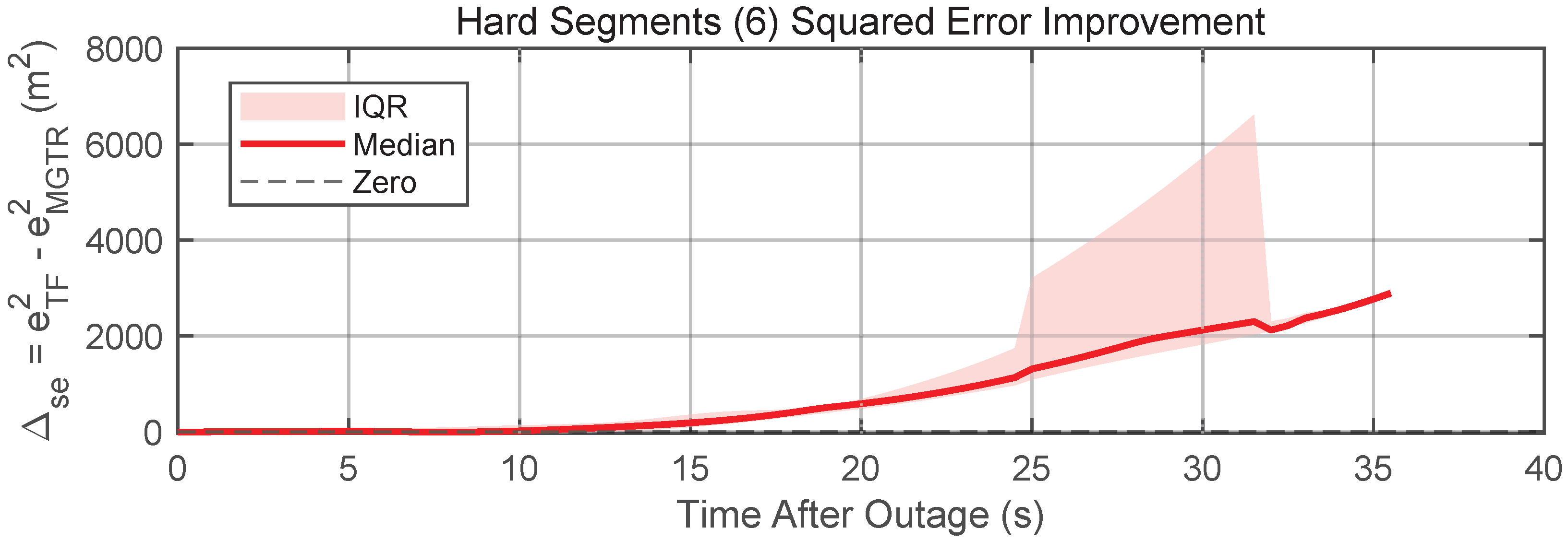
Segment axis. Figure A2 shows the squared error improvement s e ( t ) = e TF 2 ( t ) e MGTR 2 ( t ) on the six hard segments (upper P75 quartile of TF-Base RMSE) of the Dataset 2 CV 24 set. The median improvement grows steadily after ∼10 s, supporting the abstract claim that MGTR strengthens the hard-segment response; the 6.2% mean gain is concentrated on these segments where TF-Base struggles rather than spread uniformly across all 24 segments.
Figure A2. Squared error improvement s e ( t ) = e TF 2 ( t ) e MGTR 2 ( t ) on the six hard segments (upper P75 quartile of TF-Base RMSE) of the Dataset 2 CV 24 set (median and IQR). Positive values indicate MGTR outperforming TF-Base, with the gap widening after ∼15 s.
Mathematics 14 02423 g0a2

Appendix D. TF-Base Architecture Diagram

Figure A3 details the layer-level structure of the TF-Base encoder baseline configured in Section 3.2; it is placed here because the encoder follows the standard Transformer design.
Figure A3. Architecture of TF-Base, a Transformer encoder baseline for inertial drift correction. From left to right three processing stages are shown. The input and embedding stage concatenates 12 dim. IMU features with 8 dim. sinusoidal positional encoding and projects the 20 dim. augmented input to the 64 dim. hidden space. A stack of L = 2 encoder layers follows, each consisting of an MHSA sublayer and a position-wise FFN sublayer arranged in a Post-LN residual configuration. The readout stage applies global average pooling (GAP) over the time axis to obtain a 64 dim. global representation, which a linear head maps to a 5 dim. regression output. Dropout (0.1) is applied after the embedding and after each sublayer. Colors distinguish the functional blocks within the three stages, and the dashed outline and dashed connectors mark the zoomed-in detail of a single encoder layer and its scaled dot-product attention.
Mathematics 14 02423 g0a3

Appendix E. Hyperparameter Sensitivity

Table A4 reports a sensitivity analysis of the design hyperparameters. Each value follows from a design argument. The gating scale α = 0.5 keeps the gate multiplier 1 + α G in [ 1 , 1.5 ] , so the motion gate boosts an active step by at most 50% and never suppresses the backbone. The residual scale β = 0.1 keeps the TAMS auxiliary head a small correction to the main head. The readout windows K tail = 5 and K short = 10 cover the last 1 s and 2 s at 5 Hz, which capture the end of the outage where late drift concentrates and a recent-scale trend, respectively. The encoder is kept small ( L = 2 layers, h = 4 heads, d model = 64 ) because the input is short and low-dimensional. To test these choices, each hyperparameter is varied over a three-point grid with the others fixed, using one fixed-seed training run per setting on the 24 cross-domain segments. Across all eighteen settings the cross-domain mean RMSE stays within 31.0–35.3 m, always far below pure dead reckoning (40.02 m) and close to or below TF-Base (33.52 m), so no choice in these ranges breaks the method. The error also grows where each argument predicts: an over-large gate ( α = 0.7 ) over-amplifies the encoder output; an over-long tail window ( K tail = 10 ) blurs the focus on the outage end and raises the P90 to 82.98 m; and eight attention heads over-parameterize the short input and raise the P90 to 87.00 m. The default values sit at the favorable end of every range.
Table A4. Hyperparameter sensitivity on the cross-domain evaluation (Dataset 2 CV 24 segments). Each hyperparameter is varied over a three-point grid around its default (marked *), with all other hyperparameters held at their defaults and one fixed-seed training run per setting. The gating scale α , tail window K tail , attention heads, and encoder layers are varied on MGTR; the residual scale β and short window K short on TAMS.
HyperparameterValueMean RMSE (m)Median (m)P90 (m) T abs @ 5  m (s)
α (MGTR gating)0.331.9431.4052.545.9
0.5 *31.8531.0052.626.8
0.733.5833.4956.285.3
K tail (MGTR readout)333.7232.7558.995.7
5 *31.8531.0052.626.8
1034.0430.0682.986.6
Attention heads232.9631.0057.766.3
4 *31.8531.0052.626.8
835.2833.3087.005.7
Encoder layers133.0333.0455.716.0
2 *31.8531.0052.626.8
333.6932.9959.365.8
β (TAMS residual)0.0532.6931.6958.726.1
0.1 *31.0230.0551.785.8
0.233.6632.6663.415.5
K short (TAMS)534.1932.9164.606.1
10 *31.0230.0551.785.8
1533.9332.8263.475.8

Appendix F. Robustness to Longer Outages

To assess behavior beyond the tested durations, the frozen models were evaluated on Dataset 2 outages of 40–120 s—well outside the 10–40 s training range—with no retraining, using the same mean segment-level 2D-RMSE over 13 segments per duration (Table A5). The absolute error grows with outage length, from 73.6 m at 40 s to 271.4 m at 120 s for pure dead reckoning and from 59.8 m to 186.5 m for MGTR. Across all durations the learned compensators are more accurate than pure dead reckoning, by a relative margin that increases with duration: MGTR improves on dead reckoning by 18.8% at 40 s and by 31.3% at 120 s. The last column is the per-segment better-of-MGTR/TAMS oracle bound that Delayed-Switch targets.
Table A5. Robustness to longer GNSS outages on Dataset 2 (mean segment-level 2D-RMSE, m; frozen models, no retraining; 13 segments per duration). The last column is the per-segment better-of-MGTR/TAMS oracle bound approached by Delayed-Switch.
Outage (s)IMU (DR)TF-BaseMGTRTAMSBetter-of-MGTR/TAMS
4073.5961.3759.7762.4958.95
60130.90110.28105.01109.48103.14
80181.50151.75139.64147.40137.09
100226.98188.42163.46179.04162.08
120271.43224.89186.49211.91185.98

References

  1. Huang, Y.; Zhu, B.; Zhao, J.; Han, J.; Song, D.; Zhang, P.; Jia, S.; Gao, M. Criticality Assessment Model for Intelligent Vehicle Test Scenario Based on Interactive Field Feature and Hypergraph Learning. IEEE Trans. Intell. Transp. Syst. 2026, 27, 4125–4139. [Google Scholar] [CrossRef]
  2. Dong, Y.; Wang, D.; Zhang, L.; Li, Q.; Wu, J. Tightly Coupled GNSS/INS Integration with Robust Sequential Kalman Filter for Accurate Vehicular Navigation. Sensors 2020, 20, 561. [Google Scholar] [CrossRef]
  3. Liu, J.; Guo, G. Vehicle Localization During GPS Outages With Extended Kalman Filter and Deep Learning. IEEE Trans. Instrum. Meas. 2021, 70, 7503410. [Google Scholar] [CrossRef]
  4. Lee, W.; Cho, H.; Hyeong, S.; Chung, W. Practical Modeling of GNSS for Autonomous Vehicles in Urban Environments. Sensors 2019, 19, 4236. [Google Scholar] [CrossRef] [PubMed]
  5. Jwo, D.-J.; Biswal, A.; Mir, I.A. Artificial Neural Networks for Navigation Systems: A Review of Recent Research. Appl. Sci. 2023, 13, 4475. [Google Scholar] [CrossRef]
  6. Gu, Y.; Hsu, L.-T.; Kamijo, S. Passive Sensor Integration for Vehicle Self-Localization in Urban Traffic Environment. Sensors 2015, 15, 30199–30220. [Google Scholar] [CrossRef] [PubMed]
  7. Lim, J.; Yoo, W.J.; Kim, L.W.; Lee, Y.D.; Lee, H.K. Augmentation of GNSS by Low-Cost MEMS IMU, OBD-II, and Digital Altimeter for Improved Positioning in Urban Area. Sensors 2018, 18, 3830. [Google Scholar] [CrossRef] [PubMed]
  8. Sun, R.; Yang, Y.; Chiang, K.-W.; Duong, T.-T.; Lin, K.-Y.; Tsai, G.-J. Robust IMU/GPS/VO Integration for Vehicle Navigation in GNSS Degraded Urban Areas. IEEE Sens. J. 2020, 20, 10110–10122. [Google Scholar] [CrossRef]
  9. Groves, P.D.; Wang, L.; Walter, D.; Martin, H.; Voutsis, K.; Jiang, Z. The Four Key Challenges of Advanced Multisensor Navigation and Positioning. In Proceedings of the 2014 IEEE/ION Position, Location and Navigation Symposium (PLANS 2014), Monterey, CA, USA, 5–8 May 2014; IEEE: Piscataway, NJ, USA, 2014; pp. 773–792. [Google Scholar] [CrossRef]
  10. Gao, J.; Li, K.; Chen, J. Research on the Integrated Navigation Technology of SINS with Couple Odometers for Land Vehicles. Sensors 2020, 20, 546. [Google Scholar] [CrossRef] [PubMed]
  11. Wang, Z.; Li, B.; Dan, Z.; Wang, H.; Fang, K. 3D LiDAR Aided GNSS/INS Integration Fault Detection, Localization and Integrity Assessment in Urban Canyons. Remote Sens. 2022, 14, 4641. [Google Scholar] [CrossRef]
  12. Niu, X.; Tang, H.; Zhang, T.; Fan, J.; Liu, J. IC-GVINS: A Robust, Real-Time, INS-Centric GNSS-Visual-Inertial Navigation System. IEEE Robot. Autom. Lett. 2023, 8, 216–223. [Google Scholar] [CrossRef]
  13. Li, J.; Sun, R.; Wang, Y.; Ochieng, W.Y. A Robust Time Synchronization Algorithm for GNSS/IMU Integrated Navigation in Urban Environments. Meas. Sci. Technol. 2025, 36, 036302. [Google Scholar] [CrossRef]
  14. Sun, R.; Sheng, Q.; Cheng, Q.; Shang, X.; Ochieng, W.Y. 3-D Grid-Based Resilient Pseudorange Error Prediction for Adaptive GNSS/IMU Integrated Navigation in Urban Areas. IEEE Internet Things J. 2025, 12, 19264–19279. [Google Scholar] [CrossRef]
  15. Zhi, Z.; Liu, D.; Liu, L. A Performance Compensation Method for GPS/INS Integrated Navigation System Based on CNN–LSTM during GPS Outages. Measurement 2022, 188, 110516. [Google Scholar] [CrossRef]
  16. Tang, Y.; Jiang, J.; Liu, J.; Yan, P.; Tao, Y.; Liu, J. A GRU and AKF-Based Hybrid Algorithm for Improving INS/GNSS Navigation Accuracy during GNSS Outage. Remote Sens. 2022, 14, 752. [Google Scholar] [CrossRef]
  17. Zhao, S.; Zhou, Y.; Huang, T. A Novel Method for AI-Assisted INS/GNSS Navigation System Based on CNN-GRU and CKF during GNSS Outage. Remote Sens. 2022, 14, 4494. [Google Scholar] [CrossRef]
  18. Liu, F.; Zhao, H.; Chen, W. A Hybrid Algorithm of LSTM and Factor Graph for Improving Combined GNSS/INS Positioning Accuracy during GNSS Interruptions. Sensors 2024, 24, 5605. [Google Scholar] [CrossRef] [PubMed]
  19. Zhao, H.; Liu, F.; Chen, W. A Method for Assisting GNSS/INS Integrated Navigation System during GNSS Outage Based on CNN-GRU and Factor Graph. Appl. Sci. 2024, 14, 8131. [Google Scholar] [CrossRef]
  20. Wang, Y.; Wang, Q.; Zhang, H.; Duan, X. A Low-Cost GNSS/INS Integration Method Aided by Cascade-LSTM Pseudo-Velocity Measurement for Bridging GNSS Outages. Measurement 2025, 240, 115518. [Google Scholar] [CrossRef]
  21. Chen, S.; Xin, M.; Yang, F.; Zhang, X.; Liu, J.; Ren, G.; Kong, S. Error Compensation Method of GNSS/INS Integrated Navigation System Based on AT-LSTM During GNSS Outages. IEEE Sens. J. 2024, 24, 20188–20199. [Google Scholar] [CrossRef]
  22. Meng, X.; Tan, H.; Yan, P.; Zheng, Q.; Chen, G.; Jiang, J. A GNSS/INS Integrated Navigation Compensation Method Based on CNN-GRU + IRAKF Hybrid Model During GNSS Outages. IEEE Trans. Instrum. Meas. 2024, 73, 2510015. [Google Scholar] [CrossRef]
  23. Zhang, H.; Xiong, H.; Hao, S.; Yang, G.; Wang, M.; Chen, Q. A Novel Multidimensional Hybrid Position Compensation Method for INS/GPS Integrated Navigation Systems During GPS Outages. IEEE Sens. J. 2024, 24, 962–974. [Google Scholar] [CrossRef]
  24. Liu, Y.; Hu, T.; Zhang, H.; Wu, H.; Wang, S.; Ma, L.; Long, M. iTransformer: Inverted Transformers Are Effective for Time Series Forecasting. In Proceedings of the Twelfth International Conference on Learning Representations (ICLR 2024); OpenReview.net: Alameda, CA, USA, 2024; Available online: https://openreview.net/forum?id=JePfAI8fah (accessed on 28 June 2026).
  25. Wang, H.; Tang, F.; Wei, J.; Zhu, B.; Wang, Y.; Zhang, K. Online Semi-Supervised Transformer for Resilient Vehicle GNSS/INS Navigation. IEEE Trans. Veh. Technol. 2024, 73, 16295–16311. [Google Scholar] [CrossRef]
  26. Kuang, X.; Yan, B. A Novel FECAM-iTransformer Algorithm for Assisting INS/GNSS Navigation System during GNSS Outages. Appl. Sci. 2024, 14, 8753. [Google Scholar] [CrossRef]
  27. Guyard, K.C.; Bertolaccini, J.; Montavon, S.; Deriaz, M. A Transformer Encoder Approach for Localization Reconstruction During GPS Outages from an IMU and GPS-Based Sensor. Sensors 2025, 25, 522. [Google Scholar] [CrossRef] [PubMed]
  28. Wang, Z.; Wang, J.; Hou, X.; Guo, J.; Fang, K.; Huang, X.; Sun, R.; Song, D. A Robust and Adaptive Framework for GNSS/INS Integrated Navigation Based on Dual-Domain Deep Learning Network during GNSS Outages. Chin. J. Aeronaut. 2026, in press. [Google Scholar] [CrossRef]
  29. Sharaf, R.; Noureldin, A.; Osman, A.; El-Sheimy, N. Online INS/GPS Integration with Radial Basis Function Neural Networks. IEEE Aerosp. Electron. Syst. Mag. 2005, 20, 8–14. [Google Scholar] [CrossRef]
  30. Tan, X.; Wang, J.; Jin, S.; Meng, X. GA-SVR and Pseudo-Position-Aided GPS/INS Integration During GPS Outage. J. Navig. 2015, 68, 678–696. [Google Scholar] [CrossRef]
  31. Yao, Y.; Xu, X.; Zhu, C.; Chan, C.-Y. A Hybrid Fusion Algorithm for GPS/INS Integration During GPS Outages. Measurement 2017, 103, 42–51. [Google Scholar] [CrossRef]
  32. Shen, C.; Zhang, Y.; Tang, J.; Cao, H.; Liu, J. Dual-Optimization for a MEMS-INS/GPS System During GPS Outages Based on the Cubature Kalman Filter and Neural Networks. Mech. Syst. Signal Process. 2019, 133, 106222. [Google Scholar] [CrossRef]
  33. Hochreiter, S.; Schmidhuber, J. Long Short-Term Memory. Neural Comput. 1997, 9, 1735–1780. [Google Scholar] [CrossRef] [PubMed]
  34. Fang, W.; Jiang, J.; Lu, S.; Gong, Y.; Tao, Y.; Tang, Y.; Yan, P.; Luo, H.; Liu, Z. A LSTM Algorithm Estimating Pseudo Measurements for Aiding INS During GNSS Signal Outages. Remote Sens. 2020, 12, 256. [Google Scholar] [CrossRef]
  35. Dellaert, F.; Kaess, M. Factor Graphs for Robot Perception. Found. Trends Robot. 2017, 6, 1–139. [Google Scholar] [CrossRef]
  36. Zhang, H.; Wang, Y.; Shan, S.; Wang, Q.; Li, M.; Han, F.; Duan, X. An Enhanced GNSS/INS Navigation Compensation Method Using LSTM-FPN for Bridging GNSS Outages. Meas. Sci. Technol. 2025, 36, 016339. [Google Scholar] [CrossRef]
  37. Gao, W.; Feng, Y. Assessing the Robustness of Machine Learning Strategy for GNSS/INS Vehicle Positioning Solutions Enhancement. GPS Solut. 2025, 29, 167. [Google Scholar] [CrossRef]
  38. Li, X.; Wang, X.; Pei, C. Handling Method for GPS Outages Based on PSO-LSTM and Fading Adaptive Kalman Filtering. Sci. Rep. 2025, 15, 11817. [Google Scholar] [CrossRef] [PubMed]
  39. Guo, Y.; Sun, Y.; Zhuang, G.; Zhou, D. A Robust Navigation Algorithm Without GNSS Based on Deep Learning and Variational Bayesian Filter. Meas. Sci. Technol. 2025, 36, 036310. [Google Scholar] [CrossRef]
  40. Vaswani, A.; Shazeer, N.; Parmar, N.; Uszkoreit, J.; Jones, L.; Gomez, A.N.; Kaiser, Ł.; Polosukhin, I. Attention Is All You Need. In Advances in Neural Information Processing Systems 30 (NeurIPS 2017); Curran Associates, Inc.: Long Beach, CA, USA, 2017; pp. 5998–6008. Available online: https://papers.neurips.cc/paper/7181-attention-is-all-you-need (accessed on 28 June 2026).
  41. Liu, Z.; Guan, L.; Wang, X.; Sun, H.; Karaim, M.; Gao, Y. CNN–Transformer-Enhanced GNSS/RISS Integrated Navigation Algorithm Based on RISS Recomputed Method. Electronics 2026, 15, 2040. [Google Scholar] [CrossRef]
  42. Solà, J. Quaternion Kinematics for the Error-State Kalman Filter. arXiv 2017, arXiv:1711.02508. [Google Scholar] [CrossRef]
  43. Tibshirani, R. Regression Shrinkage and Selection via the Lasso. J. R. Stat. Soc. Ser. B 1996, 58, 267–288. [Google Scholar] [CrossRef]
Figure 1. End-to-end pipeline of the proposed framework. ESKF fusion feeds GNSS-aided positioning during availability and falls back to heading-constrained IMU dead reckoning at outage; the resulting feature window drives four sequence models (LSTM, TF-Base, MGTR, TAMS), and the Delayed-Switch strategy layer selects per-segment between TF-Base in the first T 0 = 6 s and MGTR/TAMS afterwards.
Mathematics 14 02423 g001
Figure 2. Architecture of MGTR, a Motion-Guided Transformer with Tail-aware Readout. The top row shows the end-to-end data flow: MGTR inherits the input and embedding and the L = 2 Post-LN Transformer encoder stack from TF-Base (blue-shaded), and inserts two enhancement modules between the encoder and the regression head, replacing the GAP readout. The bottom-left panel details TF-MG, a residual motion-guided gating module: three motion channels, namely the gyroscope z-axis angular rate ω z , the cumulative heading change, and the dead reckoning speed v DR , feed a two-layer MLP (FC, ReLU, FC, sigmoid) that produces a per-step gating signal G ( 0 , 1 ) T . The encoder output is modulated by H out = H ( 1 + α · G ) with α = 0.5 , so that G approaches 1 on dynamic steps and 0 on smooth steps, where the latter degenerates to an identity-like mapping H out H . The bottom-right panel details TF-TR, a tail-aware readout that concatenates the last time step h T with the average of the last K = 5 steps h ¯ tail , replacing the global average pooling of TF-Base to emphasize the most recent motion state during late-outage phases. In the figure, blue, green, and purple boxes mark components inherited from TF-Base, TF-MG-specific components, and TF-TR-specific components, respectively; in the gating illustration, green and red squares denote high and low per-step gating values on dynamic (turning) and smooth (straight) steps.
Mathematics 14 02423 g002
Figure 3. Architecture of TAMS for inertial drift correction. TAMS inherits the input and embedding and the L = 2 Post-LN Transformer encoder stack from TF-Base (blue-shaded). After the encoder produces H = [ h 1 , , h T ] R d model × T , three mechanisms redesign the readout and prediction stages. Temporal attention pooling computes softmax weights α t = exp ( w h t ) / j exp ( w h j ) via a single learnable projection vector w R d model , intentionally not MHSA in order to limit readout parameters, and aggregates a global representation h attn . Short-window mean pooling averages the last K = 10 steps (the most recent 2 s at 5 Hz) into h short , a recent-scale branch complementary to the global attention pooling. The two are concatenated into a 2 d model = 128 dim. dual-scale representation [ h attn ; h short ] and fed into dual-head residual prediction: the main head FC ( d model ) , ReLU, FC ( 5 ) produces y ^ main that fits the dominant drift trend, while the residual head FC ( d model / 2 ) , ReLU, FC ( 5 ) produces y ^ res , which is scaled by β = 0.1 and added to obtain y ^ = y ^ main + β · y ^ res R 5 . The bottom Adaptive Attention Insight panel illustrates the learned adaptive behavior of α t : tail-focused on dynamic segments such as turns or accelerations and near-uniform on steady paths. In the figure, blue, purple, and green boxes mark components inherited from TF-Base, TAMS-specific components, and the short-window mean-pooling branch, respectively; the circled plus denotes the residual summation, and the colored cells in the Adaptive Attention Insight panel depict the learned per-step attention weights α t .
Mathematics 14 02423 g003
Figure 4. Three-panel structure of the Delayed-Switch inference-time strategy. The main panel illustrates the parallel inference of TF-Base, MGTR, and TAMS together with the switching decision, where the first stage [ 0 , T 0 ] is fixed to TF-Base and the second stage chooses between MGTR and TAMS via the lasso classifier f with threshold τ = 0.95 . The lower panel illustrates the two-stage offline determination procedure. The right panel lists the lasso non-zero features and the decision rule. See Section 3.5 for details.
Mathematics 14 02423 g004
Figure 5. Stage-one selection of T 0 on DS2-dev: the oracle-guided upper bound is swept over T 0 { 6 , 7 , , 16 } s. (a) Mean 2D-RMSE. (b) Mean T abs @ 5 m. The three curves correspond to fixing the second stage to MGTR, fixing it to TAMS, and selecting per segment by the oracle. The vertical dashed line marks the selected T 0 = 6 s.
Mathematics 14 02423 g005
Figure 6. Lasso coefficients of the 18 online features for the Delayed-Switch classifier (trained after z-score normalization, ranked top to bottom by | β | ). Bars to the right (positive) favor TAMS while bars to the left (negative) favor MGTR. After lasso sparsification, only six dimensions are non-zero and twelve are shrunk to zero. The sign stability and the mechanistic interpretation appear in the main text.
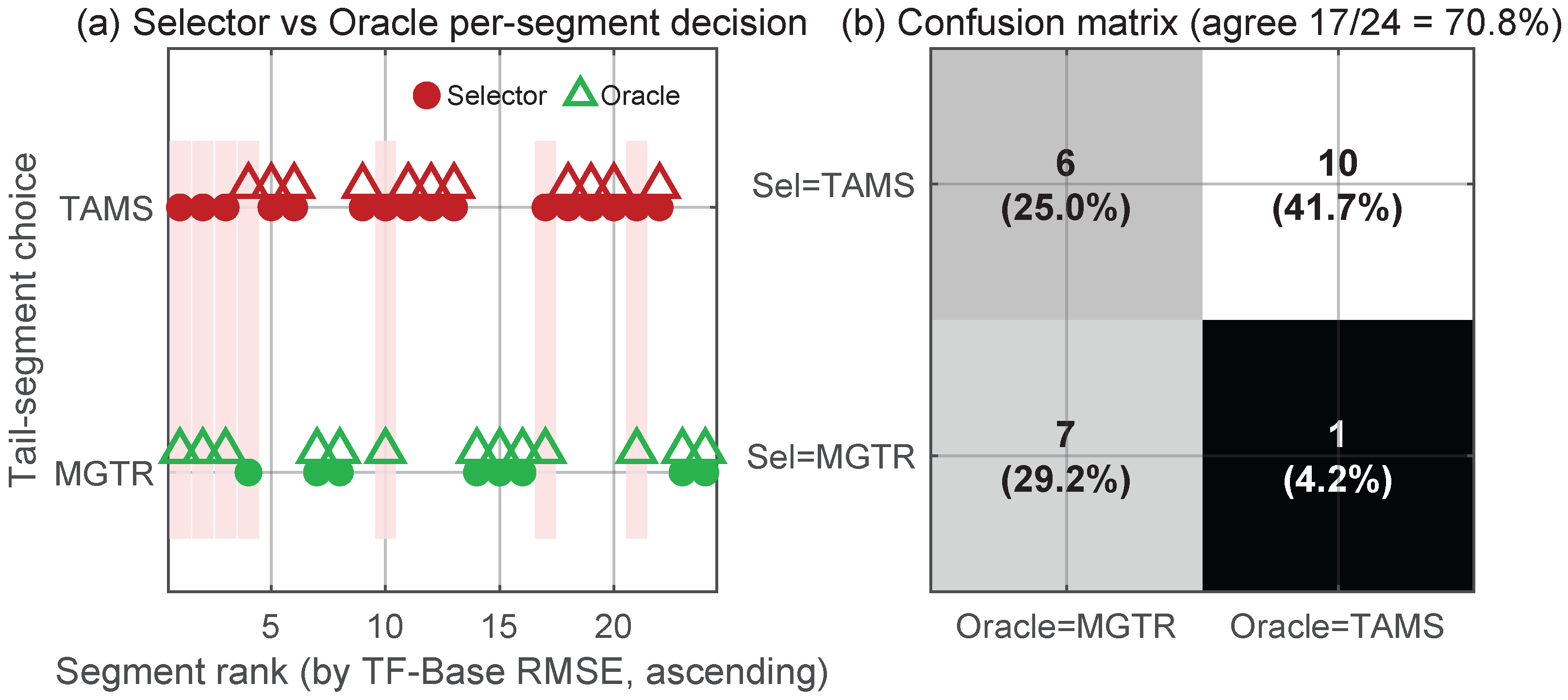
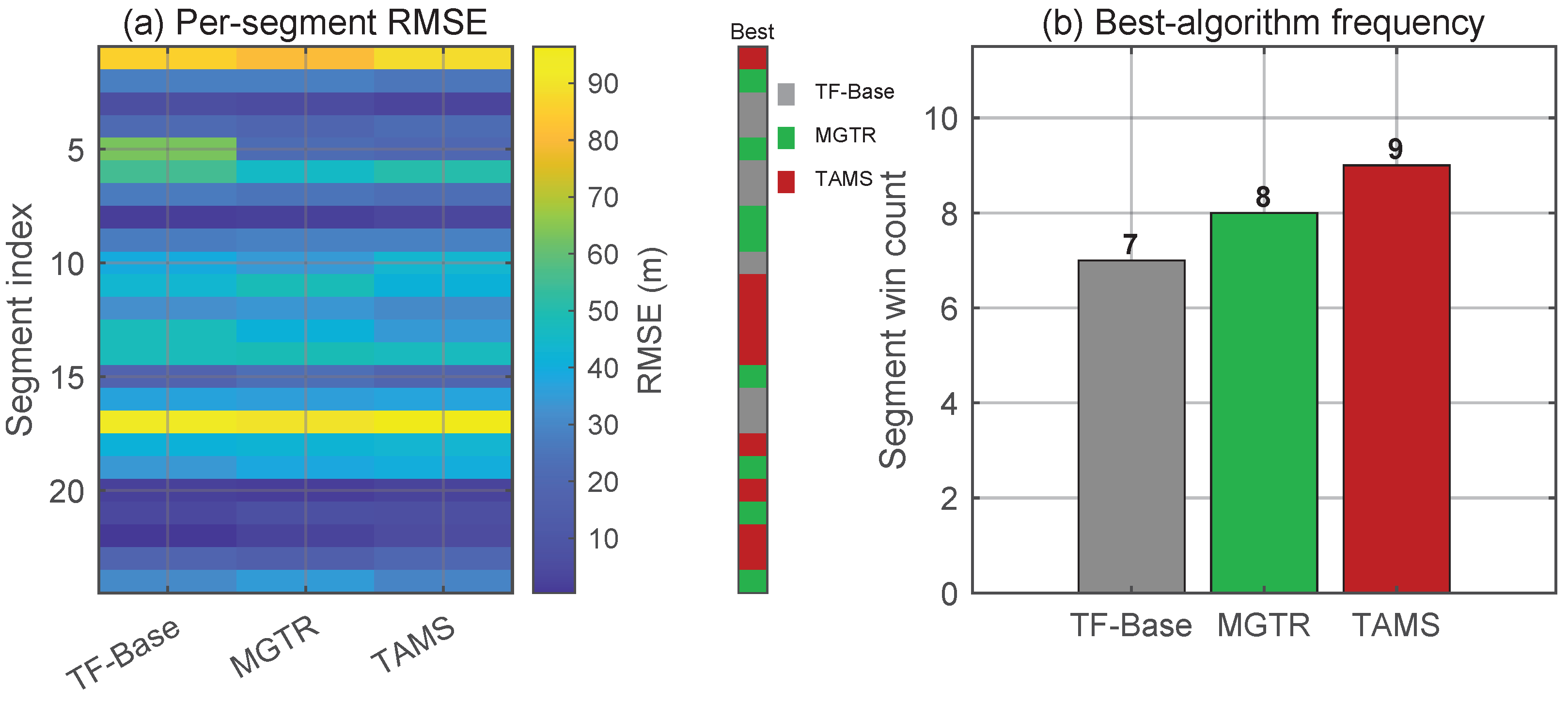
Mathematics 14 02423 g006
Figure 7. Collection overviews of the two real-vehicle datasets in geographic coordinates on a satellite basemap. (a) Dataset 1: full GPS measured track and RTK reference. (b) Dataset 2: subsampled GPS fixes and RTK reference trajectory.
Mathematics 14 02423 g007
Figure 8. Comprehensive comparison of baseline compensation performance. (a) Trajectory comparison of RTK, GPS, IMU, LSTM, and TF-Base on the three fixed outage segments of Dataset 1 (10/20/30 s). (b) Mean RMSE with standard deviation on MC 24 (same domain) and CV 24 (cross domain). (c) Segment-level 2D-RMSE box plot on the CV 24 segments of Dataset 2. (d) Substitution times T eq @ 1 m and T abs @ 5 m on the fixed segments of Dataset 1.
Mathematics 14 02423 g008
Figure 9. Transformer ablation results on Dataset 2 CV 24 segments: mean 2D-RMSE (left) and T abs @ 5 m (right) for TF-Base, TF-TR, TF-MG, and MGTR.
Mathematics 14 02423 g009
Figure 10. Scenario-conditional comparison of TF-Base and MGTR on the 24 held-out CV segments of Dataset 2. (a) Mean 2D-RMSE grouped by scenario type (straight versus turning, threshold p 95 ( | ω z | ) = 5 °/s). (b) T eq @ 1 m grouped by scenario type. The red numbers above the bars give the percentage change of MGTR over TF-Base.
Mathematics 14 02423 g010
Figure 11. Aggregate performance of TF-Base, MGTR, and TAMS on the 24 held-out CV segments of Dataset 2. (a) Grouped bar chart of three 2D-RMSE metrics (mean, median, P90). (b) Bar chart of T abs @ 5 m.
Mathematics 14 02423 g011
Figure 12. Segment-level 2D-RMSE distributions of the neural algorithms on the 24 CV segments of Dataset 2 (logarithmic vertical axis). Inside each violin, the black line marks the median and the open circle marks the mean, while the gray dots are the original per-segment values; the median RMSE in meters is annotated on top of each violin as med. The IMU baseline is omitted to preserve the resolution of the inter-network comparison.
Mathematics 14 02423 g012
Figure 13. Agreement between the Delayed-Switch selector and the oracle on the CV 24 segments. (a) Per-segment decision alignment, where the horizontal axis is sorted by TF-Base RMSE in ascending order, filled circles are the selector decisions, and open triangles are the oracle decisions; pink shading marks the disagreeing segments. (b) 2 × 2 confusion matrix where each cell shows the segment count and percentage in parentheses, and the title reports the overall agreement rate.
Mathematics 14 02423 g013
Figure 14. Delayed-Switch selection strategy visualization on Dataset 2 CV 24 segments. (a) Per-segment RMSE heatmap for TF-Base, MGTR, and TAMS with the best-algorithm indicator. (b) Best-algorithm frequency, the segment count selected per algorithm.
Mathematics 14 02423 g014
Figure 15. Bar comparison of cross-domain mean 2D-RMSE for TF-Base, MGTR, and Delayed-Switch on the 24 held-out segments, corresponding to the cross-domain section of Table 8. The bars are annotated with the relative improvement over TF-Base. The complete four-metric comparison across all models appears in Table 8.
Mathematics 14 02423 g015
Figure 16. Representative failure segment T4-S2 (33 s), where pure IMU dead reckoning is the most accurate. The RTK reference (black) advances about 170 m, while every learned compensator falls short and deviates; pure IMU (35.50 m) is therefore closer to the reference than TF-Base (43.26 m), TAMS (41.52 m), or MGTR (48.77 m). On this segment, the learned corrections overshoot, pushing the trajectory past the reference. Per-segment results for all 24 segments are listed in Table A1. The green dot marks the outage onset, the common starting point of all trajectories.
Mathematics 14 02423 g016
Table 1. Summary of representative works on GNSS/IMU outage compensation.
CategoryRepresentative WorksCore IdeaMain Limitations Relative to This Paper
Conventional integrated navigation and aided sensorsGroves et al. [9]; Gao et al. [10]; Wang et al. [11]Improve outage robustness with multi-sensor fusion, motion constraints, integrity monitoring, or auxiliary sensors.Rely on additional hardware, platform-specific assumptions, or complex system configurations rather than purely learning-based compensation that consumes IMU sequences directly.
Early learning-based compensationSharaf et al. [29]; Tan et al. [30]; Shen et al. [32]Learn pseudo-GNSS position or velocity corrections from inertial signals via RBF, SVR, or shallow neural-network/filter hybrids.Shallow models or hand-crafted hybrids with limited capacity for complex vehicle temporal dynamics.
RNN/LSTM/GRU predictorsFang et al. [34]; Liu et al. [18]; Zhao et al. [19]; Wang et al. [20]Predict pseudo measurements or GNSS increments via recurrent networks coupled to EKF or factor-graph back ends.Centered on a single predictor, with little dedicated treatment of late-outage drift or hard-segment scenarios.
Transformer and stronger sequence modelsWang et al. [25]; Guyard et al. [27]; Kuang and Yan [26]; Wang et al. [28]Improve multivariate temporal modeling through Transformer encoders, frequency-domain enhancement, or dual-domain learning.Show stronger sequence modeling capacity but mostly optimize a single predictor, rarely studying how different improvement methods complement or fuse under a common policy.
Table 2. Group 1 features (motion and IMU statistics, 8 dim.) used by the Delayed-Switch classifier. All features are computed over the first T 0 seconds and depend only on online signals.
No.SymbolPhysical MeaningDefinition
1 p 95 ( | ω z | ) Upper quantile of angular-rate magnitude95th percentile of | ω z |
2 | ω z | ¯ Mean rotation magnitudeMean of | ω z |
3 v ¯ Mean speedMean DR speed
4 σ v Speed fluctuationStandard deviation of DR speed
5 ψ cum Net heading change | ψ T 0 ψ 0 | over the window
6 | g x | + | g y | ¯ Horizontal acceleration activityMean horizontal IMU magnitude
7 p 95 ( | g x | ) Lateral acceleration peak95th percentile of | g x |
8 p 95 ( | g y | ) Longitudinal acceleration peak95th percentile of | g y |
Table 3. Groups 2 and 3 features (inter-model disagreement, 10 dim.) used by the Delayed-Switch classifier. All features are computed over the first T 0 seconds and depend only on online signals.
No.SymbolPhysical MeaningDefinition
(2) MGTR/TAMS positional disagreement (4 dim.)
9 d ¯ MT Mean inter-model distanceMean Euclidean distance between MGTR and TAMS trajectories
10 d MT max Maximum inter-model distanceMaximum instantaneous distance
11 d MT Distance trendMean over second half minus mean over first half
12 S MT Net displacement differenceMGTR net displacement minus TAMS net displacement over [ 0 , T 0 ]
(3) TF-Base vs. enhanced models (6 dim.)
13 d ¯ BM Mean TF-Base/MGTR distanceMean Euclidean distance
14 d BM ( T 0 ) TF-Base/MGTR distance at T 0 Instantaneous distance at T 0
15 k BM TF-Base/MGTR last-3 s slopeLinear regression slope over the last 3 s
16 d ¯ BT Mean TF-Base/TAMS distanceSame as #13 with TAMS replacing MGTR
17 d BT ( T 0 ) TF-Base/TAMS distance at T 0 Same as #14 with TAMS replacing MGTR
18 d ¯ Difference of the two mean distances d ¯ BM d ¯ BT
Table 4. Configuration of the compared algorithms. All Transformer variants use four-head MHSA and a position-wise feed-forward network with d ff = 4 d model = 256 . Parameter counts come from the MATLAB analyzeNetwork measurement.
ModelArchitectureLayersHidden dim.ReadoutSpecial ModuleParameters
LSTMSingle-layer LSTM + MLP head164Last step∼22K
TF-BaseTransformer encoder264GAP∼102K
TF-TRTransformer encoder264Last + TailMean∼110K
TF-MGTransformer encoder264GAPResidual motion gating∼106K
MGTRTransformer encoder264Last + TailMeanResidual motion gating∼114K
TAMSTransformer encoder264Attn + ShortMeanDual-head residual prediction∼114K
Table 5. Data split and usage.
SplitSourceSegmentsUsage
Training setDataset 1 trajectory, excluding the validation segments and their 10 s buffersTraining all neural networks
Validation setThree fixed segments of Dataset 13Same-domain model selection
MC stress testPre-sampled fixed segments of Dataset 124Same-domain stress testing
Cross-domain devNon-test development segments of Dataset 220Delayed-Switch selector calibration
Cross-domain evalSeeded random held-out segments of Dataset 224Held-out cross-domain evaluation
Table 6. Summary of baseline compensation performance for IMU, LSTM, and TF-Base.
Evaluation TierModelMean RMSE (m)Median RMSE (m)P90 (m)Improvement (vs. IMU) T abs @ 5  m (s)
Fixed 3 segmentsIMU8.415.8814.8013.7
LSTM3.852.626.7554.2%14.7
TF-Base3.752.426.6355.5%18.0
MC 24 segmentsIMU16.2712.2534.2014.0
LSTM5.754.7710.6464.7%19.5
TF-Base4.303.717.7473.6%21.8
CV 24 segmentsIMU40.0238.0670.004.4
LSTM34.9732.7555.6212.6%6.3
TF-Base33.5231.2165.4116.3%6.1
Table 7. Transformer ablation results (cross-domain evaluation, Dataset 2 CV 24 segments).
ModelMean RMSE (m)Median RMSE (m)P90 (m) T abs @ 5  m (s)vs. TF-Base
TF-Base33.5231.2165.416.1
TF-TR33.0633.4062.296.0+1.4%
TF-MG32.7134.4854.655.8+2.4%
MGTR31.4330.8552.125.6+6.2%
Table 8. Final model comparison across the three evaluation tiers.
Evaluation TierModelMean RMSE (m)Median RMSE (m)P90 (m) T abs @ 5  m (s)vs. TF-Base
Same-domain validation (3 fixed seg.)TF-Base3.752.426.6318.0
MGTR6.454.9411.8613.3−72.2%
Same-domain stress test (MC 24)TF-Base4.303.717.7421.8
MGTR5.143.858.8220.6−19.4%
Cross-domain evaluation (CV 24)TF-Base33.5231.2165.416.1
MGTR31.4330.8552.125.6+6.2%
TAMS31.7329.1554.736.3+5.3%
Delayed-Switch30.3229.2353.996.2+9.5%
Table 9. Recent learning-based baselines reproduced under the identical protocol (cross-domain evaluation, Dataset 2 CV 24 segments). Same-domain values are mean 2D-RMSE on the Dataset 1 validation segments.
ModelParametersSame-Domain Val. (m)Mean RMSE (m)Median RMSE (m)P90 (m) T abs @ 5  m (s)
LSTM∼22K3.8534.9732.7555.626.3
TF-Base∼102K3.7533.5231.2165.416.1
AT-LSTM∼24K9.7536.4232.9962.394.6
CNN-GRU∼32K2.9632.7032.4358.685.6
MGTR∼114K6.4531.4330.8552.125.6
TAMS∼114K3.9731.7329.1554.736.3
Delayed-Switch30.3229.2353.996.2
Table 10. Paired statistical analysis on the 24 held-out segments: per-segment 2D-RMSE differences = RMSE A RMSE B (negative favors A), two-sided Wilcoxon signed-rank p-values with Holm correction over the ten comparisons, and paired bootstrap 95% CIs of the mean difference. * marks p Holm < 0.05 .
Pair (A vs. B)Mean Δ (m)Median Δ (m)p p Holm 95% CI (m)Sig.
TF-Base vs. LSTM 1.45 1.22 0.1030.620 [ 3.43 , 0.49 ]
MGTR vs. TF-Base 2.09 0.24 0.5491.000 [ 6.20 , 0.78 ]
TAMS vs. TF-Base 1.79 + 0.69 0.7751.000 [ 6.08 , 1.15 ]
AT-LSTM vs. TF-Base + 2.91 + 2.81 0.0520.468 [ 1.05 , 6.95 ]
CNN-GRU vs. TF-Base 0.82 + 0.44 1.0001.000 [ 3.42 , 1.40 ]
Delayed-Switch vs. TF-Base 3.20 1.55 0.0670.540 [ 7.44 , 0.35 ]
Delayed-Switch vs. MGTR 1.11 0.00 0.1990.993 [ 2.28 , 0.02 ]
Delayed-Switch vs. TAMS 1.41 + 0.00 0.5871.000 [ 2.56 , 0.41 ]
Delayed-Switch vs. AT-LSTM 6.10 5.02 0.0020.017 [ 9.70 , 2.81 ] *
Delayed-Switch vs. CNN-GRU 2.38 1.23 0.0720.540 [ 4.79 , 0.22 ]
Table 11. Computational cost on the experimental platform (MATLAB, single CPU thread): parameter count, FP32 model weights, measured per-step latency of the full online pipeline, and the margin to the 0.2 s (5 Hz) sampling interval.
ModelParametersWeights (MB)Latency (ms/Step)Real-Time Margin
LSTM∼22K0.092.969×
TF-Base∼102K0.415.437×
AT-LSTM∼24K0.103.656×
CNN-GRU∼32K0.133.264×
MGTR∼114K0.466.929×
TAMS∼114K0.467.128×
Delayed-Switch (first T 0 )three backbones∼1.3319.410×
Disclaimer/Publisher’s Note: The statements, opinions and data contained in all publications are solely those of the individual author(s) and contributor(s) and not of MDPI and/or the editor(s). MDPI and/or the editor(s) disclaim responsibility for any injury to people or property resulting from any ideas, methods, instructions or products referred to in the content.