Phase-Tagged Fluctuation Analysis of Cumulative Shock Reliability Systems with Phase-Type Inter-Shock Times

Abstract

We develop a closed-form analysis of the joint distribution for cumulative shock reliability systems with phase-type inter-shock times. The analytical literature on shock-driven reliability has hitherto been split into two largely separate traditions: scalar fluctuation theory, which delivers closed-form joint distributions of pre-failure and failure-time observables but cannot accommodate matrix phase structure; and matrix-analytic methods, which handle phase-type dynamics naturally but focus on stationary indicators rather than first-passage distributions. We bridge these traditions by introducing a matrix-valued reliability functional ${\mathbf{\Phi }}_{\nu }(\xi ,u,v,\vartheta ,\theta )$ that encodes the joint distribution of the failure index, pre-failure damage and time, failure-time damage and time, and the operational phase at the moment of failure. We derive ${\mathbf{\Phi }}_{\nu }$ in closed form via Sherman–Morrison reduction of the matrix Laplace–Stieltjes transform together with the Dshalalow $\mathfrak{D}$-operator, and establish a span-reduction theorem showing that ${\mathbf{\Phi }}_{\nu }$ lies in a three-dimensional matrix subspace generated by the identity and two matrix LSTs. The functional simultaneously generalizes the scalar fluctuation functional of Dshalalow and White and the phase-tagged first excess functional of Tadj, recovering both as projections. We extract twelve closed-form reliability indices, including the reliability function, mean time to failure, mean overshoot, joint pre-failure and failure transforms, and, new to the cumulative shock literature, the phase distribution at failure and the phase-resolved failure-time distribution. Two structural identities of Wald type emerge as corollaries. The framework reduces to elementary arithmetic for rational model primitives and is verified against $2\times {10}^5$ Monte Carlo trajectories in a worked example.

1. Introduction

1.1. Motivation

Reliability systems subject to random shocks are pervasive in engineering practice. Aerospace structures suffer fatigue accumulation under aerodynamic loads; semiconductor devices degrade under voltage spikes; mechanical equipment wears under impact; pipelines crack under pressure transients. In each case, the system fails when accumulated damage from intermittent shocks first exceeds a sustainability threshold. The cumulative shock model formalizes this paradigm: shocks arrive at random epochs, deposit non-negative random damage, and the system fails on the first threshold crossing. The model has been studied extensively since [1]; comprehensive surveys appear in [2] and the references in [3].

The central reliability quantities of interest in such systems are the time to failure ${\tau }_{\nu }$, the cumulative damage at failure $S_{\nu }$, the pre-failure system state $({\tau }_{\nu -1},S_{\nu -1})$ describing the last surviving moment, and the operational regime in which the system was operating when failure occurred. Operational decisions, such as maintenance scheduling, replacement policies, and inspection intervals, depend on the joint distribution of these quantities rather than their marginals: questions like “with what probability does the system fail during a high-stress operational regime?” or “what is the expected residual time given the system is observed near the threshold?” require the joint law.

1.2. Two Analytical Traditions

Two largely separate analytical traditions have developed for the cumulative shock model. Each captures part of the joint structure, but neither captures all of it.

1.2.1. The Fluctuation-Theoretic Tradition

Originating in the first-passage analysis of [4] and developed extensively by [5,6], this tradition treats the failure event as a first excess of the cumulative-damage process over the threshold. The technical centerpiece is a scalar joint transform

$${\Phi }_{\nu }(\xi ,u,v,\vartheta ,\theta )=\mathbb{E}\left[{\xi }^{\nu }{u}^{S_{\nu -1}}{v}^{S_{\nu }}{e}^{-\vartheta {\tau }_{\nu -1}-\theta {\tau }_{\nu }}\right]$$

of the failure index, pre-failure damage and time, and failure-time damage and time. The closed-form expression for ${\Phi }_{\nu }$ in terms of the Dshalalow $\mathfrak{D}$-operator was applied to reliability under linear degradation by [3], to mixed soft- and hard-shock systems in [7], and to dependent competing failure processes in [8]. The fluctuation-theoretic functional captures the full joint distribution of pre-failure and failure-time observables in a single closed-form expression. Its limitation is that it is intrinsically scalar: when the inter-shock time distribution is phase-type, that is, when an underlying continuous-time Markov chain governs the shock-arrival mechanism, the scalar functional cannot track the chain’s phase, and the joint distribution of failure time and operational phase is unavailable.

1.2.2. The Matrix-Analytic Tradition

The matrix-analytic methods of [9], comprehensively developed in [10], treat phase-type and Markov-modulated systems as quasi-birth-death (QBD) processes. The recent series of [11,12] exemplifies the contemporary state of the art for shock-driven reliability, treating k-out-of-n:G repairable systems with K-mixed redundancy and repairman vacations under PH lifetime, repair, and vacation distributions. Several recent contributions adopted closely related matrix-analytic machinery for shock models: Ref. [13] introduced shock models with matrix Mittag-Leffler distributed inter-arrival times; Ref. [14] analyzed $\delta$-shock models driven by a Markovian arrival process; and Ref. [15] treated a multi-state mixed $\delta$-shock model under discrete phase-type structure. The strength of the QBD approach is its facility with phase information: stationary phase distributions, availability indices conditional on phase, and the rate of occurrence of failures decomposed by phase are all routinely computed. Its limitation is that the analytic emphasis falls on stationary indicators: the joint distribution of first-passage observables $({\tau }_{\nu },S_{\nu },{\tau }_{\nu -1},S_{\nu -1})$ together with the phase at failure is not directly available in closed form within the standard QBD apparatus.

1.2.3. The Gap

A reliability analyst studying a shock-driven system with phase-type inter-shock times, therefore, faces a methodological choice: use scalar fluctuation analysis and lose access to phase information, or use matrix-analytic methods and lose access to the joint first-passage distribution. No closed-form joint analysis combining both has previously been available.

1.3. The Phase-Tagged First Excess Framework

A bridge between the two traditions has recently been constructed in [16] via the phase-tagged first excess functional

$$\mathbf{\Psi }{(\xi ,\theta ,u)}_{ij}=\mathbb{E}\left[{\xi }^{\nu }{e}^{-\theta {\tau }_{\nu }}{u}^{S_{\nu }}{\mathbf{1}}_{\{J\left({\tau }_{\nu }\right)=j\}}|J\left({\tau }_0\right)=i\right],$$

a matrix-valued joint transform that simultaneously tracks the failure index, failure time, and damage at failure (as in the Dshalalow scalar functional), together with the operational phase $J\left({\tau }_{\nu }\right)$ at failure (as in matrix-analytic methods). The closed-form expression for $\mathbf{\Psi }$ is derived via the Sherman–Morrison decomposition of the matrix LST $H\left(\theta \right)={(\theta I-S)}^{-1}\mathbf{s}\mathit{\alpha }$, exploits the rank-one structure of $H\left(\theta \right)$, and recovers Dshalalow’s scalar formula on the projection $\mathit{\alpha }\mathbf{\Psi }\mathbf{e}$. The framework thus inherits the closed-form fluctuation analysis of the Dshalalow lineage while introducing the matrix-valued phase tagging of the Neuts lineage.

The phase-tagged framework, as developed in [16], tracks failure-time observables but not pre-failure observables. For reliability applications, the pre-failure state $({\tau }_{\nu -1},S_{\nu -1})$ describing the last surviving moment carries operationally meaningful information: it tells the maintenance planner how close the system was to the threshold before being knocked over, and supports residual-time analyses given the system is observed near the threshold. The Dshalalow–White scalar functional includes these pre-failure variables, but the phase-tagged matrix functional does not. Bridging the two requires extending $\mathbf{\Psi }$ to a five-variable matrix-valued joint transform that tracks both pre-failure and failure observables simultaneously, with phase tagging at failure.

1.4. Contributions

This paper makes the following contributions.

1.

We define the matrix-valued reliability functional

$${\mathbf{\Phi }}_{\nu }{(\xi ,u,v,\vartheta ,\theta )}_{ij}=\mathbb{E}\left[{\xi }^{\nu }{u}^{S_{\nu -1}}{v}^{S_{\nu }}{e}^{-\vartheta {\tau }_{\nu -1}-\theta {\tau }_{\nu }}{\mathbf{1}}_{\{J\left({\tau }_{\nu }\right)=j\}}|J\left({\tau }_0\right)=i\right],$$

the matrix lift of the Dshalalow–White scalar functional to phase-type inter-shock times with phase tagging at failure (Definition 3).

2.

We derive ${\mathbf{\Phi }}_{\nu }$ in closed form (Theorem 1). The derivation uses the trajectory decomposition of [16], the indicator $\mathfrak{D}$-operator encoding of [6], and a new mixed-LST identity $H\left(\omega \right)H\left(\theta \right)=h\left(\theta \right)H\left(\omega \right)$ that supersedes the standard idempotent identity $H{\left(\theta \right)}^2=h\left(\theta \right)H\left(\theta \right)$ when two distinct time variables are tracked.

3.

We establish two consistency relations situating ${\mathbf{\Phi }}_{\nu }$ in the literature: ${\mathbf{\Phi }}_{\nu }$ recovers the phase-tagged functional $\mathbf{\Psi }$ of [16] when pre-failure tracking is suppressed (Theorem 3), and recovers the scalar Dshalalow–White functional when projected via $\mathit{\alpha }{\mathbf{\Phi }}_{\nu }\mathbf{e}$ (Theorem 4).

4.

We establish a span reduction theorem (Theorem 2): the matrix ${\mathbf{\Phi }}_{\nu }$ lies in a three-dimensional subspace $\mathrm{span}\{I,H(\theta ),H(\omega \left)\right\}$, generalizing the two-dimensional span of [16] and reflecting the joint pre-failure and failure-time structure.

5.

We extract twelve closed-form reliability indices from ${\mathbf{\Phi }}_{\nu }$ in Section 4: failure-time LST, reliability function, mean time to failure, mean cumulative damage and overshoot, pre-failure damage and time, failure-causing shock magnitude, joint LSTs and PGFs of pre-failure and failure pairs, the phase distribution at failure, and the phase-resolved failure-time distribution.

6.

We obtain two structural identities of Wald type as corollaries (Theorems 6 and 7): $\mathrm{MTTF}={\mu }_{T_0}+{\mu }_T\mathbb{E}\left[\nu \right]$ and $\mathbb{E}\left[S_{\nu }\right]=\mathbb{E}\left[X_0\right]+{\mu }_A\mathbb{E}\left[\nu \right]$, identifying $\mathbb{E}\left[\nu \right]$ as the fundamental scalar of the model. The phase-resolved indices, in particular, are, to our knowledge, new to the cumulative shock reliability literature.

7.

We verify the framework numerically (Section 5) on a model with two-phase Erlang inter-shock times, exponential delay, and shifted-geometric damages, with $2\times {10}^5$ Monte Carlo trajectories. All twelve closed-form indices agree with the simulation to within the 95% Monte Carlo standard error.

The framework is computationally elementary: when the model primitives $a_0,a,h_0,h$ are rational functions of their arguments, every reliability index in

Table 1. Reliability indices derived from the phase-tagged reliability functional ${\mathbf{\Phi }}_{\nu }$.

Quantity	Closed Form	Reference
${\widehat{F}}_{{\tau }_{\nu }}\left(\theta \right)$	$h_0\left(\theta \right)\mathbb{P}(X_0>p_1)+h_0\left(\theta \right)h\left(\theta \right){\mathfrak{D}}_x^{p_1}\left\{\frac{a_0\left(x\right)[1-a\left(x\right)]}{1-a\left(x\right)h\left(\theta \right)}\right\}$	Theorem 5
$\mathbb{E}\left[\nu \right]$	${\mathfrak{D}}_x^{p_1}\left\{a_0\left(x\right)/(1-a\left(x\right))\right\}$	Theorem 6
$\mathrm{MTTF}$	${\mu }_{T_0}+{\mu }_T\mathbb{E}\left[\nu \right]$	Theorem 6
$\mathbb{E}\left[S_{\nu }\right]$	$\mathbb{E}\left[X_0\right]+{\mu }_A\mathbb{E}\left[\nu \right]$	Theorem 7
$\mathbb{E}[S_{\nu }-p_1]$	$\mathbb{E}\left[X_0\right]-p_1+{\mu }_A\mathbb{E}\left[\nu \right]$	Corollary 2
$\mathbb{E}\left[S_{\nu -1}\right]$	$\mathbb{E}\left[X_0{\mathbf{1}}_{\{X_0\le p_1\}}\right]+{\mathfrak{D}}_x^{p_1}\left\{x{a}_0\left(x\right)a^{\prime }\left(x\right)/(1-a\left(x\right))\right\}$	Proposition 3
$\mathbb{E}\left[{\tau }_{\nu -1}\right]$	${\mu }_{T_0}\mathbb{P}(X_0\le p_1)+{\mu }_T(\mathbb{E}\left[\nu \right]-\mathbb{P}(X_0\le p_1))$	Proposition 4
$\mathbb{E}[{\tau }_{\nu }-{\tau }_{\nu -1}]$	${\mu }_{T_0}\mathbb{P}(X_0>p_1)+{\mu }_T\mathbb{P}(X_0\le p_1)$	Corollary 3
$\mathbb{E}\left[X_{\nu }\right]$	$\mathbb{E}\left[S_{\nu }\right]-\mathbb{E}\left[S_{\nu -1}\right]$	Corollary 4
$\mathbb{P}(J\left({\tau }_{\nu }\right)=j\mid J\left({\tau }_0\right)=i)$	$\mathbb{P}(X_0>p_1){\delta }_{ij}+\mathbb{P}(X_0\le p_1){\alpha }_j$	Theorem 8
Phase-resolved $\mathbb{E}[e^{-\theta {\tau }_{\nu }}{\mathbf{1}}_{\{J\left({\tau }_{\nu }\right)=j\}}\mid J\left({\tau }_0\right)=i]$		Theorem 9
Joint LST $\mathbb{E}\left[e^{-\vartheta {\tau }_{\nu -1}-\theta {\tau }_{\nu }}\right]$, joint PGF $\mathbb{E}\left[u^{S_{\nu -1}}{v}^{S_{\nu }}\right]$		Proposition 5

reduces to a finite Taylor-coefficient extraction, computable in time linear in the threshold $p_1$ via the recurrence detailed in Appendix B. No iterative matrix solver is required.

1.5. Organization

Section 2 formalizes the cumulative shock reliability model, fixes notation for the phase-type machinery and the $\mathfrak{D}$-operator, defines the matrix-valued reliability functional ${\mathbf{\Phi }}_{\nu }$, and states the consistency relations to be established. Section 3 derives the closed-form expression for ${\mathbf{\Phi }}_{\nu }$ via trajectory decomposition and Sherman–Morrison reduction, establishes the span reduction theorem, and proves the two consistency relations. Section 4 extracts the twelve reliability indices and the two Wald-type structural identities. Section 5 presents the worked numerical example with Monte Carlo verification. Section 6 discusses extensions to position-dependent marking, repairable systems, and multi-component structures, and offers methodological observations on the structural role of span dimension. Section 7 concludes. The detailed proof of one algebraic equivalence used in Theorem 3 is in Appendix A, and the rational-PGF computation algorithm is in Appendix B.

2. Model and Preliminaries

This section formalizes the cumulative shock reliability model studied in the paper, fixes notation for the phase-type machinery, and introduces the $\mathfrak{D}$-operator that will appear in the main results. We close the section by defining the matrix-valued reliability functional and stating the consistency relations it must satisfy.

2.1. The Cumulative Shock Reliability Model

We consider a system that operates from time $t=0$ subject to a sequence of random shocks. Each shock causes a non-negative integer-valued amount of damage; the cumulative damage is monitored against a fixed integer threshold; and the system fails at the first shock that pushes the cumulative damage strictly above the threshold.

2.1.1. Inter-Shock Times

Let ${\tau }_0<{\tau }_1<{\tau }_2<\cdots$ denote the successive shock epochs, and define the inter-shock times $T_0={\tau }_0$ and $T_n={\tau }_n-{\tau }_{n-1}$ for $n\ge 1$. We assume the following:

• The delay $T_0$ has phase-type distribution $\mathrm{PH}({\mathit{\alpha }}_0,S_0)$ on a phase space ${\mathcal{E}}_0$ of finite cardinality $m_0$, with initial vector ${\mathit{\alpha }}_0$ and sub-generator $S_0$. We write ${\mathbf{s}}_0=-S_0\mathbf{e}$ for the absorption-rate vector.
• The post-delay inter-shock times $T_1,T_2,\dots$ are i.i.d. phase-type $\mathrm{PH}(\mathit{\alpha },S)$ on a phase space $\mathcal{E}=\{1,\dots ,m\}$, with initial vector $\mathit{\alpha }$ and sub-generator S. We write $\mathbf{s}=-S\mathbf{e}$.

• The phase process underlying the post-delay inter-shock times is denoted ${\left\{J\left(t\right)\right\}}_{t\ge {\tau }_0}$. By construction $J\left({\tau }_n\right)\sim \mathit{\alpha }$ for each $n\ge 0$, and the phase evolution between ${\tau }_n$ and ${\tau }_{n+1}$ is the standard PH dynamics governed by S.

Remark 1 

(On the distinction between $T_0$ and $T_1,T_2,\dots$). The delay $T_0$ and the post-delay inter-shock times ${\left\{T_n\right\}}_{n\ge 1}$ are allowed to have distinct phase-type distributions ($\mathrm{PH}({\mathit{\alpha }}_0,S_0)$ versus $\mathrm{PH}(\mathit{\alpha },S)$, possibly on different phase spaces). This distinction is operationally meaningful in reliability engineering. The renewal sequence ${\left\{T_n\right\}}_{n\ge 1}$ describes the long-run inter-arrival law of stress events on a system in steady operating conditions, while the delay $T_0$ describes the time from the start of monitoring (e.g., system commissioning, deployment, or the moment of installation) until the first stress event is observed. These two distributions typically differ in three settings of practical interest. (i) Equilibrium effects. Even when the stress arrivals follow a renewal process in the long run, time-to-first-event from an arbitrary starting epoch follows the renewal equilibrium distribution rather than the inter-arrival law, with mean $\mathbb{E}\left[T_1^2\right]/\left(2\mathbb{E}\left[T_1\right]\right)$ rather than $\mathbb{E}\left[T_1\right]$. (ii) Burn-in and infant-mortality periods. Newly commissioned systems often experience either elevated or suppressed stress rates relative to steady-state operation, depending on protective measures during early service. (iii) Shelf-storage effects. For components stored before deployment (e.g., aerospace spares, semiconductor inventory), the period before the first in-service stress event reflects storage conditions distinct from the in-service environment. The phase-type structure of $T_0$ allows the framework to accommodate any of these scenarios without modification. In applications where no such distinction is needed, setting $\mathrm{PH}({\mathit{\alpha }}_0,S_0)=\mathrm{PH}(\mathit{\alpha },S)$ recovers a pure renewal model.

2.1.2. Damage Sizes

The shocks deposit non-negative integer damage:

• The initial damage $X_0$ at the first shock has a probability generating function (PGF) $a_0\left(u\right)=\mathbb{E}\left[u^{X_0}\right]$ for $\left|u\right|\le 1$.
• The post-initial damage sizes $X_1,X_2,\dots$ are i.i.d. in ${\mathbb{Z}}_{+}$ with PGF $a\left(u\right)=\mathbb{E}\left[u^{X_1}\right]$.
• The damage sequence ${\left\{X_n\right\}}_{n\ge 0}$ is independent of the inter-shock time sequence ${\left\{T_n\right\}}_{n\ge 0}$ and of the phase process $\left\{J\right(t\left)\right\}$.

• The cumulative damage is $S_n=X_0+X_1+\dots +X_n$ for $n\ge 0$, with $S_{-1}:=0$ by convention.

Remark 2 

(On integer-valued damage). We model damage as non-negative integer-valued for three reasons. First, many shock-driven reliability mechanisms produce intrinsically discrete damage: numbers of microcracks, defect counts, voltage-spike-induced bit flips in semiconductor devices, fatigue cycles to crack initiation, and impact counts in mechanical wear. Second, the integer formulation aligns directly with the marked-point-process and matrix-analytic literature on shock models [1,3,5,17], where PGFs are the standard analytical tool. Third, integer damage permits the threshold-truncation algebra of the $\mathfrak{D}$-operator (see Definition 2 below), which is the central technical device enabling closed-form expressions throughout the paper.

The framework extends to continuous damage $X_n\in [0,\infty )$ by replacing the PGF $a\left(u\right)=\mathbb{E}\left[u^{X_n}\right]$ with the Laplace transform $\tilde{a}\left(\eta \right)=\mathbb{E}\left[e^{-\eta X_n}\right]$ throughout, with the threshold $p_1$ becoming real-valued and the $\mathfrak{D}$-operator replaced by a contour-integral analogue [6]. The structural results of the paper carry over, although the rational-function computational shortcuts of Appendix B require the discrete formulation. Discrete-time damage covers many engineering settings of interest and yields the cleanest theory; we develop it here and note the continuous extension as a direction for future work.

2.1.3. Failure

Fix an integer failure threshold $M\in \mathbb{N}$ and write $p_1=M-1\in {\mathbb{Z}}_{+}$. The failure index is the first n for which the cumulative damage strictly exceeds $p_1$:

$$\nu =\inf \{n\ge 0:S_n>p_1\}.$$

(1)

The auxiliary quantity $p_1=M-1$ is an indexing convenience that converts the failure event from a non-strict inequality $S_n\ge M$ to the strict inequality $S_n>p_1$ used in (1). Working with $p_1$ rather than M throughout simplifies the generating-function manipulations that appear in Section 3 and Section 4: in particular, indicator functions of the form ${\mathbf{1}}_{\{S_n\le p_1\}}$ are encoded cleanly via the $\mathfrak{D}$-operator (cf. Proposition 2 below) as ${\mathfrak{D}}_x^{p_1}\left\{x^{S_n}\right\}$. This convention follows [5,6] and the subsequent fluctuation-analysis literature. Under the standing Assumption 1 below $\nu <\infty$ almost surely. The system fails at the random epoch ${\tau }_{\nu }$, with cumulative damage $S_{\nu }>p_1$. The quantities of primary interest are

$${\tau }_{\nu }(\mathrm{failure}\mathrm{time}),S_{\nu }(\mathrm{damage}\mathrm{at}\mathrm{failure}),$$

$${\tau }_{\nu -1}(\mathrm{p}\mathrm{r}\mathrm{e}\text{-}\mathrm{f}\mathrm{a}\mathrm{i}\mathrm{l}\mathrm{u}\mathrm{r}\mathrm{e}\mathrm{time}),S_{\nu -1}(\mathrm{p}\mathrm{r}\mathrm{e}\text{-}\mathrm{f}\mathrm{a}\mathrm{i}\mathrm{l}\mathrm{u}\mathrm{r}\mathrm{e}\mathrm{damage}),$$

together with the phase $J\left({\tau }_{\nu }\right)$ at the failure epoch.

2.1.4. Pre-Failure Conventions at $\nu =0$

When $\nu =0$ (the first shock immediately exceeds the threshold), we set $S_{-1}=0$ and ${\tau }_{-1}=0$. This convention matches [3,5], and ensures all generating-function expressions remain well-defined.

Assumption 1 

(Standing assumptions). Throughout the paper, we assume the following:

(A1) 

$\mathbb{P}(X_1\ge 1)>0$ , so that $a\left(u\right)\not\equiv 1$;

(A2) 

${\mu }_A:=\mathbb{E}\left[X_1\right]=a^{\prime }\left(1\right)<\infty$ and $\mathbb{E}\left[X_0\right]=a_0^{\prime }\left(1\right)<\infty$;

(A3) 

${\mu }_T:=\mathbb{E}\left[T_1\right]=-\mathit{\alpha }{S}^{-1}\mathbf{e}<\infty$ and ${\mu }_{T_0}:=\mathbb{E}\left[T_0\right]=-{\mathit{\alpha }}_0{S}_0^{-1}\mathbf{e}<\infty$.

These conditions are sufficient to ensure that $\nu <\infty$ a.s. (since cumulative damage drifts to $+\infty$ whenever $\mathbb{P}(X_1\ge 1)>0$) and that all moments computed in Section 4 are finite. The assumptions are the natural reliability counterparts of those in [16] (Assumption 3.2).

Remark 3 

(Reliability interpretation of the phase process). The phase $J\left(t\right)$ admits several reliability interpretations:

(i) 

As an environmental stress regime modulating the rate of shock arrivals, in which case different phases correspond to different operating conditions (e.g., “high-stress” versus “low-stress” periods);

(ii) 

As an internal degradation phase of the system itself, when the inter-shock time distribution captures progressive deterioration in shock susceptibility;

(iii) 

As a purely algebraic device for representing a non-exponential inter-shock distribution as a phase-type approximation, with the $H\left(\theta \right)$ formalism providing matrix tractability without claiming intrinsic physical meaning for the phases.

The framework developed below is agnostic to which interpretation the user adopts; the closed-form reliability indices we derive are valid in all three settings.

2.2. Phase-Type Machinery

We summarize the phase-type tools used in the paper; these are standard [9,10], and we record them here mainly to fix notation.

Definition 1 

(Scalar and matrix LSTs). The scalar Laplace–Stieltjes transform (LST) of $T_n\sim \mathrm{PH}(\mathit{\alpha },S)$ for $n\ge 1$ is

$$h\left(\theta \right)=\mathbb{E}\left[e^{-\theta T_1}\right]=\mathit{\alpha }{(\theta I-S)}^{-1}\mathbf{s},\mathrm{Re}\left(\theta \right)\ge 0,$$

(2)

 and the matrix LST is

$$H\left(\theta \right)={(\theta I-S)}^{-1}\mathbf{s}\mathit{\alpha }=\mathbf{v}\left(\theta \right)\mathit{\alpha },\mathbf{v}\left(\theta \right):={(\theta I-S)}^{-1}\mathbf{s}.$$

(3)

 The corresponding scalar and matrix LSTs of the delay $T_0\sim \mathrm{PH}({\mathit{\alpha }}_0,S_0)$ are denoted $h_0\left(\theta \right)$ and $H_0\left(\theta \right)$ respectively, with $h_0\left(\theta \right)={\mathit{\alpha }}_0{(\theta I-S_0)}^{-1}{\mathbf{s}}_0$.

The matrix LST $H\left(\theta \right)$ encodes the joint distribution of the duration $T_1$ and the phase $J\left({\tau }_1\right)$: writing $J\left({\tau }_0^{-}\right)=i$ for the conditioning phase at the start of $T_1$,

$${\left[H\left(\theta \right)\right]}_{ij}=\mathbb{E}\left[e^{-\theta T_1}{\mathbf{1}}_{\{J\left({\tau }_1\right)=j\}}|J\left({\tau }_0^{-}\right)=i\right].$$

The following properties are standard [16] (Proposition 3.4).

Proposition 1 

(Properties of the matrix LST). For all θ with $\mathrm{Re}\left(\theta \right)\ge 0$:

(i) 

$h\left(\theta \right)=\mathit{\alpha }H\left(\theta \right)\mathbf{e}$;

(ii) 

$H\left(\theta \right)=\mathbf{v}\left(\theta \right)\mathit{\alpha }$ has rank one;

(iii) 

Idempotent identity: $H{\left(\theta \right)}^2=h\left(\theta \right)H\left(\theta \right)$;

(iv) 

$H\left(0\right)=\mathbf{e}\mathit{\alpha }$;

(v) 

Sherman–Morrison identity: for $\left|c\right|\left|h\right(\theta \left)\right|<1$,

$${(I-cH\left(\theta \right))}^{-1}=I+{\displaystyle \frac{c}{1-ch\left(\theta \right)}}H\left(\theta \right).$$

(4)

Remark 4 

(On the Sherman–Morrison identity). The Sherman–Morrison identity (4) is a special case of the classical formula [18] for the inverse of a rank-one perturbation of the identity matrix. The general statement is ${(I+\mathbf{u}{\mathbf{v}}^{\top })}^{-1}=I-\mathbf{u}{\mathbf{v}}^{\top }/(1+{\mathbf{v}}^{\top }\mathbf{u})$ for column vectors $\mathbf{u},\mathbf{v}$; in our setting, the rank-one matrix is $-cH\left(\theta \right)=-c\mathbf{v}\left(\theta \right)\mathit{\alpha }$, and the scalar ${\mathbf{v}}^{\top }\mathbf{u}=-c\mathit{\alpha }\mathbf{v}\left(\theta \right)=-ch\left(\theta \right)$. The probabilistic content is that the matrix-valued geometric series ${\sum }_{n\ge 0}{\left[\xi a\left(u\right)H\left(\theta \right)\right]}^n$ encountered in Section 3 collapses to a single rank-one update of the identity: rather than computing a full $m\times m$ matrix inverse at each step, only the scalar $h\left(\theta \right)$ governs the resummation. This is what permits closed-form expressions for the reliability functional even when the phase space has many states.

A second identity, mixing the delay and post-delay LSTs, will be used repeatedly in Section 3.

Lemma 1 

(Mixed-LST identity). For any $\omega ,\theta$ with $\mathrm{Re}\left(\omega \right),\mathrm{Re}\left(\theta \right)\ge 0$:

$$H\left(\omega \right)H\left(\theta \right)=h\left(\theta \right)H\left(\omega \right).$$

(5)

Proof. 

Using $H\left(\omega \right)=\mathbf{v}\left(\omega \right)\mathit{\alpha }$ and $H\left(\theta \right)=\mathbf{v}\left(\theta \right)\mathit{\alpha }$,

$$H\left(\omega \right)H\left(\theta \right)=\mathbf{v}\left(\omega \right)\left(\mathit{\alpha }\mathbf{v}\right(\theta \left)\right)\mathit{\alpha }=h\left(\theta \right)\mathbf{v}\left(\omega \right)\mathit{\alpha }=h\left(\theta \right)H\left(\omega \right),$$

since $\mathit{\alpha }\mathbf{v}\left(\theta \right)=h\left(\theta \right)$ is a scalar. The asymmetry between $\omega$ and $\theta$ in (5) is intrinsic to the algebra: the inner product $\mathit{\alpha }\mathbf{v}\left(\theta \right)$ in the middle expression evaluates to the scalar $h\left(\theta \right)$ (carrying the argument of the rightmost factor), while the outer factors $\mathbf{v}\left(\omega \right)$ and $\mathit{\alpha }$ survive to produce $H\left(\omega \right)$ (carrying the argument of the leftmost factor). The argument $\theta$ in $h\left(\theta \right)$ is therefore inherited from the right-hand $H\left(\theta \right)$ and is the same scalar LST $h\left(\theta \right)=\mathit{\alpha }H\left(\theta \right)\mathbf{e}$ of Proposition 1(i).    □

Lemma 1 reduces to Proposition 1(iii) when $\omega =\theta$. It is the key algebraic tool that produces the three-dimensional span structure of ${\mathbf{\Phi }}_{\nu }$ in Section 3.

2.3. The $\mathfrak{D}$-Operator

The truncation constraints arising from the failure index $\nu$ are most cleanly expressed via the operator introduced by [6].

Definition 2 

($\mathfrak{D}$-operator). For a function f analytic at the origin and a non-negative integer k,

$${\mathfrak{D}}_x^k\left\{f\left(x\right)\right\}=\underset{x\to 0}{\lim }{\displaystyle \frac{1}{k!}}{\displaystyle \frac{{\partial }^k}{\partial x^k}}{\displaystyle \frac{f\left(x\right)}{1-x}}.$$

(6)

Equivalently, if $f\left(x\right)={\sum }_{j\ge 0}{c}_j{x}^j$ is the Taylor expansion of f at 0, then

$${\mathfrak{D}}_x^k\left\{f\left(x\right)\right\}={\displaystyle \sum _{j=0}^k}{c}_j.$$

(7)

This characterization makes ${\mathfrak{D}}_x^k$ a linear functional that extracts the partial sum of Taylor coefficients up to order k. It admits a probabilistic reading: when $f\left(x\right)$ is the PGF of a non-negative integer random variable X, ${\mathfrak{D}}_x^k\left\{f\left(x\right)\right\}=\mathbb{P}(X\le k)$.

Remark 5 

(Why the $\mathfrak{D}$-operator is the right tool). The $\mathfrak{D}$-operator encodes the threshold-truncation constraint $\{S_n\le p_1\}$ in a way that interacts cleanly with generating-function manipulations. Three properties make it essential to the framework. First, since ${\mathbf{1}}_{\{S\le k\}}={\mathfrak{D}}_x^k\left\{x^S\right\}$ for any non-negative integer S, indicator functions of the form “cumulative damage has not yet crossed the threshold” become $\mathfrak{D}$-images of PGFs that can be summed, multiplied, and differentiated like ordinary analytic expressions. Second, by the Taylor characterization (7), the $\mathfrak{D}$-operator commutes with linear operations and matrix-valued constants (Proposition 2 below); this lets us apply ${\mathfrak{D}}_x^{p_1}$ to matrix expressions involving $H\left(\theta \right)$ by acting only on the scalar coefficients. Third, when the PGFs $a_0,a$ are rational, the $\mathfrak{D}$-image reduces to a finite Taylor-coefficient extraction computable in $O\left(p_1\right)$ arithmetic operations via the recurrence detailed in Appendix B. The closed-form reliability indices of Section 4 are therefore not only analytically clean but also numerically inexpensive.

The following properties are direct consequences of (7); we refer to [16] (Proposition 3.5) for proofs.

Proposition 2 

(Properties of ${\mathfrak{D}}_x^k$).

(P1) 

Linearity: ${\mathfrak{D}}_x^k\{cf+dg\}=c{\mathfrak{D}}_x^k\left\{f\right\}+d{\mathfrak{D}}_x^k\left\{g\right\}$ for scalars $c,d$.

(P2) 

Constants: ${\mathfrak{D}}_x^k\left\{c\right\}=c$ for any constant c.

(P3) 

Geometric series: with $\delta (j,k)={\mathbf{1}}_{\{j\le k\}}$,

$${\mathfrak{D}}_x^k\left\{{\displaystyle \frac{x^j}{1-\gamma x}}\right\}=\delta (j,k){\displaystyle \frac{1-{\gamma }^{k-j+1}}{1-\gamma }},\left|\gamma \right|<1.$$

(P4) 

Matrix-valued extension: if $F\left(x\right)=f_1\left(x\right)M_1+f_2\left(x\right)M_2$ with $f_1,f_2$ scalar and $M_1,M_2$ constant matrices, then

$${\mathfrak{D}}_x^k\left\{F\left(x\right)\right\}={\mathfrak{D}}_x^k\left\{f_1\left(x\right)\right\}{M}_1+{\mathfrak{D}}_x^k\left\{f_2\left(x\right)\right\}{M}_2.$$

The matrix-valued extension (P4) will allow us to apply ${\mathfrak{D}}_x^{p_1}$ to expressions involving $H\left(\theta \right)$ and $H\left(\omega \right)$ in Section 3 by acting on the scalar Sherman–Morrison decomposition.

2.4. The Phase-Tagged Reliability Functional

We now define the central object of the paper.

Definition 3 

(Phase-tagged reliability functional). The phase-tagged reliability functional is the $m\times m$ matrix

$${\mathbf{\Phi }}_{\nu }(\xi ,u,v,\vartheta ,\theta )=\mathbb{E}\left[{\xi }^{\nu }{u}^{S_{\nu -1}}{v}^{S_{\nu }}{e}^{-\vartheta {\tau }_{\nu -1}}{e}^{-\theta {\tau }_{\nu }};J\left({\tau }_{\nu }\right)|J\left({\tau }_0\right)\right],$$

(8)

 whose $(i,j)$ entry is

$${\left[{\mathbf{\Phi }}_{\nu }(\xi ,u,v,\vartheta ,\theta )\right]}_{ij}=\mathbb{E}\left[{\xi }^{\nu }{u}^{S_{\nu -1}}{v}^{S_{\nu }}{e}^{-\vartheta {\tau }_{\nu -1}}{e}^{-\theta {\tau }_{\nu }}{\mathbf{1}}_{\{J\left({\tau }_{\nu }\right)=j\}}|J\left({\tau }_0\right)=i\right],$$

(9)

 defined for $\left|\xi \right|\le 1$, $\left|u\right|\le 1$, $\left|v\right|\le 1$, $\mathrm{Re}\left(\vartheta \right)\ge 0$, $\mathrm{Re}\left(\theta \right)\ge 0$, and $i,j\in \mathcal{E}$.

Remark 6 

(Meaning of the five transform variables). Each of the five transform variables encodes one reliability quantity:

$\xi$	PGF variable for the failure index $\nu$;
u	PGF variable for the pre-failure damage $S_{\nu -1}$;
v	PGF variable for the failure damage $S_{\nu }$;
$\vartheta$	LST variable for the pre-failure time ${\tau }_{\nu -1}$;
$\theta$	LST variable for the failure time ${\tau }_{\nu }$.

The matrix indices $i,j$ track the phase at the first shock (conditioning) and the phase at failure (the new tag), respectively. The functional encodes, in a single matrix-valued object, the joint distribution of all six reliability quantities $(\nu ,{\tau }_{\nu -1},{\tau }_{\nu },S_{\nu -1},S_{\nu },J\left({\tau }_{\nu }\right))$.

Remark 7 

(Conditioning convention). We adopt the conditioning convention of [16]: the matrix index i specifies the phase $J\left({\tau }_0\right)$ at the first shock epoch, not the phase at calendar time zero. Under this convention, the delay $T_0$ contributes its scalar duration $h_0(·)$ as a prefactor; the matrix tracking begins from ${\tau }_0$. Reliability-wise, this corresponds to observing the system from the moment of its first shock onwards, with the pre-shock phase dynamics absorbed into the scalar delay LST.

2.5. Recovery of Existing Scalar Functionals

The matrix-valued ${\mathbf{\Phi }}_{\nu }$ generalizes two scalar objects in the literature, providing a quick consistency benchmark for the main results in Section 3.

2.5.1. Recovery of the Tadj Phase-Tagged First Excess Functional

The functional $\mathbf{\Psi }(\xi ,\theta ,u)$ of [16] (Definition 4.1) tracks only the failure-time damage and the failure time. It is recovered by setting $u_{{\mathbf{\Phi }}_{\nu }}=1$ and $\vartheta =0$ in Definition 3, with $v_{{\mathbf{\Phi }}_{\nu }}=u_{\mathbf{\Psi }}$:

$${\mathbf{\Phi }}_{\nu }(\xi ,1,u,0,\theta )=\mathbf{\Psi }(\xi ,\theta ,u).$$

(10)

A formal proof of (10) is given as Theorem 3 in Section 3.

2.5.2. Recovery of the Dshalalow–White Scalar Reliability Functional

The scalar functional ${\Phi }_{\nu }(\xi ,u,v,\vartheta ,\theta )$ of [3] (Theorem 1, Equation (5)) (in the independence case) is recovered by sandwiching ${\mathbf{\Phi }}_{\nu }$ between the initial vector and the column of ones:

$$\mathit{\alpha }{\mathbf{\Phi }}_{\nu }(\xi ,u,v,\vartheta ,\theta )\mathbf{e}={\Phi }_{\nu }^{\mathrm{DW}}(\xi ,u,v,\vartheta ,\theta ).$$

(11)

A formal proof appears as Theorem 4 in Section 3.

These two recovery relations situate ${\mathbf{\Phi }}_{\nu }$ between the scalar fluctuation theory of Dshalalow and the phase-tagged framework of Tadj: ${\mathbf{\Phi }}_{\nu }$ is the matrix-lift of ${\Phi }_{\nu }^{\mathrm{DW}}$, equivalently the pre-failure-enriched extension of $\mathbf{\Psi }$.

3. The Main Theorem

This section establishes the closed form for the phase-tagged reliability functional ${\mathbf{\Phi }}_{\nu }$ defined in Definition 3. We proceed in five steps: the trajectory decomposition (Section 3.1), the immediate-excess contribution (Section 3.2), the delayed-excess contribution (Section 3.3), the main closed-form theorem (Section 3.4), and the structural and consistency results that follow (Section 3.5).

3.1. Trajectory Decomposition

By the very definition of the failure index $\nu$ in (1), the events $\{\nu =0\}$ and $\{\nu \ge 1\}$ partition the sample space. We split ${\mathbf{\Phi }}_{\nu }$ accordingly.

Lemma 2 

(Trajectory decomposition). ${\mathbf{\Phi }}_{\nu }={\mathbf{\Phi }}_{\nu }^{\left(0\right)}+{\mathbf{\Phi }}_{\nu }^{(+)}$, where the contributions ${\mathbf{\Phi }}_{\nu }^{\left(0\right)}$ and ${\mathbf{\Phi }}_{\nu }^{(+)}$ from $\{\nu =0\}$ and $\{\nu \ge 1\}$ respectively have $(i,j)$ entries

$$\begin{array}{cc}\hfill {\left[{\mathbf{\Phi }}_{\nu }^{\left(0\right)}(\xi ,u,v,\vartheta ,\theta )\right]}_{ij}& =\mathbb{E}\left[v^{X_0}{e}^{-\theta {\tau }_0}{\mathbf{1}}_{\{X_0>p_1\}}{\mathbf{1}}_{\{J\left({\tau }_0\right)=j\}}|J\left({\tau }_0\right)=i\right],\hfill \end{array}$$

(12)

$$\begin{array}{cc}\hfill {\left[{\mathbf{\Phi }}_{\nu }^{(+)}(\xi ,u,v,\vartheta ,\theta )\right]}_{ij}& =\mathbb{E}\left[{\xi }^{\nu }{u}^{S_{\nu -1}}{v}^{S_{\nu }}{e}^{-\vartheta {\tau }_{\nu -1}-\theta {\tau }_{\nu }}{\mathbf{1}}_{\{\nu \ge 1\}}{\mathbf{1}}_{\{J\left({\tau }_{\nu }\right)=j\}}|J\left({\tau }_0\right)=i\right].\hfill \end{array}$$

(13)

Proof. 

By Assumption 1 we have $\nu <\infty$ a.s., so the events $\{\nu =0\}$ and $\{\nu \ge 1\}$ form a partition of the sample space (up to a null set). From the definition of ${\mathbf{\Phi }}_{\nu }$ in (8),

$${\left[{\mathbf{\Phi }}_{\nu }\right]}_{ij}=\mathbb{E}\left[{\xi }^{\nu }{u}^{S_{\nu -1}}{v}^{S_{\nu }}{e}^{-\vartheta {\tau }_{\nu -1}-\theta {\tau }_{\nu }}{\mathbf{1}}_{\{J\left({\tau }_{\nu }\right)=j\}}|J\left({\tau }_0\right)=i\right],$$

which we split as

$${\left[{\mathbf{\Phi }}_{\nu }\right]}_{ij}=\mathbb{E}[\dots {\mathbf{1}}_{\{\nu =0\}}\left|J\left({\tau }_0\right)=i\right]+\mathbb{E}[\dots {\mathbf{1}}_{\{\nu \ge 1\}}\left|J\left({\tau }_0\right)=i\right],$$

yielding ${\mathbf{\Phi }}_{\nu }^{\left(0\right)}+{\mathbf{\Phi }}_{\nu }^{(+)}$. On the event $\{\nu =0\}$, the conventions $S_{-1}={\tau }_{-1}=0$ give ${\xi }^0{u}^{S_{-1}}{e}^{-\vartheta {\tau }_{-1}}=1$ and $S_0=X_0$, ${\tau }_0=T_0$; furthermore $\{\nu =0\}=\{X_0>p_1\}$ since $X_0=S_0$. Substituting yields (12). The expression (13) is the corresponding restriction to $\{\nu \ge 1\}$.    □

The ${\xi }^0=1$, $u^{S_{-1}}=1$, $e^{-\vartheta {\tau }_{-1}}=1$ simplifications used in (12) reflect the convention $S_{-1}={\tau }_{-1}=0$ at $\nu =0$.

3.2. The Immediate-Excess Contribution

Lemma 3 

(Immediate-excess contribution).

$${\mathbf{\Phi }}_{\nu }^{\left(0\right)}(\xi ,u,v,\vartheta ,\theta )=h_0\left(\theta \right)\left(a_0\left(v\right)-d_1^{a_0}\left(v\right)\right)I,$$

(14)

where the truncated PGF

$$d_1^{a_0}\left(v\right):=\mathbb{E}\left[v^{X_0}{\mathbf{1}}_{\{X_0\le p_1\}}\right]={\displaystyle \sum _{k=0}^{p_1}}\mathbb{P}(X_0=k)v^k$$

(15)

captures the head of $X_0$ truncated at $p_1$.

Proof. 

We evaluate the $(i,j)$ entry (12) of ${\mathbf{\Phi }}_{\nu }^{\left(0\right)}$ by computing each factor under the conditioning $J\left({\tau }_0\right)=i$. Conditional on $J\left({\tau }_0\right)=i$, the post-shock indicator ${\mathbf{1}}_{\{J\left({\tau }_0\right)=j\}}$ in (12) is simply ${\delta }_{ij}$. The factor $X_0$ is independent of the time process by Assumption 1 (and the model specification), so

$${\left[{\mathbf{\Phi }}_{\nu }^{\left(0\right)}\right]}_{ij}=\mathbb{E}\left[v^{X_0}{\mathbf{1}}_{\{X_0>p_1\}}\right]·\mathbb{E}\left[e^{-\theta {\tau }_0}\right]·{\delta }_{ij}=\left(a_0\left(v\right)-d_1^{a_0}\left(v\right)\right)h_0\left(\theta \right){\delta }_{ij},$$

(16)

using $\mathbb{E}\left[v^{X_0}{\mathbf{1}}_{\{X_0>p_1\}}\right]=\mathbb{E}\left[v^{X_0}\right]-\mathbb{E}\left[v^{X_0}{\mathbf{1}}_{\{X_0\le p_1\}}\right]=a_0\left(v\right)-d_1^{a_0}\left(v\right)$ and $\mathbb{E}\left[e^{-\theta {\tau }_0}\right]=\mathbb{E}\left[e^{-\theta T_0}\right]=h_0\left(\theta \right)$ from Definition 1. Since this holds for all $i,j$, we obtain (14) in matrix form.    □

The variables $\xi$, u, $\vartheta$ do not appear in ${\mathbf{\Phi }}_{\nu }^{\left(0\right)}$, in line with the convention that pre-failure quantities are zero at $\nu =0$.

3.3. The Delayed-Excess Contribution

We now evaluate ${\mathbf{\Phi }}_{\nu }^{(+)}$ in closed form.

Lemma 4 

(Delayed-excess contribution). With $w=uv$ and $\omega =\vartheta +\theta$,

$${\mathbf{\Phi }}_{\nu }^{(+)}(\xi ,u,v,\vartheta ,\theta )=h_0\left(\omega \right){\mathfrak{D}}_x^{p_1}\left\{\xi a_0\left(wx\right)[a\left(v\right)-a\left(vx\right)]\left[H\left(\theta \right)+{\displaystyle \frac{\xi a\left(wx\right)h\left(\theta \right)}{1-\xi a\left(wx\right)h\left(\omega \right)}}H\left(\omega \right)\right]\right\}.$$

(17)

Proof. 

The proof has four steps: combining the pre-failure and failure variables, encoding the threshold-crossing event via the $\mathfrak{D}$-operator, summing a matrix-valued geometric series, and applying the Sherman–Morrison identity (Proposition 1(v)) together with the mixed-LST identity (Lemma 1) to reach the stated closed form.

• Step 1: Combining the pre-failure and failure variables.

For $\nu \ge 1$ we have $S_{\nu }=S_{\nu -1}+X_{\nu }$ and ${\tau }_{\nu }={\tau }_{\nu -1}+T_{\nu }$. Substituting:

$${\xi }^{\nu }{u}^{S_{\nu -1}}{v}^{S_{\nu }}{e}^{-\vartheta {\tau }_{\nu -1}-\theta {\tau }_{\nu }}={\xi }^{\nu }{\left(uv\right)}^{S_{\nu -1}}{v}^{X_{\nu }}{e}^{-(\vartheta +\theta ){\tau }_{\nu -1}}{e}^{-\theta T_{\nu }}.$$

(18)

We introduce the auxiliary variables

$$w:=uv,\omega :=\vartheta +\theta ,$$

(19)

which absorb the pre-failure transform variables into composite expressions. Under (19), Equation (18) becomes ${\xi }^{\nu }{w}^{S_{\nu -1}}{v}^{X_{\nu }}{e}^{-\omega {\tau }_{\nu -1}}{e}^{-\theta T_{\nu }}$.

• Step 2: Threshold-crossing event via the $\mathfrak{D}$-operator.

For $\nu \ge 1$, the threshold-crossing event $\{S_{\nu -1}\le p_1,S_{\nu }>p_1\}$ admits the indicator decomposition

$${\mathbf{1}}_{\{S_{\nu -1}\le p_1,S_{\nu }>p_1\}}={\mathbf{1}}_{\{S_{\nu -1}\le p_1\}}-{\mathbf{1}}_{\{S_{\nu }\le p_1\}},$$

(20)

where we used $\{S_{\nu }\le p_1\}\subseteq \{S_{\nu -1}\le p_1\}$ (since $X_{\nu }\ge 0$). For any non-negative integer S, the threshold indicator can be encoded via the $\mathfrak{D}$-operator (cf. [6]):

$${\mathbf{1}}_{\{S\le p_1\}}={\mathfrak{D}}_x^{p_1}\left\{x^S\right\}.$$

(21)

Combining (20) and (21):

$${\mathbf{1}}_{\{S_{\nu -1}\le p_1,S_{\nu }>p_1\}}={\mathfrak{D}}_x^{p_1}\left\{x^{S_{\nu -1}}-x^{S_{\nu }}\right\}={\mathfrak{D}}_x^{p_1}\left\{x^{S_{\nu -1}}(1-x^{X_{\nu }})\right\}.$$

(22)

Step 3: The matrix-valued geometric series.

The event $\{\nu \ge 1\}$ decomposes into the disjoint union ${\bigcup }_{n\ge 1}\{\nu =n\}$. On $\{\nu =n\}$, the threshold-crossing indicator (22) reads ${\mathfrak{D}}_x^{p_1}\left\{x^{S_{n-1}}(1-x^{X_n})\right\}$, and the integrand of (13) becomes the Step 1 expression with $\nu$ replaced by n. Summing over $n\ge 1$ and inserting (22):

$$\begin{array}{cc}\hfill {\mathbf{\Phi }}_{\nu }^{(+)}& ={\displaystyle \sum _{n=1}^{\infty }}{\xi }^n\mathbb{E}\left[w^{S_{n-1}}{v}^{X_n}{e}^{-\omega {\tau }_{n-1}}{e}^{-\theta T_n}{\mathfrak{D}}_x^{p_1}\left\{x^{S_{n-1}}(1-x^{X_n})\right\};J\left({\tau }_n\right)|J\left({\tau }_0\right)\right]\hfill \\ \hfill & ={\mathfrak{D}}_x^{p_1}\left\{{\displaystyle \sum _{n=1}^{\infty }}{\xi }^n\mathbb{E}\left[{\left(wx\right)}^{S_{n-1}}\left(v^{X_n}-{\left(vx\right)}^{X_n}\right)e^{-\omega {\tau }_{n-1}}{e}^{-\theta T_n};J\left({\tau }_n\right)|J\left({\tau }_0\right)\right]\right\},\hfill \end{array}$$

(23)

using linearity of ${\mathfrak{D}}_x^{p_1}$ to bring it outside the expectation and the sum, and identifying $w^{S_{n-1}}·x^{S_{n-1}}={\left(wx\right)}^{S_{n-1}}$ and $v^{X_n}·x^{X_n}={\left(vx\right)}^{X_n}$. The interchange of ${\mathfrak{D}}_x^{p_1}$ with the infinite sum is justified by absolute convergence of the series for $\left|\xi \right|<1$ and bounded inputs $\left|u\right|\le 1$, $\left|v\right|\le 1$, $\mathrm{Re}\left(\omega \right),\mathrm{Re}\left(\theta \right)\ge 0$: each term has modulus bounded by ${\left|\xi \right|}^n$ times a uniformly bounded quantity, so the series converges uniformly on compact subsets of the polydisc, and ${\mathfrak{D}}_x^{p_1}$ is a continuous linear functional on this class [16] (Proposition 3.5).

By independence of damage and time (and of the phase process) and the renewal structure of the inter-shock times, the inner expectation factors are as follows. Conditioning on $J\left({\tau }_{n-1}\right)=k$ and using the Markov property at ${\tau }_{n-1}$:

$$\begin{array}{cc}\hfill & \mathbb{E}\left[{\left(wx\right)}^{S_{n-1}}\left(v^{X_n}-{\left(vx\right)}^{X_n}\right)e^{-\omega {\tau }_{n-1}}{e}^{-\theta T_n}{\mathbf{1}}_{\{J\left({\tau }_n\right)=j\}}|J\left({\tau }_0\right)=i\right]\hfill \\ \hfill & =\sum _k\underset{=:{\left[{\mathbf{Q}}^{(n-1)}(wx,\omega )\right]}_{ik}}{\underbrace{\mathbb{E}\left[{\left(wx\right)}^{S_{n-1}}{e}^{-\omega {\tau }_{n-1}}{\mathbf{1}}_{\{J\left({\tau }_{n-1}\right)=k\}}|J\left({\tau }_0\right)=i\right]}}\hfill \\ \hfill & \times \underset{=[a\left(v\right)-a\left(vx\right)]{\left[H\left(\theta \right)\right]}_{kj}}{\underbrace{\mathbb{E}\left[\left(v^{X_n}-{\left(vx\right)}^{X_n}\right)e^{-\theta T_n}{\mathbf{1}}_{\{J\left({\tau }_n\right)=j\}}|J\left({\tau }_{n-1}\right)=k\right]}}.\hfill \end{array}$$

The second factor uses the independence $X_n\perp T_n\perp J$ and the matrix-LST representation of Definition 1: $\mathbb{E}[v^{X_n}-{\left(vx\right)}^{X_n}]=a\left(v\right)-a\left(vx\right)$ and $\mathbb{E}[e^{-\theta T_n};J\left({\tau }_n\right)|J\left({\tau }_{n-1}\right)=k]=H{\left(\theta \right)}_{kj}$.

The trajectory generating function ${\mathit{Q}}^{(n-1)}(y,\omega )$ has a clean closed form. For $n=1$, the trajectory $(X_0,T_0)$ alone contributes: $\mathbb{E}\left[y^{X_0}{e}^{-\omega T_0}{\mathbf{1}}_{\{J\left({\tau }_0\right)=k\}}\right|J\left({\tau }_0\right)=i]=\mathbb{E}\left[y^{X_0}\right]\mathbb{E}\left[e^{-\omega T_0}\right]{\delta }_{ik}=a_0\left(y\right)h_0\left(\omega \right){\delta }_{ik}$, since $X_0\perp T_0$ and the indicator collapses to the Kronecker delta under the conditioning. Hence, ${\mathit{Q}}^{\left(0\right)}(y,\omega )=a_0\left(y\right)h_0\left(\omega \right)I$. For $n\ge 2$, each subsequent step $(X_k,T_k)$ for $1\le k\le n-1$ contributes a multiplicative matrix factor $a\left(y\right)H\left(\omega \right)$ by the standard Markov-renewal argument: conditional on $J\left({\tau }_{k-1}\right)=\ell$, the joint transform $\mathbb{E}\left[y^{X_k}{e}^{-\omega T_k}{\mathbf{1}}_{\{J\left({\tau }_k\right)={\ell }^{\prime }\}}\right|J\left({\tau }_{k-1}\right)=\ell ]=a\left(y\right){\left[H\left(\omega \right)\right]}_{\ell {\ell }^{\prime }}$ by independence of $X_k$ from the time-phase pair $(T_k,J)$ and from previous variables (cf. [16], Lemma 4.4). Combining these factors gives

$${\mathit{Q}}^{(n-1)}(y,\omega )=a_0\left(y\right)h_0\left(\omega \right){\left[a\left(y\right)H\left(\omega \right)\right]}^{n-1},n\ge 1.$$

(24)

Step 4: Closed form via Sherman–Morrison.

Substituting (24) with $y=wx$ into (23):

$${\mathbf{\Phi }}_{\nu }^{(+)}={\mathfrak{D}}_x^{p_1}\left\{a_0\left(wx\right)h_0\left(\omega \right){\displaystyle \sum _{n=1}^{\infty }}{\xi }^n{\left[a\left(wx\right)H\left(\omega \right)\right]}^{n-1}[a\left(v\right)-a\left(vx\right)]H\left(\theta \right)\right\}.$$

(25)

Pull $h_0\left(\omega \right)$ outside (it does not depend on x) and recognize the matrix-valued geometric series:

$${\displaystyle \sum _{n=1}^{\infty }}{\xi }^n{\left[a\left(wx\right)H\left(\omega \right)\right]}^{n-1}=\xi {\left(I-\xi a\left(wx\right)H\left(\omega \right)\right)}^{-1}.$$

(26)

Convergence of this series requires $\parallel \xi a\left(wx\right)H\left(\omega \right)\parallel <1$ with respect to the operator norm; this is ensured by $\left|\xi \right|<1$, $\left|a\right(wx\left)\right|\le 1$ on the unit polydisc, and $\parallel H\left(\omega \right)\parallel \le 1$ for $\mathrm{Re}\left(\omega \right)\ge 0$ (since $H\left(\omega \right)$ is dominated entrywise by the stochastic matrix $H\left(0\right)=\mathbf{e}\mathit{\alpha }$).

Apply the Sherman–Morrison identity (4) with $c=\xi a\left(wx\right)$ and $H=H\left(\omega \right)$:

$${\left(I-\xi a\left(wx\right)H\left(\omega \right)\right)}^{-1}=I+{\displaystyle \frac{\xi a\left(wx\right)}{1-\xi a\left(wx\right)h\left(\omega \right)}}H\left(\omega \right).$$

(27)

Therefore

$${\mathbf{\Phi }}_{\nu }^{(+)}=h_0\left(\omega \right){\mathfrak{D}}_x^{p_1}\left\{\xi a_0\left(wx\right)[a\left(v\right)-a\left(vx\right)]\left[H\left(\theta \right)+{\displaystyle \frac{\xi a\left(wx\right)H\left(\omega \right)H\left(\theta \right)}{1-\xi a\left(wx\right)h\left(\omega \right)}}\right]\right\}.$$

(28)

Finally, applying Lemma 1 ($H\left(\omega \right)H\left(\theta \right)=h\left(\theta \right)H\left(\omega \right)$) collapses the second matrix term to give (17).    □

3.4. The Closed-Form Theorem

Combining Lemmas 3 and 4 via Lemma 2 yields the central result of the paper.

Theorem 1 

(Phase-Tagged Reliability Formula). Under Assumption 1, for $\left|\xi \right|\le 1$, $\left|u\right|\le 1$, $\left|v\right|\le 1$, and $\mathrm{Re}\left(\vartheta \right),\mathrm{Re}\left(\theta \right)\ge 0$,

$$\begin{array}{c}{\mathbf{\Phi }}_{\nu }(\xi ,u,v,\vartheta ,\theta )=h_0\left(\theta \right)\left(a_0\left(v\right)-d_1^{a_0}\left(v\right)\right)I\hfill \\ \hfill \hspace{1em}\hspace{1em}\hspace{1em}+h_0\left(\omega \right){\mathfrak{D}}_x^{p_1}\left\{\xi a_0\left(uvx\right)[a\left(v\right)-a\left(vx\right)]\left[H\left(\theta \right)+{\displaystyle \frac{\xi a\left(uvx\right)h\left(\theta \right)}{1-\xi a\left(uvx\right)h\left(\omega \right)}}H\left(\omega \right)\right]\right\},\end{array}$$

(29)

 where $\omega =\vartheta +\theta$ and $d_1^{a_0}\left(v\right)$ is defined in (15).

Proof. 

By Lemma 2, ${\mathbf{\Phi }}_{\nu }={\mathbf{\Phi }}_{\nu }^{\left(0\right)}+{\mathbf{\Phi }}_{\nu }^{(+)}$, where the contributions from $\{\nu =0\}$ and $\{\nu \ge 1\}$ are given by (12) and (13) respectively. Lemma 3 evaluates ${\mathbf{\Phi }}_{\nu }^{\left(0\right)}=h_0\left(\theta \right)(a_0\left(v\right)-d_1^{a_0}\left(v\right))I$, which becomes the first summand on the right-hand side of (29). Lemma 4, with the substitutions $w=uv$ and $\omega =\vartheta +\theta$, evaluates ${\mathbf{\Phi }}_{\nu }^{(+)}$ to the second summand. Adding the two contributions and replacing $w=uv$ inside the $\mathfrak{D}$-argument yields (29). The domain conditions $\left|\xi \right|\le 1$, $\left|u\right|\le 1$, $\left|v\right|\le 1$, $\mathrm{Re}\left(\vartheta \right),\mathrm{Re}\left(\theta \right)\ge 0$ ensure that all series converge and that all matrix inverses are well defined, by the bounds noted in the proof of Lemma 4.    □

Theorem 1 expresses the entire joint distribution of $(\nu ,S_{\nu -1},S_{\nu },{\tau }_{\nu -1},{\tau }_{\nu },J\left({\tau }_{\nu }\right))$ in a single matrix formula. The remaining sections of the paper extract concrete reliability indices from (29) and verify two consistency relations.

3.5. Span Structure and Consistency Results

The formula (29) reveals an interesting algebraic feature: the matrix ${\mathbf{\Phi }}_{\nu }$, despite having dimension $m\times m$, lies in a low-dimensional matrix subspace.

Theorem 2 

(Three-dimensional span). For all admissible $(\xi ,u,v,\vartheta ,\theta )$,

$${\mathbf{\Phi }}_{\nu }(\xi ,u,v,\vartheta ,\theta )\in \mathrm{span}\{I,H\left(\theta \right),H\left(\omega \right)\},$$

(30)

i.e., there exist scalar functions ${\varphi }_1,{\varphi }_2,{\varphi }_3$ such that

$${\mathbf{\Phi }}_{\nu }={\varphi }_1(\xi ,u,v,\vartheta ,\theta )I+{\varphi }_2(\xi ,u,v,\vartheta ,\theta )H\left(\theta \right)+{\varphi }_3(\xi ,u,v,\vartheta ,\theta )H\left(\omega \right),$$

(31)

with explicit expressions

$$\begin{array}{cc}\hfill {\varphi }_1& =h_0\left(\theta \right)\left(a_0\left(v\right)-d_1^{a_0}\left(v\right)\right),\hfill \end{array}$$

(32)

$$\begin{array}{cc}\hfill {\varphi }_2& =h_0\left(\omega \right){\mathfrak{D}}_x^{p_1}\left\{\xi a_0\left(uvx\right)[a\left(v\right)-a\left(vx\right)]\right\},\hfill \end{array}$$

(33)

$$\begin{array}{cc}\hfill {\varphi }_3& =h_0\left(\omega \right)h\left(\theta \right){\mathfrak{D}}_x^{p_1}\left\{{\displaystyle \frac{{\xi }^2{a}_0\left(uvx\right)a\left(uvx\right)[a\left(v\right)-a\left(vx\right)]}{1-\xi a\left(uvx\right)h\left(\omega \right)}}\right\}.\hfill \end{array}$$

(34)

When $\vartheta =0$ the matrices $H\left(\theta \right)$ and $H\left(\omega \right)$ coincide, and the span collapses to $\mathrm{span}\{I,H(\theta \left)\right\}$, recovering the two-dimensional span structure of [16] (Theorem 4.6).

Proof. 

The expression (29) is already a sum of one I-term, one $H\left(\theta \right)$-term, and one $H\left(\omega \right)$-term. The $\mathfrak{D}$-operator acts only on the scalar coefficients in each term (cf. Proposition 2(P4)), yielding the Formulas (32)–(34). The collapse at $\vartheta =0$ is immediate from $\omega =\theta$.    □

Remark 8 

(Probabilistic role of the third dimension). The third basis element $H\left(\omega \right)$ encodes the joint dependence of failure-time and pre-failure-time tracking via the composite variable $\omega =\vartheta +\theta$. Without pre-failure-time tracking ($\vartheta =0$), there is only one time variable in play, and the span reduces to two dimensions, matching the result of [16]. This three-dimensional structure is therefore intrinsic to the joint pre-failure- and post-failure-time distribution rather than an artifact of the matrix-analytic representation.

We now record the two consistency results promised in Section 2.5, demonstrating that ${\mathbf{\Phi }}_{\nu }$ correctly extends both the Tadj phase-tagged framework and the Dshalalow–White scalar fluctuation formula.

Theorem 3 

(Recovery of the Tadj phase-tagged functional). Setting $u=1$ and $\vartheta =0$ in (29) yields, after simplification,

$${\mathbf{\Phi }}_{\nu }(\xi ,1,v,0,\theta )=\mathbf{\Psi }(\xi ,\theta ,v),$$

(35)

 where $\mathbf{\Psi }(\xi ,\theta ,v)$ is the phase-tagged first excess functional of [16] (Theorem 4.5).

Proof. 

With $u=1$ and $\vartheta =0$ we have $w=v$ and $\omega =\theta$. The bracket in (29) becomes

$$H\left(\theta \right)+{\displaystyle \frac{\xi a\left(vx\right)h\left(\theta \right)}{1-\xi a\left(vx\right)h\left(\theta \right)}}H\left(\theta \right)={\displaystyle \frac{H\left(\theta \right)}{1-\xi a\left(vx\right)h\left(\theta \right)}},$$

and the formula reduces to

$${\mathbf{\Phi }}_{\nu }(\xi ,1,v,0,\theta )=h_0\left(\theta \right)\left[(a_0\left(v\right)-d_1^{a_0}\left(v\right))I+{\mathfrak{D}}_x^{p_1}\left\{{\displaystyle \frac{\xi a_0\left(vx\right)[a\left(v\right)-a\left(vx\right)]}{1-\xi a\left(vx\right)h\left(\theta \right)}}\right\}H\left(\theta \right)\right].$$

(36)

The right-hand side of (36) is algebraically equivalent to the central formula of [16] (Theorem 4.5),

$${\displaystyle \frac{1}{h_0\left(\theta \right)}}\mathbf{\Psi }(\xi ,\theta ,v)=a_0\left(v\right)I-(I-\xi a\left(v\right)H\left(\theta \right)){\mathfrak{D}}_x^{p_1}\left\{{\displaystyle \frac{a_0\left(vx\right)}{I-\xi a\left(vx\right)H\left(\theta \right)}}\right\},$$

via the identity (cf. Appendix A, Lemma A1)

$${\mathfrak{D}}_x^{p_1}\left\{{\displaystyle \frac{\xi a_0\left(vx\right)[a\left(v\right)-a\left(vx\right)]}{1-\xi a\left(vx\right)h\left(\theta \right)}}\right\}=\xi a\left(v\right)d_1^{a_0}\left(v\right)-\left(1-\xi a\left(v\right)h\left(\theta \right)\right)d_2(\xi ,\theta ,v),$$

where $d_2(\xi ,\theta ,v)={\mathfrak{D}}_x^{p_1}\left\{\xi a_0\left(vx\right)a\left(vx\right)/(1-\xi a\left(vx\right)h\left(\theta \right))\right\}$ is the auxiliary scalar of [16].    □

Theorem 4 

(Recovery of the Dshalalow–White scalar functional). The scalar projection $\mathit{\alpha }{\mathbf{\Phi }}_{\nu }(\xi ,u,v,\vartheta ,\theta )\mathbf{e}$ equals the Dshalalow–White scalar reliability functional ${\Phi }_{\nu }^{\mathrm{DW}}(\xi ,u,v,\vartheta ,\theta )$ of [3] (Equation (5)) in the independence case.

Proof. 

By Proposition 1(i), $\mathit{\alpha }I\mathbf{e}=1$, $\mathit{\alpha }H\left(\theta \right)\mathbf{e}=h\left(\theta \right)$, and $\mathit{\alpha }H\left(\omega \right)\mathbf{e}=h\left(\omega \right)$. Sandwiching (29) between $\mathit{\alpha }$ and $\mathbf{e}$:

$$\begin{array}{cc}\hfill \mathit{\alpha }{\mathbf{\Phi }}_{\nu }\mathbf{e}& =h_0\left(\theta \right)\left(a_0\left(v\right)-d_1^{a_0}\left(v\right)\right)\hfill \\ \hfill & +h_0\left(\omega \right){\mathfrak{D}}_x^{p_1}\left\{\xi a_0\left(uvx\right)[a\left(v\right)-a\left(vx\right)]\left[h\left(\theta \right)+{\displaystyle \frac{\xi a\left(uvx\right)h\left(\theta \right)h\left(\omega \right)}{1-\xi a\left(uvx\right)h\left(\omega \right)}}\right]\right\}.\hfill \end{array}$$

The bracket simplifies to $h\left(\theta \right)/(1-\xi a(uvx\left)h\right(\omega \left)\right)$. Thus

$$\begin{array}{cc}\mathit{\alpha }{\mathbf{\Phi }}_{\nu }\mathbf{e}=h_0\left(\theta \right)\left(a_0\left(v\right)-d_1^{a_0}\left(v\right)\right)\hfill & \\ & \hfill +h_0\left(\omega \right)h\left(\theta \right){\mathfrak{D}}_x^{p_1}\left\{{\displaystyle \frac{\xi a_0\left(uvx\right)[a\left(v\right)-a\left(vx\right)]}{1-\xi a\left(uvx\right)h\left(\omega \right)}}\right\}.\end{array}$$

(37)

The right-hand side of (37) coincides with the Dshalalow–White formula [3] (Equation (5)) for a marked point process with independent marks; using their notation ${\gamma }_0(z,\eta )=a_0\left(z\right)h_0\left(\eta \right)$ and $\gamma (z,\eta )=a\left(z\right)h\left(\eta \right)$, Equation (5) of [3] reads

$${\Phi }_{\nu }^{\mathrm{DW}}={\mathfrak{D}}_x^{p_1}\left\{a_0\left(v\right)h_0\left(\theta \right)-a_0\left(vx\right)h_0\left(\theta \right)+{\displaystyle \frac{\xi a_0\left(uvx\right)h_0\left(\omega \right)}{1-\xi a\left(uvx\right)h\left(\omega \right)}}\left[a\left(v\right)h\left(\theta \right)-a\left(vx\right)h\left(\theta \right)\right]\right\}.$$

Linearity of ${\mathfrak{D}}_x^{p_1}$ and the identities ${\mathfrak{D}}_x^{p_1}\left\{a_0\left(v\right)\right\}=a_0\left(v\right)$ (constant in x) and ${\mathfrak{D}}_x^{p_1}\left\{a_0\left(vx\right)\right\}=d_1^{a_0}\left(v\right)$ reduce this to (37).    □

Theorems 3 and 4 jointly establish the position of ${\mathbf{\Phi }}_{\nu }$ in the literature: it is the matrix-valued lift of the scalar Dshalalow–White functional, equivalently, the pre-failure-enriched extension of the Tadj phase-tagged functional. The two parallel proofs also serve as independent algebraic checks on Theorem 1: the central formula simultaneously satisfies a phase-tagged consistency relation and a scalar reliability consistency relation.

4. Reliability Indices

This section extracts concrete reliability quantities from the closed-form formula (29) of Theorem 1. The results fall into four groups: time-to-failure quantities (Section 4.1), damage-at-failure quantities (Section 4.2), pre-failure quantities (Section 4.3), and the phase-resolved failure analysis (Section 4.4). Two structural identities of Wald type emerge along the way.

4.1. Time-to-Failure Quantities

The Laplace–Stieltjes transform of the failure time follows from the scalar projection (37) by setting $\xi =u=v=1$ and $\vartheta =0$.

Theorem 5 

(Failure-time LST). The LST of the failure time ${\tau }_{\nu }$ is

$${\widehat{F}}_{{\tau }_{\nu }}\left(\theta \right):=\mathbb{E}\left[e^{-\theta {\tau }_{\nu }}\right]=h_0\left(\theta \right)\mathbb{P}(X_0>p_1)+h_0\left(\theta \right)h\left(\theta \right){\mathfrak{D}}_x^{p_1}\left\{{\displaystyle \frac{a_0\left(x\right)[1-a\left(x\right)]}{1-a\left(x\right)h\left(\theta \right)}}\right\}.$$

(38)

Proof. 

Substitute $\xi =u=v=1$, $\vartheta =0$ in (37): $\omega =\theta$, $a_0\left(v\right)-d_1^{a_0}\left(v\right)=1-\mathbb{P}(X_0\le p_1)=\mathbb{P}(X_0>p_1)$, $a\left(v\right)-a\left(vx\right)=1-a\left(x\right)$, $a_0\left(uvx\right)=a_0\left(x\right)$, $a\left(uvx\right)=a\left(x\right)$.    □

Corollary 1 

(Reliability function). The Laplace transform of the reliability function $R\left(t\right)=\mathbb{P}({\tau }_{\nu }>t)$ is

$$\widehat{R}\left(\theta \right):={\int }_0^{\infty }{e}^{-\theta t}R\left(t\right)dt={\displaystyle \frac{1-{\widehat{F}}_{{\tau }_{\nu }}\left(\theta \right)}{\theta }}.$$

(39)

The reliability function $R\left(t\right)$ may be recovered by numerical inversion of $\widehat{R}\left(\theta \right)$, e.g., via the Gaver–Stehfest algorithm; see Section 5.

A central reliability index is the mean time to failure (MTTF). Its closed form admits a clean Wald-type interpretation.

Theorem 6 

(Wald’s identity for failure time). Let

$$\mathbb{E}\left[\nu \right]={\mathfrak{D}}_x^{p_1}\left\{{\displaystyle \frac{a_0\left(x\right)}{1-a\left(x\right)}}\right\}.$$

(40)

Then

$$\mathrm{MTTF}=\mathbb{E}\left[{\tau }_{\nu }\right]={\mu }_{T_0}+{\mu }_T\mathbb{E}\left[\nu \right].$$

(41)

Proof. 

By definition $\mathrm{MTTF}=-{\widehat{F}}_{{\tau }_{\nu }}^{\prime }\left(0\right)$. Differentiate (38) in $\theta$, using $h_0\left(0\right)=h\left(0\right)=1$, $h_0^{\prime }\left(0\right)=-{\mu }_{T_0}$, $h^{\prime }\left(0\right)=-{\mu }_T$, and the relation

$${\displaystyle \frac{d}{d\theta }}{\mathfrak{D}}_x^{p_1}\left\{{\displaystyle \frac{a_0\left(x\right)[1-a\left(x\right)]}{1-a\left(x\right)h\left(\theta \right)}}\right\}{|}_{\theta =0}=h^{\prime }\left(0\right){\mathfrak{D}}_x^{p_1}\left\{{\displaystyle \frac{a_0\left(x\right)a\left(x\right)[1-a\left(x\right)]}{{[1-a\left(x\right)]}^2}}\right\}=-{\mu }_T{\mathfrak{D}}_x^{p_1}\left\{{\displaystyle \frac{a_0\left(x\right)a\left(x\right)}{1-a\left(x\right)}}\right\}.$$

Combining,

$$-{\widehat{F}}_{{\tau }_{\nu }}^{\prime }\left(0\right)={\mu }_{T_0}\mathbb{P}(X_0>p_1)+{\mu }_{T_0}\mathbb{P}(X_0\le p_1)+{\mu }_T\mathbb{P}(X_0\le p_1)+{\mu }_T{\mathfrak{D}}_x^{p_1}\left\{\frac{a_0\left(x\right)a\left(x\right)}{1-a\left(x\right)}\right\}.$$

The first two terms collapse to ${\mu }_{T_0}$. For the remaining sum, observe that

$$\mathbb{P}(X_0\le p_1)+{\mathfrak{D}}_x^{p_1}\left\{{\displaystyle \frac{a_0\left(x\right)a\left(x\right)}{1-a\left(x\right)}}\right\}={\mathfrak{D}}_x^{p_1}\left\{a_0\left(x\right)+{\displaystyle \frac{a_0\left(x\right)a\left(x\right)}{1-a\left(x\right)}}\right\}={\mathfrak{D}}_x^{p_1}\left\{{\displaystyle \frac{a_0\left(x\right)}{1-a\left(x\right)}}\right\}=\mathbb{E}\left[\nu \right],$$

where we used ${\mathfrak{D}}_x^{p_1}\left\{a_0\left(x\right)\right\}=\mathbb{P}(X_0\le p_1)$ and the algebraic identity $a_0+a_{0}a/(1-a)=a_0/(1-a)$. Hence, $\mathrm{MTTF}={\mu }_{T_0}+{\mu }_T\mathbb{E}\left[\nu \right]$.    □

Theorem 6 states that the expected failure time decomposes additively as the expected delay plus the expected number of post-delay shocks until failure, weighted by the mean inter-shock time. This is the Wald identity adapted to a two-stage renewal structure: the delay $T_0$ contributes ${\mu }_{T_0}$ to the total mean, and each subsequent inter-shock interval contributes ${\mu }_T$, terminated by the random index $\nu$.

Remark 9 

(Computation of $\mathbb{E}\left[\nu \right]$). The expression (40) is fully explicit once $a_0$ and a are specified. When both are rational PGFs, $\mathbb{E}\left[\nu \right]$ reduces to the partial sum of the first $p_1+1$ Taylor coefficients of $a_0\left(x\right)/(1-a\left(x\right))$, computable in $O\left(p_1\right)$ arithmetic operations via the recurrence detailed in Appendix B. No iterative solution of a matrix equation is required.

4.2. Damage-at-Failure Quantities

A second Wald-type identity governs the cumulative damage at failure.

Theorem 7 

(Wald-type identity for cumulative damage).

$$\mathbb{E}\left[S_{\nu }\right]=\mathbb{E}\left[X_0\right]+{\mu }_A\mathbb{E}\left[\nu \right].$$

(42)

Proof. 

Differentiate the scalar projection (37) in v at $\xi =u=v=1$, $\vartheta =\theta =0$. The immediate-excess piece contributes $\mathbb{E}\left[X_0{\mathbf{1}}_{\{X_0>p_1\}}\right]$. For the delayed-excess piece, parametrize

$$g\left(v\right):={\mathfrak{D}}_x^{p_1}\left\{{\displaystyle \frac{a_0\left(vx\right)[a\left(v\right)-a\left(vx\right)]}{1-a\left(vx\right)}}\right\}.$$

Direct computation (cf. Appendix C) yields, after the cross-cancellation $-x{a}_0\left(x\right)a^{\prime }\left(x\right)/(1-a\left(x\right))+x{a}_0\left(x\right)a^{\prime }\left(x\right)/(1-a\left(x\right))=0$,

$$g^{\prime }\left(1\right)={\mathfrak{D}}_x^{p_1}\left\{x{a}_0^{\prime }\left(x\right)\right\}+{\mu }_A{\mathfrak{D}}_x^{p_1}\left\{{\displaystyle \frac{a_0\left(x\right)}{1-a\left(x\right)}}\right\}=\mathbb{E}\left[X_0{\mathbf{1}}_{\{X_0\le p_1\}}\right]+{\mu }_A\mathbb{E}\left[\nu \right].$$

Combining the two pieces:

$$\mathbb{E}\left[S_{\nu }\right]=\mathbb{E}\left[X_0{\mathbf{1}}_{\{X_0>p_1\}}\right]+\mathbb{E}\left[X_0{\mathbf{1}}_{\{X_0\le p_1\}}\right]+{\mu }_A\mathbb{E}\left[\nu \right]=\mathbb{E}\left[X_0\right]+{\mu }_A\mathbb{E}\left[\nu \right].$$

   □

Corollary 2 

(Mean overshoot). The mean overshoot at failure is

$$\mathbb{E}[S_{\nu }-p_1]=\mathbb{E}\left[X_0\right]-p_1+{\mu }_A\mathbb{E}\left[\nu \right].$$

(43)

The mean overshoot quantifies how much the cumulative damage exceeds the threshold at the moment of failure. In reliability terms, it measures the “severity” of failure: a small overshoot indicates the system was operating near the threshold, whereas a large overshoot indicates a single catastrophic shock.

Remark 10 

(Comparison of the two Wald identities). Theorems 6 and 7 have parallel forms: $\mathrm{MTTF}={\mu }_{T_0}+{\mu }_T\mathbb{E}\left[\nu \right]$ and $\mathbb{E}\left[S_{\nu }\right]=\mathbb{E}\left[X_0\right]+{\mu }_A\mathbb{E}\left[\nu \right]$. Both express a total mean as the sum of an “initial” contribution plus a renewal-style accumulation governed by $\mathbb{E}\left[\nu \right]$. The common factor $\mathbb{E}\left[\nu \right]$ links the time and damage scales, making it the most fundamental scalar quantity of the model.

4.3. Pre-Failure Quantities

The transform variables u and $\vartheta$ in ${\mathbf{\Phi }}_{\nu }$ allow direct extraction of pre-failure quantities: the state of the system at the last surviving moment before the failure-causing shock. These quantities are operationally meaningful for maintenance planning: they answer the question, “how close was the system to the threshold just before it failed?”

Proposition 3 

(Mean pre-failure damage).

$$\mathbb{E}\left[S_{\nu -1}\right]=\mathbb{E}\left[X_0{\mathbf{1}}_{\{X_0\le p_1\}}\right]+{\mathfrak{D}}_x^{p_1}\left\{{\displaystyle \frac{x{a}_0\left(x\right)a^{\prime }\left(x\right)}{1-a\left(x\right)}}\right\}.$$

(44)

Proof. 

Differentiate the scalar projection (37) in u at $\xi =v=1$, $\vartheta =\theta =0$. The immediate-excess piece is u-independent (since $S_{-1}=0$), so it contributes 0. The delayed-excess piece, after computing ${\partial }_u[a_0\left(ux\right)(1-a\left(x\right))/(1-a\left(ux\right))]{|}_{u=1}$ and applying ${\mathfrak{D}}_x^{p_1}$, yields the stated formula.    □

Proposition 4 

(Mean pre-failure time).

$$\mathbb{E}\left[{\tau }_{\nu -1}\right]={\mu }_{T_0}\mathbb{P}(X_0\le p_1)+{\mu }_T\left(\mathbb{E}\left[\nu \right]-\mathbb{P}(X_0\le p_1)\right).$$

(45)

Proof. 

Differentiate ${\Phi }_{\nu }(\xi =u=v=1,\vartheta ,\theta =0)$ in $\vartheta$ and apply $-1$. The immediate-excess piece does not depend on $\vartheta$. The delayed-excess piece depends on $\vartheta$ only through $\omega =\vartheta$, and the differentiation parallels the proof of Theorem 6 with the substitutions $h_0\left(\theta \right)\to h_0\left(\omega \right)$, $h\left(\theta \right)\to 1$. After simplification using ${\mathfrak{D}}_x^{p_1}\{a_0\left(x\right)a\left(x\right)/(1-a\left(x\right))\}=\mathbb{E}\left[\nu \right]-\mathbb{P}(X_0\le p_1)$, Equation (45) follows.    □

Corollary 3 

(Mean failure-causing inter-shock interval).

$$\mathbb{E}[{\tau }_{\nu }-{\tau }_{\nu -1}]={\mu }_{T_0}\mathbb{P}(X_0>p_1)+{\mu }_T\mathbb{P}(X_0\le p_1).$$

(46)

Proof. 

$\mathbb{E}[{\tau }_{\nu }-{\tau }_{\nu -1}]=\mathrm{MTTF}-\mathbb{E}\left[{\tau }_{\nu -1}\right]$. Substitute (41) and (45), simplify.    □

The expression (46) has a transparent interpretation: with probability $\mathbb{P}(X_0>p_1)$, the system fails on the first shock, in which case the interval ${\tau }_{\nu }-{\tau }_{\nu -1}=T_0$ has mean ${\mu }_{T_0}$; otherwise, the failure-causing shock arrives after a generic post-delay interval of mean ${\mu }_T$.

Corollary 4 

(Mean failure-causing shock magnitude).

$$\mathbb{E}\left[X_{\nu }\right]=\mathbb{E}\left[S_{\nu }\right]-\mathbb{E}\left[S_{\nu -1}\right]=\mathbb{E}\left[X_0{\mathbf{1}}_{\{X_0>p_1\}}\right]+{\mu }_A\mathbb{E}\left[\nu \right]-{\mathfrak{D}}_x^{p_1}\left\{{\displaystyle \frac{x{a}_0\left(x\right)a^{\prime }\left(x\right)}{1-a\left(x\right)}}\right\}.$$

(47)

This is the expected magnitude of the shock that causes failure. Generally $\mathbb{E}\left[X_{\nu }\right]>{\mu }_A$, since $X_{\nu }$ is conditioned to be large enough to push the cumulative damage past the threshold.

For applications requiring the full bivariate distributions, the joint transforms are available directly from (37).

Proposition 5 

(Joint transforms). The joint LST of $({\tau }_{\nu -1},{\tau }_{\nu })$ and the joint PGF of $(S_{\nu -1},S_{\nu })$ are

$$\begin{array}{cc}\hfill \mathbb{E}\left[e^{-\vartheta {\tau }_{\nu -1}-\theta {\tau }_{\nu }}\right]& =h_0\left(\theta \right)\mathbb{P}(X_0>p_1)+h_0\left(\omega \right)h\left(\theta \right){\mathfrak{D}}_x^{p_1}\left\{{\displaystyle \frac{a_0\left(x\right)[1-a\left(x\right)]}{1-a\left(x\right)h\left(\omega \right)}}\right\},\hfill \end{array}$$

(48)

$$\begin{array}{cc}\hfill \mathbb{E}\left[u^{S_{\nu -1}}{v}^{S_{\nu }}\right]& =a_0\left(v\right)-d_1^{a_0}\left(v\right)+{\mathfrak{D}}_x^{p_1}\left\{{\displaystyle \frac{a_0\left(uvx\right)[a\left(v\right)-a\left(vx\right)]}{1-a\left(uvx\right)}}\right\}.\hfill \end{array}$$

(49)

Proof. 

Set $\xi =u=v=1$ in (37) for (48); set $\xi =1$, $\vartheta =\theta =0$ for (49).    □

4.4. Phase-Resolved Failure Analysis

We turn now to the phase-tagged contribution of the framework: the joint distribution of the failure time and the operational phase at the moment of failure. To our knowledge, no closed-form expression for these quantities has previously appeared in the reliability literature.

Theorem 8 

(Phase distribution at failure). For all $i,j\in \mathcal{E}$,

$$\mathbb{P}\left(J\left({\tau }_{\nu }\right)=j|J\left({\tau }_0\right)=i\right)=\mathbb{P}(X_0>p_1){\delta }_{ij}+\mathbb{P}(X_0\le p_1){\alpha }_j.$$

(50)

Proof. 

Set $\xi =u=v=1$, $\vartheta =\theta =0$ in (29): $\omega =0$, and by Proposition 1(iv), $H\left(0\right)=H\left(\omega \right)=\mathbf{e}\mathit{\alpha }$. The bracket becomes

$$H\left(\theta \right)+{\displaystyle \frac{\xi a\left(uvx\right)h\left(\theta \right)}{1-\xi a\left(uvx\right)h\left(\omega \right)}}H\left(\omega \right)=\mathbf{e}\mathit{\alpha }+{\displaystyle \frac{a\left(x\right)}{1-a\left(x\right)}}\mathbf{e}\mathit{\alpha }={\displaystyle \frac{\mathbf{e}\mathit{\alpha }}{1-a\left(x\right)}}.$$

The delayed-excess part of (29) thus becomes

$${\mathfrak{D}}_x^{p_1}\left\{{\displaystyle \frac{a_0\left(x\right)[1-a\left(x\right)]}{1-a\left(x\right)}}\right\}\mathbf{e}\mathit{\alpha }={\mathfrak{D}}_x^{p_1}\left\{a_0\left(x\right)\right\}\mathbf{e}\mathit{\alpha }=\mathbb{P}(X_0\le p_1)\mathbf{e}\mathit{\alpha }.$$

Adding the immediate-excess piece $\mathbb{P}(X_0>p_1)I$ gives (50) entrywise.    □

Theorem 8 admits a remarkably clean operational interpretation. With probability $\mathbb{P}(X_0>p_1)$, the system fails immediately at the first shock; in this case, the conditioning phase i is preserved at failure (${\delta }_{ij}$). With complementary probability $\mathbb{P}(X_0\le p_1)$, failure is delayed; in this case, the phase at failure is distributed as the renewal-stationary $\mathit{\alpha }$, independent of the starting phase. The cleavage between “immediate” (phase-preserving) and “delayed” (phase-renormalizing) failure mechanisms is intrinsic to the model, and the two probabilities are naturally partitioned according to whether or not $X_0$ alone exceeds the threshold.

The full joint distribution of failure time and end phase has a similar clean structure.

Theorem 9 

(Phase-resolved failure-time distribution). For all $i,j\in \mathcal{E}$ and $\mathrm{Re}\left(\theta \right)\ge 0$,

$$\mathbb{E}\left[e^{-\theta {\tau }_{\nu }}{\mathbf{1}}_{\{J\left({\tau }_{\nu }\right)=j\}}|J\left({\tau }_0\right)=i\right]=h_0\left(\theta \right)\mathbb{P}(X_0>p_1){\delta }_{ij}+h_0\left(\theta \right)v_i\left(\theta \right){\alpha }_{j}G\left(\theta \right),$$

(51)

where $\mathbf{v}\left(\theta \right)={(\theta I-S)}^{-1}\mathbf{s}$ has ith component $v_i\left(\theta \right)$, and

$$G\left(\theta \right):={\mathfrak{D}}_x^{p_1}\left\{{\displaystyle \frac{a_0\left(x\right)[1-a\left(x\right)]}{1-a\left(x\right)h\left(\theta \right)}}\right\}.$$

(52)

Proof. 

Set $\xi =u=v=1$, $\vartheta =0$ in (29): $\omega =\theta$, $a_0\left(uvx\right)=a_0\left(x\right)$, $a\left(uvx\right)=a\left(x\right)$, and the bracket simplifies to $H\left(\theta \right)/(1-a(x\left)h\right(\theta \left)\right)$ as in the proof of Theorem 3. The matrix $H\left(\theta \right)$ does not depend on x and pulls outside the $\mathfrak{D}$-operator:

$${\mathbf{\Phi }}_{\nu }(1,1,1,0,\theta )=h_0\left(\theta \right)\mathbb{P}(X_0>p_1)I+h_0\left(\theta \right)H\left(\theta \right)G\left(\theta \right).$$

The $(i,j)$ entry of $H\left(\theta \right)=\mathbf{v}\left(\theta \right)\mathit{\alpha }$ is $v_i\left(\theta \right){\alpha }_j$, giving (51).    □

Remark 11 

(Rank-one structure of the delayed-failure contribution). The delayed-failure piece in (51) factors as $v_i\left(\theta \right){\alpha }_{j}G\left(\theta \right)$, a rank-one separation in the $(i,j)$ pair. Conditional on delayed failure, the dependence of the failure-time distribution on the starting phase i is captured entirely by $v_i\left(\theta \right)$; the dependence on the end phase j is captured entirely by ${\alpha }_j$; and these two phase-dependences are coupled only through the scalar $G\left(\theta \right)$. This decomposition is the matrix-analytic counterpart of the renewal-stationary phase-resampling at each post-delay shock, and exemplifies the structural simplicity that the phase-tagged framework reveals.

Remark 12 

(Marginal recoveries). At $\theta =0$, both (50) (the phase distribution at failure) and the LST of (38) (the failure-time distribution) emerge as marginals of (51): ${\sum }_j(·)$ recovers ${\widehat{F}}_{{\tau }_{\nu }}\left(\theta \right)$ on the diagonal i-block, while $\theta \to 0$ together with ${\sum }_i{\alpha }_i(·)$ recovers (50). The phase-resolved formula (51) therefore strictly generalizes both Theorems 5 and 8, encoding the full bivariate distribution.

4.5. Summary of Reliability Indices

Table 1 consolidates the results of this section. Each closed-form expression is computable in finite arithmetic from the model primitives $(a_0,a,h_0,h,p_1)$ via the rational-function $\mathfrak{D}$-operator algorithm (Appendix B). No iterative matrix equation appears.

5. Numerical Example

We now illustrate the reliability indices of Section 4 on a concrete shock model and verify them against a Monte Carlo simulation. The example is deliberately chosen so that all model primitives, the inter-shock LSTs and the damage PGFs, are rational functions, so that the $\mathfrak{D}$-operator reduces to a finite Taylor-coefficient extraction (Appendix B) and every closed-form expression in Table 1 is computable in elementary arithmetic.

5.1. Model Specification

We instantiate the model of Section 2.1 as follows.

• Inter-shock times.
  • The post-delay inter-shock times $T_n$ ($n\ge 1$) are i.i.d. two-phase Erlang with rate $\mu =1/2$ per phase: $T_n=E_1+E_2$ where $E_1,E_2$ are i.i.d. $\mathrm{Exp}\left(\mu \right)$. In phase-type notation,

    $$\mathit{\alpha }=(1,0),S=\left(\begin{array}{cc}-\mu & \mu \\ 0& -\mu \end{array}\right),h\left(\theta \right)={\left({\displaystyle \frac{\mu }{\mu +\theta }}\right)}^2,{\mu }_T=\mathbb{E}\left[T_1\right]=2/\mu =4.$$
    The delay $T_0$ is exponential with rate ${\mu }_0=1$:

    $$h_0\left(\theta \right)={\displaystyle \frac{{\mu }_0}{{\mu }_0+\theta }},{\mu }_{T_0}=\mathbb{E}\left[T_0\right]=1/{\mu }_0=1.$$
• Damage sizes.
  • The post-initial damages $X_n$ ($n\ge 1$) are i.i.d. shifted geometric on $\{1,2,\dots \}$ with parameter $p=0.4$:

    $$\mathbb{P}(X_n=k)=p{(1-p)}^{k-1}\mathrm{for}k\ge 1,a\left(u\right)={\displaystyle \frac{pu}{1-(1-p)u}},{\mu }_A=\mathbb{E}\left[X_n\right]=1/p=2.5.$$
    The initial damage $X_0$ is shifted geometric with parameter $p_0=0.3$:

    $$a_0\left(u\right)={\displaystyle \frac{p_{0}u}{1-(1-p_0)u}},\mathbb{E}\left[X_0\right]=1/p_0\approx 3.333.$$
• Threshold.
  • We fix the failure threshold at $M=10$, so $p_1=M-1=9$.

The choice $p_0\ne p$ is deliberate: it exercises the full $a_0\ne a$ structure of the model and prevents the formulas from collapsing to the i.i.d. case $\mathbb{E}\left[X_0\right]={\mu }_A$.

5.2. Closed-Form Computation of Reliability Indices

For this model, all $\mathfrak{D}$-operator expressions involve rational functions of x, and the partial Taylor sum to order $p_1=9$ is computed via a constant-time recurrence (Appendix B).

Table 2. Closed-form values of the reliability indices for the model of Section 5.1, computed via the formulas of Table 1 and the rational $\mathfrak{D}$-operator algorithm of Appendix B.

Quantity	Value
$\mathbb{E}\left[\nu \right]$	$3.280118$
$\mathrm{MTTF}={\mu }_{T_0}+{\mu }_T\mathbb{E}\left[\nu \right]$	$14.120471$
$\mathbb{E}\left[S_{\nu }\right]=\mathbb{E}\left[X_0\right]+{\mu }_A\mathbb{E}\left[\nu \right]$	$11.533628$
$\mathbb{E}[S_{\nu }-p_1]$ (mean overshoot)	$2.533628$
$\mathbb{E}\left[S_{\nu -1}\right]$	$7.333590$
$\mathbb{E}\left[X_{\nu }\right]$ (failure-causing shock magnitude)	$4.200038$
$\mathbb{E}\left[{\tau }_{\nu -1}\right]$	$10.241532$
$\mathbb{E}[{\tau }_{\nu }-{\tau }_{\nu -1}]$	$3.878939$
$\mathbb{P}(X_0\le p_1)$	$0.959646$
$\mathbb{P}(X_0>p_1)$	$0.040354$

reports the resulting closed-form values for the principal reliability indices.

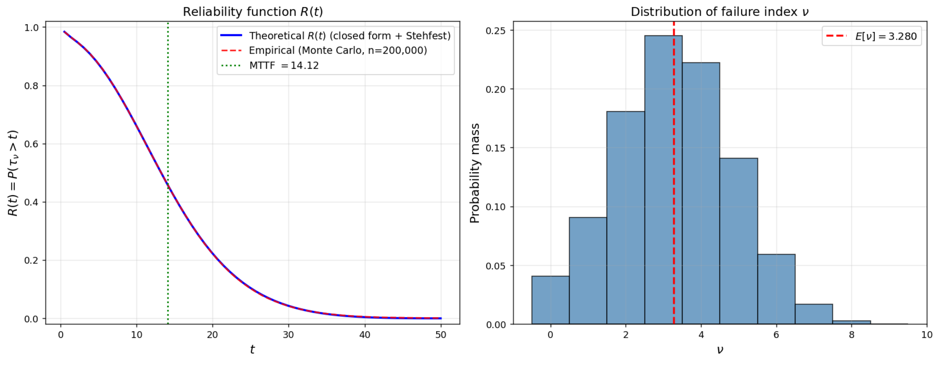
The Wald identities can be verified directly from the table: $\mathrm{MTTF}=1+4\times 3.280118=14.120472$ and $\mathbb{E}\left[S_{\nu }\right]=3.\overline{3}+2.5\times 3.280118=11.533628$, both matching their respective entries to numerical precision. The internal consistency relation $\mathrm{MTTF}=\mathbb{E}\left[{\tau }_{\nu -1}\right]+\mathbb{E}[{\tau }_{\nu }-{\tau }_{\nu -1}]=10.241532+3.878939=14.120471$ is also satisfied.

5.3. Monte Carlo Verification

To verify the closed-form expressions, we ran a Monte Carlo simulation of $N=2\times {10}^5$ independent trajectories. The simulation generates each trajectory by sampling $X_0$, $T_0$, then iteratively sampling $(T_n,X_n)$ until the cumulative damage exceeds the threshold; at each step, the relevant reliability quantities are recorded.

Table 3. Theoretical (closed-form) versus simulated values of the reliability indices over $N=2\times {10}^5$ Monte Carlo trajectories.

Quantity	Theoretical	Simulated	Error	95% MC SE
$\mathbb{E}\left[\nu \right]$	$3.280118$	$3.282075$	$0.001957$	$0.006927$
$\mathrm{MTTF}$	$14.120471$	$14.115045$	$0.005426$	$0.035917$
$\mathbb{E}\left[S_{\nu }\right]$	$11.533628$	$11.540545$	$0.006917$	$0.008767$
$\mathbb{E}[S_{\nu }-p_1]$	$2.533628$	$2.540545$	$0.006917$	$0.008767$
$\mathbb{E}\left[S_{\nu -1}\right]$	$7.333590$	$7.334450$	$0.000860$	$0.009706$
$\mathbb{E}\left[X_{\nu }\right]$	$4.200038$	$4.206095$	$0.006057$	$0.013429$
$\mathbb{E}\left[{\tau }_{\nu -1}\right]$	$10.241532$	$10.231517$	$0.010016$	$0.032954$
$\mathbb{E}[{\tau }_{\nu }-{\tau }_{\nu -1}]$	$3.878939$	$3.883529$	$0.004589$	$0.012455$

compares the empirical means against the theoretical values, together with the 95% Monte Carlo standard error.

For all eight indices, the absolute error between theoretical and simulated values is smaller than the 95% Monte Carlo standard error. This is the expected level of agreement for an unbiased estimator: the closed-form formulas are correct.

5.4. The Reliability Function

We compute the reliability function $R\left(t\right)=\mathbb{P}({\tau }_{\nu }>t)$ by numerical inversion of $\widehat{R}\left(\theta \right)=(1-{\widehat{F}}_{{\tau }_{\nu }}\left(\theta \right))/\theta$ via the Gaver–Stehfest algorithm (cf. [19,20]) with $N=14$ summation terms. Figure 1 (left) shows the resulting $R\left(t\right)$ together with the empirical reliability function from the Monte Carlo simulation.

The two curves are visually indistinguishable across the full time range $0<t<50$.

Table 4. Pointwise comparison of the theoretical reliability function $R\left(t\right)$ (Gaver–Stehfest inversion of the closed-form $\widehat{R}\left(\theta \right)$) versus the empirical $R\left(t\right)$ from the Monte Carlo simulation.

t	$\mathit{R}\left(\mathit{t}\right)$ Theoretical	$\mathit{R}\left(\mathit{t}\right)$ Simulated	Absolute Error
1	$0.972109$	$0.972100$	$0.000009$
2	$0.952221$	$0.952260$	$0.000039$
5	$0.872995$	$0.873645$	$0.000650$
10	$0.659651$	$0.659215$	$0.000436$
14	$0.462163$	$0.462430$	$0.000267$
20	$0.221970$	$0.220970$	$0.001000$
30	$0.042237$	$0.041445$	$0.000792$
50	$-0.000587$	$0.000380$	$0.000967$

reports a pointwise comparison.

The errors at all sampled times are at the level of Monte Carlo noise. The slight negative value at $t=50$ is a known artifact of the Gaver–Stehfest method when the inverted function approaches zero; it does not reflect an error in the closed-form $\widehat{R}\left(\theta \right)$ but the limited numerical precision of the inversion at large arguments. For applications requiring high accuracy in the far tail, alternative algorithms such as the Talbot or de Hoog method may be substituted; the closed-form $\widehat{R}\left(\theta \right)$ remains valid.

5.5. Phase-Resolved Failure Analysis

We illustrate the phase-resolved formulas of Section 4.4. By Theorem 8, the phase distribution at failure starting from phase $i\in \{1,2\}$ is

$$\mathbb{P}(J\left({\tau }_{\nu }\right)=j\mid J\left({\tau }_0\right)=i)=\mathbb{P}(X_0>p_1){\delta }_{ij}+\mathbb{P}(X_0\le p_1){\alpha }_j.$$

Numerically, with $\mathbb{P}(X_0>p_1)=0.04035$, $\mathbb{P}(X_0\le p_1)=0.95965$, and $\mathit{\alpha }=(1,0)$:

$$\begin{array}{ccc}\hfill {\left[\mathbb{P}(J\left({\tau }_{\nu }\right)=j\mid J\left({\tau }_0\right)=i)\right]}_{ij}& =& \left(\begin{array}{cc}0.04035·1+0.95965·1& 0.04035·0+0.95965·0\\ 0.04035·0+0.95965·1& 0.04035·1+0.95965·0\end{array}\right)\hfill \\ & =& \left(\begin{array}{cc}1& 0\\ 0.95965& 0.04035\end{array}\right).\hfill \end{array}$$

The first row reflects the deterministic case $\mathit{\alpha }=(1,0)$: every shock initiates in phase 1. The second row reveals the phase-resolution structure: starting in phase 2, the system fails in phase 2 with probability $0.04035$ (the probability of immediate failure, in which the initial phase is preserved), and in phase 1 with probability $0.95965$ (the probability of delayed failure, in which the post-delay shock-renewal mechanism resamples the phase from $\mathit{\alpha }$).

For the phase-resolved failure-time distribution (51), the LST decomposes additively as

$$\mathbb{E}[e^{-\theta {\tau }_{\nu }}{\mathbf{1}}_{\{J\left({\tau }_{\nu }\right)=j\}}\mid J\left({\tau }_0\right)=i]=\underset{\mathrm{i}\mathrm{m}\mathrm{m}\mathrm{e}\mathrm{d}\mathrm{i}\mathrm{a}\mathrm{t}\mathrm{e}\text{-}\mathrm{f}\mathrm{a}\mathrm{i}\mathrm{l}\mathrm{u}\mathrm{r}\mathrm{e}\mathrm{piece}}{\underbrace{h_0\left(\theta \right)\mathbb{P}(X_0>p_1){\delta }_{ij}}}+\underset{\mathrm{d}\mathrm{e}\mathrm{l}\mathrm{a}\mathrm{y}\mathrm{e}\mathrm{d}\text{-}\mathrm{f}\mathrm{a}\mathrm{i}\mathrm{l}\mathrm{u}\mathrm{r}\mathrm{e}\mathrm{piece}}{\underbrace{h_0\left(\theta \right)v_i\left(\theta \right){\alpha }_{j}G\left(\theta \right)}}.$$

At $\theta =0$ the right-hand side reduces to the entrywise phase distribution computed above (since $h_0\left(0\right)=1$, $v_i\left(0\right)=1$, $G\left(0\right)=\mathbb{P}(X_0\le p_1)$). For $\theta >0$, the formula provides the joint Laplace-domain characterization of (failure time, end phase). For example, at $\theta =0.1$, starting from phase $i=1$, conditional on ending in phase $j=1$:

$$\mathbb{E}[e^{-0.1{\tau }_{\nu }}{\mathbf{1}}_{\{J\left({\tau }_{\nu }\right)=1\}}\mid J\left({\tau }_0\right)=1]=h_0\left(0.1\right)·0.04035+h_0\left(0.1\right)v_1\left(0.1\right){\alpha }_{1}G\left(0.1\right)\approx 0.323,$$

which matches the unconditional ${\widehat{F}}_{{\tau }_{\nu }}\left(0.1\right)$ in this $\mathit{\alpha }=(1,0)$ instance, since all simulation mass is concentrated on the $i=j=1$ entry.

The phase-resolved decomposition is most informative when $\mathit{\alpha }$ has full support: in such cases, the immediate-failure piece is concentrated on the diagonal $(i=j)$ while the delayed-failure piece distributes mass according to the rank-one $v_i\left(\theta \right){\alpha }_j$ pattern, providing a complete operational picture of how failures are distributed across operational regimes.

5.6. Discussion

The numerical example demonstrates three points relevant to the contributions of the paper.

First, computational tractability. All twelve reliability indices in Table 1 were computed in elementary arithmetic without any iterative matrix solver. The most expensive operation is the Gaver–Stehfest inversion at each plotted time point, which requires $O\left(N{p}_1\right)$ operations per evaluation; closed-form values such as $\mathrm{MTTF}$ and $\mathbb{E}\left[\nu \right]$ are essentially instantaneous to evaluate. The $\mathfrak{D}$-operator algorithm of Appendix B extends to any rational PGFs $a_0, a$ and rational LSTs $h_0, h$; these cover all phase-type, shifted-geometric, negative-binomial, and discrete phase-type combinations that appear in the cumulative shock literature.

Second, closed-form versus simulation. The agreement between closed-form values and Monte Carlo is at the level of Monte Carlo noise across all reliability indices and across the full reliability function $R\left(t\right)$. While Monte Carlo would always be available as a fallback, the closed-form formulas provide $O\left({10}^7\right)$-fold speed gains over $N=2\times {10}^5$ simulation, with no statistical error and full availability of derivatives (sensitivities) by direct differentiation.

Third, phase-resolved insight. The closed form for $\mathbb{P}(J\left({\tau }_{\nu }\right)=j\mid J\left({\tau }_0\right)=i)$ in this two-phase example reveals the immediate/delayed failure cleavage transparently. In more general PH structures with a non-degenerate initial vector $\mathit{\alpha }$, the same decomposition gives a complete operational breakdown of failure events by ending phase, a quantity that is—to our knowledge—not directly available in the standard matrix-analytic reliability literature [9,10,12], where the analysis of repairable systems via QBD methods focuses on steady-state availability and the rate of occurrence of failures rather than on first-passage joint distributions.

6. Discussion and Extensions

This section situates the contributions of the paper in the broader reliability and applied-probability literature, addresses two natural extensions of the framework, and outlines directions for follow-up work.

6.1. Position in the Literature

The reliability community has developed two largely separate analytic traditions for systems subject to random shocks.

6.1.1. Fluctuation-Theoretic Tradition

The first tradition treats the failure event as a first-passage event of a marked point process. Foundational work of [1,4] established the cumulative shock model as a tractable analytical framework. The first-passage functional approach was substantially developed by [5,6], with explicit transforms for the joint distribution of failure time, overshoot, and pre-failure quantities. Refs. [3,7] extended the framework to mixed soft- and hard-shock systems with linear degradation, and Ref. [8] treated dependent competing failure processes in this language. Ref. [17] and the broader shock-model literature surveyed in [2] provide complementary results within this tradition. Recent extensions of cumulative shock theory include protection mechanisms with practical applications to wind-turbine reliability [21], distributional analyses of discrete censored $\delta$-shock variants [22], and dependent shock magnitudes [23]. The strength of the fluctuation-theoretic approach is the closed-form availability of the joint distribution of failure-time observables; its limitation, until now, has been an inability to incorporate the matrix structure that phase-type or Markov-modulated inter-shock dynamics naturally produce.

6.1.2. Matrix-Analytic Tradition

The second tradition originates in the work of [9] and is comprehensively presented in [10]. Phase-type, Markov-modulated, and quasi-birth-death (QBD) representations have been applied to a wide range of reliability problems: k-out-of-n:G systems, redundant systems with switching, repairable systems with vacations, and multi-component networks. The recent series of [11,12] exemplifies the contemporary state of the art, treating k-out-of-n:G repairable systems with K-mixed redundancy and repairman vacations under PH lifetime, repair, and vacation distributions. Related contributions in the same period [13,14,15] develop matrix-distributed and MAP-driven shock models that share our discrete phase-type machinery while pursuing distinct analytical objectives. The strength of the matrix-analytic approach is its ability to handle complex multi-component repair structures with phase information; its limitation has been a focus on stationary indicators (availability, ROCOF) rather than first-passage joint distributions.

6.1.3. The Phase-Tagged Framework as a Bridge

The phase-tagged first excess theory of [16] occupies the intersection of these traditions: it inherits the closed-form fluctuation analysis of the Dshalalow lineage while introducing the matrix-valued phase-tagging of the Neuts lineage. The present paper applies this bridge to cumulative shock reliability, producing the first closed-form results for the joint distribution of (failure time, overshoot, pre-failure quantities, end phase) under PH inter-shock times.

Table 5. Position of the present framework relative to the two existing analytical traditions for shock-driven reliability systems.

	Closed-Form	PH Inter-Shocks	Phase Tagging
	First Passage		at Failure
Cumulative shock fluctuation analysis	✓	—	—
([3,5])
Matrix-analytic reliability (QBD-based)	—	✓	—
([9,12])
Phase-tagged first excess ([16])	✓	✓	✓
This paper (matrix lift with pre-failure)	✓	✓	✓

summarizes the position.

6.2. Extension to Position-Dependent Marking

Assumption 1 requires the damage sequence $\left\{X_n\right\}$ to be independent of the inter-shock time sequence $\left\{T_n\right\}$. This is the analogue of the independent-marks assumption in marked-point-process language. Refs. [3,5] treat the more general setting of position-dependent marking, in which $X_n$ may depend on $T_n$ via a joint transform $\gamma (z,\eta )=\mathbb{E}\left[z^{X_n}{e}^{-\eta T_n}\right]$ that does not factor as $a\left(z\right)h\left(\eta \right)$.

In the matrix-tagged framework, position-dependent marking corresponds to replacing the scalar PGF a and the matrix LST $H\left(\theta \right)$ by a single matrix-valued joint transform

$$\mathbf{\Gamma }{(z,\eta )}_{ij}=\mathbb{E}\left[z^{X_n}{e}^{-\eta T_n}{\mathbf{1}}_{\{J\left({\tau }_n\right)=j\}}|J\left({\tau }_{n-1}\right)=i\right],$$

which captures the joint distribution of damage, inter-shock time, and the phase transition in a single object. The derivation of Theorem 1 carries through up to the matrix geometric series (26), but the Sherman–Morrison reduction (27) and the mixed-LST identity (5) no longer apply in their present form: $\mathbf{\Gamma }(z,\eta )$ is not generally rank-one in z, and the rank-one structure of $H\left(\theta \right)=\mathbf{v}\left(\theta \right)\mathit{\alpha }$ is what produces the closed-form three-dimensional span of Theorem 2.

Therefore, the position-dependent case admits a structural representation

$${\mathbf{\Phi }}_{\nu }^{\mathrm{pd}}(\xi ,u,v,\vartheta ,\theta )=\left(\mathrm{i}\mathrm{m}\mathrm{m}\mathrm{e}\mathrm{d}\mathrm{i}\mathrm{a}\mathrm{t}\mathrm{e}\text{-}\mathrm{e}\mathrm{x}\mathrm{c}\mathrm{e}\mathrm{s}\mathrm{s}\right)+{\mathfrak{D}}_x^{p_1}\left\{\xi a_0\left(uvx\right)(\cdots ){\left(I-\xi \mathbf{\Gamma }(uvx,\vartheta +\theta )\right)}^{-1}\mathbf{\Gamma }(v,\theta )\right\},$$

in which the inverse ${(I-\xi \mathbf{\Gamma }(uvx,\omega ))}^{-1}$ is a general $m\times m$ matrix inverse rather than a rank-one Sherman–Morrison reduction. Such an inverse is computable but does not in general admit a low-dimensional span representation, and the elegant Wald-type identities of Theorems 6 and 7 do not survive without modification.

A natural special case in which the position-dependent framework retains tractability is when the dependence between $X_n$ and $T_n$ is mediated solely by the phase $J\left({\tau }_n\right)$: that is, conditional on $J\left({\tau }_n\right)=k$, the damage $X_n$ has phase-dependent PGF $a_k\left(z\right)$ but is otherwise independent of $T_n$. In this case, $\mathbf{\Gamma }(z,\eta )$ retains a rank-one factorization when restricted to each terminal phase, and a phase-stratified version of the closed form can be obtained. This direction extends the framework toward the BMAP-style structure used in subsequent papers by the authors of [16] and is left for follow-up work.

6.3. Extension to Repairable and Multi-Component Systems

The cumulative shock model treated in this paper describes a non-repairable single-component system: the cumulative damage process is monotone non-decreasing, and the failure event is absorbing. The most natural extension is to repairable systems, in which the cumulative damage may be reset (or partially reset) at intervention epochs.

In the matrix-analytic reliability literature, repairable systems are typically analyzed via QBD methods that yield stationary availability and ROCOF; the framework of [12] for k-out-of-n:G systems with repairman vacations is a representative example. Bringing the phase-tagged framework to bear on repairable systems requires extending the threshold-crossing event structure: rather than the first passage of a monotone process, one studies the first passage of an embedded regenerative process. This corresponds in queueing terms to passing from cumulative-shock first-excess to busy-period or sojourn-time analysis. The phase-tagged formalism extends naturally; the matrix-valued first-passage functionals admit similar closed-form representations under PH inter-event distributions, but a complete development is beyond the scope of the present paper.

A second natural extension is to multi-component systems, including k-out-of-n:G structures. The single-threshold first-excess event $\{S_{\nu }>p_1\}$ generalizes to a multi-dimensional crossing event of the type studied by [24] for vector renewal processes. The matrix-tagged generalization of these multi-dimensional first-excess functionals would directly produce closed-form reliability indices for k-out-of-n:G systems with phase-type component lifetimes and repair-time distributions, providing a fluctuation-theoretic counterpart to the QBD analyses of [11,12]. A third direction concerns dependent failure processes in which degradation and shock arrivals interact, as studied recently by [25] for systems with self-healing and [26] for continuous fatigue degradation coupled to shock arrivals via a Markov renewal process. Extending the phase-tagged functional to track both the cumulative shock process and a coupled degradation process simultaneously is a natural avenue for future work in this direction.

6.4. Methodological Observations

We close with two methodological observations that may be useful in subsequent applications of the framework.

6.4.1. Span Dimension as a Structural Invariant

Theorem 2 shows that ${\mathbf{\Phi }}_{\nu }$ lies in a three-dimensional matrix subspace, generalizing the two-dimensional span of [16]. The dimension counts the distinct “time scales” tracked by the functional: $\mathbf{\Psi }(\xi ,\theta ,u)$ tracks one (the failure time), while ${\mathbf{\Phi }}_{\nu }(\xi ,u,v,\vartheta ,\theta )$ tracks two (failure time ${\tau }_{\nu }$ and pre-failure time ${\tau }_{\nu -1}$). This pattern suggests that further enrichment of the functional, for example, joint distribution of ${\tau }_{\nu }$, ${\tau }_{\nu -1}$, and a third intermediate epoch ${\tau }_{\nu -2}$, would produce a four-dimensional span $\mathrm{span}\{I,H\left(\theta \right),H\left(\omega \right),H(\omega +{\vartheta }^{\prime })\}$ for some additional time variable ${\vartheta }^{\prime }$. The span dimension is therefore a structural invariant indexing how many time variables the analyst chooses to track. Computational cost grows with this dimension only through the addition of independent scalar coefficients; the underlying algebra remains tractable.

6.4.2. Reliability Indices and Wald-Type Identities

The two structural identities, Theorem 6 for $\mathrm{MTTF}={\mu }_{T_0}+{\mu }_T\mathbb{E}\left[\nu \right]$ and Theorem 7 for $\mathbb{E}\left[S_{\nu }\right]=\mathbb{E}\left[X_0\right]+{\mu }_A\mathbb{E}\left[\nu \right]$, are not artifacts of our particular model: they reflect the underlying renewal-and-stopping structure of any cumulative-shock system with independent damage variables and inter-shock times. The extraction of these identities from Theorem 1 via the $\mathfrak{D}$-operator algebra illustrates a methodological point: closed-form first-passage transforms, when present, automatically yield Wald-type structural identities as corollaries of differentiation at the origin. Future applications of the phase-tagged framework to other reliability models should expect similar identities to emerge.

7. Conclusions

This paper has developed a closed-form analysis of the joint distribution for cumulative shock reliability systems with phase-type inter-shock times, resolving a methodological gap between the scalar fluctuation-theoretic and matrix-analytic traditions for shock-driven reliability. We summarize the contributions, the structural observations, and the directions for future work.

7.1. Principal Contributions

The paper makes four main contributions.

(1)

A matrix-valued reliability functional. We introduced ${\mathbf{\Phi }}_{\nu }(\xi ,u,v,\vartheta ,\theta )$, the joint transform of the failure index, pre-failure damage and time, failure-time damage and time, and the operational phase at the moment of failure, conditional on the initial phase. Theorem 1 provides the closed-form expression via Sherman–Morrison reduction of the matrix Laplace–Stieltjes transform together with the Dshalalow $\mathfrak{D}$-operator.

(2)

A bridge between two analytical traditions. The framework simultaneously generalizes the scalar fluctuation functional of [3,5] (Theorem 4) and extends the phase-tagged first excess functional of [16] to incorporate pre-failure quantities (Theorem 3). Both consistency relations are established by direct algebraic reduction from Theorem 1.

(3)

Twelve closed-form reliability indices. From ${\mathbf{\Phi }}_{\nu }$ we extracted twelve indices in closed form: the failure-time LST, reliability function, mean time to failure, mean cumulative damage and overshoot, mean pre-failure damage and time, mean failure-causing inter-shock interval, mean failure-causing shock magnitude, joint LSTs and PGFs of pre-failure and failure pairs, and, new to the cumulative shock literature, the phase distribution at failure and the phase-resolved failure-time distribution.

(4)

Wald-type structural identities. Two identities emerged as corollaries: $\mathrm{MTTF}={\mu }_{T_0}+{\mu }_T\mathbb{E}\left[\nu \right]$ for total mean failure time, and $\mathbb{E}\left[S_{\nu }\right]=\mathbb{E}\left[X_0\right]+{\mu }_A\mathbb{E}\left[\nu \right]$ for total mean damage. Both express their target in terms of the fundamental scalar $\mathbb{E}\left[\nu \right]$, which admits an explicit $\mathfrak{D}$-operator representation.

7.2. Structural Observation

A notable feature of the closed form is the span structure of Theorem 2: the matrix functional ${\mathbf{\Phi }}_{\nu }$ lies in the three-dimensional subspace $\mathrm{span}\{I,H(\theta ),H(\omega \left)\right\}$, generalizing the two-dimensional span of [16]. The third basis element $H\left(\omega \right)$ encodes the joint pre-failure-time/failure-time tracking; in its absence ($\vartheta =0$) the span collapses to two dimensions. We conjectured (Section 6.4) that further enrichment of the functional with intermediate epoch tracking would produce higher-dimensional spans of analogous form, with the dimension serving as a structural invariant counting the number of time scales monitored by the analyst.

7.3. Numerical Verification

A worked example with two-phase Erlang inter-shock times, exponential delay, and shifted-geometric damages (Section 5) verified all closed-form reliability indices against $2\times {10}^5$ Monte Carlo trajectories, with all errors below the 95% Monte Carlo standard error, and exhibited the reliability function $R\left(t\right)$ obtained by Gaver–Stehfest inversion of the closed-form $\widehat{R}\left(\theta \right)$.

7.4. Future Work

Several extensions are natural and were sketched in Section 6.

• Position-dependent marking and continuous damage. Position-dependent marking (in which damages depend on inter-shock times) breaks the rank-one structure of $H\left(\theta \right)$, but tractable cases mediated by the phase variable connect to the BMAP-style extensions developed in subsequent work. The continuous-damage case, in which the PGF $a\left(u\right)=\mathbb{E}\left[u^X\right]$ is replaced by the Laplace transform $\tilde{a}\left(\eta \right)=\mathbb{E}\left[e^{-\eta X}\right]$, is a parallel direction.
• Repairable and multi-component systems. The framework extends naturally to k-out-of-n:G structures via vector first-excess processes [24], providing a fluctuation-theoretic counterpart to the QBD analyses of [11,12].
• Dependent shock-degradation processes. The framework also admits extension to settings where degradation and shock arrivals interact, as studied recently by [25,26].

7.5. Methodological Scope

Beyond reliability, the methodological pattern illustrated here (lifting a scalar fluctuation functional to matrix form, exploiting the rank-one structure of $H\left(\theta \right)$ to maintain Sherman–Morrison tractability, then extract observables via $\mathfrak{D}$-operator algebra) applies to any domain where first-passage joint distributions of cumulative processes are of interest. Inventory theory, insurance risk, dam and storage models, and Markov-modulated finance all fit this template. The phase-tagged framework provides a uniform analytical apparatus across these settings, with the present paper supplying a worked-out reliability instance and a template for further applications.

References

1. Esary, J.D.; Marshall, A.W.; Proschan, F. Shock models and wear processes. Ann. Probab. 1973, 1, 627–649. [Google Scholar] [CrossRef] [Scilit]
2. Nakagawa, T. Shock and Damage Models in Reliability Theory; Springer: London, UK, 2007. [Google Scholar]
3. Dshalalow, J.H.; White, R.T. Random walk analysis in a reliability system under constant degradation and random shocks. Axioms 2021, 10, 199. [Google Scholar] [CrossRef] [Scilit]
4. Gut, A. Cumulative shock models. Adv. Appl. Probab. 1990, 22, 504–507. [Google Scholar] [CrossRef] [Scilit]
5. Abolnikov, L.; Dshalalow, J.H. A first passage problem and its applications to the analysis of a class of stochastic models. J. Appl. Math. Stoch. Anal. 1992, 5, 83–98. [Google Scholar] [CrossRef] [Scilit]
6. Dshalalow, J.H. Excess level processes in queueing. In Advances in Queueing: Theory, Methods, and Open Problems; Dshalalow, J.H., Ed.; CRC Press: Boca Raton, FL, USA, 1995; pp. 243–262. [Google Scholar]
7. Dshalalow, J.H.; White, R.T. Fluctuation analysis of a soft-extreme shock reliability model. Mathematics 2022, 10, 3312. [Google Scholar] [CrossRef] [Scilit]
8. Dshalalow, J.H.; Aljahani, H.; White, R.T. Dependent competing failure processes in reliability systems. Entropy 2024, 26, 444. [Google Scholar] [CrossRef] [Scilit] [PubMed]
9. Neuts, M.F. Structured Stochastic Matrices of M/G/1 Type and Their Applications; Marcel Dekker: New York, NY, USA, 1989. [Google Scholar]
10. Latouche, G.; Ramaswami, V. Introduction to Matrix Analytic Methods in Stochastic Modeling; SIAM and ASA: Philadelphia, PA, USA, 1999. [Google Scholar]
11. Wen, Y.; Liu, B.; Zhang, Z.; Shi, H.; Kang, S. Modeling and analysis for a repairable system with multi-state components under K-mixed redundancy strategy. Commun. Stat. Theory Methods 2024, 53, 748–764. [Google Scholar] [CrossRef] [Scilit]
12. Wen, Y.; Liu, B.; Qiu, Q.; Shang, L.; Gao, Y. Matrix-analytic reliability modeling of k-out-of-n:G repairable systems with K-mixed redundancy and repairman’s multiple vacations. Reliab. Eng. Syst. Saf. 2026, 275, 112781. [Google Scholar] [CrossRef] [Scilit]
13. Goyal, D.; Hazra, N.K.; Finkelstein, M. Shock models based on renewal processes with matrix Mittag-Leffler distributed inter-arrival times. J. Comput. Appl. Math. 2024, 435, 115090. [Google Scholar] [CrossRef] [Scilit]
14. Goyal, D.; Ali, R.; Hazra, N.K. Reliability analysis of δ-shock models based on the Markovian arrival process. Appl. Stoch. Models Bus. Ind. 2024, 40, 1291–1312. [Google Scholar] [CrossRef] [Scilit]
15. Hu, Z.; Hu, L. Reliability assessment of a multi-state mixed δ-shock model based on discrete phase-type distribution. Ann. Oper. Res. 2025, 353, 885–916. [Google Scholar] [CrossRef] [Scilit]
16. Tadj, L. Phase-tagged first excess level theory: A matrix-analytic bridge to Dshalalow’s fluctuation functional. 2025; submitted.
17. Eryilmaz, S. Discrete time shock models in a Markovian environment. IEEE Trans. Reliab. 2016, 65, 141–146. [Google Scholar] [CrossRef] [Scilit]
18. Sherman, J.; Morrison, W.J. Adjustment of an inverse matrix corresponding to a change in one element of a given matrix. Ann. Math. Stat. 1950, 21, 124–127. [Google Scholar] [CrossRef] [Scilit]
19. Stehfest, H. Algorithm 368: Numerical inversion of Laplace transforms. Commun. ACM 1970, 13, 47–49. [Google Scholar] [CrossRef] [Scilit]
20. Abate, J.; Whitt, W. Numerical inversion of Laplace transforms of probability distributions. ORSA J. Comput. 1995, 7, 36–43. [Google Scholar] [CrossRef] [Scilit]
21. Eryilmaz, S. A class of shock models for a system that is equipped with a protection block, with an application to wind turbine reliability. Appl. Stoch. Models Bus. Ind. 2025, 41, e70051. [Google Scholar] [CrossRef] [Scilit]
22. Chadjiconstantinidis, S.; Eryilmaz, S. Distributions of random variables involved in discrete censored δ-shock models. Adv. Appl. Probab. 2023, 55, 1144–1170. [Google Scholar] [CrossRef] [Scilit]
23. Eryilmaz, S. The evaluation of system reliability under dependent shock magnitudes. Methodol. Comput. Appl. Probab. 2026, 28, 22. [Google Scholar] [CrossRef] [Scilit]
24. Dshalalow, J.H. First excess levels of vector processes. J. Appl. Math. Stoch. Anal. 1994, 7, 457–464. [Google Scholar] [CrossRef] [Scilit]
25. Kang, F.; Cui, L.; Ye, Z.; Zhou, Y. Reliability analysis for systems with self-healing mechanism in degradation-shock dependence processes with changing degradation rate. Reliab. Eng. Syst. Saf. 2024, 241, 109627. [Google Scholar] [CrossRef] [Scilit]
26. Jiang, S.; Jia, X. Reliability assessment under continuous fatigue degradation and shock based on Markov renewal process. Reliab. Eng. Syst. Saf. 2024, 248, 110151. [Google Scholar] [CrossRef] [Scilit]
Figure 1. (Left): theoretical reliability function R ( t ) obtained by closed-form computation of R ^ ( θ ) and Gaver–Stehfest inversion (solid blue), versus the empirical reliability function from N = 2 × 10 5 Monte Carlo trajectories (dashed red). The vertical dotted line marks MTTF = 14.12 . (Right): empirical distribution of the failure index ν from the Monte Carlo simulation, with the theoretical mean E [ ν ] = 3.280 marked.
Mathematics 14 01920 g001