The Touchard Process for Count Data with Dependent Increments

Abstract

This paper introduces the Touchard process, a flexible two-parameter stochastic framework for modeling count data that depart from the classical Poisson assumptions. In contrast to standard Poisson processes, the proposed model allows for both nonstationary and dependent increments, enabling the representation of overdispersion, underdispersion, and temporal dependence within a unified structure. The main contribution lies in extending weighted Poisson models to a stochastic-process setting through recursively defined transition probabilities associated with Touchard marginal distributions. We derive key theoretical properties, including admissibility conditions and a recursive formulation for the transition probabilities, and propose an efficient simulation algorithm. Maximum likelihood estimation is developed for parameter inference, and a likelihood ratio framework is used for model comparison. An empirical application to motor vehicle crash data illustrates the ability of the model to capture dynamic patterns that are not adequately described by classical Poisson-based approaches.

1. Introduction

The Poisson process is a classical counting model that has been applied across various fields [1,2,3,4,5]. It relies on the assumptions of stationarity and independent increments, implying that events occur at a constant rate and are mutually independent. However, many real-world phenomena violate these assumptions. As underlying processes evolve, increments may become nonstationary and serially dependent, leading to patterns such as overdispersion, underdispersion, or zero inflation, which the standard Poisson process cannot accommodate [6].

To capture such deviations, more flexible models are needed that preserve the counting nature of the process while relaxing its classical assumptions. Numerous generalizations of the Poisson distribution have been proposed (e.g., [7,8,9,10,11,12,13,14,15,16,17,18,19,20,21,22]), many of which serve as the foundation for regression and time-series models (e.g., [19,23,24,25,26,27,28,29]). While these approaches allow for flexible marginal distributions and can incorporate temporal dependence through model structures, they typically do not provide an explicit process-based construction in which dispersion and dependence arise endogenously from the increment dynamics. In particular, the joint modeling of nonstationarity, dependence, and dispersion within a unified stochastic framework remains relatively limited.

A notable exception is the class of weighted Poisson distributions [22,26,30], which incorporates weight functions to modify Poisson probabilities, thereby capturing scenarios with excess variability or clustering. This approach links the properties of the data to correlation structures and dependencies in the underlying process, offering a richer analytical framework. Balakrishnan and Kozubowski [30] showed that overdispersion and underdispersion in counts are related to correlations in process increments. Nevertheless, the assumption of stationary increments remains restrictive in many practical applications.

Beyond count regression and time-series formulations, there is increasing interest in stochastic process models that can represent heterogeneous evolution, dependence structures, and nonstationary dynamics in complex systems. This includes nonhomogeneous Poisson processes, doubly stochastic Poisson (Cox) processes, and INGARCH-type autoregressive count models, which incorporate time-varying intensities and serial dependence through different mechanisms [31,32,33,34,35]. Similar challenges also arise in reliability analysis and degradation modeling, where stochastic mechanisms may exhibit initiation-growth correlations, heterogeneous degradation trajectories, and time-varying variability [36,37].

In this paper, we introduce the Touchard process, a two-parameter extension of the Poisson process based on the Touchard probability distribution [18,26,38]. It belongs to the class of weighted Poisson processes but relaxes the stationary and independent increments assumption by recursively defining transition probabilities. As a generalization of the Poisson process, the additional parameter ${\delta }_t$ controls the dispersion structure, while ${\lambda }_t$ governs the process mean. Consequently, unlike the classical Poisson process, the Touchard process can accommodate overdispersion, underdispersion, and count data with excess zeros. Combined with its nonstationary behavior and dependence among increments, this formulation expands the range of count dynamics that can be represented within a unified stochastic-process framework.

By combining mathematical tractability with enhanced adaptability, the Touchard process expands the toolkit for modeling count data. Its formulation enables researchers to align models more closely with empirical characteristics, thereby improving inference and interpretation. In this context, the focus of this work is to examine how deviations from the classical assumptions of stationary and independent increments affect the behavior of count processes. The Poisson process is therefore adopted as a natural baseline, as it provides the canonical reference under these assumptions, allowing us to isolate the impact of introducing dependence, nonstationarity, and dispersion within the proposed framework.

From a modeling perspective, the Touchard process also differs conceptually from other counting-process constructions with dependent increments, such as Hawkes, Cox, or INAR-type models. In those approaches, dependence is typically introduced through self-exciting intensities, latent stochastic environments, or autoregressive thinning mechanisms. In contrast, the Touchard process is constructed by specifying Touchard marginal distributions together with recursively defined transition probabilities, yielding a coherent stochastic-process framework with nonstationary and dependent increments. Although the process is characterized through its marginal distributions and transition structure, the resulting formulation provides additional insight beyond cross-sectional fitting by explicitly modeling the temporal evolution of the counts, allowing transition probabilities, aggregation effects, and dependence structures to be analyzed within a unified probabilistic framework.

Section 2 describes the Touchard process, detailing the process rate and deriving the probabilities of nonstationary, dependent increments using a recursive formula. Section 3 presents an algorithm for simulating the Touchard process and illustrates how the transition probabilities evolve. To exemplify its practical applicability, we analyze daily accident count data from the New York State Department of Motor Vehicles (NY DMV), recorded in 5-min intervals from 6:00 p.m. to 7:00 p.m. across Queens and Kings Counties during 2018–2022 (Section 5).

2. The Touchard Process

In this section, we introduce the Touchard process and establish its main probabilistic properties. We begin by defining the Touchard marginal distribution and showing its connection with weighted Poisson models. We then derive the corresponding process structure by recursively defining transition probabilities that induce nonstationary and dependent increments. Finally, we discuss the admissibility conditions required for the resulting recursive construction to define a valid stochastic counting process.

Definition 1

(Touchard Marginal Distribution). Let $t\ge 0$. A discrete random variable $X\left(t\right)$ is said to follow a Touchard distribution if its probability mass function is given by

$$\begin{array}{c}\hfill p_k\left(t\right)=P[X\left(t\right)=k]={\displaystyle \frac{{\lambda }_t^k{(k+1)}^{{\delta }_t}}{k!\tau ({\lambda }_t,{\delta }_t)}},k\in \mathbb{N},\end{array}$$

(1)

where ${\lambda }_t>0$ and ${\delta }_t\in \mathbb{R}$ are time-dependent parameters, and 

$$\begin{array}{c}\hfill \tau ({\lambda }_t,{\delta }_t)=\sum _{j\in \mathbb{N}}{\displaystyle \frac{{\lambda }_t^j{(j+1)}^{{\delta }_t}}{j!}}\end{array}$$

(2)

is the corresponding normalizing function.

We remark that when ${\delta }_t=0$, we have $\tau ({\lambda }_t,0)={\sum }_{j\in \mathbb{N}}{\lambda }_t^j/j!={\mathrm{e}}^{{\lambda }_t}$, and (1) reduces to the classical Poisson probability mass function $p_k\left(t\right)={\mathrm{e}}^{-{\lambda }_t}{\lambda }_t^k/k!$. Consequently, under ${\delta }_t=0$, the proposed Touchard process will recover the classical Poisson process model.

The normalizing function (2) is finite for all finite ${\lambda }_t>0$ and ${\delta }_t\in \mathbb{R}$. Indeed, applying the ratio test to the series terms $a_j={\lambda }_t^j{(j+1)}^{{\delta }_t}/j!$, gives

$$\begin{array}{c}\hfill {\displaystyle \frac{a_{j+1}}{a_j}}={\displaystyle \frac{{\lambda }_t}{j+1}}{\left({\displaystyle \frac{j+2}{j+1}}\right)}^{{\delta }_t}⟶0,j\to \infty ,\end{array}$$

so the series converges absolutely. In particular, $X\left(t\right)$ represents a random count of events as a function of exposure to a time window of length t.

Definition 2

(Touchard Process). The Touchard process is a discrete-time counting process whose finite-dimensional structure is characterized by Touchard marginal distributions and recursively specified transition probabilities (defined later in Proposition 3), allowing for dependent and nonstationary increments.

Thus, when the exposure interval has zero length, it is natural to impose the initial conditions

$$\begin{array}{c}\hfill P[X\left(0\right)=0]=1,{\lambda }_0=0\mathrm{and}\tau ({\lambda }_0,{\delta }_0)=1.\end{array}$$

(3)

From the marginal distribution defined in (1) and (2), the corresponding mean and variance functions are given by

$$\begin{array}{c}\hfill {\mu }_t={\displaystyle \frac{\tau ({\lambda }_t,{\delta }_t+1)}{\tau ({\lambda }_t,{\delta }_t)}}-1,\end{array}$$

(4)

and

$$\begin{array}{c}\hfill {\sigma }_t^2={\displaystyle \frac{\tau ({\lambda }_t,{\delta }_t+2)}{\tau ({\lambda }_t,{\delta }_t)}}-{({\mu }_t+1)}^2,\end{array}$$

(5)

with overdispersion (${\sigma }_t^2/{\mu }_t>1$) occurring when ${\delta }_t<0$, and underdispersion (${\sigma }_t^2/{\mu }_t<1$) occurring when ${\delta }_t>0$ [18,26].

If ${\lambda }_t$ and ${\delta }_t$ are differentiable functions of t, except possibly at a finite or countable set of time points, the time derivative of (1) results in a simplified rate equation form

$$\begin{array}{cc}\hfill {\dot{p}}_k\left(t\right)& ={\displaystyle \frac{\mathrm{d}}{\mathrm{d}t}}{p}_k\left(t\right)=-{\mathrm{\Lambda }}_k\left(t\right)p_k\left(t\right),\hfill \end{array}$$

(6)

where $k\ge 0$ and

$$\begin{array}{cc}\hfill {\mathrm{\Lambda }}_k\left(t\right)& =\left\{{\displaystyle \frac{\dot{\tau }({\lambda }_t,{\delta }_t)}{\tau ({\lambda }_t,{\delta }_t)}}-k{\displaystyle \frac{{\dot{\lambda }}_t}{{\lambda }_t}}-{\dot{\delta }}_{t}ln(k+1)\right\}\hfill \end{array}$$

denotes the rate function associated with state k at time t. As a counting process with non-negative increments, the mean ${\mu }_t$ has to be a positive and increasing function of time. Thus, using (6), we find

$$\begin{array}{cc}\hfill {\dot{\mu }}_t& ={\displaystyle \frac{\mathrm{d}}{\mathrm{d}t}}{\mu }_t={\displaystyle \frac{\mathrm{d}}{\mathrm{d}t}}\sum _{k\ge 0}k{p}_k\left(t\right)=\sum _{k\ge 0}k{\dot{p}}_k\left(t\right)\hfill \\ \hfill & ={\displaystyle \frac{{\dot{\lambda }}_t}{{\lambda }_t}}{\sigma }_t^2+{\dot{\delta }}_t{\gamma }_t,\hfill \end{array}$$

(7)

where

$$\begin{array}{c}\hfill {\gamma }_t=Cov\left[X\left(t\right),ln\left(X\right(t)+1)\right]>0,\end{array}$$

(8)

provided that ${\sigma }_t^2>0$, since $ln\left(X\right(t)+1)$ is a strictly increasing function of $X\left(t\right)$. As ${\lambda }_t$ drives ${\mu }_t$, it must satisfy ${\dot{\lambda }}_t>0$ [18]. Thus, from (7), to ensure ${\dot{\mu }}_t>0$, we assume

$$\begin{array}{c}\hfill {\dot{\delta }}_t>-{\displaystyle \frac{{\dot{\lambda }}_t{\sigma }_t^2}{{\lambda }_t{\gamma }_t}}.\end{array}$$

(9)

The condition in (9) is consistent with the admissibility requirements discussed below for the recursively defined transition probabilities. In particular, the simulation studies and empirical applications were conducted under parameter configurations satisfying these admissibility conditions, ensuring that the resulting transition probabilities define a proper stochastic counting process.

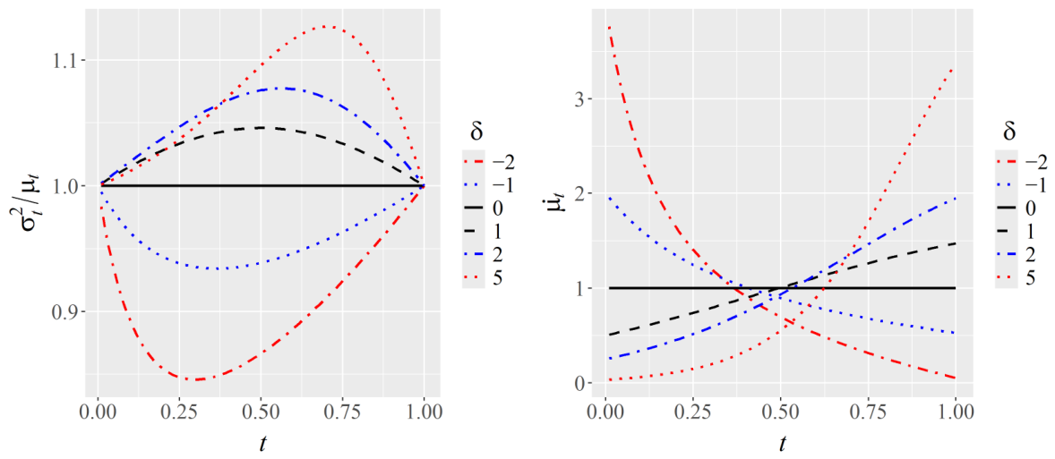
The left panel of Figure 1 displays the ratio ${\sigma }_t^2/{\mu }_t$ for an example where ${\lambda }_t=t$ and ${\delta }_t=\delta (t-1)$, with $\delta$ varying from −2 to 5 over the interval $t\in [0,1]$. Its right panel depicts the corresponding behavior of the rate of change ${\dot{\mu }}_t$ under the same linear specifications for ${\lambda }_t$ and ${\delta }_t$. As predicted by Equation (7), the direction of ${\dot{\mu }}_t$ depends on the sign of ${\dot{\delta }}_t$.

The Touchard marginal distribution can be interpreted as a weighted Poisson model, which connects the proposed framework with the broader class of weighted count distributions studied in the literature.

Proposition 1.

Model (1) belongs to the class of weighted Poisson processes [22,26,39,40,41].

Proof. 

Let $Y\left(t\right)\sim \mathrm{Poisson}\left({\lambda }_t\right)$ and define the weight function

$${\omega }_t\left(k\right)=exp\left({\lambda }_t\right){(k+1)}^{{\delta }_t},k\in \mathbb{N}.$$

Then

$$\begin{array}{cc}\hfill {\displaystyle \frac{{\omega }_t\left(k\right)P[Y\left(t\right)=k]}{E\left[{\omega }_t\left(Y\right)\right]}}& ={\displaystyle \frac{exp\left({\lambda }_t\right){(k+1)}^{{\delta }_t}exp(-{\lambda }_t){\lambda }_t^k/k!}{E[exp\left({\lambda }_t\right){(Y\left(t\right)+1)}^{{\delta }_t}]}}\hfill \\ \hfill & ={\displaystyle \frac{{\lambda }_t^k{(k+1)}^{{\delta }_t}}{k!\tau ({\lambda }_t,{\delta }_t)}}=p_k\left(t\right).\hfill \end{array}$$

(10)

Therefore, (1) can be represented as a weighted Poisson distribution, which proves the result.    □

Although Balakrishnan and Kozubowski [30] introduced a class of weighted Poisson processes with stationary and independent increments, the Touchard process does not belong to this class.

Proposition 2.

Let $X\left(t\right)$ be a Touchard process on the interval $[0,1]$ with parameters ${\lambda }_t$ and ${\delta }_t$. Then, except in the special case ${\delta }_t=0$, the process cannot admit a representation with stationary and independent increments.

Proof. 

Following Balakrishnan and Kozubowski [30], consider a hypothetical process $S\left(t\right)$ generated by stationary and independent increments with success probability proportional to t as $S\left(t\right)={\sum }_{i=1}^n{I}_i\left(t\right)$, where $\left\{I_i\left(t\right)\right\}$ is a random sample from a Bernoulli distribution with success probability t with n denoting a Touchard outcome in $[0,1]$, with parameters $\lambda ={\lambda }_1$ and $\delta ={\delta }_1$. Thus, given $X\left(1\right)=n$, the partial count $S\left(t\right)$ follows the Binomial form

$$\begin{array}{c}\hfill P[S\left(t\right)=k|X\left(1\right)=n]=\left({\displaystyle \genfrac{}{}{0pt}{}{n}{k}}\right)t^k{(1-t)}^{n-k},\end{array}$$

for $0\le k\le n$. Hence, the distribution of $S\left(t\right)$ is

$$\begin{array}{cc}\hfill P\left[S\right(t)=k]& =\sum _{n\ge k}P[S\left(t\right)=k|X\left(1\right)=n]·p_n\left(1\right)\hfill \\ \hfill & ={\displaystyle \frac{{(\lambda ·t)}^k}{k!}}·{\displaystyle \frac{T\left(\lambda \right(1-t),\delta ,k)}{T(\lambda ,\delta ,0)}},\hfill \end{array}$$

where

$$\begin{array}{c}\hfill T(\lambda ,\delta ,k)={\displaystyle \sum _{n^{\prime }=0}^{\infty }}{\displaystyle \frac{{\lambda }^{n^{\prime }}{(k+n^{\prime }+1)}^{\delta }}{n^{\prime }!}}.\end{array}$$

Therefore, the Touchard process outcome $X\left(1\right)$ cannot arise from stationary and independent increments, since the intermediate process $S\left(t\right)$ does not follow a Touchard distribution for $t\in [0,1]$, except in the special case $\delta =0$, corresponding to the Poisson process.    □

This implies that nonstationary and dependent increments must be considered. For a given time increment $\mathrm{\Delta }t>0$, we examine the interval $[0,t+\mathrm{\Delta }t]$ where $X(t+\mathrm{\Delta }t)\ge X\left(t\right)$. Because the subinterval $[t,t+\mathrm{\Delta }t]$ does not start at the origin, we represent the count within this subinterval as $X(t,\mathrm{\Delta }t)=X(t+\mathrm{\Delta }t)-X\left(t\right)$.

For a sufficiently small $\mathrm{\Delta }t$, $X(t,\mathrm{\Delta }t)$ becomes a dichotomous increment of the process, which we assume to be a Bernoulli distribution conditional on $X\left(t\right)$, as 

$$\begin{array}{cc}\hfill {\pi }_k(t+\mathrm{\Delta }t)& =P\left[X\right(t,\mathrm{\Delta }t)=1\mid X(t)=k],\hfill \end{array}$$

where ${\pi }_k(t+\mathrm{\Delta }t)$ is the increment probability from k at time t to $k+1$ at time $t+\mathrm{\Delta }t$, for $t\ge k\mathrm{\Delta }t$. This restriction follows from the sequential nature of the counting process, in which transitions between states occur incrementally. For example, reaching $k=2$ requires passing through $k=0$ and $k=1$, so the minimum time interval needed to reach $k=2$ is $2\mathrm{\Delta }t$.

We now establish the recursive conditional structure induced by the dependence of $X(t,\mathrm{\Delta }t)$ on both t and k, leading to an explicit expression for the transition probabilities ${\pi }_k(t+\mathrm{\Delta }t)$.

Proposition 3

(Recursive transition probabilities). Let $\left\{X\right(t\left)\right\}$ be a Touchard counting process with marginal probabilities $p_k\left(t\right)$ given by (1). For a sufficiently small $\mathrm{\Delta }t>0$, assume that the increment

$$X(t,\mathrm{\Delta }t)=X(t+\mathrm{\Delta }t)-X\left(t\right)$$

is dichotomous conditional on $X\left(t\right)=k$, with success probability

$${\pi }_k(t+\mathrm{\Delta }t)=P[X(t,\mathrm{\Delta }t)=1\mid X\left(t\right)=k].$$

Then, the transition probabilities are recursively given by

$$\begin{array}{c}\hfill {\pi }_0(t+\mathrm{\Delta }t)=1-{\displaystyle \frac{p_0(t+\mathrm{\Delta }t)}{p_0\left(t\right)}},\end{array}$$

(11)

and, for $k\ge 1$,

$$\begin{array}{c}\hfill {\pi }_k(t+\mathrm{\Delta }t)={\pi }_{k-1}(t+\mathrm{\Delta }t){\left({\displaystyle \frac{k}{k+1}}\right)}^{{\delta }_t}{\displaystyle \frac{k}{{\lambda }_t}}-{\displaystyle \frac{p_k(t+\mathrm{\Delta }t)-p_k\left(t\right)}{p_k\left(t\right)}}.\end{array}$$

(12)

Moreover, ${\pi }_k(t+\mathrm{\Delta }t)=0$ for $t<k\mathrm{\Delta }t$.

Proof. 

For $k=0$, the event $\left\{X\right(t+\mathrm{\Delta }t)=0\}$ occurs only when $X\left(t\right)=0$ and no increment occurs over $[t,t+\mathrm{\Delta }t]$. Hence,

$$\begin{array}{cc}\hfill p_0(t+\mathrm{\Delta }t)& =P\left[X\right(t+\mathrm{\Delta }t)=0]\hfill \\ \hfill & =P\left[X\right(t,\mathrm{\Delta }t)=0,X(t)=0]\hfill \\ \hfill & =[1-{\pi }_0(t+\mathrm{\Delta }t)]p_0\left(t\right),\hfill \end{array}$$

(13)

which yields (11).

For $k\ge 1$, the event $\left\{X\right(t+\mathrm{\Delta }t)=k\}$ can occur in two mutually exclusive ways: either the process was at state $k-1$ at time t and one event occurred, or it was already at state k and no event occurred. Therefore,

$$\begin{array}{cc}\hfill p_k(t+\mathrm{\Delta }t)& =P\left[X\right(t+\mathrm{\Delta }t)=k]\hfill \\ \hfill & =P\left[X\right(t,\mathrm{\Delta }t)=1,X(t)=k-1]+P\left[X\right(t,\mathrm{\Delta }t)=0,X(t)=k]\hfill \\ \hfill & ={\pi }_{k-1}(t+\mathrm{\Delta }t)p_{k-1}\left(t\right)+[1-{\pi }_k(t+\mathrm{\Delta }t)]p_k\left(t\right).\hfill \end{array}$$

(14)

Rearranging (14), we obtain

$$\begin{array}{cc}\hfill p_k(t+\mathrm{\Delta }t)-p_k\left(t\right)& ={\pi }_{k-1}(t+\mathrm{\Delta }t)p_{k-1}\left(t\right)-{\pi }_k(t+\mathrm{\Delta }t)p_k\left(t\right).\hfill \end{array}$$

Using (1), we have

$${\displaystyle \frac{p_{k-1}\left(t\right)}{p_k\left(t\right)}}={\left({\displaystyle \frac{k}{k+1}}\right)}^{{\delta }_t}{\displaystyle \frac{k}{{\lambda }_t}},$$

and therefore

$$\begin{array}{c}\hfill p_k(t+\mathrm{\Delta }t)-p_k\left(t\right)=\left\{{\pi }_{k-1}(t+\mathrm{\Delta }t){\left({\displaystyle \frac{k}{k+1}}\right)}^{{\delta }_t}{\displaystyle \frac{k}{{\lambda }_t}}-{\pi }_k(t+\mathrm{\Delta }t)\right\}{p}_k\left(t\right).\end{array}$$

Solving for ${\pi }_k(t+\mathrm{\Delta }t)$ gives (12). The condition ${\pi }_k(t+\mathrm{\Delta }t)=0$ for $t<k\mathrm{\Delta }t$ follows from the sequential nature of the counting process, since reaching state k requires at least k one-step increments.    □

Thus, the Touchard process is not defined only by requiring $X\left(t\right)$ to follow a Touchard distribution for each t, but by combining these marginal distributions with the recursively defined transition probabilities in (11) and (12). These recursive probabilities are valid Bernoulli probabilities provided that the marginal distributions at t and $t+\mathrm{\Delta }t$ satisfy conditions ensuring that ${\pi }_k(t+\mathrm{\Delta }t)\in [0,1]$. To see this, let $q_k(t,\mathrm{\Delta }t)={\pi }_k(t+\mathrm{\Delta }t)p_k\left(t\right)$ and $q_{-1}(t,\mathrm{\Delta }t)=0$. From (14), we have

$$q_k(t,\mathrm{\Delta }t)-q_{k-1}(t,\mathrm{\Delta }t)=p_k\left(t\right)-p_k(t+\mathrm{\Delta }t).$$

Summing this identity from $j=0$ to k yields

$$q_k(t,\mathrm{\Delta }t)={\displaystyle \sum _{j=0}^k}\{p_j\left(t\right)-p_j(t+\mathrm{\Delta }t)\}=F_t\left(k\right)-F_{t+\mathrm{\Delta }t}\left(k\right),$$

where $F_t\left(k\right)={\sum }_{j=0}^k{p}_j\left(t\right)$ denotes the distribution function of $X\left(t\right)$. Hence,

$${\pi }_k(t+\mathrm{\Delta }t)={\displaystyle \frac{F_t\left(k\right)-F_{t+\mathrm{\Delta }t}\left(k\right)}{p_k\left(t\right)}}.$$

Therefore, ${\pi }_k(t+\mathrm{\Delta }t)\in [0,1]$ whenever

$$0\le F_t\left(k\right)-F_{t+\mathrm{\Delta }t}\left(k\right)\le p_k\left(t\right),$$

or equivalently,

$$F_t(k-1)\le F_{t+\mathrm{\Delta }t}\left(k\right)\le F_t\left(k\right),k\ge 0,$$

with $F_t(-1)=0$. For sufficiently small $\mathrm{\Delta }t$, this condition is naturally expected in a counting-process construction with dichotomous increments, since probability mass can move at most one state to the right over the interval $[t,t+\mathrm{\Delta }t]$.

Following this construction, the recursive structure defined by (14) and (12), together with the marginal distributions specified in (1), yields a well-defined discrete-time formulation of the process. Notably, except when ${\lambda }_t=\lambda ·t$ and ${\delta }_t=0$ (corresponding to the homogeneous Poisson process), the Touchard process admits a representation as a weighted Poisson process with nonstationary and dependent increments.

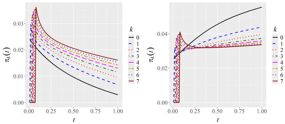
Figure 2 illustrates how transition probabilities can vary as a function of t and k for the cases of overdispersion (${\delta }_t<0$) and underdispersion (${\delta }_t>0$). In the overdispersion case, the probabilities decrease, starting from different increasing values at points $k\mathrm{\Delta }t$. In contrast, the shapes exhibit more varied patterns for underdispersion, except for ${\pi }_0(t+\mathrm{\Delta }t)$, which shows an increasing trend.

3. Simulations

Algorithm 1 provides a pseudo-code for simulating a Touchard process where ${\lambda }_t$ and ${\delta }_t$ are linear functions of time. This simulation can be performed straightforwardly using (11) and (12) with an appropriate choice of $\mathrm{\Delta }t$. To assess the sensitivity of the simulation algorithm to the discretization step size, we repeated the simulation with $\mathrm{\Delta }t=0.01$ and $\mathrm{\Delta }t=0.005$. The purpose of this comparison is to verify that the dichotomous-increment approximation remains stable as the time grid is refined. In practice, $\mathrm{\Delta }t$ should be chosen sufficiently small so that the transition probabilities ${\pi }_k(t+\mathrm{\Delta }t)$ remain within $[0,1]$ and the probability of more than one event within a single step is negligible.

The proposed Touchard process does not require specific functional forms for ${\lambda }_t$ and ${\delta }_t$. In this simulation study, linear specifications were adopted primarily for illustrative purposes and to facilitate interpretation of the resulting process dynamics. However, in practical applications, more flexible structures may be considered, including regression-type formulations involving covariates, seasonal effects, or smooth functions of time. Such extensions are consistent with previous developments on Touchard regression models and quasi-likelihood formulations for weighted Poisson distributions [26], and provide a natural direction for future research on nonstationary count processes.

Algorithm 1: Simulating a Touchard Process with time linear functions ${\lambda }_t$ and ${\delta }_t$

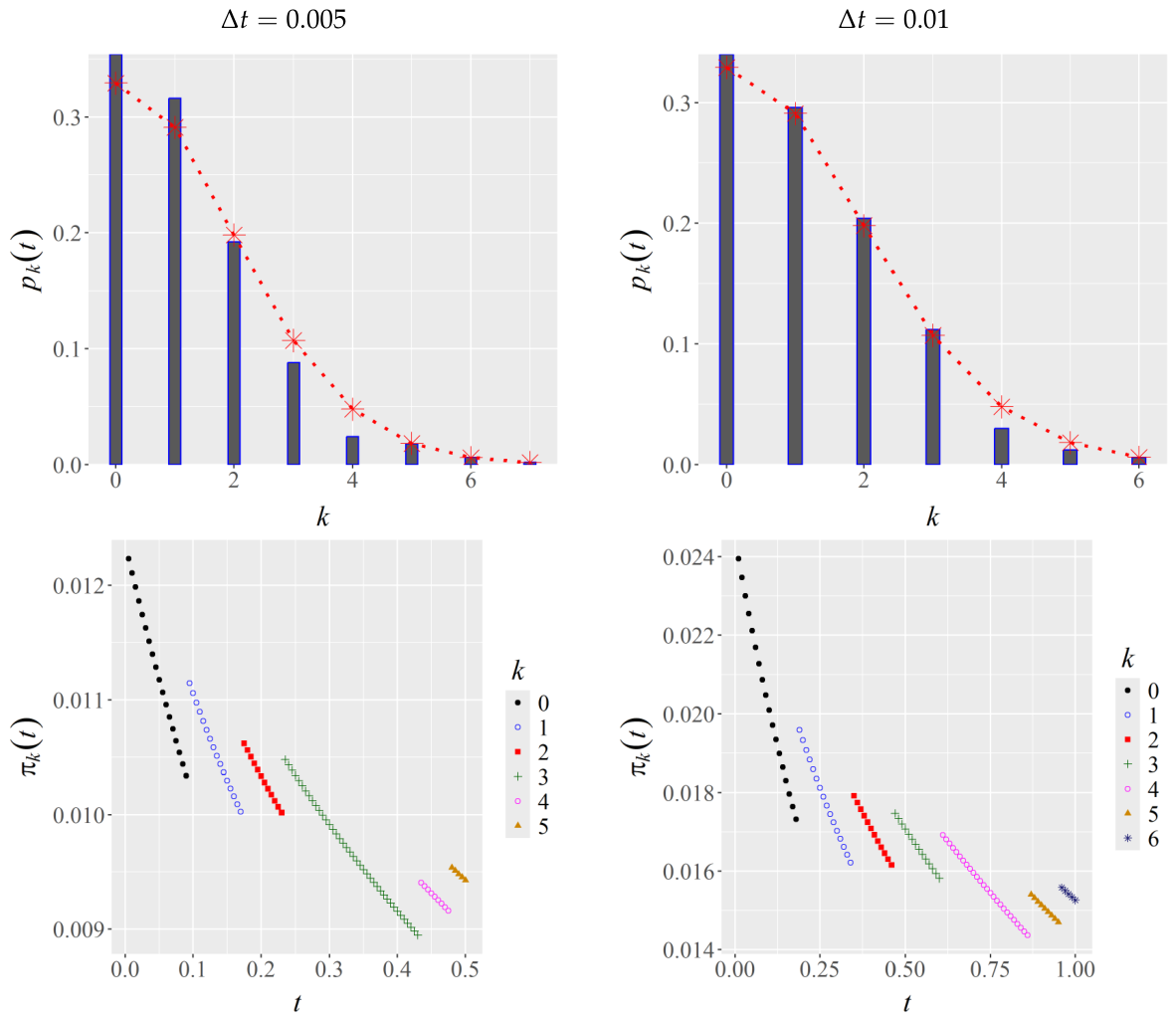
Figure 3 (top) presents the empirical frequency distributions obtained from 500 simulated realizations of the Touchard process with ${\lambda }_t=2.5t$ and ${\delta }_t=-1.5t$ over the interval $t\in [0,1]$, considering discretization steps $\mathrm{\Delta }t=0.01$ and $\mathrm{\Delta }t=0.005$. In both cases, the simulated frequencies agree well with the corresponding theoretical Touchard probabilities. This adherence is further supported by the likelihood ratio and chi-square goodness-of-fit tests, which produced p-values of 0.248 and 0.565 for $\mathrm{\Delta }t=0.01$, and 0.107 and 0.200 for $\mathrm{\Delta }t=0.005$, respectively. For both discretization schemes, the simulated terminal distributions remained stable and in good agreement with the target Touchard distribution, indicating that the choice $\mathrm{\Delta }t=0.01$ provides an adequate numerical discretization for the examples considered.

The bottom panel of Figure 3 illustrates the evolution of the transition probabilities associated with simulated trajectories resulting in the terminal outcome $X\left(1\right)=6$, for both $\mathrm{\Delta }t=0.005$ and $\mathrm{\Delta }t=0.01$. The figure highlights the discrete jump behavior of the recursively defined transition probabilities as functions of both the state k and time t. The R codes and functions used for simulating Touchard counts are openly available on Figshare (https://doi.org/10.6084/m9.figshare.27297291).

In practical applications, these jumps can be induced by events that naturally lead to a concentration of counts at specific moments. For example, in a stochastic process modeling individual customer arrivals at a store, there may be an increased probability of group arrivals, such as a family arriving by car. Similarly, traffic accident records can exhibit concentration at certain times due to inaccuracies in time recording, such as rounding. This latter case is discussed in detail in Section 5.

4. Parameter Estimation

The Touchard parametrization is identifiable at a fixed time t. Indeed,

$$\begin{array}{c}\hfill {\displaystyle \frac{p_{k+1}\left(t\right)}{p_k\left(t\right)}}={\displaystyle \frac{{\lambda }_t}{k+1}}{\left({\displaystyle \frac{k+2}{k+1}}\right)}^{{\delta }_t},\end{array}$$

so equality of the distributions for two parameter pairs implies equality of the corresponding successive probability ratios for all k, which is only possible if both ${\lambda }_t$ and ${\delta }_t$ coincide.

The Touchard process belongs to the exponential family, which is known for its advantageous inferential properties, including sufficient statistics, tractable likelihood functions, and maximum likelihood estimators that satisfy the usual regularity properties, such as consistency and asymptotic normality under standard conditions [42]. Given a random sample $x_1\left(t\right),\dots ,x_n\left(t\right)$ observed at a fixed time t, the resulting likelihood function is

$$\begin{array}{cc}\hfill L({\lambda }_t,{\delta }_t|\left\{x_i\left(t\right)\right\})& ={\left(\prod _i{x}_i\left(t\right)!\right)}^{-1}{\lambda }_t^{S_1\left(t\right)}exp\left\{{\delta }_t{S}_2\left(t\right)\right\}{\left[\tau ({\lambda }_t,{\delta }_t)\right]}^{-n},\hfill \end{array}$$

(15)

with sufficient statistics $S_1\left(t\right)={\sum }_i{x}_i\left(t\right)$ and $S_2\left(t\right)={\sum }_{i}ln(x_i\left(t\right)+1)$ by the factorization theorem. The first and second derivatives of $\tau ({\lambda }_t,{\delta }_t)$ with respect to ${\lambda }_t$ and ${\delta }_t$ are

$$\begin{array}{cc}\hfill {\displaystyle \frac{\mathsf{\partial }\tau ({\lambda }_t,{\delta }_t)}{\mathsf{\partial }{\lambda }_t}}& ={\displaystyle \frac{\tau ({\lambda }_t,{\delta }_t)}{{\lambda }_t}}·{\mu }_t,\hfill \\ \hfill {\displaystyle \frac{\mathsf{\partial }\tau ({\lambda }_t,{\delta }_t)}{\mathsf{\partial }{\delta }_t}}& =\tau ({\lambda }_t,{\delta }_t)E\{ln[X\left(t\right)+1]\},\hfill \end{array}$$

and

$$\begin{array}{cc}\hfill {\displaystyle \frac{{\mathsf{\partial }}^2\tau ({\lambda }_t,{\delta }_t)}{\mathsf{\partial }{\lambda }_t^2}}& =\tau ({\lambda }_t,{\delta }_t)·{\displaystyle \frac{E\left[X{\left(t\right)}^2\right]-{\mu }_t}{{\lambda }_t^2}},\hfill \\ \hfill {\displaystyle \frac{{\mathsf{\partial }}^2\tau ({\lambda }_t,{\delta }_t)}{\mathsf{\partial }{\delta }_t^2}}& =\tau ({\lambda }_t,{\delta }_t)E\left\{{ln}^2[X\left(t\right)+1]\right\},\hfill \\ \hfill {\displaystyle \frac{{\mathsf{\partial }}^2\tau ({\lambda }_t,{\delta }_t)}{\mathsf{\partial }{\delta }_t\mathsf{\partial }{\lambda }_t}}& ={\displaystyle \frac{\tau ({\lambda }_t,{\delta }_t)}{{\lambda }_t}}E\{Xln(X\left(t\right)+1)\}.\hfill \end{array}$$

Using these formulas, the maximization of the log-likelihood function $l({\lambda }_t,{\delta }_t)=lnL({\lambda }_t,{\delta }_t|\left\{x_i\left(t\right)\right\})$ at a given fixed t leads to the system of maximum likelihood equations

$$\begin{array}{c}\hfill \left\{\begin{array}{c}{S}_1\left(t\right)-n{\widehat{\mu }}_t=0,\hfill \\ S_2\left(t\right)-n\widehat{E}\{ln[X\left(t\right)+1]\}=0.\hfill \end{array}\right.\end{array}$$

(16)

Consequently, the maximum likelihood estimators (MLE) of ${\lambda }_t$ and ${\delta }_t$ are related to the moments estimators of ${\mu }_t$ and $E\{ln[X\left(t\right)+1\left]\right\}$. The Hessian matrix is

$$\begin{array}{cc}\hfill H\left(t\right)& =-\left[\begin{array}{cc}(n{\sigma }_t^2+S_1\left(t\right)-n{\mu }_t)/{\lambda }_t^2& n{\gamma }_t/{\lambda }_t\\ n{\gamma }_t/{\lambda }_t& nVar[ln(X\left(t\right)+1\left)\right]\end{array}\right],\hfill \end{array}$$

(17)

with ${\gamma }_t$ as defined in (8). However, rather than using (16) and (17), we prefer to maximize the log-likelihood function directly using Nelder–Mead’s method [43] implemented in R’s optim function. The R codes and functions for estimating Touchard parameters are available on Figshare (https://doi.org/10.6084/m9.figshare.27297291).

5. Motor Vehicle Crashes Data

The purpose of this section is to illustrate the practical implications of the Touchard process and to assess its ability to capture key empirical features of count data. The analysis focuses on the descriptive performance of the model, highlighting its flexibility in accommodating overdispersion and temporal variation, with the Poisson model serving as a natural benchmark.

We use motor vehicle crash data collected from the New York State Open Data Portal (https://data.ny.gov, USA; accessed on 29 August 2025) for this analysis. The dataset includes the number of motor vehicles involved per crash, as recorded in reports submitted to the New York State Department of Motor Vehicles by drivers and police agencies from 2018 to 2022. Among the four most densely populated counties in New York State (New York County, Kings, Bronx, and Queens), Queens and Kings had the highest rates of car accidents (

Table 1. Total number of crash reports observed in the four most densely populated counties of New York State from 2018 to 2022.

County	Total of Crash Reports
Queens	174,796
Kings	163,222
Bronx	96,985
New York	89,484

). This section presents the results of daily crashes registered in these two counties.

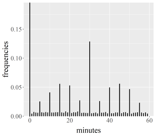
Our study considers time windows t ranging from 5 to 60 min in 5-min increments starting at 6:00 p.m., with a sample size of 1826 days. Figure 4 illustrates how the reported times are concentrated at specific minutes between 6:00 p.m. and 6:59 p.m., potentially due to rounding or uncertainty about the exact time of the accident. Consequently, it is reasonable to expect that the probability of recording an accident will show peaks at certain times, as in Figure 3 (right).

Table 2. Maximum likelihood estimates of the Touchard process parameters for the number of crashes observed in Queens County, New York, 2018–2022, together with the corresponding Bayesian Information Criterion (BIC) values for the Touchard, Poisson, zero-inflated Poisson (ZIP), and zero-inflated negative binomial (ZINB) models.

							BIC
t	$\widehat{\mathbf{\lambda }}$	s.e. ($\widehat{\mathbf{\lambda }}$)	$\widehat{\mathit{\delta }}$	s.e. ($\widehat{\mathit{\delta }}$)	${\widehat{\mathit{\mu }}}_t$	${\widehat{\mathit{\sigma }}}_{\mathbf{t}}^{\mathbf{2}}$	Touchard	Poisson	ZIP	ZINB
5	2.49	0.143	−1.23	0.143	1.5	2.00	5957.3	6018.8	5973.7	5964.0
10	2.87	0.143	−1.20	0.135	1.9	2.44	6410.3	6475.2	6428.3	6417.0
15	3.36	0.145	−1.19	0.130	2.3	2.99	6878.7	6947.4	6897.9	6886.4
20	3.96	0.152	−1.33	0.126	2.7	3.68	7288.9	7379.9	7324.2	7292.5
25	4.21	0.153	−1.31	0.126	3.0	4.00	7475.0	7561.6	7511.4	7478.0
30	5.63	0.168	−1.67	0.123	3.9	5.82	8201.0	8343.1	8306.0	8188.4
35	5.88	0.170	−1.69	0.125	4.1	6.19	8325.3	8464.8	8435.9	8307.0
40	6.52	0.176	−1.87	0.124	4.5	7.03	8574.6	8743.1	8715.3	8716.3
45	7.19	0.181	−2.06	0.124	4.9	7.96	8818.5	9020.6	8993.6	8989.6
50	7.74	0.186	−2.20	0.124	5.3	8.78	9008.7	9230.7	9208.3	9202.9
55	7.97	0.188	−2.22	0.126	5.5	9.04	9075.5	9293.0	9271.3	9263.0
60	10.02	0.200	−2.86	0.122	6.6	12.31	9673.5	10,018.1	10,002.6	9982.1

and

Table 3. Maximum likelihood estimates of the Touchard process parameters for the number of crashes observed in Kings County, New York, 2018–2022, together with the corresponding Bayesian Information Criterion (BIC) values for the Touchard, Poisson, zero-inflated Poisson (ZIP), and zero-inflated negative binomial (ZINB) models.

							BIC
t	$\widehat{\mathbf{\lambda }}$	s.e. ($\widehat{\mathbf{\lambda }}$)	$\widehat{\mathit{\delta }}$	s.e. ($\widehat{\mathit{\delta }}$)	${\widehat{\mathit{\mu }}}_{\mathbf{t}}$	${\widehat{\mathit{\sigma }}}_{\mathbf{t}}^{\mathbf{2}}$	Touchard	Poisson	ZIP	ZINB
5	1.54	0.119	−0.64	0.169	1.2	1.31	5202.4	5208.9	5204.9	5209.9
10	1.99	0.124	−0.70	0.151	1.5	1.73	5803.7	5816.5	5806.9	5811.9
15	2.48	0.129	−0.71	0.142	1.9	2.32	6377.6	6394.2	6390.8	6378.7
20	3.03	0.136	−0.79	0.137	2.4	2.93	6858.8	6882.6	6882.4	6854.4
25	3.40	0.141	−0.86	0.135	2.6	3.34	7120.5	7150.6	7148.6	7113.9
30	4.48	0.155	−1.13	0.132	3.4	4.58	7748.7	7805.8	7805.2	7733.1
35	4.85	0.160	−1.22	0.133	3.7	5.06	7940.5	8005.6	8008.9	8016.4
40	5.33	0.166	−1.27	0.136	4.1	5.67	8173.2	8240.2	8245.8	8253.3
45	5.98	0.174	−1.46	0.135	4.5	6.47	8428.3	8517.2	8522.0	8527.6
50	6.48	0.180	−1.55	0.138	4.8	7.13	8617.4	8712.9	8717.5	8725.0
55	6.86	0.184	−1.66	0.138	5.1	7.61	8746.5	8853.6	8859.2	8866.7
60	8.30	0.197	−2.09	0.138	6.0	9.68	9207.5	9367.2	9371.2	9378.7

present the maximum likelihood estimates (MLE) of the Touchard process parameters, their standard errors (s.e.), the sample mean, and the sample variance of the daily number of crashes. The smallest absolute ratio between the estimate and its standard error was 17.43 for ${\lambda }_5$ and 8.63 for ${\delta }_5$ (Queens), and 12.97 for ${\lambda }_5$ and 3.81 for ${\delta }_5$ (Kings). Using the asymptotic normality property of the MLEs, we find that all parameter estimates are highly statistically significant (p-values $<{10}^{-4}$).

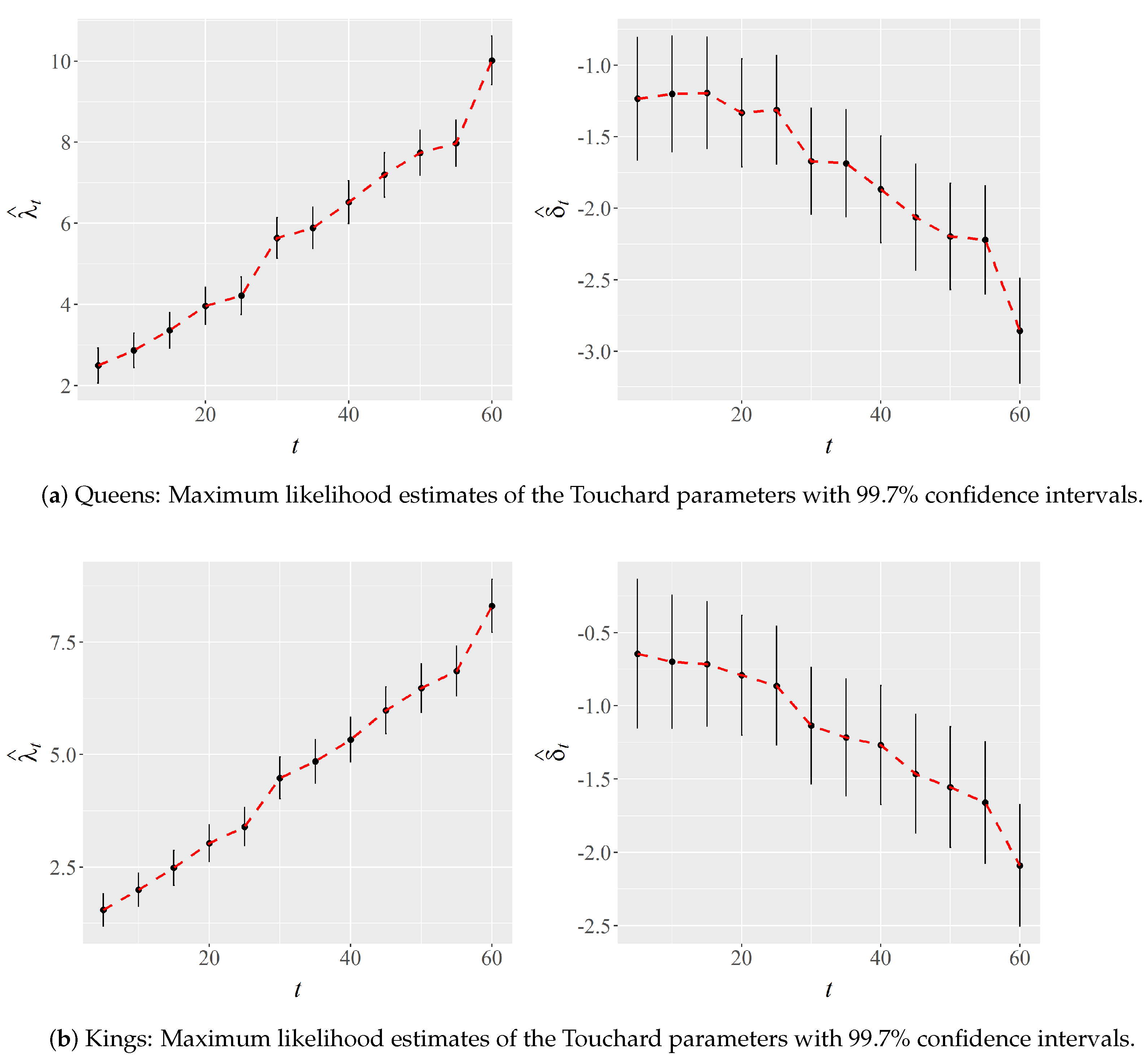
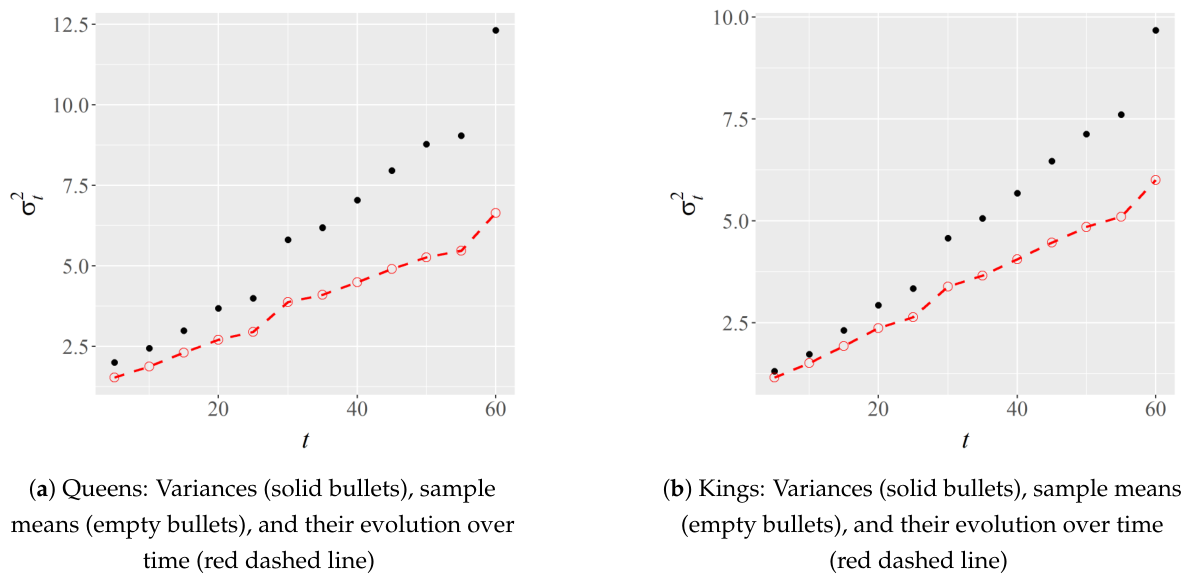
Furthermore, comparisons based on the Bayesian Information Criterion (BIC) indicate that the Touchard model generally provided a better fit than the Poisson and zero-inflated Poisson (ZIP) models, while remaining competitive with the zero-inflated negative binomial (ZINB) model across the aggregation intervals considered. Figure 5 illustrates the MLEs and their 99.7% confidence intervals. The sample variances exceeded the mean values for all t intervals, indicating overdispersion relative to the Poisson distribution (Table 2 and Table 3 and Figure 6).

Figure 7 and Figure 8 show the daily empirical distributions of crashes (bars) together with the corresponding expected frequencies under the Touchard model (∗). The fitted distributions exhibit good agreement with the observed data, reflecting the greater flexibility of the Touchard process relative to the classical Poisson process.

The estimated parameters also provide useful insights into the crash-count dynamics across different aggregation windows. As the observation interval t increases, the estimated values of ${\lambda }_t$ increase steadily in both counties, reflecting the higher expected number of crashes accumulated over longer time periods. At the same time, the estimated values of ${\delta }_t$ become progressively more negative, indicating increasing departures from the equidispersion structure associated with the classical Poisson process. This behavior is consistent with the observed growth of the empirical variances relative to the means, suggesting that wider aggregation windows introduce additional heterogeneity and variability into the crash-count process. Overall, the estimated Touchard parameters capture both the evolving crash intensity and the changing dispersion structure of the data, highlighting the flexibility of the proposed process for modeling complex count dynamics.

The distribution of reported accident times by minute also suggests the presence of temporal concentration effects in the recording process. As illustrated in Figure 4, accident reports exhibit noticeable spikes at specific minute values, particularly at rounded or salient times such as 0, 15, 20, 30, and 45 min. This pattern may reflect reporting-time clustering or rounding effects commonly observed in administrative datasets. Such temporal concentration mechanisms may contribute to additional variability and departures from the equidispersion assumption underlying the classical Poisson process, thereby partially explaining the improved performance of the Touchard process relative to the Poisson benchmark in the empirical analysis.

6. Conclusions

The Touchard process, derived as a two-parameter extension of the classical Poisson process, provides a flexible and robust framework for modeling count data that exhibit non-Poisson characteristics, such as overdispersion, underdispersion, and temporal dependencies. By leveraging the Touchard probability distribution, this model captures the complex dynamics often observed in real-world scenarios that traditional Poisson models fail to adequately capture. Our study illustrates the practical applicability of the Touchard process by analyzing traffic accident data from Queens and Kings Counties, where the proposed model showed performance that was competitive with or superior to the alternative count models considered, depending on the aggregation interval. The empirical comparisons in this study focused on the Poisson model and zero-inflated variants to assess departures from the canonical Poisson process and account for excess zeros in the observed crash counts. Other flexible count models, including the Negative Binomial and COM-Poisson distributions, also represent relevant competing alternatives.

Key findings include the effective use of maximum likelihood estimation for parameter inference and an algorithm for simulating the Touchard process that highlights the evolution of transition probabilities. These components reinforce the practicality of the Touchard process for real-world data analysis, providing insights into phenomena involving temporal fluctuations and irregular event counts.

Further developments could focus on extending the current model by explicitly modeling the parameters ${\lambda }_t$ and ${\delta }_t$ as functions of covariates, enabling the Touchard process to capture more complex dependencies and provide a richer interpretation of the data. Exploring time-varying structures for ${\lambda }_t$ and ${\delta }_t$ could also yield more precise modeling of processes in which the event rate and dispersion change dynamically over time. In addition, while the present estimation framework considers random samples observed at a fixed time point, an important extension would be parameter inference from a single observed trajectory of the Touchard process over multiple time points, requiring likelihood constructions that explicitly account for the dependence induced by the recursive transition probabilities. These enhancements would broaden the applicability of the Touchard process, making it an even more versatile tool for analyzing non-Poisson count data across various fields.