Geometric Structure of Genomes Across the Tree of Life: Toward a Geometric Theory of Sequence Structure

Abstract

This work develops a geometric and statistical framework for analyzing the structure of biological sequences and explores its implications for understanding the emergence and evolution of life. Motivated by questions concerning the transition from prebiotic chemistry to living systems, the quantification of negentropy in organic matter, and the distinction between random and biologically viable sequences, we introduce mathematical descriptors that measure deviation from linearity and related geometric irregularities of self-replicating macromolecules. These descriptors reveal a pronounced geometric separation between biological DNA and random sequences, underscoring the non-random structural organization characteristic of living systems. Using these descriptors, we compare a broad range of species across the Tree of Life and examine how geometric complexity varies between primitive and more advanced organisms. We further investigate whether these measures provide a natural way to compare organismal complexity, characterize the structure of viable sequence space, and identify potential constraints on evolutionary trajectories. The framework also offers an initial perspective on how natural selection and stochastic mutations may jointly influence genomic organization. Finally, we outline speculative connections between increasing geometric irregularity and the emergence of biological complexity, suggesting that such geometric transitions may offer insight into the origins of life and the theoretical limits of evolutionary development.

1. Introduction

The origin of life and the mechanisms that shaped early evolution remain among the most challenging and conceptually profound questions in science (for classic overviews, see [1,2,3,4,5,6,7,8,9,10,11,12,13,14,15,16,17,18,19,20,21,22]). Despite extensive research across chemistry, biology, geology, and physics, many aspects of life’s emergence are inaccessible to direct observation, and competing theories often coexist without the possibility of decisive empirical resolution. This is not surprising: the relevant events occurred billions of years ago under environmental conditions that can only be partially reconstructed, and the available evidence is fragmentary, indirect, and shaped by subsequent geological processes. Even seemingly simple questions, such as the precise timing of life’s appearance on Earth, admit uncertainties of hundreds of millions of years, reflecting both the incompleteness of the fossil record and the difficulty of interpreting ancient geochemical signatures.

These limitations do not imply that progress is impossible but, rather, that fully deterministic or experimentally reproducible theories of life’s origin are unlikely to be achieved. Instead, conceptual frameworks that identify structural, informational, or geometric constraints on viable biological organization may offer a productive way forward. Such approaches aim not to reconstruct specific historical events but to characterize the quantitative properties that distinguish living systems from random chemistry and that shape the space of possible evolutionary trajectories. Within this perspective, mathematical structures and quantitative descriptors can play a central role in clarifying what kinds of molecular organization are compatible with replication, heredity, and functional diversification.

Given the inherent difficulties in formulating a complete and experimentally verifiable theory of the origin of life and early evolution, any meaningful conceptual framework must satisfy several broad criteria.

• Proposed scenarios should be consistent with physical and chemical plausibility, avoiding assumptions that contradict established principles;
• They must agree with the available empirical evidence, however fragmentary, including geological, biochemical, and genomic data;
• Finally, the underlying hypotheses should be logically coherent and grounded in general principles rather than relying exclusively on isolated or incomplete observations.

These criteria reflect the methodological constraints of origins-of-life research, where direct experimentation under ancient Earth conditions is impossible and the surviving evidence is sparse. At the same time, they highlight the increasing role of mathematics and computation in biological inquiry. Over the past decades, fields such as mathematical biology, theoretical biology, computational biology, and bioinformatics have emerged precisely to address questions that cannot be resolved through empirical observation alone. Mathematical models and computational analyses have provided insight into diverse biological phenomena, from molecular organization to evolutionary dynamics, by identifying structural patterns and constraints that are not accessible through traditional experimental approaches. Within this conceptual landscape, several fundamental questions arise concerning the quantitative structure of biological sequences and the constraints that govern their organization and evolution. Among them are the following:

• What quantitative characteristics must be satisfied for a transition from prebiotic chemistry to self-replicating, living systems?
• How can one measure the negentropy of individual organisms, groups of organisms, or living systems as a whole?
• To what extent do biological sequences differ from random sequences, and what structural features account for these differences?
• Can quantitative parameters distinguish primitive from more complex organisms, and do they provide a meaningful basis for comparing biological complexity?
• Is there a mathematical structure that naturally represents the DNA sequence of each organism and unifies all such sequences within a common framework?
• What are the properties of this structure; how does it evolve; and what theoretical limits, if any, constrain further evolutionary development?

Some of these questions have been explored in earlier work [23,24,25], where mathematical constructs and computational experiments were introduced to analyze the geometry of DNA sequences. Traditional approaches to biosequence analysis often rely on combinatorial methods such as pattern matching and combinatorics on words. In contrast, the present work adopts a geometric perspective, applying the idea of string geometrization to genomic sequences. A central contribution of this work is the introduction of a new geometric technique for the analysis of genomic sequences based on the representation of DNA sequences as monotone paths and monotone graphs. This framework provides quantitative descriptors, such as geometric deviation and path-based negentropy, that are not available through existing combinatorial or statistical methods. Because these constructions are general and reusable, they offer a methodological foundation that can support future studies of genomic organization, complexity, and the structure of viable sequence space.

Although modern molecular biology routinely analyzes DNA, RNA, and protein sequences, it remains a fundamental biological fact that all cellular organisms—bacteria, archaea, protists, fungi, plants, and animals—possess DNA-based genomes. RNA genomes occur exclusively in viruses, which are non-cellular entities with extremely small genomes and replication mechanisms that differ profoundly from those of cellular life. Because the present study aims to compare genomic organization across species in the biological sense, our analysis is restricted to cellular organisms, for which DNA is the universal hereditary substrate. Including RNA viruses would conflate cellular and non-cellular systems, introduce orders-of-magnitude differences in genome size, and require distinct methodological assumptions and scaling frameworks. Our focus on DNA genomes is therefore a deliberate and biologically coherent choice that ensures comparability across the Tree of Life. While RNA and protein analyses are essential in many modern contexts, such as transcriptomics, regulatory biology, and structural studies, they address questions different from those considered here. The geometric properties investigated in this work pertain specifically to large-scale organization of genomic DNA; extending these methods to viral RNA genomes would constitute a separate line of inquiry with its own biological and methodological constraints.

In developing this framework, we conducted a series of computational experiments on diverse genomic sequences, examining their geometric, structural, and statistical properties. The patterns observed in these analyses motivate several hypotheses and suggest possible interpretations of the underlying mechanisms that shape genomic organization. These interpretations are not presented as definitive conclusions but as informed conjectures grounded in computational evidence and guided by theoretical considerations. Their purpose is to stimulate further investigation and to highlight potential connections between geometric descriptors of sequences and broader questions concerning the emergence, structure, and evolution of living systems.

The remainder of this work is organized as follows. Section 2 introduces the basic notions and notation used throughout the paper. Section 3 recalls key definitions related to string geometrization and presents several new concepts, including the discrete irregular helix, the monotone graph, and measures of negentropy for monotone paths and monotone graphs; we also examine fundamental properties of these structures. Section 4 introduces the DNA Graph of Life and discusses how the proposed mathematical framework can be applied to its analysis. Section 5 defines the negentropy of individual species, groups of species, and the DNA Graph of Life as a whole. Section 6 describes, in detail, the computational procedures used in our experiments, and Section 7 presents the principal results obtained from these computations. In particular, we explore distinctions between biological and random sequences, potential boundaries of life expressed through the introduced geometric parameters, and gradients between primitive and complex organisms. Section 8 offers hypotheses and biological interpretations derived from our findings, while Section 9 outlines a speculative outlook concerning transitional states and the emergence of biological complexity. Section 10 concludes with final remarks and directions for future research.

Throughout the paper, selected key conclusions are highlighted for clarity. Several theoretical results related to string geometrization were previously stated without proof; the corresponding proofs are provided in Appendix A. Appendix B contains tables summarizing selected outcomes of our computational experiments.

2. Notions and Notation

2.1. General

$\left|X\right|$ denotes the cardinality of a set X, and $\overline{xy}$ denotes a straight line segment with endpoints x and y. $d(x,y)=\left|\right|x-y\left|\right|$ denotes the Euclidean distance between points x and y, and $d(x,Y)={inf}_{y\in Y}\left\{d(x,y)\right\}$ denotes the distance between point x and set Y.

Given a list T of non-negative real numbers $t_1,t_2,\dots ,t_k$, not all of which equal 0, a normalization of T is obtained by multiplying each value in T by ${\displaystyle \frac{100}{t_{max}}}$, where $t_{max}={max}_{1\le i\le k}\left\{t_i\right\}$.

Given an approximation algorithm A for a minimization problem $\Pi$ with a set of instances $D_{\Pi }$, let $A\left(I\right)$ be the value of an approximate solution on instance $I\in D_{\Pi }$ found by A. The approximation ratio of A on I is $R_A\left(I\right)={\displaystyle \frac{A\left(I\right)}{Opt\left(I\right)}}$, where $Opt\left(I\right)$ is the optimal solution for I; the worst-case performance ratio of A is $R_A=sup\{R_A\left(I\right):I\in D_{\Pi }\}$. We will say that an algorithm with performance ratio r finds an r-approximation to the optimal solution. For more details, the reader is referred to [26,27].

2.2. Notions of Theory of Words

The theory of words studies the structural properties of strings composed of letters of a given alphabet and provides algorithms for solving diverse problems defined on strings. Among the most important motivations for the discipline is its relevance to computational biology and, more precisely, to the automated analysis of biosequences. This includes a great variety of problems whose portrayal is beyond the purposes of the present paper. Some avenues of the ongoing research are surveyed in [28,29,30,31,32,33,34].

In the literature, the terms word, sequence, and string are often used interchangeably. A sequence is often defined in mathematics as a function whose domain consists of a set of consecutive integers, and a string over X, where X is a finite set, is often defined as a finite sequence s of elements from X (X is also sometimes called the alphabet). The term word is frequently used as an abstraction of the other two terms. In biology, the prevalent term is biosequence; the DNA sequences that are the subject of our interest in the present work are built from the four letters A, T, C, and G and have finite lengths.

Below, we recall a few basic notions and fix some notations to be used in this paper.

In the string $s=s_1\dots s_m$ over set X, $s_i$ is the $i^{\mathrm{th}}$ term of s ($1\le i\le m$), which is some element of X. The number of elements in s is called the length of s and denoted as $\left|s\right|$. If $\left|s\right|=0$, we say that s is the empty string, denoted by $\lambda$. By $x^k$ we denote $k\ge 1$ consecutive repetitions of term x in string s.

A $substring$ of a string s is obtained by selecting some or all consecutive elements of s. More formally, a string v is a substring of a string s if there are strings u and w such that $s=uvw$ (where we may have $u=\lambda$ or $v=\lambda$).

2.3. Notions of Graph Theory

Let $G(V,E)$ be a simple graph, i.e., without multiple edges between any pair of vertices and with no loops (edges that connect a vertex to itself). A simple path in G is a sequence of vertices of G such that no vertex is repeated. A shortest path between two vertices of G is a simple path of a minimum length (number of edges) connecting the vertices. A simple cycle is a closed simple path. G is triangle-free if it contains no triangle, i.e., a cycle of length 3. G is connected if there is a path of edges of G between any two of its vertices. G is sparse if $\left|E\right|=O\left(\right|V\left|\right)$; otherwise, it is dense. G is bipartite if its vertices can be divided into two parts such that the graph edges can connect vertices only from different parts but not from the same part. A graph is bipartite if and only if it is two-colorable (i.e., its vertices can be colored by only two colors so that any two adjacent vertices are colored by different colors).

Graph G is geometric if its vertices are points of ${\mathbb{R}}^n$ and its edges are segments containing graph vertices. A geometric graph G is rectilinear if each edge of G is a straight line segment that is parallel to a coordinate axis.

A graph is called directed if its edges have directions. A directed path in a directed graph is a sequence of vertices such that for each vertex v in the sequence, there is a directed edge pointing to a successor of v in the sequence. A directed graph is connected if there is a directed path between any two vertices. A directed graph is strongly connected if, for any pair of vertices (u, v), there is a directed path from u to v and a directed path from v to u.

3. Theoretical Background: String Geometrization, Monotone Paths, Monotone Graphs, and Negentropy

3.1. Monotone Paths

In order to make the paper self-contained, in this section, we first recall some basic definitions and related properties from [23,24,25]. Then, we extend those considerations by introducing new structures and concepts to be used in DNA sequence interpretation.

Let $\theta$ be the origin of the Cartesian coordinate system. A monotone path in ${\mathbb{Z}}_{+}^n$ is a sequence of points (nodes) $a_0=\theta ,a_1,a_2,\dots ,a_m\in {\mathbb{Z}}_{+}^n$, connected by segments that are unit edges of the rectangular grid, where the coordinates of any point $a_i$, $i\ge 2$, are pairwise greater than or equal to the corresponding coordinates of any preceding point.

Let $L=q_0\dots q_m$, $q_0=\theta$ be a monotone path of length m. The segment $\overline{q_0{q}_m}$ is determined by the total composition of the string. It is the “ideal” (or “average”) direction of the path determined by base composition and stands for linearity. The actual path L fluctuates around that line. $d(q_i,\overline{q_0{q}_m})$ measures how much the partial composition at position i deviates from the final composition “direction” determined by the segment $\overline{q_0{q}_m}$, i.e., how much it deviates from linearity.

Let $L=q_0\dots q_m$ be a monotone path of length m. If, for every node q of L, the voxel centered at q intersects the line segment $\overline{\theta p}$, then we say that L is a linear path or, equivalently, that L exhibits linearity. In the degenerate case where a monotone path is aligned with one of the coordinate axes, L is called an inline path.

It is easy to see that the following facts hold:

Fact 1.

Given a point $p\in {\mathbb{Z}}_{+}^n$, there is at least one linear path from θ to p.

Fact 2.

If L is a linear path from θ to p, then $d(q,\overline{\theta p})\le {\displaystyle \frac{\sqrt{n}}{2}}$$\forall q\in L$.

Remark 1.

Note that when $n=4$ (which is the case for DNA sequences), the $adv$ and $mdv$ of a linear string are, at most, 1.

We define the maximum deviation from linearity of L as

$$mdv\left(L\right)={\displaystyle \underset{i=0}{\overset{m}{max}}}\left\{d(q_i,\overline{q_0{q}_m})\right\},$$

(1)

and the average deviation from linearity of L as

$$adv\left(s\right)={\displaystyle \frac{{\sum }_{i=0}^{m}d(q_i,\overline{q_0{q}_m})}{m+1}}.$$

(2)

These two characteristics will play a crucial role in our experiments and in interpreting the results we obtain.

The third characteristic of a string s will be called the number of local maxima of s and is denoted as $nlm\left(s\right)$. Commonly, by a local maximum one means a point $q_i\in L$ for which $d(q_i,\overline{q_0{q}_m})$ is greater than $d(q_{i-1},\overline{q_0{q}_m})$ and $d(q_{i+1},\overline{q_0{q}_m})$. However, regarding the usual applications of extrema of discrete functions—in particular, in view of our own purposes—counting all such maxima does not seem to be very relevant. Instead, local maxima can be counted only if they “stand out" compared to other, “indistinguishable” local extrema, which differ very little from neighboring points. Thus, we adopt the notion of the number of local maxima as “method-dependent”. Specifically, our choice of method is MATLAB’s peakfinder function provided in [35]. This is a computational method for identifying local maxima in a numerical sequence by evaluating changes in slope or curvature under specified thresholds. It defines a peak as a local extremum that exceeds its neighbors by at least a threshold (named sel), which is user-specified or designated by default. The algorithm isolates local maxima whose values exceed their neighbors according to that criterion. More specifically, the algorithm maintains two running values: $mx$, which is the highest value found since the last minimum, and $mn$, which is the lowest value found since the last maximum. These values are updated constantly as the function rises and falls. A minimum is recorded whenever the signal switches from falling to rising, and a peak is accepted only if $mx-mn\ge \mathtt{sel}$.

Let $p=(p_1,\dots ,p_n)$ be a point in ${\mathbb{Z}}_{+}^n$. Let ${\mathbb{H}}_p$ be the set of all monotone discrete paths between $\theta$ and p. It is easy to see that the following holds.

Fact 3.

$|{\mathbb{H}}_p|={\displaystyle \frac{(p_1+\dots +p_n)!}{p_1!\dots p_n!}}$.

Each path $L\in {\mathbb{H}}_p$ consists of $1+{\sum }_{i=1}^m{p}_i$ points, with the initial point denoted as $\theta$ and the terminal point denotes as p. Now, let $\mathbb{H}\left(m\right)$ be the set of all monotone paths of length m. Then, we have

Fact 4.

$\mathbb{H}\left(m\right)={\bigcup }_p{\mathbb{H}}_p$, where $p_1+\cdots +p_n=m$.

3.2. String Geometrization

Let $s=s_1\cdots s_m$ be a string on an alphabet $X=\{x_1,x_2,\dots ,x_n\}$. We inductively construct an ordered set $L\left(s\right)$ of points $q_0=\theta ,q_1,\dots ,q_m$ corresponding to string s as follows.

Let $q_i=(q_{i,1},\dots ,q_{i,n})$ be the $i^{\mathrm{th}}$ element of $L\left(s\right)$ for $0\le i<m$. If $s_{i+1}=x_j$ for some j, $1\le j\le n$, then we set $q_{i+1}=(q_{i,1},\dots ,q_{i,j}+1,\dots ,q_{i,n})$. Thus, we obtain a monotone discrete path $L\left(s\right)$ with $\left|L\right(s\left)\right|=\left|s\right|=m+1$ associated with string s, in which the coordinates of a point are pairwise greater than or equal to the corresponding coordinates of any preceding point. 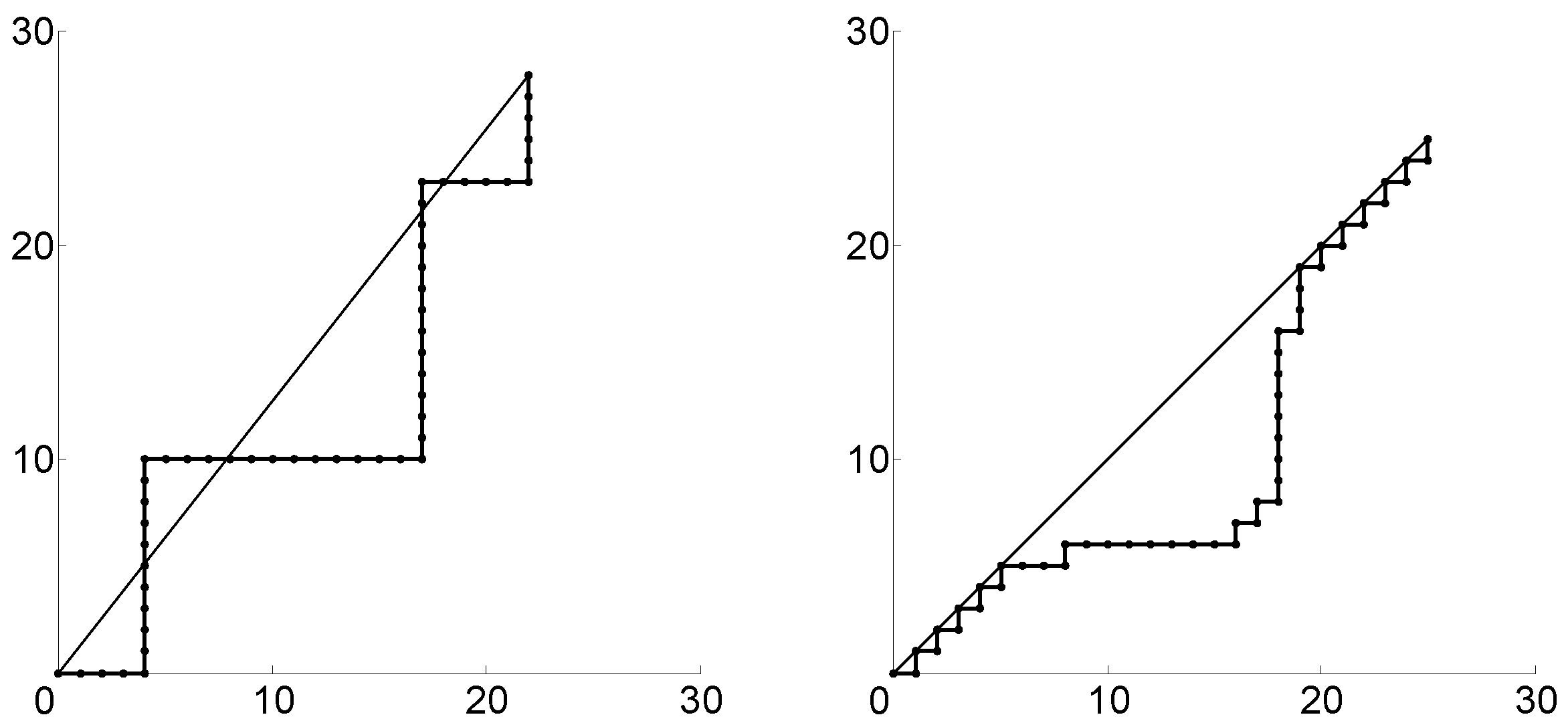Figure 1 (left) gives an example of a string over the alphabet $\{x,y\}$ and its corresponding monotone discrete path.

With reference to Formulas (1) and (2), we can define the maximum deviation from linearity and average deviation from linearity of s as $mdv\left(s\right)=mdv\left(L\right(s\left)\right)$ and $adv\left(s\right)=adv\left(L\right(s\left)\right)$. We call s a linear string if its corresponding monotone path $L\left(s\right)$ is linear. If $L\left(s\right)$ is inline, then s is an inline string.

Denote by $ma{x}_{mdv}\left(s\right)$ the greatest $mdv$ attained by a permutation of string s, i.e., 

$$ma{x}_{mdv}\left(s\right)=max\{mdv\left(s^{\prime }\right):s^{\prime }\mathrm{is}\mathrm{a}\mathrm{permutation}\mathrm{of}s\}.$$

The following theorem (stated in [23] without proof) will be used in Section 4 in the deliberation on “borders of life”. The proof of the theorem is given in Appendix A.

Theorem 1.

Given a string s over an alphabet $X=\{x_1,\dots ,x_n\}$ in which letter $x_i$ appears $a_i$ times, $1\le i\le n$,

$$\underset{mdv}{max}\left(s\right)=\underset{\mathbb{P}}{max}\left\{\sqrt{{\displaystyle \frac{\left({\sum }_{i\in N}{a}_i^2\right)\left({\sum }_{j\in Z}{a}_j^2\right)}{{\sum }_{k=1}^n{a}_k^2}}}\right\},$$

(3)

where $\mathbb{P}$ is the set of all partitions of $\{1,2,\dots ,n\}$ into two disjoint, nonempty sets N and Z.

If $P=\{N^{*},Z^{*}\}\in \mathbb{P}$ is a partition for which ${max}_{mdv}\left(s\right)$ is attained, then for every permutation $s^{\prime }$ of s, the corresponding discrete monotone path contains the point expressed as $p=(p_1,p_2,\dots ,p_n)$, where $p_i=a_i$ if $i\in N^{*}$ and $p_i=0$ if $i\in Z^{*}$, $mdv\left(s^{\prime }\right)={max}_{mdv}\left(s^{\prime }\right)$.

Remark 2.

Given a string s of length m, the numbers $a_1,\dots ,a_n$ of appearances of the letters $x_1,\dots ,x_n$ can be counted with $O\left(m\right)$ operations. Once this is done, ${max}_{mdv}\left(s\right)$ can be computed in $O\left(2^n\right)$ time, i.e., the overall solution of the considered problem takes $O(m+2^n)$ time. While this is exponential for an unbounded n, for a fixed n—as in the case of DNA sequences—the computation time is linear in the string length.

Having defined our geometric descriptors, let us also take notice of a property that underlies their use as tools for analyzing the geometric organization of genomic sequences. Our geometric descriptors are intentionally invariant under permutations of the nucleotide alphabet. This reflects the fact that the framework is designed to quantify large-scale compositional structure rather than biochemical identity. Arbitrary global relabelings of nucleotides do not occur in nature, but they provide a useful mathematical perspective: they show that the descriptors capture structural organization, such as long-range heterogeneity, domain architecture, and compositional drift, rather than local functional semantics. Many widely used genomic measures (e.g., GC-content, k-mer spectra, and codon-usage indices) share this invariance and remain biologically informative because they characterize statistical structure rather than molecular meaning. Our goal is not to encode functional annotation but to analyze the geometric organization of genomes across species, for which alphabet-invariant descriptors are both appropriate and revealing.

3.3. Relation to Minimum Enclosing Cylinder

Our definition of a linear string refers to a discrete monotone path whose voxels intersect the line segment between the initial and terminal points. Correspondingly, deviation from linearity refers to the distances from the points of the monotone path to that line segment.

Another possible approach is to consider a straight line that minimizes the maximal distance over all points of $L\left(s\right)$, which is the axis of the minimum enclosing cylinder for set $L\left(s\right)$. Note that, while in two dimensions, the problem of finding the minimum enclosing cylinder can efficiently be solved in linear time, it is not so in higher dimensions. Even in three-dimensional space, the available exact algorithms take super-cubic time (see, e.g., [36,37,38]). This makes the problem practically intractable for strings of considerable size, e.g., the DNA sequences we investigate in the following sections. The following theorem demonstrates that the deviation from linearity that we adopt is no more than twice as great as the one defined by the minimum enclosing cylinder. Moreover, the computation of the former requires only a linear number of operations for a fixed dimension n (that is 4 in the case of DNA sequences) and is therefore, without a doubt, advantageous from a computational complexity perspective. Note also that in the course of our experiments, we measured a significant difference between the deviation from linearity of DNA sequences and random sequences; thus, a minimum enclosing cylinder approach—provided that one could afford to wait for the solution—would provide no advantage in distinguishing DNA sequences from random sequences aside from changing the magnitude of distinction by, at most, a factor of 2.

Theorem 2.

Let $L=q_0\dots q_m\subset {\mathbb{Z}}^n$ be a monotone discrete path with a length of at least 3. A 2-approximation to a minimum enclosing cylinder for L can be found with $O\left(mn\right)$ operations.

The proof is given in Appendix A.

3.4. Monotone Path and Irregular Discrete Helix

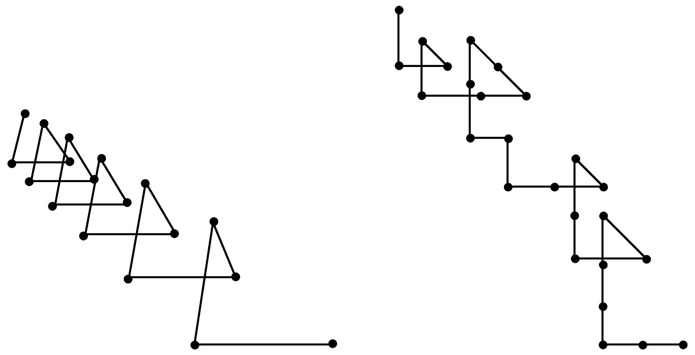
The monotone paths introduced and discussed in the previous sections can be regarded as irregular discrete helices. Figure 2 gives examples of two monotone paths in ${\mathbb{Z}}_{+}^3$. The one on the left resembles a discrete analog of a standard cylindrical helix, which is known as a triangular helix or regular skew-apeirogon. The one on the right features a similar (although irregular) helical structure, which we call an irregular discrete helix. Clearly, in dimensions higher than three, relevant illustrations are not possible. In dimension four, one can obtain certain evidence by viewing the projections of the monotone path on the four coordinate planes.

3.5. Negentropy of a Monotone Path

Broadly speaking, the term “negentropy” (short form of “negative entropy”) is interpreted as a trend towards creation, maintenance, and increasing order within a system. For this, “free energy” is utilized (which, according to the theory of thermodynamics, is energy available to perform work). In biology, negentropy hints at the capability of living organisms to create, maintain, and increase their internal order and complexity by utilizing free energy from the environment through metabolism and adaptation (thereby resisting the second law of thermodynamics).

For the purpose of adding the probabilities of independent events, the entropy is customarily defined as a logarithmic function. Likewise, we can define the negentropy of a monotone path L as

$$\mathcal{N}\left(L\right)={log}_2(1+mdv\left(L\right)),$$

or, alternatively, as 

$$\mathcal{N}\left(L\right)={log}_2(1+adv\left(L\right)).$$

We have $\mathcal{N}\left(L\right)\ge 0$, as $\mathcal{N}\left(L\right)=0$ if and only if L is an inline path.

In turn, the negentropy of a string s is

$$\mathcal{N}\left(L\left(s\right)\right)={log}_2(1+mdv\left(L\left(s\right)\right)(\mathrm{resp}. \mathcal{N}\left(L\left(s\right)\right)={log}_2(1+adv\left(L\left(s\right)\right)).$$

Let $\mathcal{S}$ be a set of strings and $\mathcal{L}\left(S\right)$ be the corresponding set of monotone paths. Then, the total negentropy of $\mathcal{L}\left(S\right)$ is

$$\mathcal{N}\left(\mathcal{L}\left(S\right)\right)=\sum _{s\in S}{log}_{2}mdv\left(L\left(s\right)\right)(\mathrm{resp}. \mathcal{N}\left(\mathcal{L}\left(S\right)\right)=\sum _{s\in S}{log}_{2}adv\left(L\left(s\right)\right)).$$

Note that the logarithmic function is strictly monotone; therefore, both $\mathcal{N}\left(L\right)$ and $mdv\left(L\right)$ (as well as $adv\left(L\right)$) are fairly good for comparative analysis of strings. Thus, as an alternative, one can measure the negentropy of a monotone path L according to its maximum (or average) deviation from linearity. As in the definition using a logarithmic function, $mdv\left(L\right)=0$ (resp. $adv\left(L\right)=0$) if and only if L is an inline path.

3.6. Monotone Graphs

Let $\mathcal{L}$ be a set of monotone paths in ${\mathbb{Z}}^n$, $n\ge 2$, and let $G\left(\mathcal{L}\right)$ be their union. $G\left(\mathcal{L}\right)$ can be regarded as a geometric graph, called monotone graph with vertices–the nodes of the paths, and edges–the grid edges of the paths in $\mathcal{L}$.

The monotone paths of $\mathcal{L}$ are subgraphs of $G\left(\mathcal{L}\right)$. If we assign directions on the edges of a path $L\in \mathcal{L}$, starting from the origin, we obtain a directed path $\overrightarrow{L}$ with the first vertex at the origin. Taking the directed paths $\overrightarrow{L}$ for all $L\in \mathcal{L}$, we obtain a directed graph $\overrightarrow{G}\left(\mathcal{L}\right)$.

• Properties of  $\mathit{G}\left(\mathcal{L}\right)$  and  $\overrightarrow{\mathit{G}}\left(\mathcal{L}\right)$

Property 1.

$G\left(\mathcal{L}\right)$ is connected. $\overrightarrow{G}\left(\mathcal{L}\right)$ is connected but not strongly connected and has no directed cycles.

Property 2.

In $G\left(\mathcal{L}\right)$ and $\overrightarrow{G}\left(\mathcal{L}\right)$, all simple monotone paths between any two vertices have the same length.

Property 3.

$G\left(\mathcal{L}\right)$ and $\overrightarrow{G}\left(\mathcal{L}\right)$ are rectilinear. According to Property 2, all cycles of $G\left(\mathcal{L}\right)$ are of even length. Hence, $G\left(\mathcal{L}\right)$ is bipartite (and, thus, 2-chromatic).

Property 4.

$G\left(\mathcal{L}\right)$ and $\overrightarrow{G}\left(\mathcal{L}\right)$ are sparse. (The proof is given in Appendix A).

Property 5.

$G\left(\mathcal{L}\right)$ is triangle-free (follows from Property 3).

Note: It is known [39] that a triangle-free graph $G(V,E)$ with sufficiently many edges (e.g., of the order of $\mathsf{\Omega }\left(n^2\right)$) is bipartite; otherwise, it may be non-bipartite. Monotone graphs are always bipartite, regardless their low density.

Property 6.

Both in $G\left(\mathcal{L}\right)$ and $\overrightarrow{G}\left(\mathcal{L}\right)$, one can find a shortest path from the origin to any vertex v in $O\left(p\right)$ time, where p is the length of the shortest path (searching backward from v to the origin). Clearly, all of them have the same length.

Property 7.

Since any subgraph of a bipartite graph is bipartite, for any vertex v in $G\left(\mathcal{L}\right)$, the subgraph reachable from v within $\overrightarrow{G}\left(\mathcal{L}\right)$ is a monotone graph.

4. Graph of Life

Graph-based methods are central in evolutionary biology for the study of interactions among proteins, genes, and DNA sequences (e.g., [40]). Previous monographs [41,42,43,44] provide a broad conceptual and methodological foundation for the use of graph theory in the biosciences. They collectively introduce the mathematical and computational principles underlying biological network analysis, ranging from metabolic and regulatory systems [42] to evolutionary and ecological interactions [44]. Foundational overviews of cellular organization through network structure [41] and general network theory with strong biological applications [43] further situate graph-based methods as central tools in modern biological research. A substantial body of research papers—too extensive to report in full here—has been developed on the subject, elucidating various facets of biological research. For instance, refs. [45,46,47,48] illustrate how graph-theoretic approaches have shaped contemporary systems biology. Scale-free network models [45] and centrality-based analyses of essential genes [46] demonstrate how structural properties of graphs reveal functional and evolutionary constraints. Methods for detecting overlapping communities [47] and for predicting protein function through network propagation [48] show how graph algorithms can extract biologically meaningful patterns from large-scale interaction data. Graph-based and graph grammar approaches to the modeling of structural determination, development, and evolution are investigated in [49].

Perhaps most widely used in the modeling of biological structures are bipartite graphs. For example, refs.  [50,51,52] highlight the particular relevance of bipartite graphs for the representation of heterogeneous biological relationships. Bipartite protein-complex networks [51] reveal modularity and organizational principles of the proteome, while bipartite gene-function mappings [50] support functional annotation and evolutionary inference. Bipartite transcription-factor target graphs [52] provide insight into regulatory architecture and its evolutionary constraints. Bipartite species-interaction networks [53] demonstrate how ecological and evolutionary structure emerges from mutualistic relationships, illustrating the versatility of bipartite models across biological scales. For applications of bipartite graphs in evolution and gene flow, as well as recent work on best-match graphs in phylogenetics, the reader is referred to [54].

In what follows, we define a graph in four-dimensional Euclidean space, which can be viewed as a geometric map of the biosphere’s viability region in nucleotide composition space.

DNA molecules consist of the adenine (A), guanine (G), cytosine (C), and thymine (T) nucleotide bases and can be represented as strings over the alphabet $\mathsf{\Sigma }=\{A,G,C,T\}$. Through string geometrization (Section 3.2), each sequence yields a monotone path $L\left(s\right)\in {\mathbb{Z}}_{+}^4$ whose coordinates correspond to the four bases. Every point of $L\left(s\right)$ represents a nucleotide position and defines a state in a state space embedded in ${\mathbb{Z}}_{+}^4$.

We define Graph of Life as $\mathcal{GL}=\bigcup L\left(s\right)$, the union taken over all living organisms. Similar networks can be formed for any biological group. $\mathcal{GL}$ is a monotone graph satisfying properties 1–7 and is extraordinarily large. With an estimated 8.7 million species and genomes ranging from millions to billions of bases, its size is of the order of ${10}^{12}$ to ${10}^{15}$. Individual variation further enlarges the network: about 20 quintillion animals existed in 2020, on Earth contains roughly $5\times {10}^{37}$ DNA base pairs, giving the scale of $\mathcal{GL}$’s nodes.

Beyond its size, $\mathcal{GL}$ is only partially known and constantly changing. Most species that have ever lived—over 99%—are extinct; new organisms appear and disappear, and mutations continually alter existing sequences. However, the network’s graph-theoretic properties remain stable. Conceptually, $\mathcal{GL}$ occupies a five-dimensional hyperspace, with time as the fifth dimension. Although not physically present in 3D space, it models all living organisms from their emergence approximately 4.1 billion years ago until the eventual end of life on Earth.

Note that the same construction applies verbatim to RNA-based organisms: their genomes also define monotone cumulative-count paths and an analogous graph representation with the same graph-theoretic properties as the DNA-based Graph of Life. Geometric descriptors $mdv$, $adv$, and $nlm$ can likewise be computed for RNA genomes, although their biological interpretation may differ because RNA organisms exhibit distinct compositional biases and evolutionary constraints.

4.1. Evolutionary Interpretation of the Graph of Life

The “Graph of Life” can be viewed as a compressed portrayal of genomic diversity. If every genome contributes a monotone path in $Z_{+}^4$, then the union of all these paths forms a gigantic geometric object encoding the global structure of genomic variation. This object is sparse (Property 4), which means that genomes occupy only a micro fraction of the theoretically possible space. In biological terms, this reflects strong restrictions: only a tiny subset of all possible DNA sequences is compatible with life. Sparsity is a mathematical way of demonstrating the idea that life traverses a thin, structured region of the entire sequence space.

Concurrently, the Graph of Life is bipartite (Property 3). Biologically, this suggests that the transitions between genomic states (as represented by monotone paths) feature a sort of hierarchical or directional constraint. This seems to be harmonious with evolution: genomes do not roam arbitrarily. Instead, they follow constrained trajectories shaped by selection, mutation biases, and biochemical feasibility.

The computational inferences of this construction are consequential. Sparse and bipartite graphs admit efficient algorithms for various problems that are NP-hard to solve on general graphs. Examples of such tasks are clustering (e.g., detecting groups of species), computation of distances between genomes (e.g., evolutionary divergence), ancestral reconstruction, and detection of structural “bottlenecks” of a biological system. These properties of the Graph of Life imply that wide-ranging comparative genomics may be more tractable than the underlying combinatorial complexity of the sequence space would suggest. In this sense, the graph provides not only a descriptive framework but also a computationally advantageous representation of genomic relationships. One could also suppose that the evolution may be navigating a space of DNA sequences whose structure makes adaptation feasible rather than combinatorially impossible.

Note also that in a dense, unconstrained sequence space, almost all random mutations would most probably be catastrophic. However, in a sparse and structured (bipartite) Graph of Life, neighboring genomes would tend to remain viable, with evolution proceeding through a network made of “safe” paths; as a result, catastrophic gamboling would naturally be avoided because they would lie outside the sparse region of DNA sequences. In other words, the geometry of the Graph of Life may reflect the fact that life evolves in a region of sequence space where survival is statistically stable.

Conceptually, the Graph of Life can be viewed as a geometric map of the biosphere’s viability region in sequence space. Its structure reflects the existence of “safe corridors” through which genomes can evolve while maintaining functionality. This perspective aligns with the broader view that evolution operates within a constrained environment shaped by biochemical feasibility and selective pressures. Thus, the graph offers a compact and informative representation of the deep structural constraints that govern genomic evolution, providing a foundation for future work on the geometry of sequence space, the dynamics of evolutionary change, and the global organization of genomic diversity.

The Graph of Life could be seen as a global viability manifold, which is a low-dimensional and structured subset of the astronomically large space of all DNA and RNA sequences where life can actually exist. The “good properties” of the graph can be viewed as a mathematical reflection of the fact that life has evolved within a constrained, navigable region of sequence space. Thus, life is possible because the underlying genomic space has a structure that the Graph of Life captures: sparse, constrained, and algorithmically passable rather than chaotic. See Figure 3 for a conceptual illustration.

4.2. Helical and Non-Helical Structures and Analysis Using Projections

DNA is not structurally uniform. The familiar Watson–Crick B-DNA double helix is the dominant form, but modern research has shown that DNA can adopt many alternative, experimentally confirmed structures under physiological conditions depending on the sequence, stress, and environment. These “non-canonical” forms are not rare curiosities. They appear in real genomes and often play regulatory or structural roles. Some alternatives remain helical (A-DNA, Z-DNA, and some triplexes), but many are not helices at all. For example, A-DNA is a compressed, right-handed helix often found in DNA–RNA hybrids. Z-DNA is a left-handed helix forming in GC-rich, torsionally stressed regions. G-quadruplexes are four-stranded stacks of planar G-tetrads—geometrically columns, not helices. i-Motifs are interlocked C-rich folds with no helical axis. Hairpins, cruciforms, and slipped structures form loops, branches, and misaligned segments rather than spirals. These structures appear in specific genomic contexts, such as telomeres, promoters, repetitive regions, and replication origins. Evolution preserves these non-helical shapes because they serve functional roles: regulating transcription, relieving torsional stress, protecting chromosome ends, controlling replication, shaping 3D genome architecture, and generating adaptive variation. They act as molecular switches, stress absorbers, binding platforms, and structural organizers. For more details, see [55,56].

For all the above alternative possibilities, the 4D monotonic path encodes sequence composition, not physical molecular geometry, i.e., it provides a mathematical encoding of the sequence, not a physical model of the molecule. The real 3D structure of DNA depends on various factors, such as electrostatic interactions, the hydration shell, ionic environment, protein binding, supercoiling, torsional stress, chromatin packing, temperature, pH, and mechanical forces inside the cell. These are not contained in the sequence alone, and none of them is represented in a monotonic 4D walk.

Note, however, that the 3D projections of the 4D monotone path on the four 3D coordinate planes can reveal informational geometry that correlates with structural and functional DNA behavior, including biologically meaningful features that are in tune with structure, function, and genomic behavior. Such features include the order of local nucleotide composition, long-range patterns, mirror-like local symmetry signals, and palindromes, which can form hairpins or cruciforms, periodicities, biases (GC-rich vs. AT-rich), motifs, and repeats. For example, strong drift in one coordinate highlights compositional bias (e.g., G-rich, implying potential G-quadruplex regions). Straight or nearly straight segments indicate tandem repeats or microsatellites, often linked to slipped-strand structures. Sharp bends or slope changes mark transitions between GC-rich and AT-rich domains, often aligning with regulatory boundaries. Dense, compact clusters in mixed C/G steps correspond to CpG islands and promoter regions. Periodic oscillations reflect structured repeats with known instability profiles. Large-scale curvature patterns can reflect isochores or replication domains. Thus, while projections cannot show the physical 3D shape of DNA, they reveal the sequence-encoded architecture that influences real DNA folding, stability, and function.

Projection from a 4D monotonic path into 3D inevitably removes one coordinate, but this loss does not undermine the biological conclusions one could draw from the geometry. The structural signals we care about, such as G-richness, palindromes, repeats, and domain boundaries, are encoded in patterns of cumulative drift rather than in the exact four-dimensional point. These patterns are geometric and remain visible, even when one axis is dropped. Features such as steep slopes, mirrored segments, straight lines, sharp bends, and compact clusters survive projection because they depend on relative changes among the remaining coordinates. Different projections can be used to recover different aspects of the sequence, much like viewing an object from multiple angles. The lost coordinate rarely contains unique structural information, since many biologically meaningful patterns arise from correlations among bases rather than from a single base count. The method is not intended to reconstruct the sequence but to detect large-scale compositional and structural tendencies. Because these tendencies produce strong geometric signatures, the conclusions remain reliable despite the dimensional reduction.

The 3D projections of a 4D monotonic path do not add new biological information, but they reorganize the sequence into a geometric form where important patterns become far easier to detect. Many meaningful features in DNA, such as G-rich stretches, palindromes, repeats, and GC/AT domain shifts, are present in the raw sequence but are visually subtle, scattered, or overlapping. When the sequence is converted into cumulative geometric drift, these same features produce strong shapes like steep slopes, mirror-symmetric curves, straight or periodic segments, sharp directional bends, or compact clusters. This transformation suppresses local noise and highlights long-range structure that is nearly impossible to see by reading the letters alone. It also allows different sequences with a similar functional architecture to produce similar geometric signatures, making comparisons intuitive. Palindromes and inverted repeats become literal reflections, and compositional transitions appear as abrupt changes in trajectory. Therefore, the projections serve as a kind of visual microscope for sequence architecture, revealing structural tendencies that remain hidden in symbolic form.

5. Negentropy of Species and Groups of Species

Most theories of the origin of life—RNA World, Oparin-Haldane [57,58], Metabolism First, and related scenarios—begin with some form of “primordial soup” from which the first organic molecules emerged. In this shared framework, simple inorganic compounds (water vapor and carbon-, hydrogen-, and nitrogen-containing species such as ammonia or methane) reacted to form the earliest organic monomers. Among these were canonical nucleobases adenine, guanine, cytosine, thymine, and uracil, which later assembled into RNA and DNA.

At this initial stage, these molecules did not exhibit any organized arrangement. They were not yet connected into macromolecules but existed as disordered collections of monomers, with no structural constraints and no long-range correlations. Their spatial and compositional distribution was effectively random. In this sense, on the eve of life’s emergence, organic matter existed as chaotic, unstructured aggregates of nucleobases. Such a state can be modeled, at the level of sequence statistics, by a random string of nucleotides. Its entropy is therefore maximal (and its negentropy minimal) compared with the structured genomes of later living organisms.

It is worth noting that low entropy alone does not imply biological relevance. A perfectly ordered system, such as a crystal at absolute zero, has zero entropy, but such a configuration is incompatible with life. In the language of sequence entropy introduced earlier, this would correspond to a string over a single-letter alphabet whose monotone path is perfectly linear and exhibits no deviation. Life requires structure but not perfect order. Chemical reactions in the prebiotic environment generally increase the entropy of the surrounding inorganic matter. However, these same processes can decrease the entropy (i.e., increase the negentropy) of the organic subsystem by producing more complex, more structured molecules. This reflects a fundamental thermodynamic trade-off:

An increase in the entropy of some inorganic matter was exchanged for a decrease in the entropy (increase in the negentropy) of certain organic matter.

This trade-off enabled the emergence of increasingly organized molecular structures, ultimately setting the stage for the appearance of life.

The definitions of Section 3.5 apply directly to the negentropy of DNA sequences and assemblies of such sequences. The negentropy of a DNA sequence s is

$$\mathcal{N}\left(L\left(s\right)\right)={log}_2(1+mdv\left(L\left(s\right)\right))(alternately, \mathcal{N}\left(L\left(s\right)\right)={log}_2(1+adv\left(L\left(s\right)\right))),$$

where $L\left(s\right)$ is the monotone path corresponding to s. Given a set $\mathcal{S}$ of a DNA sequences (in particular, S may be the entire Graph of Life $\mathcal{GL}$) and the corresponding set $\mathcal{L}\left(S\right)$ of monotone paths, the total negentropy of $\mathcal{L}\left(S\right)$ is

$$\mathcal{N}\left(\mathcal{L}\left(S\right)\right)=\sum _{s\in S}{log}_{2}mdv\left(L\left(s\right)\right)(alternately, \mathcal{N}\left(L\left(s\right)\right)=\sum _{s\in S}{log}_{2}mdv\left(L\left(s\right)\right)).$$

Let us reiterate that because of the monotonicity of the logarithmic function, both $\mathcal{N}\left(L\right(s\left)\right)$ and $mdv\left(L\right(s\left)\right)$ (resp. $adv\left(L\right(s\left)\right)$ can be used for any comparative studies concerning DNA sequences of species.

6. Experimental Study of DNA Sequences Grounded in Deviation from Linearity

The concept of string linearity provides a straightforward and practical method for comparing the DNA sequences of different organisms. It is natural to hypothesize that organisms with greater biological complexity possess more structured DNA whose associated monotone path deviates significantly from a straight line. In contrast, simpler organisms likely have less structured DNA, producing monotone paths that remain closer to linear. A fully random sequence over the alphabet {A,T,C,G} contains no inherent structure, so its monotone path should lie even nearer to a straight line.

To examine this hypothesis, experiments were conducted in two stages: first on an initial baseline panel of 25 species plus a random sequence, then on an expanded set of 50 species after adding 25 additional genomes and a random sequence. Reporting both stages allows us to show that the observed patterns are not artifacts of a small dataset but persist and even sharpen when the taxonomic breadth is doubled. This presentation highlights that the emerging geometric trends are robust, reproducible, and stable under substantial expansion of phylogenetic diversity.

In Stage 1 (25 species; see

Table A1. Normalized averages of 1000 trials.

Scientific Name	Common Name	Substrings			Subsequences
		adv	mdv	nlm	adv	mdv	nlm
Random Sequence	Random	12.8	12.8	100.0	9.4	8.9	100.0
H. Sapiens	Human	88.9	89.9	14.0	84.2	87.8	7.9
H. Neanderthalensis	Neanderthal	85.5	85.1	14.8	100.0	100.0	7.7
G. Gorilla	Gorilla	100.0	100.0	16.5	61.8	69.4	4.6
P. Troglodytes	Chimp	81.2	81.0	15.8	40.5	39.3	11.8
C. Familiaris	Dog	71.8	74.3	18.7	37.2	33.8	17.4
G. Gallus	Chicken	59.1	57.2	22.5	92.8	73.5	4.5
C. Jacchus	Marmoset	55.0	55.8	24.7	14.3	13.7	56.3
R. Norvegicus	Rat	68.2	68.0	22.9	31.6	30.5	13.9
M. Musculus	Mouse	62.5	64.9	19.8	15.5	14.9	49.7
O. Anatinus	Platypus	41.2	41.7	27.1	45.4	35.0	5.4
A. Carolinensis	Lizard	31.6	32.3	39.8	11.7	11.0	67.1
D. Rerio	Zebrafish	59.6	58.5	25.6	32.9	30.1	11.1
O. Latipes	Medaka fish	46.6	47.5	34.7	31.9	29.3	10.9
D. Melanogaster	Fruit fly	49.1	49.3	31.1	17.1	16.1	36.3
C. Intestinalis	Sea squirt	32.8	32.2	32.0	11.2	10.6	74.7
C. Elegans	Nematode	51.6	52.4	22.7	18.5	19.8	26.3
S. Cerevisiae	Yeast	39.4	39.8	27.4	12.7	11.7	74.1
C. Muridarum	Chlamydia	29.7	29.3	27.9	72.3	64.9	4.5
M. Tuberculosis	Tuberculosis	33.8	34.0	23.2	9.7	9.3	96.2
P. Gingivalis	Gingivalis	50.0	48.1	18.5	18.7	16.9	31.9
S. Thermophilus	Streptococcus	37.2	36.5	22.6	47.8	43.1	4.5
O. Sativa	Rice	73.8	76.9	24.5	14.9	14.0	63.5
Z. Mays	Corn	76.1	80.3	18.9	18.5	18.3	44.5
A. Thaliana	Cress	44.8	44.4	27.8	11.2	10.8	78.8
G. Max	Soybean	52.2	53.0	22.7	23.0	18.7	25.4
Maximum pre-normalized value:		554.5	1100.8	21.9	739.5	1563.6	22.4

), all DNA sequences were obtained from Ensembl Genomes, a genome-scale repository and browser maintained by the European Bioinformatics Institute, using the most recent assemblies available at the time the analyses were performed. The specific analyzed strains were: Chlamydia (Nigg), Tuberculosis (CCDC5180), Gingivalis (W83), and Streptococcus (ND03). All DNA samples were taken from chromosome 1 of each organism, with the exception of fruit fly and yeast, for which chromosomes 2L and 4 were used, respectively. For the additional 25 species included in Stage 2 (see

Table A3. Substring and subsequence statistics across species.

Group	Scientific Name	Common Name	Substrings			Subsequences
			adv	mdv	nlm	adv	mdv	nlm
Random Sequence			12.1	11.8	100.0	9.5	8.9	100.0
Primates	H. sapiens	human	85.9	82.6	13.6	84.2	87.8	7.6
	H. neanderthalensis	Neanderthal	84.8	82.5	14.0	100.0	100.0	7.5
	G. gorilla	gorilla	93.8	91.0	17.5	61.8	69.1	4.5
	P. troglodytes	chimpanzee	79.0	76.7	15.0	40.5	39.4	11.5
	Average		85.9	83.2	15.0	71.6	74.1	7.8
Mammals	T. truncatus	bottlenose dolphin	100.0	100.0	16.0	27.7	40.3	6.6
	B. musculus	blue whale	88.2	85.6	15.3	25.3	24.5	26.0
	C. familiaris	dog	66.6	66.9	19.0	37.5	33.9	17.1
	R. norvegicus	brown rat	65.1	63.0	21.7	31.7	30.6	13.7
	M. musculus	house mouse	61.0	62.6	18.5	15.6	14.9	48.9
	C. jacchus	common marmoset	52.6	52.4	24.0	14.3	13.8	55.0
	L. africana	African elephant	41.2	40.6	26.3	25.9	25.2	15.4
	O. anatinus	platypus	40.3	39.9	26.9	45.5	34.9	5.4
	Average		64.4	63.9	21.0	27.9	27.3	23.5
Other vertebrates	G. gallus	chicken	56.8	52.9	21.4	92.6	73.3	4.4
	C. moneduloides	New Caledonian crow	60.3	56.3	22.8	38.0	32.8	22.8
	P. major	great tit	52.7	51.5	28.7	17.8	20.7	23.2
	T. guttata	zebra finch	50.7	48.9	29.3	25.3	23.9	17.3
	M. ater	brown-headed cowbird	45.1	44.2	30.1	23.9	21.1	18.4
	A. carolinensis	green anole	30.3	30.3	37.7	11.6	10.9	66.9
	G. morhua	Atlantic cod	68.7	66.1	18.7	13.0	12.2	67.5
	D. rerio	zebrafish	55.6	52.6	25.2	32.4	29.7	11.4
	O. latipes	medaka	43.9	44.0	33.3	31.6	29.1	10.6
	Average		51.6	49.6	27.5	31.8	28.2	26.9
Invertebrates	A. californica	California sea hare	52.9	50.6	24.1	15.5	14.2	48.6
	C. elegans	nematode	49.5	49.0	22.4	18.4	19.8	25.7
	D. pulex	water flea	48.8	46.7	23.0	15.1	15.0	43.6
	B. mori	silkworm	44.7	47.0	28.2	19.2	16.3	34.4
	D. melanogaster	fruit fly	45.9	45.4	30.1	17.1	16.0	36.0
	T. adhaerens	placozoan	33.4	32.5	24.6	9.4	9.2	98.3
	C. intestinalis	sea squirt	31.2	29.7	31.0	11.1	10.7	71.9
	Average		43.8	43.0	26.2	15.1	14.5	51.2
Plants	Z. mays	corn/maize	71.1	73.2	19.1	18.6	18.4	43.0
	O. sativa	rice	69.3	69.9	24.1	14.8	14.0	62.6
	P. trichocarpa	black cottonwood	52.9	52.2	20.5	13.1	12.2	65.3
	G. max	soybean	50.6	49.9	22.1	23.0	18.7	24.7
	B. distachyon	purple false brome	50.6	49.8	28.9	12.0	11.1	86.5
	A. thaliana	thale cress	43.6	42.1	25.9	11.4	11.0	76.8
	Average		56.4	56.2	23.4	15.5	14.2	59.8
Fungi	N. crassa	red bread mold	62.3	61.3	33.3	18.5	19.0	34.8
	S. cerevisiae	yeast	37.2	36.5	26.7	12.6	11.6	73.1
	S. pombe	fission yeast	33.2	34.2	30.3	10.3	9.8	86.1
	Average		44.2	44.0	30.1	13.8	13.5	64.7
Protists	D. discoideum	slime mold	59.7	60.6	29.0	15.5	13.1	53.7
	C. reinhardtii	green alga	52.7	51.2	24.1	13.1	13.6	52.3
	L. major	leishmania parasite	52.0	48.1	25.5	15.8	14.8	38.5
	G. lamblia	giardia	45.7	44.4	16.8	13.0	12.8	62.8
	Average		52.5	51.1	23.9	14.4	13.6	51.8
Bacteria	P. gingivalis	oral bacterium	48.2	45.2	17.3	18.7	16.8	31.9
	S. coelicolor	soil actinomycete	40.7	39.8	19.2	19.6	17.8	24.3
	D. radiodurans	radiation-resistant bacterium	36.8	35.9	21.2	15.2	13.1	43.8
	P. fluorescens	fluorescent pseudomonad	35.4	34.8	22.3	25.7	23.8	8.1
	V. cholerae	cholera bacterium	36.0	34.0	22.6	23.2	23.3	11.2
	S. thermophilus	thermophilic streptococcus	34.4	33.0	23.4	47.7	43.0	4.4
	N. punctiforme	cyanobacterium	34.0	33.1	26.5	10.1	9.6	91.9
	M. tuberculosis	tuberculosis bacterium	33.6	32.6	22.0	9.8	9.3	94.5
	C. muridarum	mouse chlamydia	28.6	27.6	26.9	72.0	64.6	4.4
	Average		36.4	35.1	22.4	26.9	24.6	34.9

), sequences were obtained from a range of publicly available repositories (including Ensembl and other FASTA sources), selecting the most clearly annotated chromosomal or scaffold sequence available for each species. Together, these 50 genomes provide a representative and sufficiently diverse set for assessing the geometric properties of cumulative paths across species.

For each organism, we extracted relatively short substrings and subsequences in FASTA format, chosen at random from a genomic excerpt of approximately two million characters. We assumed that excerpts of this size are sufficiently large to mitigate the effects of genomic non-stationarity, though future work may involve sampling from complete genomes.

Our first step was to analyze how string length influences the proposed linearity measures and to determine an appropriate length for more extensive experiments. The results presented in the next section show that comparing samples of a reasonably chosen size yields the same relative ordering of organisms as comparisons based on much larger samples. Fixing the sample length also simplifies comparisons, since the absolute deviation from linearity depends on string length. Because genomes vary widely in size—and some remain incomplete or only partially studied—direct comparisons of full genomes are not feasible.

We also distinguish between substrings and subsequences of a string s: substrings consist of consecutive characters, whereas subsequences are ordered selections of characters that need not be consecutive. Most experimental work on biosequences focuses on substrings, but Apostolico and Cunial have recently explored the structure and randomness of polypeptides using subsequences satisfying specific constraints [29,30]. Their promising results motivated us to conduct all experiments using both substrings and subsequences. The similarities and differences between these two approaches are examined in the following sections.

6.1. Effects of Substring and Subsequence Length

Before detailing our research procedure, we explain our choice of data. We investigated how the length of a DNA sequence affects deviation from linearity and ascertained that deviation increases with the size of the string. However, the rate of increase appears independent of the organism, meaning that an organism’s deviation from linearity relative to others remains stable as long as all samples have the same sufficiently large length. Initial fluctuations disappear around lengths of approximately 50,000 bases, after which $mdv$ and $adv$ grow smoothly and predictably. For this reason, all subsequent analyses use substrings with a length of 50,000, which is long enough to suppress small-scale noise while remaining applicable to species with incomplete or unevenly assembled genomes. Using entire genomes would introduce confounding effects due to large differences in genome size and completeness, and focusing on specific genomic regions would shift the analysis toward local functional or structural features. Because our goal is to compare species as a whole, we average $mdv$ and $adv$ over 1000 uniformly chosen substrings per species, providing a stable estimate of each organism’s global compositional geometry rather than region-specific effects (e.g., taking care of regions that span centromeres, telomeres, microsatelites and other low-complexity regions) that would belong to other types of studies.

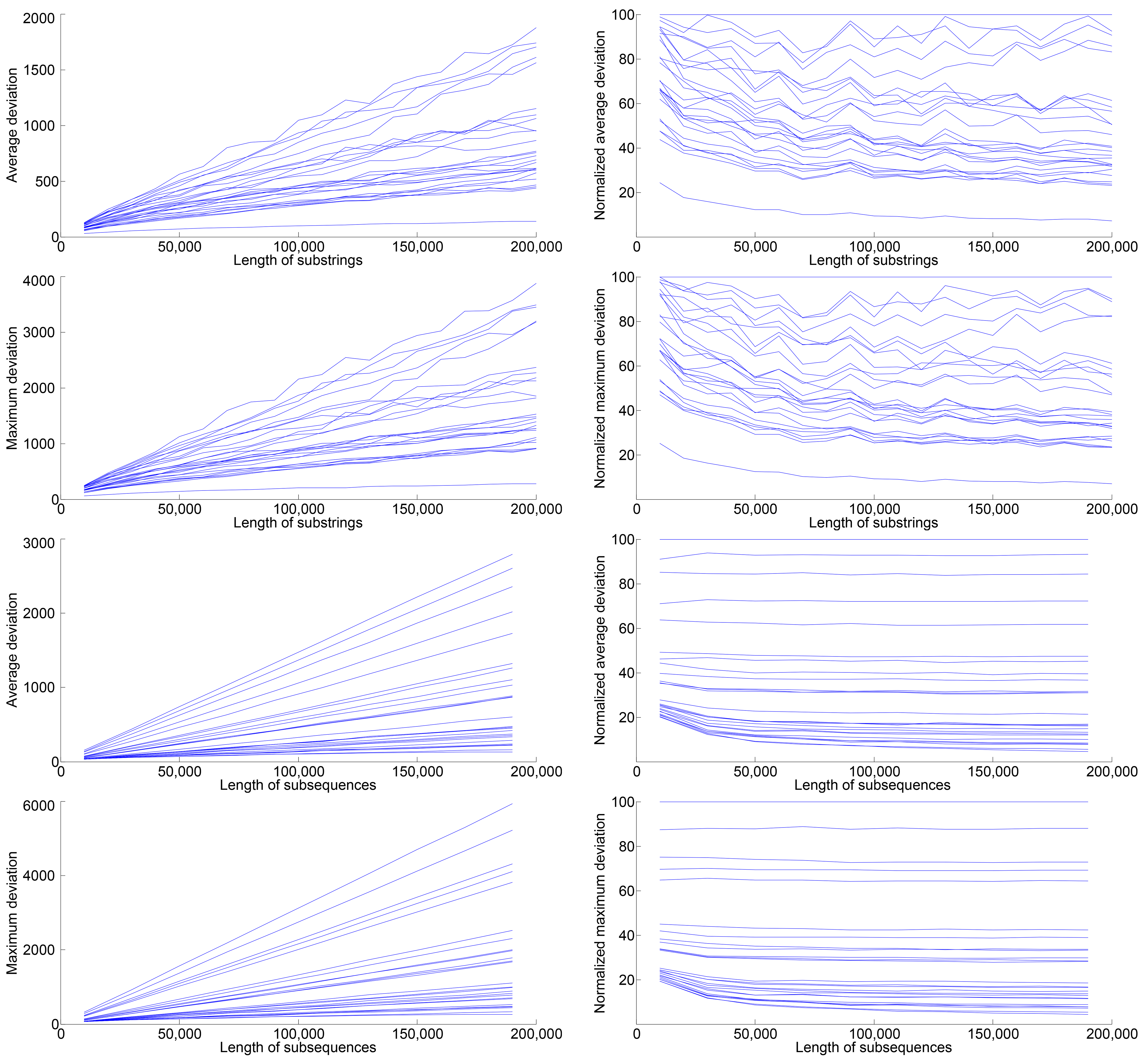
Figure 4 supports this observation by showing the absolute and normalized maximum and average deviations from linearity for substrings and subsequences of increasing length for our controlled baseline set of 25 species used in Stage 1. The top four graphs display the $adv$ and $mdv$ values for substrings, while the bottom four show the same measures for subsequences. The left column presents absolute values, and the right column shows the corresponding normalized values. The normalized graphs essentially “lift” the left sides of the absolute-value graphs, making the curves more directly comparable.

All substrings and subsequences were selected randomly from the 26 sources listed in Table A1. For the substring graphs, linearity measures were computed for lengths of $10,000\times k$ for $1\le k\le 20$. For each length, 200 random substrings were drawn from each source, and the average of these trials was plotted. For the subsequence graphs, lengths were $10,000\times (2k-1)$ for $1\le k\le 10$, with 100 randomly chosen subsequences per source; the averages of these trials were plotted. (Fewer lengths and trials were used for subsequences because additional resolution would not provide meaningful new information, given the near-linearity of the resulting graphs).

Figure 4 shows that $adv$ and $mdv$ derived from subsequences depend even less on length than those derived from substrings, as indicated by the reduced crossing of lines in the lower graphs. Nonetheless, even for substrings, the measures remain largely length-independent: across all tested lengths, organisms maintain roughly the same relative ordering.

As substring and subsequence lengths approach zero, deviation from linearity naturally approaches zero as well, and the measures become less stable. The normalized graphs indicate that initial fluctuations disappear around lengths of 50,000. For this reason, all subsequent experiments (which involve more trials) use substrings and subsequences with lengths of 50,000.

6.2. Description of Computational Procedure

The computations were performed using MATLAB R2011a for Stage 1 and MATLAB R2025b for Stage 2. We used the built-in randi and randseq functions to generate random selections and random sequences with independent, uniformly distributed symbols. We also used the peakfinder function from [35] to identify local extrema. The computational workflow consisted of three main components:

• Selection of samples;
• Computation of linearity measures;
• Compilation and normalization of data.

6.2.1. Selection of Samples

In both stages, to extract a random substring $b_1,\dots ,b_m$ from a larger string $a_1\dots a_n$, we selected a random integer $i\in [1,n-m_{+}1]$ using randi and set $b_j=a_i+j-1$ for $1leqj\le m$. Substrings of length m from each organism were stored in an array, along with a random sequence of length m over {A,T,C,G} generated using randseq. To obtain a random subsequence $b_1,\dots ,b_m$, we generated a list $C=c_1\dots c_m$ of m distinct random integers between 1 and n, sorted them to obtain $c_1<\cdots <c_m$, and set $b_i=a·c_i$ for $1\le i\le m$. These subsequences were stored in an array alongside a random sequence of the same length.

Because earlier analysis showed that fluctuations in linearity measures stabilize at a length of 50,000, all substrings and subsequences used in later experiments were chosen to have this length.

Because our geometric statistics are computed on long substrings (50 kb) and averaged over 1000 randomly sampled segments per species, they are expected to be robust to minor differences between successive assembly versions or small local corrections in updated releases. The focus of this work is on large-scale geometric organization of genomes rather than on fine-grained annotation; therefore, the precise assembly version is not expected to materially affect the qualitative patterns reported here. Using updated assemblies with explicit accession numbers would further enhance reproducibility, but this falls outside the scope of the present study.

6.2.2. Computation of Linearity Measures

For a string S of length m, we first count the occurrences $x_l$ of each letter $l\in \{A,T,C,G\}$, so that $\sum x_l=m$. Let $S_t$ denote the prefix of S of length t, and let $t_l$ be the number of occurrences of letter l in $S_t$, with $\sum t_l=t$. For each $1\le t\le m$, we compute the distance $D\left(S_t\right)$ from the point $(t_A,t_T,t_C,t_G)$ to the line through the origin and $(x_A,x_T,x_C,x_G)$ with the following formula:

$$\begin{array}{c}\hfill D\left(S_t\right)=\sqrt{{(x_{A}k-t_A)}^2+{(x_{T}k-t_T)}^2+{(x_{C}k-t_C)}^2+{(x_{G}k-t_G)}^2}\\ \hfill \mathrm{where}k={\displaystyle \frac{x_A{t}_A+x_T{t}_T+x_C{t}_C+x_G{t}_G}{x_A^2+x_T^2+x_C^2+x_G^2}}.\end{array}$$

The $D\left(S_t\right)$ values are stored in a list, from which we compute the average and maximum deviations, as well as the number of local maxima, using peakfinder.

6.2.3. Compilation and Normalization of Data

The two stages follow the same procedure. In Stage 1, for each set of 26 samples (25 biological sequences and one random sequence), we computed the linearity measures $adv$, $mdv$, and $nlm$, producing a $26\times 3$ table. This entire process was repeated 1000 times with different random samples. We then calculated the mean and standard deviation for each measure across the 1000 trials and normalized the mean values to highlight relationships among organisms. We also computed two measures of statistical dispersion: the coefficient of variation (CV), defined as the standard deviation divided by the mean, and the quartile coefficient of variation (QCV), defined as $(Q3-Q1)/(Q3+Q1)$, where $Q1$ and $Q3$ are the first and third quartiles. This procedure yields a table of normalized means that enables straightforward comparison of organisms across the three linearity criteria, along with a table summarizing variability across trials. The entire analysis was performed twice—once using substrings and once using subsequences. The results appear in Table A1 and

Table A2. Coefficient of variation (CV) and quartile coefficient of variation (QCV) of the 1000 trials.

Common Name	Substrings						Subsequences
	CV			QCV			CV			QCV
	adv	mdv	nlm	adv	mdv	nlm	adv	mdv	nlm	adv	mdv	nlm
Random	0.24	0.21	0.45	0.16	0.14	0.27	0.25	0.22	0.49	0.17	0.15	0.30
Human	0.43	0.42	0.71	0.29	0.28	0.33	0.05	0.03	0.25	0.03	0.02	0.33
Neanderthal	0.43	0.42	0.72	0.26	0.27	0.33	0.04	0.03	0.28	0.03	0.02	0.33
Gorilla	0.52	0.48	0.86	0.35	0.34	0.67	0.06	0.05	0.17	0.04	0.03	0.00
Chimp	0.43	0.43	0.78	0.27	0.28	0.33	0.10	0.06	0.27	0.06	0.04	0.20
Dog	0.43	0.41	0.60	0.28	0.26	0.50	0.07	0.08	0.20	0.05	0.06	0.14
Chicken	0.48	0.46	0.97	0.37	0.36	0.50	0.05	0.04	0.03	0.03	0.03	0.00
Marmoset	0.44	0.42	0.61	0.26	0.24	0.40	0.20	0.19	0.46	0.14	0.14	0.28
Rat	0.59	0.61	0.76	0.41	0.39	0.56	0.13	0.11	0.29	0.08	0.07	0.00
Mouse	0.33	0.36	0.57	0.23	0.26	0.25	0.22	0.20	0.49	0.15	0.13	0.33
Platypus	0.42	0.38	0.58	0.24	0.23	0.45	0.09	0.10	0.38	0.06	0.07	0.00
Lizard	0.33	0.32	0.51	0.23	0.22	0.38	0.19	0.18	0.44	0.13	0.12	0.29
Zebrafish	0.41	0.36	0.57	0.28	0.26	0.40	0.12	0.10	0.48	0.08	0.07	0.20
Medaka fish	0.42	0.37	0.54	0.26	0.25	0.43	0.12	0.11	0.38	0.09	0.08	0.20
Fruit fly	0.48	0.46	0.69	0.35	0.32	0.50	0.13	0.14	0.33	0.09	0.09	0.25
Sea squirt	0.34	0.31	0.59	0.21	0.20	0.38	0.25	0.23	0.47	0.16	0.16	0.31
Nematode	0.36	0.35	0.55	0.26	0.21	0.33	0.19	0.17	0.46	0.13	0.12	0.33
Yeast	0.33	0.30	0.40	0.18	0.20	0.27	0.25	0.22	0.46	0.17	0.15	0.27
Chlamydia	0.34	0.28	0.49	0.23	0.20	0.33	0.05	0.05	0.00	0.03	0.03	0.00
Tuberculosis	0.42	0.41	0.71	0.25	0.26	0.40	0.23	0.20	0.40	0.15	0.13	0.27
Gingivalis	0.46	0.45	0.58	0.30	0.28	0.43	0.19	0.18	0.48	0.13	0.12	0.29
Streptococcus	0.37	0.34	0.54	0.22	0.22	0.40	0.08	0.07	0.03	0.06	0.05	0.00
Rice	0.47	0.45	0.54	0.30	0.29	0.40	0.21	0.19	0.32	0.14	0.13	0.21
Corn	0.45	0.45	0.56	0.31	0.35	0.50	0.16	0.16	0.30	0.10	0.10	0.16
Cress	0.29	0.29	0.49	0.20	0.18	0.27	0.22	0.21	0.42	0.15	0.14	0.27
Soybean	0.34	0.33	0.48	0.19	0.21	0.33	0.14	0.13	0.41	0.10	0.09	0.27

.

Stage 2 repeats the same procedure on an expanded set of 50 species and a random sequence. The results appear in Table A3 and

Table A4. Coefficient of variation (CV) and quartile coefficient of variation (QCV) for substrings and subsequences.

Group	Scientific Name	Common Name	Substring						Subsequence
			CV			QCV			CV			QCV
			adv	mdv	nlm	adv	mdv	nlm	adv	mdv	nlm	adv	mdv	nlm
Random Sequence			0.26	0.23	0.48	0.18	0.16	0.33	0.25	0.22	0.47	0.17	0.15	0.32
Primates	H. sapiens	human	0.43	0.42	0.69	0.28	0.28	0.33	0.05	0.03	0.26	0.03	0.02	0.33
	H. neanderthalensis	Neanderthal	0.42	0.41	0.75	0.27	0.27	0.33	0.04	0.03	0.27	0.03	0.02	0.33
	G. gorilla	gorilla	0.53	0.50	0.85	0.35	0.36	0.43	0.06	0.05	0.17	0.04	0.03	0.00
	P. troglodytes	chimpanzee	0.41	0.42	0.79	0.27	0.27	0.33	0.09	0.05	0.25	0.06	0.04	0.20
Mammals	T. truncatus	bottlenose dolphin	0.88	0.90	0.74	0.38	0.29	0.33	0.13	0.08	0.53	0.09	0.05	0.33
	B. musculus	blue whale	0.54	0.51	0.62	0.38	0.38	0.43	0.12	0.09	0.23	0.09	0.06	0.17
	C. familiaris	dog	0.42	0.41	0.57	0.26	0.25	0.50	0.08	0.08	0.20	0.05	0.06	0.14
	R. norvegicus	brown rat	0.54	0.56	0.75	0.37	0.36	0.50	0.12	0.11	0.30	0.08	0.07	0.33
	M. musculus	house mouse	0.35	0.39	0.64	0.24	0.28	0.43	0.20	0.19	0.47	0.14	0.13	0.33
	C. jacchus	common marmoset	0.42	0.40	0.57	0.22	0.22	0.40	0.21	0.19	0.42	0.14	0.13	0.28
	L. africana	African elephant	0.34	0.34	0.55	0.23	0.22	0.27	0.14	0.13	0.33	0.10	0.09	0.14
	O. anatinus	platypus	0.43	0.41	0.59	0.26	0.24	0.45	0.10	0.09	0.39	0.06	0.06	0.00
Other vertebrates	G. gallus	chicken	0.48	0.46	0.97	0.35	0.36	0.50	0.04	0.04	0.00	0.03	0.03	0.00
	C. moneduloides	New Caledonian crow	0.65	0.60	0.86	0.43	0.41	0.56	0.09	0.08	0.14	0.06	0.05	0.09
	P. major	great tit	0.64	0.67	0.73	0.40	0.37	0.50	0.12	0.13	0.33	0.07	0.09	0.20
	T. guttata	zebra finch	0.65	0.64	0.65	0.34	0.35	0.50	0.12	0.12	0.37	0.08	0.09	0.25
	M. ater	brown-headed cowbird	0.47	0.46	0.68	0.31	0.31	0.50	0.09	0.10	0.31	0.06	0.07	0.25
	A. carolinensis	green anole	0.35	0.33	0.53	0.24	0.21	0.38	0.19	0.18	0.42	0.13	0.12	0.24
	G. morhua	Atlantic cod	0.66	0.60	0.66	0.24	0.25	0.43	0.19	0.16	0.35	0.13	0.11	0.24
	D. rerio	zebrafish	0.41	0.36	0.54	0.28	0.24	0.40	0.12	0.11	0.48	0.09	0.07	0.20
	O. latipes	medaka	0.41	0.38	0.54	0.26	0.26	0.43	0.13	0.11	0.39	0.09	0.07	0.20
Invertebrates	A. californica	California sea hare	0.40	0.38	0.67	0.27	0.27	0.43	0.23	0.22	0.45	0.17	0.15	0.27
	C. elegans	nematode	0.36	0.34	0.55	0.24	0.21	0.33	0.18	0.15	0.44	0.13	0.10	0.27
	D. pulex	water flea	0.42	0.41	0.77	0.29	0.28	0.33	0.20	0.20	0.39	0.14	0.13	0.26
	B. mori	silkworm	0.49	0.46	0.59	0.29	0.29	0.38	0.18	0.15	0.41	0.12	0.10	0.25
	D. melanogaster	fruit fly	0.49	0.47	0.68	0.36	0.33	0.50	0.13	0.14	0.33	0.09	0.09	0.25
	T. adhaerens	placozoan	0.33	0.32	0.54	0.22	0.21	0.40	0.25	0.23	0.46	0.18	0.15	0.29
	C. intestinalis	sea squirt	0.32	0.30	0.57	0.20	0.18	0.38	0.24	0.22	0.44	0.17	0.15	0.29
Plants	Z. mays	corn/maize	0.44	0.44	0.54	0.33	0.34	0.33	0.15	0.16	0.31	0.10	0.11	0.16
	O. sativa	rice	0.47	0.44	0.56	0.30	0.28	0.40	0.20	0.19	0.32	0.13	0.14	0.21
	P. trichocarpa	black cottonwood	0.30	0.28	0.49	0.21	0.20	0.33	0.20	0.18	0.39	0.13	0.12	0.24
	G. max	soybean	0.37	0.34	0.48	0.19	0.18	0.33	0.15	0.13	0.38	0.10	0.08	0.27
	B. distachyon	purple false brome	0.27	0.25	0.44	0.17	0.17	0.33	0.25	0.22	0.47	0.17	0.15	0.30
	A. thaliana	thale cress	0.28	0.27	0.45	0.17	0.17	0.27	0.23	0.21	0.42	0.15	0.14	0.29
Fungi	N. crassa	red bread mold	1.04	1.04	0.61	0.30	0.29	0.43	0.15	0.15	0.22	0.11	0.11	0.13
	S. cerevisiae	yeast	0.32	0.29	0.40	0.18	0.19	0.27	0.25	0.22	0.46	0.17	0.15	0.29
	S. pombe	fission yeast	0.36	0.35	0.45	0.20	0.21	0.29	0.26	0.24	0.47	0.18	0.16	0.30
Protists	D. discoideum	slime mold	0.38	0.35	0.56	0.26	0.24	0.33	0.22	0.19	0.33	0.15	0.11	0.22
	C. reinhardtii	green alga	0.36	0.34	0.51	0.21	0.20	0.40	0.21	0.18	0.38	0.14	0.12	0.22
	L. major	leishmania parasite	0.54	0.49	0.83	0.42	0.38	0.60	0.18	0.15	0.32	0.12	0.11	0.18
	G. lamblia	giardia	0.40	0.41	0.57	0.27	0.28	0.43	0.24	0.22	0.44	0.17	0.16	0.29
Bacteria	P. gingivalis	oral bacterium	0.47	0.45	0.57	0.28	0.26	0.43	0.18	0.17	0.47	0.12	0.11	0.29
	S. coelicolor	soil actinomycete	0.46	0.48	0.59	0.27	0.26	0.50	0.21	0.19	0.59	0.14	0.13	0.40
	D. radiodurans	radiation-resistant bacterium	0.46	0.46	0.55	0.22	0.22	0.33	0.21	0.17	0.40	0.14	0.11	0.26
	P. fluorescens	fluorescent pseudomonad	0.50	0.48	0.57	0.27	0.28	0.40	0.17	0.15	0.69	0.11	0.10	0.33
	V. cholerae	cholera bacterium	0.54	0.49	0.60	0.27	0.25	0.40	0.15	0.14	0.37	0.10	0.10	0.20
	S. thermophilus	thermophilic streptococcus	0.36	0.33	0.56	0.22	0.21	0.40	0.08	0.07	0.00	0.05	0.05	0.00
	N. punctiforme	cyanobacterium	0.33	0.31	0.49	0.22	0.19	0.27	0.23	0.21	0.44	0.16	0.14	0.30
	M. tuberculosis	tuberculosis bacterium	0.42	0.42	0.72	0.25	0.27	0.50	0.23	0.21	0.42	0.15	0.13	0.27
	C. muridarum	mouse chlamydia	0.32	0.28	0.47	0.22	0.20	0.33	0.05	0.05	0.00	0.04	0.04	0.00

.

7. Basic Results

This section expands on our experimental procedures and examines the results in greater depth. We highlight patterns that are readily apparent while acknowledging that additional insights may emerge for readers with more extensive expertise in the biological sciences.

7.1. General Observations and Comments

The first two columns of Table A1 (resp., Table A3) list the scientific and common names of the organisms included in our study. Columns 3–5 present the values of $adv$, $mdv$, and $nlm$ computed from substrings of the DNA sequences and one random sequence. The final three columns report the same measures computed from subsequences rather than substrings. Each measure was calculated on samples of length 50,000, averaged over 1000 trials.

• Stage 1. For most species, the normalized average values of $adv$ and $mdv$ derived from substrings differ by less than 1%. Only four organisms show differences greater than 2%, and none exceeds 4.2%. When subsequences are used, the discrepancy between $adv$ and $mdv$ is more variable: although typically under 2%, six organisms exceed 4%, and a few show differences as high as 10–20%. Table A2 further shows that the CV and QCV of $adv$ and $mdv$ differ by no more than 0.02 for most organisms and never by more than 0.06, regardless of whether substrings or subsequences are used. Figure 2 reinforces these similarities, as the $adv$ and $mdv$ curves are nearly indistinguishable, though slight differences appear more clearly in the subsequence-based plots.

Distributions with coefficients of variation below one are generally considered low-variance. As Table A2 indicates, the variance across the 1000 trials is, indeed, low, with subsequence-based trials showing substantially lower variance than substring-based trials.

We hypothesize that analyzing subsequences rather than substrings removes some structural information from the DNA, reducing precision. However, subsequences are less sensitive to sample length and exhibit lower variance. Substrings, by preserving the full local structure of the DNA, appear to yield linearity measures that more accurately reflect organismal complexity.

As shown in the fifth and eighth columns of Table A1, the $nlm$ measure effectively distinguishes random sequences from biological ones, but it is less informative for ranking organisms by biological complexity.

• Stage 2. Turning to Stage 2, we find that the expanded set of species exhibits qualitative patterns similar to those in Stage 1, thereby strengthening the overall conclusions.

The normalized differences between $adv$ and $mdv$ remain small for most organisms (at most, 4 and 1.47, on average), and subsequence-based values show somewhat larger discrepancies (at most 19.3 and 2.42 on average), just as in the smaller dataset. The corresponding CV and QCV values, again, indicate low variance across the 1000 trials. For substrings, the largest observed CV was 0.06 (with a mean of 0.02 across species), and the largest QCV was 0.09 (also averaging 0.02). Subsequences show consistently lower variability, with a maximum CV of 0.05 (mean of 0.02) and a maximum QCV of 0.04 (mean of 0.01). These findings reinforce the interpretation that subsequences, while less precise due to the loss of local structure, offer greater stability with respect to sampling length, whereas substrings preserve more of the geometric information relevant to organismal complexity.

As in Stage 1, $nlm$ effectively separates random sequences from biological ones but remains less informative for ordering species by complexity.

7.2. Distinction Between DNA Sequences and Random Sequences

Life is thought to have arisen from organic matter that initially existed as disordered collections of molecules characterized by chaotic, noisy, and highly variable chemistry—conditions that displayed a significant degree of randomness. From this environment, biological sequences gradually emerged through a complex evolutionary process whose precise mechanisms remain only partially understood.

A variety of earlier studies have used quantitative approaches to explore what, if anything, differentiates biological sequences from random ones, with mixed results. Although this objective has proven inherently difficult to pin down [59], considerable evidence suggests that biosequences exhibit many characteristics typically associated with randomness. One of the most striking is their extremely high—almost complete—incompressibility [60]. By many measures, biological sequences are barely distinguishable from their randomly permuted counterparts, even though such permutations are clearly incompatible with living systems [61,62,63]. While this observation may appear straightforward from a biological standpoint, numerous computational studies have also reinforced it. For instance, Pande et al. [64] mapped certain protein sequences onto Brownian bridges and observed subtle departures from pure randomness. Weiss et al. [65] estimated differential entropy and context-free grammar complexity, showing that large collections of non-homologous proteins are roughly 1% less complex than comparable sets of random strings. In the same study, the authors argue that DNA sequences can be viewed as “slightly edited random sequences” and that modern proteins may represent “memorized” ancestral random polypeptides that have been modestly refined by evolutionary pressures to enhance their stability under specific physiological conditions [29].

A key finding of our study is the clear separation between the linearity properties of biological and random sequences. Across all experiments, biological sequences exhibit higher average and maximum deviation from linearity than random sequences. This difference is especially pronounced when substrings are analyzed. In Table A1 referring to Stage 1, the normalized $adv$ and $mdv$ for the random sequence are both 12.8, whereas the smallest corresponding values among biological sequences are 29.3 and 29.7, respectively. Although the gap narrows when subsequences are used, random sequences still show the lowest deviation from linearity in every case. Figure 2 illustrates this distinction: in the substring-based plots (top row), the curve for the random sequence lies clearly below all others. In the subsequence-based plots (bottom row), the random sequence, again, forms the lowest curve, though the separation is less dramatic. The $nlm$ measure amplifies this contrast even further. For substrings, the normalized $nlm$ of the random sequence is 100.0, while the highest value among biological sequences is 39.8. For subsequences, the random sequence, again, attains 100.0, with the highest biological value being 96.2.

The results of Stage 2 (see Table A3) closely mirror those of Stage 1, confirming the robustness of the geometric trends identified above. More specifically, the normalized $adv$ and $mdv$ for the random sequence are 12.1 and 11.8, respectively, whereas the smallest corresponding values among biological sequences are 28.6 and 27.6, respectively. Although the gap narrows when subsequences are used, random sequences still show the lowest deviation from linearity. The only exception is the placozoan, whose subsequences yield $adv$ and $mdv$ values that approach—and, in the case of $adv$, slightly fall below—those of random subsequences. This behavior is expected because subsequences eliminate local genomic structure by sampling non-consecutive positions, thereby erasing motifs, repeats, and other contiguous patterns that normally increase deviation from linearity in biological DNA. Once this structure is removed, the descriptors depend primarily on global nucleotide composition. For organisms with relatively uniform and compositionally simple genomes, such as placozoans, subsequences can therefore produce geometric measures that are nearly indistinguishable from or marginally lower than those of fully random sequences.

The $nlm$ measure accentuates the separation between random and biological sequences. For substrings, the normalized $nlm$ of the random sequence is 100.0, whereas the highest biological value is 37.7. For subsequences, the random sequence, again, reaches 100.0, with the highest biological value at 98.3.

Given the approximately 1% difference reported in [65], our experiments revealed discrepancies of several hundred percent when comparing DNA sequences to random sequences constructed over the same alphabet and of identical length. This leads to the following conclusion:

DNA sequences exhibit substantially higher average and maximum deviation from linearity than random sequences.

These striking differences support the following assertion:

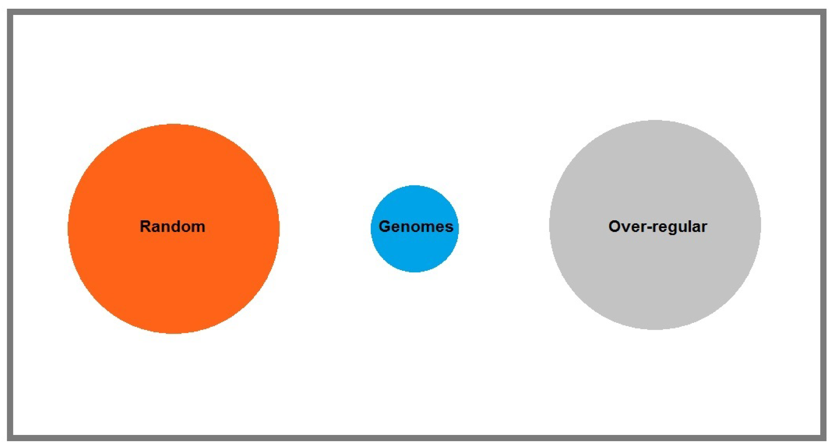
DNA sequences cannot be regarded as minor perturbations of random sequences. The degree of departure from randomness is substantial, even though many randomness-related properties—such as incompressibility—have been largely preserved.

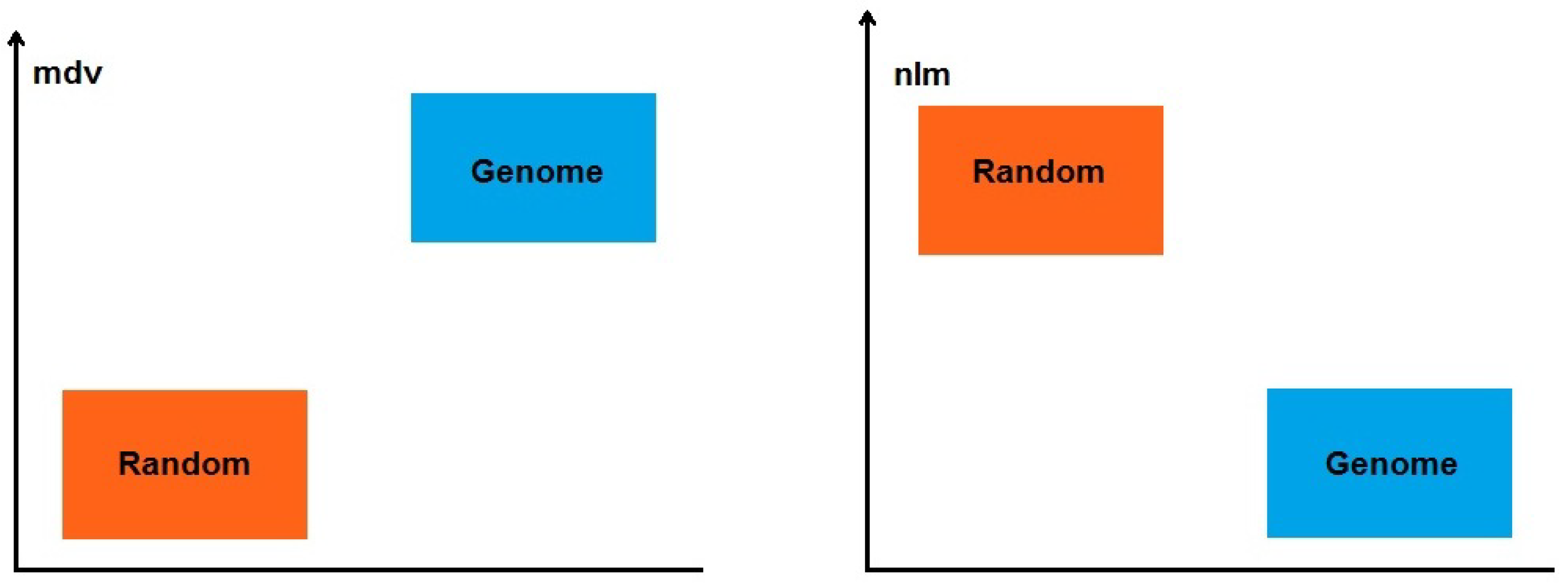
See Figure 5 for a conceptual illustration.

We conclude this section with one additional remark concerning the necessity of testing other random models.

Real DNA sequences cannot be captured by any single simple stochastic model. Rather than behaving like one homogeneous i.i.d. (i.i.d. stands for independent and identically distributed sequence of random variables), Markov, or Poisson process, genomes resemble mixtures of many short-range models whose parameters vary along the sequence. Different regions exhibit different base compositions, transition patterns, and local statistical structures, so the overall sequence is only “quasi-random” rather than stationary. Models like the ones listed above can each describe local behavior, but none can account for the full heterogeneity of genomes.

For random sequences with fixed letter probabilities, the monotone path $q_i,i=1,2,\dots ,m$, behaves like a random walk with drift. The segment $\overline{q_0{q}_m}$ is the drift line, and the deviations form a centered fluctuation process and are measured relative to the single global-drift line segment. According to classical limit theorems, these fluctuations scale as $\sqrt{m}$ and converge to a Gaussian bridge. Consequently, for a strng s of a length m both $mdv\left(s\right)$ and $adv\left(s\right)$ grow on the order of $\sqrt{m}$, with constants determined by the covariance of the underlying distribution. This $\sqrt{m}$ scaling holds for a broad class of short-range dependent models including those listed above because they all satisfy functional central-limit theorems. Therefore, it is not necessary to repeat our experiments for each of these models individually, since they all produce the same $\sqrt{m}$-scale deviations and yield results comparable to the uniform random case.

7.3. Rise of Deviation from Primitive to Biologically Complex Organisms

Given the widely accepted principles of evolutionary theory and the available theoretical and experimental evidence, it is reasonable to hypothesize that as organisms evolved from primitive forms to more biologically complex ones, their corresponding DNA sequences also evolved from sequences that were random or nearly random toward sequences exhibiting progressively greater deviation from randomness.

For the purposes of our analysis, we treated bacteria and microscopic organisms as the most primitive life forms. Plants were considered the next level of complexity, followed by fish, reptiles, and other egg-laying vertebrates. Mammals and primates were placed at the highest end of the evolutionary spectrum. We anticipated that the degree of deviation from linearity would increase in a manner consistent with this hierarchy of biological complexity. Our experiments, based on the measures introduced earlier, largely supported this expectation (though not with the same level of decisiveness observed when comparing random sequences to DNA sequences).

More specifically, in Stage 1, humans, neanderthals, gorillas, and chimpanzees exhibit the highest values of $adv$ and $mdv$. At the opposite end, bacterium Chlamydia shows the smallest $adv$ and $mdv$ after the random sequence. Other organisms with low deviation from linearity include tuberculosis, sea squirt, and lizard (Green anole). Organisms such as the fruit fly, medaka fish, and soybean fall into the mid–low range, while zebrafish, chicken, and mouse occupy the mid–high range (see Table A1 in Appendix B).

Another noteworthy observation is that primates tend to have lower $nlm$ (number of local maxima) values than other animals. Beyond this, however, the $nlm$ measure appears less effective than the other metrics for distinguishing organisms by biological complexity.

The analysis of Stage 2 produces patterns that remain consistent with those of Stage 1, aside from small variations attributable to the broader species set, thereby confirming the robustness of the geometric trends identified above. The highest $adv$ and $mdv$ values were observed in dolphin, whale, humans, neanderthals, gorillas, and chimpanzees, whereas Chlamydia, again, shows the smallest values after the random sequence. Other organisms with low deviation from linearity include fission yeast, as well as sea squirt and lizard. Primates, whale, and dolphin typically have lower $nlm$ values than other animals. Beyond this observation, this metric provides limited resolution compared with the other metrics.

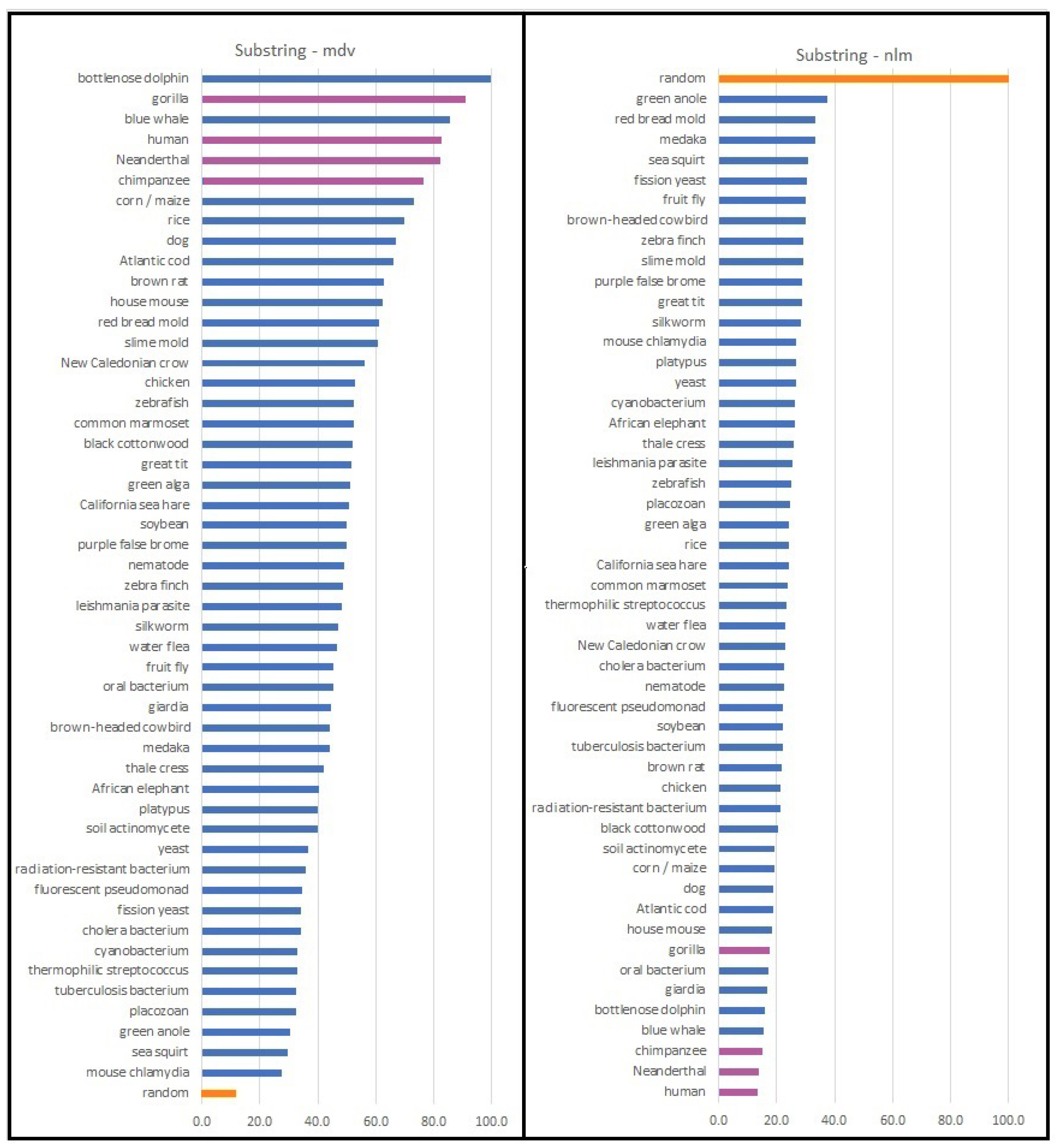
See Figure 6 for illustration. Species are ordered by their $mdv$ and $nlm$ values to make the distribution and outliers visually clear. This ordering is purely for readability and does not affect the underlying comparisons.

7.4. Evolutionary Interpretation of Multiscale Genomic Geometry

As predicted by stochastic models, random sequences exhibited the smallest $mdv$ and $adv$ values, consistent with the $\sqrt{m}$-scale fluctuations of a drifted random walk. In contrast, real genomes showed substantially larger deviations, with a general trend of rising $mdv$ and $adv$ from more primitive to more complex organisms, albeit with exceptions. These results indicate that genomes of complex organisms contain stronger long-range compositional heterogeneity and more coherent structural domains, producing large divergence away from the global-drift line in the cumulative-count geometry.

Complementing these global measures, the $nlm$ statistic captured local irregularity of the monotone paths. Here, the trend was reversed: primate genomes exhibited markedly fewer local maxima than those of the other examined species, indicating smoother local trajectories despite their large-scale deviations. This combination—high $mdv$/$adv$ but low $nlm$—suggests that complex genomes deviate strongly from linearity but do so through broad, smooth compositional arcs rather than through short, jagged fluctuations. In contrast, simpler organisms exhibit smaller global deviations but more fragmented local structure. Together, $mdv$, $adv$, and $nlm$ provide a multiscale geometric characterization of genomic organization, revealing systematic differences in both global and local structure across the evolutionary spectrum.

Within the Graph of Life framework, these findings integrate naturally. Each genome contributes a monotone path embedded in the shared four-dimensional viability region of sequence space. Species with low $mdv$/$adv$ and high $nlm$ values (e.g., bacteria) traverse short, locally irregular trajectories, while species with high $mdv$/$adv$ and low $nlm$ values (e.g., primates) follow long, smooth, heterogeneous arcs through the same constrained manifold. Thus, the three deviation measures enrich the interpretation of the Graph of Life by quantifying how different lineages navigate the global genomic landscape with distinct geometric signatures. While these patterns are consistent with stronger or more coordinated evolutionary constraints in complex organisms, they do not, by themselves, distinguish the relative contributions of mutational biases, selection, and genomic architecture. Instead, they provide a geometric framework within which such mechanisms can be investigated.

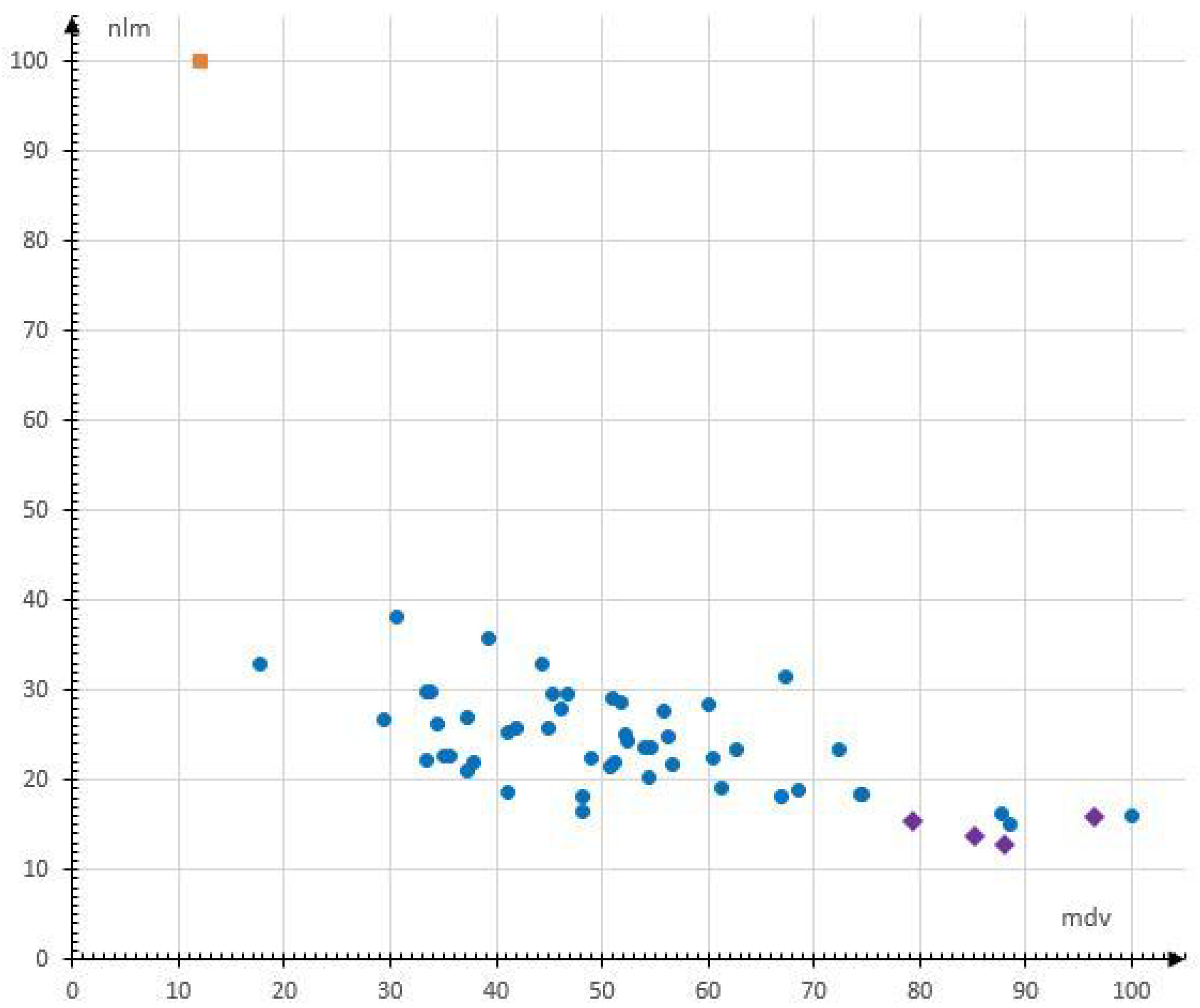
For illustration, see the scatterplot of $mdv$ versus $nlm$ for the 50 examined species and random sequences presented in Figure 7.

• Exceptions to the Trend and Their Genomic Basis

Although the overall pattern showed increasing $mdv$ and $adv$ from bacteria to primates, several notable deviations were observed, each reflecting lineage-specific genomic architecture rather than contradictions of the general trend.

A first class of exceptions arises from plant genomes: when measured over substrings, rice and corn show relatively high $mdv$ and $adv$ values—higher even than those of mouse and rat. This is consistent with the distinctive structure of many plant lineages. Cereals and other large plant genomes often contain extensive transposable element expansions, long blocks of repetitive sequence, and remnants of ancient whole-genome duplications, all of which create broad compositional domains and pronounced long-range excursions in the cumulative-count geometry. These features can inflate global deviation measures independently of organismal complexity.

A second class of exceptions emerged only after expanding the dataset to 50 species. Several mammals outside the primate clade—most notably, dolphin and whale—now occupy the extreme high-$mdv$/$adv$ end, surpassing gorilla, which was the top species in the smaller dataset. This shift is biologically consistent: cetaceans are known for unusually homogeneous, compositionally stable genomes. Group-level averages further illustrate these architectural influences: primates show the highest mean $mdv$ and $adv$, followed by other mammals, plants, protists, and other vertebrates, whereas invertebrates, fungi, and bacteria occupy progressively lower ranges. These differences reflect well-established genomic properties: mammals and many plants possess long, compositionally uniform domains; protists include lineages with large, smooth genomes, while invertebrates and bacteria typically exhibit more fragmented, heterogeneous sequence organization.

A third apparent exception was the elephant, which showed relatively low $mdv$ and $adv$ and a comparatively high $nlm$ values. This is consistent with the known architecture of elephant genomes, which are highly repeat-rich and compositionally heterogeneous; moreover, our sampling covered only a portion of the genome, likely capturing a structurally complex region. Thus, the elephant does not represent an anomaly but reflects genuine genomic heterogeneity within mammals.

Taken together, these exceptions highlight that $mdv$ and $adv$ capture a combination of evolutionary, architectural, and compositional influences, and they underscore the importance of interpreting geometric signatures within the broader context of each lineage’s genomic organization rather than as direct proxies for organismal complexity.

The evolution of different species is influenced by a variety of factors and ultimately represents a sequence of events, some of which occur by chance. This naturally leads to numerous exceptions to general evolutionary trends. At times, such anomalies serve as catalysts for new hypotheses and scientific debate.

7.5. DNA-Based Viruses

As noted earlier, our study focuses primarily on species from the Tree of Life, and viruses are therefore not a central object of analysis. Nevertheless, we conducted additional experiments on five DNA-based viruses whose genomes are sufficiently large to allow for application of our geometric framework. These viruses were evaluated alongside the other 50 species, enabling direct comparison. Results for the more informative substring-based analysis are presented in

Table A5. Substring statistics including a group of DNA-based viruses.

Group	Scientific Name	Common Name	adv	mdv	nlm
Random Sequence			12.9	12.6	100.0
Primates	H. sapiens	human	91.0	88.5	13.9
	H. neanderthalensis	Neanderthal	89.1	86.8	13.8
	G. gorilla	gorilla	100.0	97.0	16.7
	P. troglodytes	chimpanzee	84.0	81.1	15.9
	Average		91.0	88.4	15.1
Mammals	T. truncatus	bottlenose dolphin	99.9	100.0	16.4
	B. musculus	blue whale	95.6	93.4	15.3
	C. familiaris	dog	70.4	70.3	19.6
	R. norvegicus	brown rat	67.9	66.7	22.5
	M. musculus	house mouse	64.4	65.7	19.3
	C. jacchus	common marmoset	54.8	54.8	25.1
	L. africana	African elephant	43.1	43.0	26.5
	O. anatinus	platypus	42.9	42.3	26.7
	Average		67.4	67.0	21.4
Other vertebrates	G. gallus	chicken	61.0	57.2	21.1
	C. moneduloides	New Caledonian crow	63.7	59.1	23.1
	P. major	great tit	56.1	55.4	29.4
	T. guttata	zebra finch	55.3	53.3	29.1
	M. ater	brown-headed cowbird	48.0	46.8	29.7
	A. carolinensis	green anole	31.8	31.9	38.9
	G. morhua	Atlantic cod	73.0	70.9	18.4
	D. rerio	zebrafish	60.0	57.3	24.8
	O. latipes	medaka	46.9	46.9	33.8
	Average		55.1	53.2	27.6
Invertebrates	A. californica	California sea hare	56.9	54.5	24.0
	C. elegans	nematode	52.9	52.1	22.3
	D. pulex	water flea	50.3	48.4	24.1
	B. mori	silkworm	49.1	51.6	28.6
	D. melanogaster	fruit fly	49.2	48.4	30.9
	T. adhaerens	placozoan	35.0	34.3	24.7
	C. intestinalis	sea squirt	33.5	31.9	31.4
	Average		46.7	45.9	26.6
Plants	Z. mays	corn/maize	77.1	80.5	18.8
	O. sativa	rice	74.4	75.6	24.6
	P. trichocarpa	black cottonwood	56.3	55.1	20.9
	G. max	soybean	53.5	53.1	22.5
	B. distachyon	purple false brome	54.1	53.5	29.2
	A. thaliana	thale cress	46.4	45.2	26.9
	Average		60.3	60.5	23.8
Fungi	N. crassa	red bread mold	68.1	67.0	32.8
	S. cerevisiae	yeast	39.3	38.7	27.3
	S. pombe	fission yeast	34.4	36.1	31.9
	Average		47.3	47.3	30.7
Protists	D. discoideum	slime mold	64.6	65.3	28.6
	C. reinhardtii	green alga	59.1	57.4	23.4
	L. major	leishmania parasite	53.4	50.5	26.5
	G. lamblia	giardia	49.1	48.2	17.3
	Average		56.6	55.4	24.0
Bacteria	P. gingivalis	oral bacterium	50.3	47.5	18.5
	S. coelicolor	soil actinomycete	43.7	42.8	18.6
	D. radiodurans	radiation-resistant bacterium	39.4	38.5	22.2
	P. fluorescens	fluorescent pseudomonad	38.8	38.0	22.2
	V. cholerae	cholera bacterium	39.9	37.7	22.0
	S. thermophilus	thermophilic streptococcus	38.2	36.6	22.5
	N. punctiforme	cyanobacterium	36.5	35.9	26.6
	M. tuberculosis	tuberculosis bacterium	34.4	33.6	23.3
	C. muridarum	mouse chlamydia	30.7	29.6	27.4
	Average		39.1	37.8	22.6
DNA-Viruses	Acanthamoeba castellanii		45.4	45.7	21.1
	Acanthamoeba polyphaga		27.5	27.1	59.5
	Megavirus chiliensis		42.4	43.7	24.4
	Pandoravirus dulcis		29.9	29.8	60.6
	Pandoravirus salinus		27.4	26.8	59.9
	Average		34.5	34.6	45.1

, while

Table A6. Coefficient of variation (CV) and quartile coefficient of variation (QCV) for substrings including DNA-based viruses.

Group	Scientific Name	Common Name	CV			QCV
			adv	mdv	nlm	adv	mdv	nlm
Random			0.25	0.22	0.46	0.17	0.15	0.29
Primates	H. sapiens	human	0.42	0.42	0.75	0.27	0.26	0.33
	H. neanderthalensis	Neanderthal	0.41	0.41	0.70	0.26	0.27	0.33
	G. gorilla	gorilla	0.52	0.48	0.82	0.35	0.35	0.43
	P. troglodytes	chimpanzee	0.44	0.44	0.76	0.29	0.28	0.33
Mammals	T. truncatus	bottlenose dolphin	0.76	0.76	0.72	0.37	0.26	0.33
	B. musculus	blue whale	0.51	0.48	0.65	0.36	0.36	0.33
	C. familiaris	dog	0.42	0.42	0.58	0.26	0.25	0.50
	R. norvegicus	brown rat	0.54	0.57	0.79	0.37	0.38	0.56
	M. musculus	house mouse	0.34	0.37	0.59	0.25	0.27	0.43
	C. jacchus	common marmoset	0.42	0.40	0.59	0.23	0.23	0.40
	L. africana	African elephant	0.31	0.31	0.51	0.22	0.21	0.27
	O. anatinus	platypus	0.43	0.40	0.56	0.26	0.24	0.45
Other vertebrates	G. gallus	chicken	0.47	0.44	1.02	0.32	0.33	0.50
	C. moneduloides	New Caledonian crow	0.64	0.59	0.87	0.41	0.38	0.56
	P. major	great tit	0.66	0.70	0.74	0.42	0.40	0.50
	T. guttata	zebra finch	0.66	0.65	0.67	0.35	0.36	0.50
	M. ater	brown-headed cowbird	0.47	0.46	0.68	0.30	0.30	0.50
	A. carolinensis	green anole	0.33	0.31	0.53	0.23	0.21	0.38
	G. morhua	Atlantic cod	0.63	0.58	0.62	0.23	0.23	0.43
	D. rerio	zebrafish	0.39	0.35	0.54	0.28	0.25	0.40
	O. latipes	medaka	0.41	0.37	0.54	0.27	0.27	0.43
Invertebrates	A. californica	California sea hare	0.38	0.36	0.66	0.26	0.25	0.40
	C. elegans	nematode	0.35	0.33	0.53	0.24	0.19	0.33
	D. pulex	water flea	0.43	0.42	0.78	0.27	0.27	0.33
	B. mori	silkworm	0.54	0.50	0.63	0.31	0.31	0.50
	D. melanogaster	fruit fly	0.49	0.46	0.70	0.35	0.32	0.50
	T. adhaerens	placozoan	0.32	0.31	0.51	0.20	0.21	0.40
	C. intestinalis	sea squirt	0.34	0.31	0.55	0.20	0.20	0.38
Plants	Z. mays	corn/maize	0.42	0.44	0.54	0.31	0.34	0.50
	O. sativa	rice	0.47	0.44	0.56	0.31	0.29	0.40
	P. trichocarpa	black cottonwood	0.32	0.29	0.48	0.21	0.20	0.33
	G. max	soybean	0.36	0.34	0.46	0.19	0.19	0.33
	B. distachyon	purple false brome	0.27	0.24	0.44	0.19	0.17	0.33
	A. thaliana	thale cress	0.29	0.28	0.48	0.20	0.18	0.33
Fungi	N. crassa	red bread mold	1.04	1.04	0.59	0.30	0.28	0.43
	S. cerevisiae	yeast	0.30	0.28	0.39	0.17	0.18	0.27
	S. pombe	fission yeast	0.33	0.36	0.48	0.20	0.21	0.29
Protists	D. discoideum	slime mold	0.37	0.34	0.52	0.25	0.23	0.33
	C. reinhardtii	green alga	0.36	0.36	0.55	0.22	0.21	0.40
	L. major	leishmania parasite	0.55	0.50	0.83	0.40	0.36	0.60
	G. lamblia	giardia	0.42	0.42	0.60	0.28	0.30	0.43
Bacteria	P. gingivalis	oral bacterium	0.45	0.44	0.59	0.28	0.26	0.50
	S. coelicolor	soil actinomycete	0.45	0.45	0.60	0.26	0.27	0.43
	D. radiodurans	radiation-resistant bacterium	0.51	0.51	0.58	0.24	0.25	0.40
	P. fluorescens	fluorescent pseudomonad	0.52	0.51	0.58	0.27	0.27	0.40
	V. cholerae	cholera bacterium	0.56	0.52	0.64	0.27	0.26	0.33
	S. thermophilus	thermophilic streptococcus	0.39	0.36	0.56	0.23	0.21	0.33
	N. punctiforme	cyanobacterium	0.33	0.30	0.48	0.22	0.20	0.27
	M. tuberculosis	tuberculosis bacterium	0.41	0.41	0.68	0.25	0.27	0.40
	C. muridarum	mouse chlamydia	0.32	0.28	0.47	0.22	0.20	0.33
DNA-Viruses	Acanthamoeba castellanii		0.51	0.53	0.48	0.25	0.26	0.33
	Acanthamoeba polyphaga		0.40	0.37	0.44	0.21	0.20	0.31
	Megavirus chiliensis		0.57	0.58	0.51	0.25	0.26	0.27
	Pandoravirus dulcis		0.29	0.27	0.36	0.18	0.17	0.23
	Pandoravirus salinus		0.37	0.33	0.43	0.22	0.19	0.31

reports the corresponding CV and QCV values.

Three of the viruses (Acanthamoeba polyphaga, Pandoravirus dulcis, and Pandoravirus salinus) display the lowest $adv$ and $mdv$ values—comparable only to mouse chlamydia—and the substantially highest $nlm$ values, whereas the remaining two viruses (Acanthamoeba castellanii and Megavirus chiliensis) do not exhibit such extreme behavior. Overall, the average $mdv$ (34.62) and $adv$ (34.52) values across the five viruses are the lowest among all species groups, while their average $nlm$ (45.1) is, by far, the highest.

We also observed that in this experimental round, the gorilla, again, attains the highest $adv$ (100), followed closely by the dolphin (99.9), whereas the dolphin achieves the highest $mdv$ (100), followed by the gorilla (97.0).

7.6. Deviation of Biosequences Relative to Permutational Extremes

As mentioned previously, it is natural to ask how far a DNA sequence s departs from linearity relative to the greatest possible deviation among all permutations of its symbols (denoted $maxmdv\left(s\right)$). Given the patterns observed in the preceding sections, our goal is to determine whether DNA sequences could, through further evolution, develop even greater deviation from linearity or whether their current structures are already close to the theoretical maximum. Applying Theorem 1 to a four-letter alphabet (the case relevant for DNA) yields the following result.

Corollary 1.

For $n=4$, ${max}_{mdv}\left(L\left(s\right)\right)$ is the maximum of the terms:   

$\sqrt{{\displaystyle \frac{a_1^2(a_2^2+a_3^2+a_4^2)}{a_1^2+a_2^2+a_3^2+a_4^2}}}$, $\sqrt{{\displaystyle \frac{a_2^2(a_1^2+a_3^2+a_4^2)}{a_1^2+a_2^2+a_3^2+a_4^2}}}$, $\sqrt{{\displaystyle \frac{a_3^2(a_1^2+a_2^2+a_4^2)}{a_1^2+a_2^2+a_3^2+a_4^2}}}$, $\sqrt{{\displaystyle \frac{a_4^2(a_1^2+a_2^2+a_3^2)}{a_1^2+a_2^2+a_3^2+a_4^2}}}$,

$\sqrt{{\displaystyle \frac{(a_1^2+a_2^2)(a_3^2+a_4^2)}{a_1^2+a_2^2+a_3^2+a_4^2}}}$, $\sqrt{{\displaystyle \frac{(a_1^2+a_3^2)(a_2^2+a_4^2)}{a_1^2+a_2^2+a_3^2+a_4^2}}}$, and $\sqrt{{\displaystyle \frac{(a_1^2+a_4^2)(a_2^2+a_3^2)}{a_1^2+a_2^2+a_3^2+a_4^2}}}$.

If, for instance, the first of these seven quantities is the largest for the given values of $a_i$, then the strings whose discrete monotone paths pass through either $(a_1,0,0,0)$ or $(0,a_2,a_3,a_4)$ achieve $mdv\left(L\right(s\left)\right)$. Concretely, this includes all strings beginning with $x_1{a}_1$ and all strings ending with $x_1{a}_1$. Using this result, we computed the ratio of $maxmdv/mdv$ for DNA sequences from human, gorilla, mouse, zebrafish, and tuberculosis and for a random sequence, considering substrings of lengths $1,\dots ,10\times {10}^5$ (see

Table A7. The ${max}_{mdv}/mdv$ ratio computed for substrings of length $\{1,\dots ,10\}\times {10}^5$.

Human	17.3	15.0	12.6	13.2	15.6	10.5	13.1	11.4	14.3	12.2
Gorilla	12.7	20.1	15.2	12.0	11.8	13.5	13.0	11.2	10.6	10.9
Mouse	19.9	28.1	30.8	40.2	37.9	41.7	45.2	57.1	46.7	50.0
Zebrafish	28.2	24.9	27.7	32.7	31.7	28.6	32.8	37.0	26.6	40.8
Tuberculosis	44.6	64.8	66.5	84.6	88.1	96.5	105.1	116.3	122.5	144.9
Random Sequence	126.7	164.3	205.7	260.2	280.7	304.7	325.1	336.0	351.2	397.0

in Appendix B). Interpreting deviation from linearity as an indicator of structural organization, the data suggest the following:

All organisms retain substantial potential for further structural complexity.

As expected, the ratios vary across organisms, with more primitive species exhibiting larger values than more complex ones. The smallest observed ratio of $maxmdv/mdv=10.5$ occurs for a 600,000-base substring of the human genome. In contrast, the largest ratio among biological sequences, i.e., 144.9, is found in a 1,000,000-base substring of the tuberculosis genome. For comparison, a random 1,000,000-base substring reaches an even higher value of 397.

8. Hypotheses and Biological Interpretations Derived from the Results

It is worth noting that progress in the natural sciences has often relied on a productive interplay between speculative theorizing and empirical validation. Many foundational ideas, such as general relativity, antimatter, dark matter, and gravitational waves, were initially proposed on theoretical grounds long before direct evidence became available. Biology, too, has seen influential theories rise and fall as new data have emerged, reflecting the evolving nature of empirical understanding. In this broader context, speculative frameworks can play a constructive role by articulating conceptual possibilities, identifying new questions, and guiding the search for empirical signatures. The geometric perspective developed here is offered in this spirit: as a theoretical lens that may help illuminate aspects of genomic organization and, potentially, the deeper transitions that shaped the emergence of life.

Based on the empirical patterns observed across the diverse set of genomes analyzed here, several broader conjectures naturally emerge. These hypotheses are not presented as definitive biological laws but, rather, as informed proposals suggested by the geometric regularities uncovered in our study. They are intended to guide future theoretical development and empirical testing and to highlight potential directions in which the geometric perspective on genomic organization may have explanatory value.

8.1. Equilibrium Condition for Life

Life emerged and evolved under conditions in which chemical reactions and mutations were not directed but largely stochastic. Beneficial changes were retained because they improved survival or replication, yet the underlying mutational input remained fundamentally random. From this perspective, the gradual accumulation of structural organization in early nucleic acids can be viewed as a form of increasing negentropy—a departure from randomness that enabled more complex and adaptive biological functions.

At the same time, this process could not proceed without constraint. If genomic sequences became too regular or too compressible, they would lose the capacity to encode large amounts of information and would become overly predictable, reducing their functional potential. Modern genomes are strikingly incompressible, and this near-maximal incompressibility appears to be a prerequisite for storing and maintaining the vast informational content required for cellular life. In information-theoretic terms, systems with low entropy are more predictable and carry less information, whereas systems with higher entropy can encode richer and more diverse messages. Therefore, genomes cannot drift toward excessive regularity without compromising their informational capacity. This suggests that the evolution of life required a balance: increasing structural organization and functional complexity, on one hand, and the preservation of high informational capacity through incompressibility, on the other. In this view, biological systems occupy a regime where randomness and structure coexist in a productive equilibrium—enough order to support function and adaptation yet enough unpredictability to encode large amounts of information efficiently and without redundancy.

Conjecture 1.

Life is possible only when a sensible equilibrium is maintained between negentropy (structural organization) and incompressibility (informational capacity).

This conceptual perspective aligns with broader ideas in the literature that describe life as a process shaped by thermodynamic constraints (see, e.g.,  [66]) and by the need to maintain functional organization, securing higher complexity and adaptivity. It is offered here not as a definitive explanation but as a hypothesis motivated by the geometric and statistical properties observed in genomic sequences.

8.2. Local Maxima as a Geometric Descriptor

Recall that local maxima were identified using MATLAB’s peakfinder function, which detects peaks that stand out relative to their local neighborhoods. In this characterization, a higher $nlm$ corresponds to a more irregular or “jagged” cumulative path, whereas a lower $nlm$ indicates a smoother trajectory with fewer noticeable deviations from the global drift line determined by the endpoints of the path. It is known that random (or closer to random) sequences are geometrically “more jagged” than nonrandom sequences that would have more predictable structures. With a reference to our experimental results, as expected, the normalized average of $nlm$ on 1000 trials with random sequences equals 100 in both stages. In Stage 1, those for the primates, i.e., human, neanderthal, gorilla, and chimp, are 14.0, 14.8, 16.5, and 15.8, respectively. These values are substantially lower than all of the other species that we have tested (the average $nlm$ for all 25 examined species being 21.9). See Table A1 in Appendix B. Stage 2 (Table A3) shows a similar trend. The four primates have $nlm$ values of 13.6, 14.0, 17.5, and 15.0 (mean of 15.0), which are generally lower than those of the remaining species (overall mean of 24.4). Dolphin and whale exhibit similarly low values (16.0 and 15.3) comparable to those of the primates.

The above indicates that in the cumulative-count geometry, the primate genomes possess smoother large-scale compositional trajectories than the genomes of the other species that were analyzed. This pattern suggests the following:

Conjecture 2.

Primate genomes possess a comparatively more homogeneous or less fragmented compositional structure.

Various factors may contribute to this difference, such as the inclusion of lineage-specific mutational biases, constraints on the variation of GC content, the distribution of repetitive elements, or differences in genome architecture. One possible hypothesis is that the smoother monotone paths reflect stronger or more consistent evolutionary constraints acting on primate genomes. However, further analysis is needed in order to distinguish the relative contributions of mutational processes and natural selection. Presently, this observation could be interpreted as a sturdy geometric signature rather than as straight evidence for a specific evolutionary mechanism.

Taken together, these hypotheses highlight a unifying theme (extending the idea introduced in the previous section): genomic sequences appear to be shaped by a balance between structural organization and informational capacity, a balance that manifests geometrically in the cumulative-count representation. The smoothness of cumulative-count paths, the bounded range of deviation from linearity, and the apparent equilibrium between negentropy and incompressibility all suggest that genomes are neither maximally random nor maximally regular but, instead, reside in an intermediate regime that supports both functional complexity and high information density. All these point toward a constrained region of genomic configuration space that living systems occupy. These constraints do not arise from the geometric framework itself; rather, the framework makes them visible by translating sequence composition into measurable geometric traits.

Therefore, the conjectures proposed here serve two complementary purposes. First, they provide a conceptual interpretation of the empirical signatures uncovered by our geometric descriptors. Second, they outline a set of testable predictions about how genomes may be organized across species and through evolutionary time. Future work may refine these ideas by incorporating phylogenetic modeling, examining additional clades, or extending the geometric analysis to other biological polymers. For now, the hypotheses underscore the potential of geometric approaches to reveal broad organizing principles of genomic architecture.

8.3. Borders of Life

The results of Section 7.6 can be interpreted in another way. Consider the value of $100\times mdv/{max}_{mdv}$ (the percent of the reciprocal of ${max}_{mdv}/mdv$), which represents the percentage that the deviation of a species constitutes with respect to the possible maximum range of the species’ deviation. The maximum and minimum percentages are reached for the same species: 0.69% for tuberculosis and 9.5% for human, while for a random substring, the average ratio equals 0.32%. These values are obtained for sufficiently long substrings (6,000,000, resp. 1,000,000 nucleotide bases for the two species and 1,000,000 for the random sequence). This provides evidence that the degree of deviation of species is within certain bounds: a lower bound that is a fraction smaller than 1 (lower-bounded by the percentage for the random substring) and an upper bound (over all species) that seems to be not considerably greater than 10%. More precise bounds could be established through extensive experimentation, but the initial results indicate that these limits are unlikely to shift dramatically.

This raises a natural question: Can deviation from linearity increase indefinitely as evolution proceeds, or are there intrinsic limits? Our interpretation is that genomic deviation from linearity is constrained by two opposing requirements. A lower bound is imposed by the level of structural organization (negentropy) necessary to sustain biological complexity and functionality. A genome that is too close to randomness would lack the long-range structure required for coordinated regulation and organismal viability. Conversely, an upper bound is imposed by the need to maintain high incompressibility. As discussed earlier, excessive regularity would reduce informational capacity, increase predictability, and ultimately compromise the ability of the genome to encode diverse and finely tuned biological functions.

Conjecture 3.

These two constraints define a region of permissible genomic organization— “borders of life” measured in terms of deviation from linearity. Exceeding these borders in either direction would lead to gradual degradation and, eventually, to loss of viability.

This perspective is compatible with broader ideas in the literature that view life as a system maintained by thermodynamic flows and constrained by the need to balance order and unpredictability. In this sense, the deviation-from-linearity trait may reflect a deeper equilibrium between structural organization and informational capacity, a balance that appears necessary for the persistence of living systems.

9. Speculative Outlook: Geometric Irregularity, Transitional States, and the Emergence of Biological Complexity

A broader speculative perspective suggested by our findings is that the origins and subsequent evolution of life may be viewed through the geometry of self-replicating macromolecules. Early replicators in most origins-of-life scenarios are assumed to have been short, structurally simple, and close to linear chains, whereas increasing structural irregularity is associated with the emergence of catalytic pockets, binding specificity, and functional diversification. From this viewpoint, geometric deviation from linearity can be interpreted as a proxy for informational capacity and biochemical versatility, reflecting the transition from simple templated replication to molecules capable of folding, regulation, and interaction. Although highly conjectural, this geometric framing is compatible with established theoretical models in which viable sequences occupy a constrained, structured subset of sequence space and where evolutionary innovation corresponds to the exploration of increasingly irregular regions of that space. The idea does not claim direct empirical support but offers a unifying conceptual lens through which the geometric descriptors introduced here may be connected to deep questions about the emergence and expansion of biological complexity.

The geometric descriptors developed in this work naturally invite broader reflection on the transition from inanimate organic matter to the earliest living systems. While the emergence of new organisms today follows well-understood biological processes, the origin of the first autonomous replicators remains far less clear. Contemporary definitions of life typically require cellular organization, metabolism, replication, responsiveness, and adaptive capacity, yet is not obvious that these criteria must appear simultaneously or that the boundary between non-living and living matter is sharply defined.

One possibility is that early prebiotic systems passed through intermediate states—entities that possessed some but not all of the features associated with life. Such “protoliving” structures may have exhibited primitive forms of metabolism, compartmentalization, or information storage without yet achieving full biological autonomy. In this view, the transition from inanimate to animate matter would not be a discrete event but a gradual process unfolding over extended periods of chemical evolution.

A complementary perspective is that the emergence of life may be associated with surpassing a threshold of structural organization or negentropy. Within the geometric framework developed here, such organization could be reflected in quantitative measures such as deviation from linearity or average deviation. Although it is impossible to determine the precise numerical value that might correspond to such a threshold, the conceptual point is that a minimal degree of informational structure may be required before a system can sustain the functions typically associated with living matter.

These two perspectives are not mutually exclusive. A protoliving entity may have gradually accumulated structural organization until it crossed a threshold compatible with autonomous replication and adaptive evolution. While these ideas extend beyond the empirical scope of the present study, they illustrate how geometric and information-theoretic descriptors might contribute to future theoretical discussions about the origin of life. They are offered here as speculative remarks intended to stimulate further thought rather than to propose definitive mechanisms.

10. Concluding Remarks

This work has developed a geometric framework for analyzing biological sequences and has demonstrated that large-scale geometric descriptors—such as deviation from linearity, local irregularity, and path-based negentropy—capture fundamental structural properties of genomes across the Tree of Life. The presented results obtained here indicate that these measures are not merely mathematical curiosities but reflect genuine biological organization. The consistent patterns observed across diverse species suggest that geometric constraints may play a central role in shaping viable sequence space and in distinguishing biological sequences from random polymers.

The evidence accumulated in this study points toward a coherent picture: genomic sequences occupy a highly structured region of sequence space, and their geometric properties correlate with broad evolutionary and organizational features. The monotone path representation and the monotone Graph of Life, together, provide a unified mathematical substrate for comparing species, quantifying complexity, and exploring the boundaries of biological organization. These constructions offer a promising alternative to traditional combinatorial approaches and open the possibility of a genuinely geometric theory of genomic structure.

Beyond the specific results obtained here, the work introduces a broadly applicable geometric technique for genome analysis. By treating DNA sequences as monotone paths and monotone graphs and by defining associated quantitative descriptors, the framework provides a reusable methodological tool that can be applied to a wide range of comparative, evolutionary, and structural questions. This positions the approach not only as a conceptual contribution but also as a technique that other researchers can adopt, extend, and integrate into their own analyses.

Several directions for future research follow naturally from the present work. A priority is the development of rigorous metrics on monotone paths and monotone graphs, which would enable quantitative comparison of species and support clustering, phylogenetic reconstruction, and the study of evolutionary trajectories within the geometric framework. Equally important is the systematic application of these descriptors to large genomic datasets including hundreds or thousands of species to determine the extent to which the observed trends generalize and to identify lineage-specific signatures. A deeper biological interpretation of local maxima and minima of geometric deviation (potentially linked to functional domains, regulatory regions, or evolutionary hotspots) represents another promising avenue.

The conceptual implications are equally significant. The results suggest that increasing geometric irregularity may accompany—and perhaps enable—the transition from simple replicators to complex organisms. This raises the possibility that the emergence of life and the evolution of complexity can be viewed as trajectories within a geometric landscape constrained by the structure of viable sequence space. Such a perspective offers a unifying lens through which questions about the origin of life, evolutionary innovation, and the theoretical limits of biological complexity may be reconsidered.

The present work is primarily descriptive and methodological: it introduces and characterizes geometric measures of genomic organization across a broad phylogenetic range. Analyses relating these geometric descriptors to specific biological covariates, such as base composition, coding density, or effective population size, would address a different level of explanation and would require additional data, careful model specification, and explicit control for phylogenetic relatedness. Such investigations are scientifically interesting and may help illuminate potential evolutionary drivers of the observed geometric patterns, but they constitute a substantial extension of the current framework. We therefore view them as promising directions for future research rather than components of the present study, whose aim is to establish and explore the geometric properties themselves.

This study is intended as a foundation for a broader research program. The mathematical structures introduced here, together with the empirical patterns they reveal, provide a basis for a more comprehensive interdisciplinary effort involving mathematics, computational biology, molecular evolution, and origins-of-life research. The framework is flexible, extensible, and capable of supporting both theoretical development and large-scale empirical analysis. We believe that the geometric viewpoint advanced in this work has the potential to reshape how genomic organization is quantified and understood and to contribute meaningfully to the long-standing effort to uncover the principles that govern the emergence and evolution of living systems.