Fuzzy Iterative Learning Contouring Control

Abstract

Iterative learning contouring control (ILCC) improves contouring accuracy in multi-axis motion systems via the equivalent contour error formulation. However, its convergence strongly depends on the learning gain. Large gains may induce overly aggressive updates and local divergence, degrading performance, whereas small gains lead to slow convergence. Moreover, contour error convergence is typically non-uniform along the trajectory, and local divergence may still occur despite global convergence, particularly near error saturation regions. To address these issues, a fuzzy inference mechanism is integrated into the online ILCC framework, yielding an online ILCC with fuzzy-regulated convergence parameters (online ILCCf), enabling adaptive regulation of the learning gain. Two regulation strategies are developed: (i) online ILCCf_i, an independent multi-parameter regulation scheme; and (ii) online ILCCf_u, a unified single-parameter regulation scheme. The fuzzy mechanism adaptively adjusts the convergence parameters online according to the instantaneous magnitude of the equivalent contour error. Experimental results on a six-axis industrial robot demonstrate fast convergence while maintaining satisfactory contouring performance. Among all comparison cases, online ILCCf_i achieves the best performance, reducing the RMS position error from $7.26\times {10}^{-1}$ mm to $5.93\times {10}^{-2}$ mm and the RMS orientation error from $6.95\times {10}^{-4}$ rad to $5.64\times {10}^{-5}$ rad, without oscillation or local divergence. Further simulations confirm robustness under model uncertainty and measurement noise.

1. Introduction

In practical manufacturing environments, machining tasks are often repetitive, particularly in mass-production scenarios. This repetitive nature makes iterative learning control (ILC) an attractive solution, since control commands can be progressively refined from cycle to cycle by exploiting the error information obtained in previous executions. Compared with conventional feedback and feedforward schemes, ILC is effective in compensating for servo lag, repetitive disturbances, and model uncertainties [1,2]. Owing to these advantages, ILC has been extensively applied over the past decades to motion systems such as CNC machine tools [3,4], industrial robots [5,6], semiconductor manufacturing equipment [7,8], and various precision motion platforms.

ILC algorithms can be formulated either in the frequency domain [9,10,11] or in the time domain [5,12], and can be further categorized into model-free ILC [13,14] and model-based ILC [2,15]. Furthermore, from the perspective of control objectives, ILC can be classified into tracking control [2,6] and contouring control [16,17]. Tracking control aims to minimize the deviation between the actual position and the reference command, which is quantified by the tracking error [12,18]. In contrast, contouring control focuses on minimizing the deviation between the executed trajectory and the desired geometric path, which is quantified by the contour error [19,20]. Motivated by machining applications in five-axis machine tools and industrial robots, this study adopts a time-domain, command-based, model-based discrete ILC framework for contouring control. Specifically, the contour error obtained in the current iteration is utilized to iteratively update the control command for the subsequent iteration.

The contouring control task is more challenging than tracking control. It mainly involves two key components, namely contour error estimation [21] and contour error control [22]. However, most existing approaches rely on approximate contour error models, which may introduce modeling inaccuracies and consequently degrade contouring performance. Furthermore, for five-axis machine tools and industrial robots, contouring ILC becomes more difficult because both position contour error and orientation contour error must be addressed, owing to the involvement of orientation control as well as highly coupled and complex kinematics and dynamics in the motion task [13,14]. In addition, accurate estimation of position and orientation contour errors usually incurs a high computational burden, which limits the applicability of such methods in real-time industrial implementations [13,14].

Motivated by the limitations of conventional contouring methods, Chen et al. proposed an iterative learning contouring control (ILCC) framework [15], in which the equivalent contour error [19] is adopted as the control objective instead of the actual contour error model, and the method was originally validated on biaxial motion systems. It has been theoretically and experimentally demonstrated that reducing the equivalent contour error guarantees a reduction in the actual contour error [15]. An important advantage of the ILCC framework is that it can be naturally and conveniently extended to five-axis machine tools and industrial robots [23]. This is mainly because the equivalent contour error can be computed accurately and efficiently from the analytical description of the desired path, without relying on approximate geometric contour models. Moreover, ILCC performs learning directly in the machine coordinate system (MCS), rather than in the task coordinate system (TCS) [13,14], which would otherwise require repeated kinematic and dynamic transformations and may introduce additional numerical errors and computational burden.

Despite the effectiveness of ILCC [15,23] and the computational convenience of evaluating the equivalent contour error, the overall algorithm still involves nontrivial computations, including the construction of the learning gain matrix and the update of command inputs, which introduce noticeable computational and time burdens. Although the equivalent contour error can be computed efficiently in real time, existing ILCC implementations are predominantly based on offline (batch) learning, where parameter updates are performed only after the completion of an entire machining cycle. Consequently, the machine must be paused for learning updates before the next cycle, which is undesirable in practical production environments. Although more recent ILC-based contouring control methods [20,24] have been proposed, they still rely on optimization-based contour error estimation, which introduces significant computational overhead and limits real-time applicability. Moreover, the dependence on estimated contour error may degrade contouring performance due to estimation inaccuracies.

In practical manufacturing environments, machining operations are usually required to be executed in a continuous manner without interrupting the production process. However, studies on online learning strategies specifically targeting contouring control remain very limited. An online ILC scheme was reported in [25], in which a model-free learning structure was adopted to enable real-time implementation with low computational complexity. Nevertheless, model-free ILC generally lacks theoretical guarantees on monotonic convergence, and its learning objective is formulated for trajectory tracking rather than for contouring accuracy. An online learning compensation method based on model prediction was later proposed by Wang et al. [26]. This approach is also designed to reduce tracking errors and does not explicitly address contouring performance. To overcome these limitations, an online iterative learning contouring control (online ILCC) framework was recently developed in [27], in which the contouring objective is directly incorporated into the online learning process. The proposed framework enables real-time updating of learning commands for machining tasks in CNC machine tools and industrial robots, while explicitly targeting contour error reduction under continuous-operation conditions.

A significant limitation remains in ILC [2], ILCC [23], and online ILCC [27]: the design of the learning matrix, particularly the selection of the learning gain, plays a critical role in determining convergence behavior. If the learning gain is too large, the learning process becomes overly aggressive and may lead to divergence, thereby degrading contouring performance and producing large contour errors in certain trajectory segments. Conversely, if the learning gain is too small, the learning process becomes overly conservative, resulting in slow convergence and a large number of learning iterations. In industrial machining applications, where productivity is critical, an increased number of learning iterations directly translates into higher production costs. Therefore, appropriate tuning of the learning gain is a key issue in ILCC algorithms.

Moreover, contour error convergence is typically non-uniform along both the trajectory and learning iterations, and local divergence may still occur despite global convergence, particularly near error saturation regions. Accordingly, it is desirable to adapt the learning gain according to the magnitude of the contour error, so as to achieve fast convergence while maintaining small steady-state contour errors. In this work, contouring performance is evaluated using two metrics: the maximum contour error at convergence over all sampling points and the root-of-mean-square (RMS) contour error at convergence. These metrics are assessed for both position and orientation contour errors.

Although the importance of adapting learning parameters has been recognized in the literature, only limited related work exists. For example, the study in [28] proposes a fuzzy-logic-based learning gain tuning strategy. However, this method adopts a model-free ILC framework with trial-and-error tuning based on a fuzzy model, which does not guarantee monotonic convergence. In addition, the approach in [28] focuses on reducing tracking error, which is difficult to directly extend to contouring error minimization due to the more complex system kinematics and dynamics, as well as the more involved contour error formulation, as discussed previously, especially when orientation contour error is included.

More recently, with advances in data-driven methods and artificial intelligence, data-driven ILC (DDILC) approaches have been developed to compute learning gains directly from data without requiring explicit system models [29,30,31,32]. Other studies use reinforcement learning to design optimal learning gains, referred to as RLILC [33,34,35,36]. Although these methods eliminate the need for accurate dynamic models, they still exhibit several limitations. Most existing approaches rely on offline or batch learning processes and primarily focus on tracking error minimization rather than contour error, which is critical in machining applications requiring continuous motion and high contour accuracy. Furthermore, these methods do not adapt the learning gain according to the evolution of the contour error, which is essential for achieving both fast convergence and high contouring performance. Consequently, to the best of the authors’ knowledge, there is no existing work specifically focusing on the direct reduction of contour error within an adaptive learning gain framework.

Although fuzzy affine models for nonlinear systems have been developed in [37], and iterative learning control techniques have been applied in [38], these approaches also reduce dependence on accurate system models, similar to DDILC and RLILC. However, they are still primarily designed for tracking control problems. Extending them to contouring control remains nontrivial and requires further comprehensive development, which is left for future work.

Motivated by the gap and building upon our previous studies on ILCC [23] and online ILCC [27], this paper proposes an online iterative learning contouring control scheme with a fuzzy-regulated learning gain, referred to as online ILCCf. In other words, a fuzzy regulation mechanism is integrated into the existing online ILCC framework. The key idea is to adapt the convergence parameter online according to the instantaneous equivalent contour error. It is worth noting that the convergence parameter is inversely related to the effective learning gain; specifically, a smaller convergence parameter corresponds to a larger learning gain, and vice versa. In the proposed scheme, the equivalent contour error is used as the input to a fuzzy inference system to generate the convergence parameter in real time. When the equivalent contour error is large, a smaller convergence parameter is assigned to accelerate learning. As the error decreases, the convergence parameter gradually increases toward unity to suppress over-learning, avoid local divergence, and improve stability during the convergence stage. The proposed online ILCCf framework is built upon the online ILCC algorithm [27] and relies on real-time computation of the equivalent contour error for fuzzy regulation.

It should be emphasized that online ILCCf is based on a model-based and command-based online ILCC framework, in which the learning gain matrix is designed using system dynamic model knowledge to ensure monotonic convergence of the contour error. In contrast to the model-free approach in [28], the proposed method does not directly adjust the learning gain matrix using fuzzy rules. Instead, the fuzzy system regulates the convergence parameter embedded in the learning gain design. This strategy preserves the desirable monotonic convergence property of the model-based ILCC framework while enabling adaptive learning behavior. Therefore, the proposed online ILCCf aims to accelerate convergence, prevent local divergence during learning, guarantee monotonic convergence, and focus on contour error reduction, including both position and orientation contour errors.

Generally, the main contribution of this work is the incorporation of a fuzzy inference mechanism into the existing online ILCC framework, resulting in an enhanced online ILCCf scheme. The main contributions are summarized as follows:

(1)

A novel reformulation of ILCC that enables its extension to ILCCf for contour-error-based learning.

(2)

Two online ILCCf algorithms with distinct convergence regulation mechanisms, namely Method 1 (independent multi-parameter tuning, online ILCCf_i) and Method 2 (unified single-parameter design, online ILCCf_u).

(3)

A rigorous convergence analysis that guarantees monotonic convergence of the equivalent contour error.

(4)

Experimental validation on a six-axis industrial robot demonstrating effectiveness and practical applicability.

The remainder of this paper is organized as follows. Section 2 analyzes the effect of the convergence parameter in iterative learning contouring control. Section 3 presents the proposed online ILCCf framework and the fuzzy-based convergence parameter regulation scheme. Section 4 presents the experimental validation and comparison. Section 5 provides additional validation to evaluate robustness. Finally, Section 6 concludes the paper.

2. Effect of the Convergence Parameter in Iterative Learning Contouring Control

2.1. System Dynamics

Note that the proposed online ILCCf is developed on the basis of the online ILCC framework [27], which itself is inherited from the conventional offline (batch) ILCC [23]. These three schemes share the same underlying system dynamics and learning structure. The main differences lie in the implementation of the learning update, including the modification of the learning gain matrix and the computation of the next-iteration command through truncation of ineffective elements and reorganization of the data structure to enable real-time execution. For clarity and to facilitate a fundamental understanding of the role of the convergence parameter, the offline ILCC formulation is adopted in this section to illustrate and analyze the effect of the convergence parameter on learning behavior.

Consider an m-axis motion system modeled as an m-DOF mechanical system, whose generalized coordinates are expressed in the machine-axis coordinate system. Using Lagrange’s formulation, the system dynamics can be written as

$$M\left(q\right)\ddot{q}+C(q,\dot{q})+G\left(q\right)=\tau$$

(1)

where $q\in {\mathbb{R}}^m$ denotes the generalized displacement vector in machine-axis coordinates, $M\left(q\right)\in {\mathbb{R}}^{m\times m}$ is the inertia matrix, $C(q,\dot{q})\in {\mathbb{R}}^m$ represents the centrifugal and Coriolis forces, $G\left(q\right)\in {\mathbb{R}}^m$ is the gravitational torque vector, and $\tau \in {\mathbb{R}}^m$ denotes the vector of applied actuator torques. The explicit expressions of $M\left(q\right)$, $C(q,\dot{q})$, and $G\left(q\right)$ are omitted for brevity.

Following [23], the iterative learning contouring control (ILCC) strategy is implemented as a non-real-time learning layer wrapped around a pre-stabilized closed-loop system. The learning layer does not interfere with the real-time inner-loop servo controller. Instead, it enhances contouring accuracy by updating the command signal for the next machining cycle according to the contouring performance observed in the current cycle. For the nonlinear multi-axis system described in (1), the real-time inner-loop controller is composed of two parts. First, a model-based compensation is introduced in the form

$$\tau =\widehat{M}\left(q\right)u\left(t\right)+\widehat{C}(q,\dot{q})+\widehat{G}\left(q\right)$$

(2)

where $u\left(t\right)$ denotes a virtual control input and $\widehat{(·)}$ represents the nominal dynamic model. The discrepancy between the actual and nominal dynamics is denoted by $\Delta (·)$.

On top of the compensated dynamics, a linear state-feedback controller is employed to regulate the system and to track the command signal, given by

$$u=-K_{p}q-K_d\dot{q}+K_{p}r$$

(3)

where r is the reference command generated by the learning algorithm, and $K_p$ and $K_d$ are symmetric positive-definite gain matrices. Define the state vector as $x={\left[q^{\top }{\dot{q}}^{\top }\right]}^{\top }.$ The resulting closed-loop dynamics can be written in state-space form as

$$\begin{array}{cc}\hfill \dot{x}& =\left[\begin{array}{cc}0& I\\ -K_p& -K_d\end{array}\right]x+\left[\begin{array}{c}0\\ K_p\end{array}\right]r+\left[\begin{array}{c}0\\ -\Delta \end{array}\right],\hfill \\ \hfill y& =\left[\begin{array}{cc}I& 0\end{array}\right]x,\hfill \end{array}$$

(4)

where $\Delta ={\widehat{M}}^{-1}\left(\Delta M\ddot{q}+\Delta C\dot{q}+\Delta G\right)$ collects the effects of parametric uncertainties and unmodeled dynamics.

By applying a zero-order hold with sampling period $T_s$, the continuous-time closed-loop system is converted into the following discrete-time representation

$$\begin{array}{cc}\hfill x_j(k+1)& =A{x}_j\left(k\right)+B{r}_j\left(k\right)+v_j\left(k\right),k=0,1,\dots ,T-1,\hfill \\ \hfill y_j\left(k\right)& =C{x}_j\left(k\right)+w_j\left(k\right),k=1,2,\dots ,T,\hfill \end{array}$$

(5)

where the index j denotes the learning iteration (or machining cycle). The matrices A, B, and C are the discrete-time system matrices. The vectors $x_j\left(k\right)\in {\mathbb{R}}^n$, $r_j\left(k\right)\in {\mathbb{R}}^m$, and $y_j\left(k\right)\in {\mathbb{R}}^m$ represent the system state, command input, and measured position output, respectively. The disturbance term $v_j\left(k\right)$ models discretized uncertainty and unmodeled dynamics, while $w_j\left(k\right)$ represents measurement noise and encoder quantization effects. It is assumed that the discrete-time system has relative degree one, meaning that the matrix $CB$ is nonsingular. This implies that an input applied at sampling instant k affects the measured output at the subsequent sampling instant $k+1$. In this work, the system output is denoted by y, following the standard state-space convention commonly used in control theory. For the multi-axis motion systems under consideration, the output variable represents the joint (or machine-axis) positions, i.e., $y=q$, consistent with the usual representation in multi-axis motion control applications.

The ILCC approach uses the equivalent contour error as the target for learning, instead of directly relying on the approximate position and orientation contour errors [19]. Consider a desired geometric trajectory defined implicitly by the algebraic equation $p\left(y\right)=0$. The equivalent contour error is then expressed as $\epsilon =p\left(y\right)$. It has been established theoretically that minimizing the equivalent contour error ensures a corresponding reduction in the actual contour error. For notational convenience, all signals over a single motion cycle (one learning iteration) are collected into lifted super-vectors [2], defined as follows:

$${\underline{r}}_j={\left[\begin{array}{ccc}{r}_j{\left(0\right)}^{\top }& \cdots & r_j{(T-1)}^{\top }\end{array}\right]}^{\top },$$

(6)

$${\underline{y}}_j={\left[\begin{array}{ccc}{y}_j{\left(1\right)}^{\top }& \cdots & y_j{\left(T\right)}^{\top }\end{array}\right]}^{\top },$$

(7)

$${\underline{\epsilon }}_j={\left[\begin{array}{ccc}{\epsilon }_j{\left(1\right)}^{\top }& \cdots & {\epsilon }_j{\left(T\right)}^{\top }\end{array}\right]}^{\top },$$

(8)

$${\underline{u}}_j={\left[\begin{array}{cccc}{u}_j{\left(0\right)}^{\top }& u_j{\left(1\right)}^{\top }& \cdots & u_j{(T-1)}^{\top }\end{array}\right]}^{\top },$$

(9)

$${\underline{w}}_j={\left[\begin{array}{cccc}{w}_j{\left(1\right)}^{\top }& w_j{\left(2\right)}^{\top }& \cdots & w_j{\left(T\right)}^{\top }\end{array}\right]}^{\top }.$$

(10)

The solution of the linear system (5) can be written as

$$\begin{array}{cc}\hfill y_j\left(k\right)=& C{A}^k{x}_j\left(0\right)+{\displaystyle \sum _{i=0}^{k-1}}C{A}^{k-i-1}B{r}_j\left(i\right)\hfill \\ \hfill & +{\displaystyle \sum _{i=0}^{k-1}}C{A}^{k-i-1}{v}_j\left(i\right)+w_j\left(k\right).\hfill \end{array}$$

(11)

By stacking all signals over one motion period, the system can be expressed in super-vector form as

$${\underline{y}}_j=O_t{x}_j\left(0\right)+P{\underline{r}}_j+V{\underline{v}}_j+{\underline{w}}_j,$$

(12)

where the lifted matrices are defined as

$$O_t={\left[\begin{array}{c}C\\ CA\\ ⋮\\ C{A}^{T-1}\end{array}\right]}_{mT\times n},$$

(13)

$$P={\left[\begin{array}{cccc}CB& 0& \dots & 0\\ CAB& CB& \dots & 0\\ ⋮& ⋮& \ddots & ⋮\\ C{A}^{T-1}B& C{A}^{T-2}B& \dots & CB\end{array}\right]}_{mT\times mT},$$

(14)

$$V={\left[\begin{array}{cccc}C& 0& \dots & 0\\ CA& C& \dots & 0\\ ⋮& ⋮& \ddots & ⋮\\ C{A}^{T-1}& C{A}^{T-2}& \dots & C\end{array}\right]}_{mT\times nT}.$$

(15)

Next, consider the learning control law

$${\underline{r}}_{j+1}={\underline{r}}_j+L_j{\underline{\epsilon }}_j,$$

(16)

where the learning gain matrix is chosen in block lower-triangular form:

$$L_j={\left[\begin{array}{cccc}{l}_{j,0,1}& 0& \dots & 0\\ l_{j,1,1}& l_{j,1,2}& \dots & 0\\ ⋮& ⋮& \ddots & ⋮\\ l_{j,T-1,1}& l_{j,T-1,2}& \dots & l_{j,T-1,T}\end{array}\right]}_{mT\times (m-1)T}.$$

(17)

The subscript in the learning gain $l_{j(k,i)}\in {\mathbb{R}}^{m\times (m-1)}$ indicates that it is related to the error at time i for input command modification at time k in the j-th iteration. By combining (12) and (16), the dynamics of the equivalent contour error with respect to the learning cycles can be expressed as

$${\underline{\epsilon }}_{j+1}=\underset{U_j}{\underbrace{{\Gamma }_j\left(O_t{\delta }_{j+1}x\left(0\right)+V{\delta }_{j+1}\underline{v}+{\delta }_{j+1}\underline{w}\right)}}+\underset{Q_j}{\underbrace{\left(I+{\Gamma }_{j}P{L}_j\right)}}{\underline{\epsilon }}_j.$$

(18)

In (18), $U_j$ represents the lumped effect of initial condition mismatch, reference variation, and external disturbances, while $Q_j$ denotes the iteration-domain learning operator governing the convergence of the equivalent contour error. The term $x\left(0\right)$ denotes the initial state error, and ${\delta }_{j+1}(·)$ represents the difference operator between the $(j+1)$-th and j-th learning iterations. Moreover, ${\Gamma }_j=\mathrm{diag}\left[J_j\left(1\right),J_j\left(2\right),\dots ,J_j\left(T\right)\right]$, where $J_j\left(k\right)={\displaystyle \frac{\partial p}{\partial y}}\left(y_j\left(k\right)\right)$ is the Jacobian of the path function evaluated at $y_j\left(k\right)$. The matrix I denotes the identity matrix of appropriate dimension.

2.2. Design of the Learning Gain Matrix

The dynamics of the equivalent contour error in (18) explicitly account for modeling uncertainties and external disturbances, which are lumped into the term U. The evolution of the error is primarily governed by the learning operator Q, with U contributing additively. Although U is generally small compared with $\epsilon$, its impact becomes significant as the learning progresses and $\epsilon$ approaches the disturbance level. Consequently, U plays a crucial role in determining the final convergence behavior and the attainable error bound, which will be analyzed in Section 2.3.

In [23], a systematic procedure was developed to construct the learning gain matrix by neglecting the uncertainty/disturbance term U and selecting the learning operator Q as a diagonal matrix whose diagonal elements are set to a prescribed convergence parameter $\rho$. Based on this design, the learning gains $l_{j(k,i)}$ are computed such that the equivalent contour error dynamics in (18) are monotonically convergent, which in turn guarantees monotonic convergence of the actual contour error. For a specified convergence parameter $\rho$, the diagonal block of the learning gain matrix is given by

$$l_{j(k,k+1)}=(\rho -1)H_j{(k+1)}^{\top }{\left[H_j(k+1)H_j{(k+1)}^{\top }\right]}^{-1}$$

(19)

where $H_j\left(k\right)=J_j\left(k\right)CB.$ The off-diagonal blocks are obtained recursively as

$$\begin{array}{cc}\hfill l_{j(k,i)}& =-H_j{(k+1)}^{\top }{\left[H_j(k+1)H_j{(k+1)}^{\top }\right]}^{-1}\hfill \\ \hfill & \times \left(J_j(k+1){\displaystyle \sum _{\alpha =i-1}^{k-1}}C{A}^{k-\alpha }B{l}_{j(\alpha ,i)}\right),\hfill \end{array}$$

(20)

for $k=1,\dots ,T-1$ and $i=1,\dots ,k$. The detailed derivation of the equivalent contour error dynamics, as well as the complete algorithm for constructing the learning gain matrix in (19) and (20), can be found in [23].

2.3. Convergence Analysis

Recall the equivalent contour error dynamics in (18), which can be rewritten as

$${\underline{\epsilon }}_{j+1}=\underset{U_j}{\underbrace{{\Gamma }_j\left(O_t{\delta }_{j+1}x\left(0\right)+V{\delta }_{j+1}\underline{v}+{\delta }_{j+1}\underline{w}\right)}}+\underset{Q_j}{\underbrace{\left(I+{\Gamma }_{j}P{L}_j\right)}}{\underline{\epsilon }}_j.$$

(21)

Taking norms on both sides and applying the triangle inequality yields

$$\parallel {\underline{\epsilon }}_{j+1}\parallel \le \parallel U_j\parallel +\parallel Q_j\parallel \parallel {\underline{\epsilon }}_j\parallel .$$

(22)

Following the learning gain design in [23], the learning operator satisfies $\parallel Q_j\parallel \le \rho$, where $0<\rho <1$ is the prescribed convergence parameter. Moreover, assume that the lumped disturbance term $U_j$ is uniformly bounded for all j, i.e.,

$$\parallel U_j\parallel \le {ϵ}_u+{ϵ}_v+{ϵ}_w$$

(23)

where ${ϵ}_u={max}_j\parallel {\Gamma }_j{O}_t{\delta }_{j+1}x\left(0\right)\parallel$, ${ϵ}_v={max}_j\parallel {\Gamma }_{j}V{\delta }_{j+1}\underline{v}\parallel ,$ and ${ϵ}_w={max}_j\parallel {\Gamma }_j{\delta }_{j+1}\underline{w}\parallel$ represent uniform bounds on the contributions caused by the initial state mismatch, unmodeled dynamics/disturbances, and measurement noise together with encoder quantization, respectively. Therefore, the following inequality holds:

$$\parallel {\underline{\epsilon }}_{j+1}\parallel \le ({ϵ}_u+{ϵ}_v+{ϵ}_w)+\rho \parallel {\underline{\epsilon }}_j\parallel .$$

(24)

By recursively applying (24), one obtains

$$\begin{array}{cc}\hfill \parallel {\underline{\epsilon }}_j\parallel & \le {\rho }^j\parallel {\underline{\epsilon }}_0\parallel +{\displaystyle \sum _{k=0}^{j-1}}{\rho }^k({ϵ}_u+{ϵ}_v+{ϵ}_w)\hfill \\ \hfill & ={\rho }^j\parallel {\underline{\epsilon }}_0\parallel +({ϵ}_u+{ϵ}_v+{ϵ}_w){\displaystyle \frac{1-{\rho }^j}{1-\rho }}.\hfill \end{array}$$

(25)

Taking the limit as $j\to \infty$ gives the theoretical ultimate bound

$$\underset{j\to \infty }{lim\; sup}\parallel {\underline{\epsilon }}_j\parallel \le {\displaystyle \frac{{ϵ}_u+{ϵ}_v+{ϵ}_w}{1-\rho }}.$$

(26)

Equations (24)–(26) characterize the ideal convergence behavior under the bounded-disturbance assumption.

In practical implementations, however, when the equivalent contour error becomes comparable to the measurement noise and encoder quantization level, the observed learning behavior deviates from the ideal bound. Specifically, suppose that at learning iteration n, the measured equivalent contour error has already reached the noise floor, denoted by ${ϵ}_w$, i.e., $\parallel {\underline{\epsilon }}_n\parallel \approx {ϵ}_w$. Although the theoretical recursion (24) predicts

$$\parallel {\underline{\epsilon }}_{n+1}\parallel \le ({ϵ}_u+{ϵ}_v+{ϵ}_w)+\rho \parallel {\underline{\epsilon }}_n\parallel ,$$

(27)

the recorded error at the next iteration is still dominated by the noise and quantization effects and thus satisfies approximately

$$\parallel {\underline{\epsilon }}_{n+1}\parallel \approx {ϵ}_w.$$

(28)

Consequently, the subsequent iteration satisfies

$$\parallel {\underline{\epsilon }}_{n+2}\parallel \lesssim ({ϵ}_u+{ϵ}_v+{ϵ}_w)+\rho \parallel {\underline{\epsilon }}_{n+1}\parallel \approx ({ϵ}_u+{ϵ}_v+{ϵ}_w)+\rho {ϵ}_w.$$

(29)

At this state, the monotonic decrease of the measured equivalent contour error is no longer guaranteed. In particular, it may occur that $\parallel {\underline{\epsilon }}_{n+2}\parallel >\parallel {\underline{\epsilon }}_{n+1}\parallel$, which manifests as apparent global divergence caused by noise, disturbances, and finite encoder resolution. This phenomenon motivates the need for regulating the convergence parameter in the final learning stage in order to avoid over-learning.

A similar issue can occur at the local sampling points within a motion period of an m-axis system, where the equivalent contour error is not uniform across all time steps. That is, there exist time steps k where ${\epsilon }_j\left(k\right)$ is close to ${ϵ}_w$, while at other steps it is significantly larger. Points with smaller errors (closer to ${ϵ}_w$) tend to converge faster than those with larger errors, resulting in local, uneven convergence and potential local divergence, which is undesirable in industrial applications.

2.4. Discussions and Solution

As discussed above, using a fixed convergence parameter $\rho$ ($0<\rho <1$) limits the trade-off between convergence speed and robustness. A large $\rho$ slows the reduction of the equivalent contour error, whereas a small $\rho$ may drive the error quickly toward the uncertainty level U, amplifying noise and modeling effects and potentially causing oscillations or divergence. Moreover, since the equivalent contour error varies at each sampling instant, a constant convergence parameter is generally suboptimal.

To address these limitations, the proposed online ILCCf framework employs a time-varying convergence parameter regulated by a fuzzy decision system. At each instant k, $\rho \left(k\right)$ is adjusted according to the magnitude of the equivalent contour error. Large errors trigger a smaller $\rho \left(k\right)$ to accelerate learning, while smaller errors approaching the uncertainty limit use a larger $\rho \left(k\right)$ to suppress overshoot and oscillations, ensuring effective convergence across the entire trajectory.

3. Online ILCCf

3.1. Reformulation of ILCC Algorithm

Originally, the ILCC is designed with a single scalar convergence parameter, as shown in (19) and (20). Such a design is not well suited for properly regulating the convergence behavior of ILCC. Recall that ILCC employs the equivalent contour error as the control objective. Following the results reported in [23,27], the equivalent contour error for a six-axis industrial robot adopted in this study is defined as

$$\epsilon ={\left[\begin{array}{ccccc}{\epsilon }_{p_1}& {\epsilon }_{p_2}& {\epsilon }_{o_1}& {\epsilon }_{o_2}& {\epsilon }_{q_6}\end{array}\right]}^T.$$

(30)

Here, ${\epsilon }_{p_1}$ and ${\epsilon }_{p_2}$ denote the position-related components of the equivalent contour error, ${\epsilon }_{o_1}$ and ${\epsilon }_{o_2}$ denote the orientation-related components, and ${\epsilon }_{q_6}$ represents the equivalent contour error component associated with the sixth joint.

Clearly, position and orientation errors are both included in the equivalent contour error but are physically distinct and exhibit different convergence behaviors. The same applies to the ${\epsilon }_{q_6}$ component. Assigning a single convergence parameter to all components is therefore inappropriate. For instance, position errors may have already reached steady-state while orientation or ${\epsilon }_{q_6}$ errors are still converging; using a uniform parameter could degrade or even diverge the already converged components. Moreover, the magnitudes of individual components vary at each sampling instant, making it necessary to adapt the convergence parameter for each component based on its instantaneous error.

To address the above issues, the conventional ILCC framework is extended to allow multiple convergence parameters for different components of the equivalent contour error. A fuzzy-regulated strategy is then introduced to adjust these convergence parameters online according to the magnitudes of the equivalent contour error components. Recall that the equivalent contour error dynamic matrix is given by

$$Q_j=I+{\Gamma }_{j}P{L}_j.$$

(31)

In conventional ILCC designs, the learning gain matrix $L_j$ is chosen such that $Q_j$ becomes a block-diagonal matrix whose diagonal blocks are identical and are characterized by a single scalar convergence parameter $\rho$, namely,

$$Q_j=D,D={\left[\begin{array}{cccc}\Theta & 0& \dots & 0\\ 0& \Theta & \dots & 0\\ ⋮& ⋮& \ddots & ⋮\\ 0& 0& \dots & \Theta \end{array}\right]}_{(m-1)T\times (m-1)T},$$

(32)

where

$$\Theta ={\left[\begin{array}{cccc}\rho & 0& \dots & 0\\ 0& \rho & \dots & 0\\ ⋮& ⋮& \ddots & ⋮\\ 0& 0& \dots & \rho \end{array}\right]}_{(m-1)\times (m-1)},$$

(33)

and $\rho$ denotes a uniform convergence parameter for all components of the equivalent contour error.

In contrast, in this study, the learning gain matrix $L_j$ is designed such that the resulting matrix $Q_j$ remains block diagonal, while each diagonal block is itself a diagonal matrix with distinct convergence parameters assigned to the individual components of the equivalent contour error. A six-axis industrial robot is considered ($m=6$). According to [23,27], the equivalent contour error therefore consists of $m-1=5$ components. Accordingly, $L_j$ is designed such that

$$Q_j=D_j,D_j=\left[\begin{array}{cccc}{\Theta }_j\left(1\right)& 0& \dots & 0\\ 0& {\Theta }_j\left(2\right)& \dots & 0\\ ⋮& ⋮& \ddots & ⋮\\ 0& 0& \dots & {\Theta }_j\left(T\right)\end{array}\right]\in {\mathbb{R}}^{5T\times 5T},$$

(34)

where the block ${\Theta }_j\left(k\right)\in {\mathbb{R}}^{5\times 5}$ is defined as

$${\Theta }_j\left(k\right)=\left[\begin{array}{ccccc}{\rho }_{p_1}\left(k\right)& 0& 0& 0& 0\\ 0& {\rho }_{p_2}\left(k\right)& 0& 0& 0\\ 0& 0& {\rho }_{o_1}\left(k\right)& 0& 0\\ 0& 0& 0& {\rho }_{o_2}\left(k\right)& 0\\ 0& 0& 0& 0& {\rho }_{q_6}\left(k\right)\end{array}\right].$$

(35)

Here, k denotes the sampling time index, and ${\rho }_{p_1}\left(k\right)$, ${\rho }_{p_2}\left(k\right)$, ${\rho }_{o_1}\left(k\right)$, ${\rho }_{o_2}\left(k\right)$, and ${\rho }_{q_6}\left(k\right)$ denote the convergence parameters associated with the five components of the equivalent contour error, respectively. Based on this formulation, the diagonal learning gain blocks are computed as

$$l_j(k,k+1)=H_j{(k+1)}^T{\left[H_j(k+1)H_j{(k+1)}^T\right]}^{-1}(\Theta -I)$$

(36)

where $H_j\left(k\right)=J_j\left(k\right)CB$. The off-diagonal gain blocks are computed as

$$\begin{array}{cc}\hfill l_{j(k,i)}& =-H_j{(k+1)}^{\top }{\left[H_j(k+1)H_j{(k+1)}^{\top }\right]}^{-1}\hfill \\ \hfill & \times \left(J_j(k+1){\displaystyle \sum _{\alpha =i-1}^{k-1}}C{A}^{k-\alpha }B{l}_{j(\alpha ,i)}\right).\hfill \end{array}$$

(37)

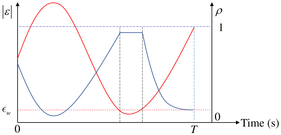
Based on this reformulation, the proposed online ILCCf framework performs real-time learning updates and consists of two primary tasks: (i) executing the online ILCC algorithm in real time, and (ii) designing a fuzzy decision mechanism to regulate convergence parameters. The overall structure of online ILCCf follows the conventional online ILCC architecture [27], with details of the baseline algorithm omitted here. This paper focuses on the fuzzy-regulated convergence strategy, which adaptively adjusts the convergence parameters according to the magnitude of each component of the equivalent contour error. Specifically, large errors are assigned smaller convergence parameters to accelerate learning, while small errors near the steady-state limit use larger parameters to suppress oscillations and prevent divergence, as illustrated in Figure 1. Two regulation schemes are investigated: (1) independent multi-parameter regulation (online ILCCf_i) and (2) unified single-parameter regulation (online ILCCf_u).

3.2. Method 1: Independent Multi-Parameter Convergence Regulation for Online ILCCf

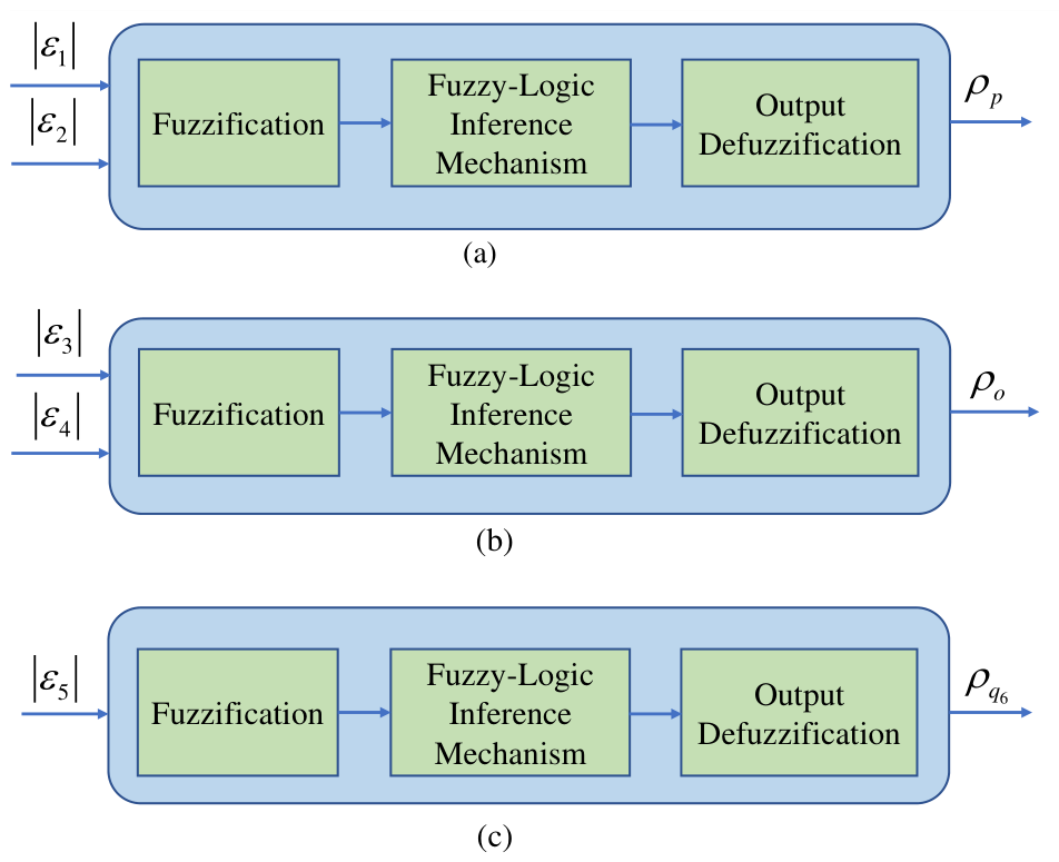
In this method, referred to as online ILCCf_i, three independent Mamdani-type fuzzy inference systems (FISs) are constructed to generate the convergence parameters. These correspond to the position-related components, the orientation-related components, and the sixth-joint-related component of the equivalent contour error. As illustrated in Figure 2a, Figure 2b, and Figure 2c, each FIS is designed for one of these components, respectively. Accordingly, three independent convergence parameters, denoted by ${\rho }_p\left(k\right)$, ${\rho }_o\left(k\right)$, and ${\rho }_{q_6}\left(k\right)$, are obtained. Therefore, in this case, the convergence matrix at each sampling time, ${\Theta }_j\left(k\right)$ in (35), is established as ${\Theta }_j\left(k\right)=\mathrm{diag}\left({\rho }_p\left(k\right),{\rho }_p\left(k\right),{\rho }_o\left(k\right),{\rho }_o\left(k\right),{\rho }_{q_6}\left(k\right)\right)$.

Each FIS adopts a low-dimensional input structure. Specifically, two inputs are used for the position-related and orientation-related components, respectively, whereas a single input is used for the sixth-joint-related component. As a result, the number of fuzzy rules required in each subsystem is significantly reduced and the overall rule base remains compact. A Mamdani-type fuzzy inference structure is adopted owing to its intuitive rule formulation and convenient design procedure.

3.2.1. Mamdani Fuzzy Inference System for Position-Related Components

The proposed fuzzy inference system takes the two position-related equivalent contour error components, ${\epsilon }_{p_1}\left(k\right)$ and ${\epsilon }_{p_2}\left(k\right)$, as inputs and produces a convergence parameter ${\rho }_p\left(k\right)$. The universes of discourse of the input variables are defined as

$${\epsilon }_{p_1}\left(k\right)\in \left[0,{\epsilon }_{p_1}^{max}\right],{\epsilon }_{p_2}\left(k\right)\in \left[0,{\epsilon }_{p_2}^{max}\right],$$

(38)

where ${\epsilon }_{p_1}^{max}$ and ${\epsilon }_{p_2}^{max}$ are selected based on the maximum expected magnitudes of the corresponding equivalent contour error components. The input variables are fuzzified using appropriately defined membership functions, whose number and shape are selected according to design and tuning requirements.

The output variable ${\rho }_p\left(k\right)$ is defined on the interval $[0,1]$. Based on practical considerations, the effective operating range of the convergence parameter is restricted to ${\rho }_p\left(k\right)\in [{\rho }_{min},{\rho }_{max}]$. In general, a larger value of ${\rho }_p\left(k\right)$ (e.g., ${\rho }_p\left(k\right)={\rho }_{max}$) results in a more conservative learning update, whereas a smaller value (e.g., ${\rho }_p\left(k\right)={\rho }_{min}$) leads to a more aggressive update, potentially increasing the risk of over-learning. Accordingly, the output universe of discourse is defined as $[{\rho }_{min},{\rho }_{max}]$, and the variable is represented using appropriately designed membership functions. The number, shape, and distribution of these membership functions are selected based on design requirements and tuning considerations. The n-th fuzzy rule is expressed as

$${\mathcal{R}}_n:\mathrm{IF}{\epsilon }_{p_1}\left(k\right)\mathrm{is}{A}_i\mathrm{AND}{\epsilon }_{p_2}\left(k\right)\mathrm{is}{B}_j\mathrm{THEN}{\rho }_p\left(k\right)\mathrm{is}{C}_{m(i,j)},$$

(39)

where $A_i$ and $B_j$ denote the linguistic terms of the input variables ${\epsilon }_{p_1}\left(k\right)$ and ${\epsilon }_{p_2}\left(k\right)$, respectively, and $C_{m(i,j)}$ denotes the linguistic term of the output variable ${\rho }_p\left(k\right)$. The indices i and j correspond to the selected membership functions of the inputs, and the mapping $m(i,j)$ assigns the corresponding output linguistic term. The total number of rules, denoted by $N_r$, depends on the chosen partitioning of the input spaces.

The firing strength of the n-th rule is computed using the product t-norm as

$${\mu }_n={\mu }_{A_i}\left({\epsilon }_{p_1}\left(k\right)\right){\mu }_{B_j}\left({\epsilon }_{p_2}\left(k\right)\right).$$

(40)

Using the product implication operator, the implied output fuzzy set of the n-th rule is given by

$${\mu }_{C_n}^{\mathrm{imp}}\left(\rho \right)={\mu }_n{\mu }_{C_{m(i,j)}}\left(\rho \right),\forall \rho \in [{\rho }_{min},{\rho }_{max}].$$

(41)

The overall output fuzzy set is obtained by aggregation as

$${\mu }_{\mathrm{out}}\left(\rho \right)={\displaystyle \sum _{n=1}^{N_r}}{\mu }_{C_n}^{\mathrm{imp}}\left(\rho \right),$$

(42)

where $N_r$ denotes the total number of fuzzy rules determined by the selected membership functions. The final convergence parameter is obtained using the centroid defuzzification method as

$${\rho }_p\left(k\right)={\displaystyle \frac{{\displaystyle {\int }_{{\rho }_{min}}^{{\rho }_{max}}\rho {\mu }_{\mathrm{out}}\left(\rho \right)\mathrm{d}\rho }}{{\displaystyle {\int }_{{\rho }_{min}}^{{\rho }_{max}}{\mu }_{\mathrm{out}}\left(\rho \right)\mathrm{d}\rho }}}.$$

(43)

3.2.2. Mamdani Fuzzy Inference System for Orientation-Related Components

A Mamdani-type fuzzy inference system is employed to regulate the convergence parameter associated with the orientation-related components of the equivalent contour error. The overall structure of the fuzzy inference system includes the membership functions, rule base, inference mechanism, aggregation strategy, and defuzzification method. It follows the same formulation as that used for the position-related components.

Specifically, the two orientation-related equivalent contour error components ${\epsilon }_{o_1}\left(k\right)$ and ${\epsilon }_{o_2}\left(k\right)$ are used as inputs, and a single convergence parameter ${\rho }_o\left(k\right)$ is generated as the output. The universes of discourse of the input variables are defined as

$${\epsilon }_{o_1}\left(k\right)\in \left[0,{\epsilon }_{o_1}^{max}\right],{\epsilon }_{o_2}\left(k\right)\in \left[0,{\epsilon }_{o_2}^{max}\right],$$

(44)

where ${\epsilon }_{o_1}^{max}$ and ${\epsilon }_{o_2}^{max}$ are selected based on the maximum expected magnitudes of the corresponding orientation-related equivalent contour error components. The input variables are fuzzified using appropriately designed membership functions, whose number and shape are determined according to design and tuning requirements.

The output variable ${\rho }_o\left(k\right)$ denotes the convergence parameter for the orientation-related learning update and is defined on the interval $[0,1]$. Its effective operating range is restricted to ${\rho }_o\left(k\right)\in [{\rho }_{min},{\rho }_{max}]$. Accordingly, the output universe of discourse is defined as $[{\rho }_{min},{\rho }_{max}]$, and the variable is represented using suitably designed membership functions. The number, shape, and distribution of these membership functions are selected based on design requirements and tuning considerations. All remaining components of the Mamdani fuzzy inference system follow the same design and computational procedures as those described for the position-related components.

3.2.3. Mamdani Fuzzy Inference System for $q_6$-Related Component

This subsection presents a Mamdani-type fuzzy inference system for regulating the convergence parameter associated with the $q_6$-related component of the equivalent contour error. The proposed fuzzy inference system takes the $q_6$-related equivalent contour error component ${\epsilon }_{q_6}\left(k\right)$ as the input and produces the corresponding convergence parameter ${\rho }_{q_6}\left(k\right)$ as the output. The universe of discourse of the input variable is defined as

$$0\le {\epsilon }_{q_6}\left(k\right)\le {\epsilon }_{q_6}^{max},$$

(45)

where ${\epsilon }_{q_6}^{max}$ is selected based on the maximum expected magnitude of the $q_6$-related equivalent contour error component. The input variable is fuzzified using appropriately designed membership functions.

The output variable ${\rho }_{q_6}\left(k\right)$ is defined on the interval $[{\rho }_{min},{\rho }_{max}]$. The variable is represented using suitably designed membership functions, whose number and shape are determined according to design and tuning requirements. The n-th fuzzy rule is written as

$${\mathcal{R}}_n:\mathrm{IF}{\epsilon }_{q_6}\left(k\right)\mathrm{is}{A}_i\mathrm{THEN}{\rho }_{q_6}\left(k\right)\mathrm{is}{C}_{m\left(i\right)},i=1,\dots ,N_r.$$

(46)

The firing strength of the n-th rule is computed as

$${\mu }_n={\mu }_{A_i}\left({\epsilon }_{q_6}\left(k\right)\right).$$

(47)

Using the product implication operator, the implied output fuzzy set is given by

$${\mu }_{C_n}^{\mathrm{imp}}\left(\rho \right)={\mu }_n{\mu }_{C_{m\left(i\right)}}\left(\rho \right),\forall \rho \in [{\rho }_{min},{\rho }_{max}].$$

(48)

The overall output fuzzy set is obtained by aggregation as

$${\mu }_{\mathrm{out}}\left(\rho \right)={\displaystyle \sum _{n=1}^{N_r}}{\mu }_{C_n}^{\mathrm{imp}}\left(\rho \right).$$

(49)

Finally, the convergence parameter associated with the $q_6$-related component is obtained via centroid defuzzification as

$${\rho }_{q_6}\left(k\right)={\displaystyle \frac{{\displaystyle {\int }_{{\rho }_{min}}^{{\rho }_{max}}\rho {\mu }_{\mathrm{out}}\left(\rho \right)\mathrm{d}\rho }}{{\displaystyle {\int }_{{\rho }_{min}}^{{\rho }_{max}}{\mu }_{\mathrm{out}}\left(\rho \right)\mathrm{d}\rho }}}.$$

(50)

3.3. Method 2: Unified Single-Parameter Convergence Regulation for Online ILCCf

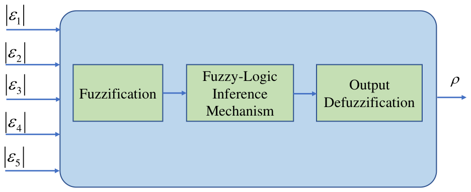
A single fuzzy inference system with five inputs and one output is employed to generate a unified convergence parameter. This approach is referred to as online ILCCf_u, as illustrated in Figure 3. Therefore, the convergence matrix at each sampling time, ${\Theta }_j\left(k\right)$ in (35), is defined as ${\Theta }_j\left(k\right)=\mathrm{diag}\left(\rho \left(k\right),\rho \left(k\right),\rho \left(k\right),\rho \left(k\right),\rho \left(k\right)\right)$. If a Mamdani-type fuzzy inference system were directly constructed for the five input variables, the resulting rule base would become computationally intractable for real-time implementation. Therefore, a zero-order Sugeno-type fuzzy inference structure is adopted to reduce the rule-base size and computational complexity.

The universes of discourse of the five input variables are defined as ${\epsilon }_{p_1}\left(k\right)\in \left[0,{\epsilon }_{p_1}^{max}\right]$, ${\epsilon }_{p_2}\left(k\right)\in \left[0,{\epsilon }_{p_2}^{max}\right]$, ${\epsilon }_{o_1}\left(k\right)\in \left[0,{\epsilon }_{o_1}^{max}\right]$, ${\epsilon }_{o_2}\left(k\right)\in \left[0,{\epsilon }_{o_2}^{max}\right]$, and ${\epsilon }_{q_6}\left(k\right)\in \left[0,{\epsilon }_{q_6}^{max}\right]$. A zero-order Sugeno fuzzy model is adopted. The input variables are fuzzified using appropriately designed membership functions, whose number and shape are determined according to design and tuning requirements. The output variable ${\rho }_j\left(k\right)$ is defined on the interval $[{\rho }_{min},{\rho }_{max}]$ and is represented by constant consequents associated with the fuzzy rule base.

Each fuzzy rule of the proposed Sugeno inference system is formulated as

$${\mathrm{R}}_n:\left\{\begin{array}{c}\mathrm{If}{\epsilon }_{p_1}\left(k\right)\mathrm{is}{A}_1^n\mathrm{and}{\epsilon }_{p_2}\left(k\right)\mathrm{is}{A}_2^n\mathrm{and}{\epsilon }_{o_1}\left(k\right)\mathrm{is}{A}_3^n,\hfill \\ {\epsilon }_{o_2}\left(k\right)\mathrm{is}{A}_4^n\mathrm{and}{\epsilon }_{q_6}\left(k\right)\mathrm{is}{A}_5^n,\hfill \\ \mathrm{then}{\rho }_j\left(k\right)=c_n,\hfill \end{array}\right.$$

(51)

where $A_m^n$ denotes the antecedent linguistic label of the m-th input variable in the n-th rule, and $c_n$ is the corresponding constant consequent.

The firing strength of the n-th rule at iteration k is computed using the product t-norm as

$$w_n\left(k\right)={\displaystyle \prod _{m=1}^{N_r}}{\mu }_{A_m^n}\left({\epsilon }_m\left(k\right)\right),$$

(52)

with ${\epsilon }_1={\epsilon }_{p_1}\left(k\right)$, ${\epsilon }_2={\epsilon }_{p_2}\left(k\right)$, ${\epsilon }_3={\epsilon }_{o_1}\left(k\right)$, ${\epsilon }_4={\epsilon }_{o_2}\left(k\right)$, and ${\epsilon }_5={\epsilon }_{q_6}\left(k\right)$. The unified convergence parameter is obtained by weighted-average defuzzification as

$${\rho }_j\left(k\right)={\displaystyle \frac{{\displaystyle {\displaystyle \sum _{n=1}^{N_r}}{w}_n\left(k\right)c_n}}{{\displaystyle {\displaystyle \sum _{n=1}^{N_r}}{w}_n\left(k\right)}}}.$$

(53)

3.4. Convergence Analysis of the Online ILCCf Scheme

The proposed online ILCCf scheme is developed based on the online ILCC framework in [27] to enable real-time learning. Accordingly, the learning gain matrix $L_j$ is not computed in full; instead, only $N_e$ elements in each column are considered. This reflects the fact that, at each sampling instant k, only the $(k+1)$-th row of $L_j$ is updated, with at most $N_e$ nonzero block elements. The following analysis partially follows the methodology in [27], and readers are referred to that work for further details.

Therefore, consider the lifted equivalent contour error dynamics of the proposed online ILCCf scheme

$${\underline{\epsilon }}_{j+1}=Q_{N_e,j}{\underline{\epsilon }}_j,Q_{N_e,j}=I+{\Gamma }_{j}P{L}_{N_e,j},$$

(54)

where $L_{N_e,j}$ denotes the truncated learning gain matrix with at most $N_e$ effective elements in each column. In contrast to the conventional single-rate design, the proposed learning gain matrix is constructed such that the full learning operator satisfies

$$Q_j=I+{\Gamma }_{j}P{L}_j=\mathrm{diag}\{{\Theta }_j\left(1\right),\dots ,{\Theta }_j\left(T\right)\}$$

(55)

where ${\Theta }_j\left(k\right)=\mathrm{diag}({\rho }_{p_1,j}\left(k\right),{\rho }_{p_2,j}\left(k\right),{\rho }_{o_1,j}\left(k\right),{\rho }_{o_2,j}\left(k\right),{\rho }_{q_6,j}\left(k\right)).$ The diagonal matrix ${\Theta }_j\left(k\right)$ is generated online at each sampling instant k by the fuzzy regulator, using either independent multi-parameter or unified single-parameter regulation. In independent multi-parameter regulation, the convergence parameters are grouped as ${\rho }_{p_1,j}\left(k\right)={\rho }_{p_2,j}\left(k\right)={\rho }_{p,j}\left(k\right)$ and ${\rho }_{o_1,j}\left(k\right)={\rho }_{o_2,j}\left(k\right)={\rho }_{o,j}\left(k\right)$, while ${\rho }_{q_6,j}\left(k\right)$ is regulated independently. In unified single-parameter regulation, a single parameter is applied to all components, ${\rho }_{p_1,j}\left(k\right)={\rho }_{p_2,j}\left(k\right)={\rho }_{o_1,j}\left(k\right)={\rho }_{o_2,j}\left(k\right)={\rho }_{q_6,j}\left(k\right)={\rho }_j\left(k\right)$. In general, the convergence parameters ${\rho }_{p_1,j}\left(k\right)$, ${\rho }_{p_2,j}\left(k\right)$, ${\rho }_{o_1,j}\left(k\right)$, ${\rho }_{o_2,j}\left(k\right)$, and ${\rho }_{q_6,j}\left(k\right)$ are generated online and naturally vary with the iteration index j. For convenience, define

$${\overline{\rho }}_j\triangleq max\left\{{\rho }_{p_1,j}\left(k\right),{\rho }_{p_2,j}\left(k\right),{\rho }_{o_1,j}\left(k\right),{\rho }_{o_2,j}\left(k\right),{\rho }_{q_6,j}\left(k\right)\right\}.$$

(56)

The objective of this subsection is to establish sufficient conditions under which ${\underline{\epsilon }}_j$ converges monotonically for sufficiently large $N_e$.

3.4.1. Boundedness of Jacobian and Learning Gain Matrix

Recall the Jacobian of the path mapping as

$$J_j\left(k\right)={\displaystyle \frac{\partial p\left(y_j\left(k\right)\right)}{\partial y}}.$$

(57)

Assume that the path function $p(·)$ is continuously differentiable and $y_j\left(k\right)$ evolves in a compact set. Hence, the lifted Jacobian ${\Gamma }_j=\mathrm{diag}\{J_j\left(1\right),\dots ,J_j\left(T\right)\}$ is uniformly bounded, i.e.,

$$\parallel {\Gamma }_j\parallel \le \overline{J},\forall j.$$

(58)

The learning gain matrix $L_j$ is computed according to (36) and (37) using the diagonal convergence matrix ${\Theta }_j$. Since the fuzzy regulators generate bounded convergence parameters,

$$0<\underline{\rho }\le {\rho }_{\ell ,j}\left(k\right)\le \overline{\rho }<1,\ell \in \{p_1,p_2,o_1,o_2,q_6\},$$

(59)

and $J_j\left(k\right)$ is bounded, it follows, by the same arguments as in the single-rate case, that $\parallel L_j\parallel$ is uniformly bounded by a constant $\overline{L}$.

3.4.2. Effect of Truncation

Define the truncation-induced perturbation

$$\Delta Q_j\triangleq Q_{N_e,j}-Q_j={\Gamma }_{j}P(L_{N_e,j}-L_j).$$

(60)

Let $P_{\mathrm{tail}}$ denote the truncated portion of P corresponding to the elements beyond the $N_e$-th term, i.e., $P_{\mathrm{tail}}=P-P_{N_e}$. By submultiplicativity of induced norms,

$$\parallel \Delta Q_j\parallel \le \parallel {\Gamma }_j\parallel \parallel P_{\mathrm{tail}}\parallel \parallel L_j\parallel .$$

(61)

Due to the exponential decay of the closed-loop dynamics,

$$\parallel P_{\mathrm{tail}}\parallel \le {\displaystyle \sum _{s=N_e+1}^{\infty }}M{\lambda }^s={\displaystyle \frac{M{\lambda }^{N_e+1}}{1-\lambda }},0<\lambda <1.$$

(62)

Hence, there exists a constant $C>0$ such that

$$\parallel \Delta Q_j\parallel \le C{\lambda }^{N_e+1},C={\displaystyle \frac{\overline{J}\overline{L}M}{1-\lambda }}.$$

(63)

3.4.3. Choice of $N_e$ for Contraction Under Multi-Rate Convergence

The truncated operator can be written as

$$Q_{N_e,j}=Q_j+\Delta Q_j.$$

(64)

From (31) and (35), the induced norm of the full operator satisfies

$$\parallel Q_j\parallel =\parallel {\Theta }_j\parallel ={\overline{\rho }}_j.$$

(65)

Therefore,

$$\parallel Q_{N_e,j}\parallel \le {\overline{\rho }}_j+C{\lambda }^{N_e+1}.$$

(66)

A sufficient condition for monotonic convergence of the lifted equivalent contour error is

$$\parallel Q_{N_e,j}\parallel <1,$$

(67)

which is guaranteed if

$${\overline{\rho }}_j+C{\lambda }^{N_e+1}<1.$$

(68)

Since the fuzzy regulators ensure that ${\overline{\rho }}_j\le \overline{\rho }<1$ for all j, a sufficient iteration-independent choice of $N_e$ is

$$N_e\ge ⌈{\displaystyle \frac{ln\left(\frac{1-\overline{\rho }}{C}\right)}{ln\lambda }}-1⌉.$$

(69)

3.4.4. Boundedness of Equivalent Contour Error

Recalling the lifted equivalent contour error dynamics

$${\underline{\epsilon }}_{j+1}=\underset{U_j}{\underbrace{{\Gamma }_j\left(O_t{\delta }_{j+1}x\left(0\right)+V{\delta }_{j+1}\underline{v}+{\delta }_{j+1}\underline{w}\right)}}+Q_{N_e,j}{\underline{\epsilon }}_j,$$

(70)

taking norms yields

$$\parallel {\underline{\epsilon }}_{j+1}\parallel \le {ϵ}_u+{ϵ}_v+{ϵ}_w+\parallel Q_{N_e,j}\parallel \parallel {\underline{\epsilon }}_j\parallel ,$$

(71)

where ${ϵ}_u={max}_j\parallel {\Gamma }_j{O}_t{\delta }_{j+1}x\left(0\right)\parallel$, ${ϵ}_v={max}_j\parallel {\Gamma }_{j}V{\delta }_{j+1}\underline{v}\parallel$, ${ϵ}_w={max}_j\parallel {\Gamma }_j{\delta }_{j+1}\underline{w}\parallel$. Using (67), the recursion can be unrolled as

$$\parallel {\underline{\epsilon }}_j\parallel \le {\displaystyle \prod _{i=0}^{j-1}}\parallel Q_{N_e,i}\parallel \parallel {\underline{\epsilon }}_0\parallel +{\displaystyle \sum _{n=0}^{j-1}}\left({\displaystyle \prod _{i=n+1}^{j-1}}\parallel Q_{N_e,i}\parallel \right)({ϵ}_u+{ϵ}_v+{ϵ}_w).$$

(72)

Since $\parallel Q_{N_e,i}\parallel \le \overline{\rho }+C{\lambda }^{N_e+1}\triangleq \tilde{\rho }<1,$ it follows that

$$\underset{j\to \infty }{lim\; sup}\parallel {\underline{\epsilon }}_j\parallel \le {\displaystyle \frac{{ϵ}_u+{ϵ}_v+{ϵ}_w}{1-\tilde{\rho }}}.$$

(73)

3.4.5. Concluding Remark

Therefore, if the truncation length $N_e$ satisfies (69), the truncated learning operator $Q_{N_e,j}$ is a strict contraction for all iterations, even in the presence of iteration-varying and componentwise convergence parameters generated by the fuzzy regulators. As a result, the proposed online ILCCf guarantees monotonic convergence of the lifted equivalent contour error.

4. Experimental Validation and Comparison

4.1. System Dynamics and Kinematics

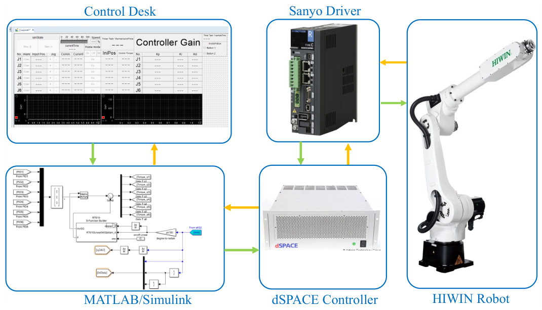
The proposed online ILCCf scheme and the benchmark methods are experimentally evaluated on a commercial six-axis industrial robot (RA610, HIWIN Technologies, Taichung, Taiwan), which is identical to the platform reported in [23]. The built-in robot controller is bypassed and replaced by a PC-based real-time control system composed of a host computer running MATLAB/Simulink 2017b, dSPACE ControlDesk, and a DS1007 digital signal processor. The overall experimental configuration is shown in Figure 4.

The kinematic and dynamic parameters of the robot links are obtained through a standard identification procedure, whose details are omitted for brevity. The identified parameters are then used to establish the continuous-time state-space model in (1). The joint-space proportional and derivative feedback gain matrices in (3) are selected as $K_p=\mathrm{diag}(185,210,160,420,14500,290000),$$K_d=\mathrm{diag}(1,2,1.5,0.7,55,250),$ which determine the closed-loop dynamics in (4). The resulting continuous-time closed-loop model is discretized using a zero-order hold with a sampling period of $1\mathrm{ms}$, leading to the discrete-time system matrices A, B, and C required for the implementation of the online ILCCf algorithm. The explicit expressions of these matrices are omitted for brevity.

The desired motion is specified by a Cartesian position trajectory together with a corresponding end-effector orientation trajectory. Let $P={[P_x,P_y,P_z]}^{\top }\in {\mathbb{R}}^3$ denote the Cartesian position vector, and let $O={[O_x,O_y,O_z]}^{\top }\in {\mathbb{R}}^3$ denote a unit vector describing the end-effector orientation. For the considered robot, the mapping from the joint coordinate vector q to the task-space variables is given by

$$(P,O)=f\left(q\right),$$

(74)

where $f(·)$ denotes the forward kinematic transformation determined by the robot geometry. Conversely, the joint coordinates associated with a prescribed position and orientation are obtained through the inverse kinematics,

$$q=f^{-1}(P,O).$$

(75)

4.2. Trajectory Design and Establishment of the Equivalent Contour Error

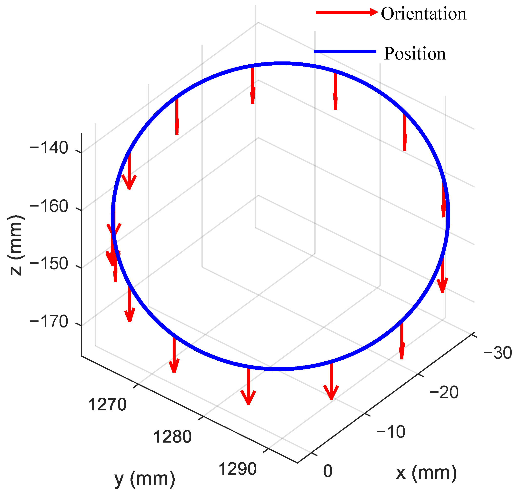
As shown in Figure 5, the reference path is a spatial circular trajectory defined in the task coordinate system. The circle has a radius of $R=20\mathrm{mm}$ and its center is located at $(c_x,c_y,c_z)=(-14.14214,1278.14214,-153.0)\mathrm{mm}$. The plane of the circle is characterized by a unit normal vector $n=\left(\frac{1}{\sqrt{3}},\frac{1}{\sqrt{3}},\frac{1}{\sqrt{3}}\right)$. The end-effector orientation is kept constant and specified by $O={[0,0,-1]}^{\top }$, meaning that the tool is always oriented downward and no rotational motion about its axis is considered. The translational motion along the path is generated using an S-curve velocity profile, with the maximum feedrate set to $100\mathrm{mm}/\mathrm{s}$.

In order to construct the equivalent contour error, a joint-space path description associated with the desired task-space trajectory is first required. The Cartesian position of the prescribed three-dimensional circular path is parameterized as

$$P_d\left(t\right)=\left[\begin{array}{c}{P}_{dx}\left(t\right)\\ P_{dy}\left(t\right)\\ P_{dz}\left(t\right)\end{array}\right]=\left[\begin{array}{c}{c}_x+Rcos\theta \left(t\right)n_{1x}+Rsin\theta \left(t\right)n_{2x}\\ c_y+Rcos\theta \left(t\right)n_{1y}+Rsin\theta \left(t\right)n_{2y}\\ c_z+Rcos\theta \left(t\right)n_{1z}+Rsin\theta \left(t\right)n_{2z}\end{array}\right],$$

(76)

while the desired end-effector orientation is fixed and given by

$$d_{\left(t\right)}={[O_{dx}\left(t\right),O_{dy}\left(t\right),O_{dz}\left(t\right)]}^{\top }={[0,0,-1]}^{\top }.$$

(77)

Here, $n_1={[n_{1x},n_{1y},n_{1z}]}^{\top }$ and $n_2={[n_{2x},n_{2y},n_{2z}]}^{\top }$ denote two orthonormal vectors spanning the plane of the circle, and $\theta \left(t\right)$ is the scalar path parameter.

Based on the path descriptions in (76) and (77), the equivalent contour error can be formulated in the machine coordinate space. For a six-axis manipulator, five independent constraint functions are required to characterize the contouring deviation. For the positional motion in (76), the circular path can be described equivalently by a geometric plane constraint and a constant-radius constraint, which together yield two algebraic equations. For the fixed orientation, two components of the orientation vector are selected as constraint functions, for instance $O_x\left(q\right)=0$ and $O_z\left(q\right)+1=0$. Furthermore, under the assumption that the tool is not allowed to rotate about its own axis, the sixth joint is constrained directly. Consequently, the equivalent contour error in the machine coordinate system is defined as

$$\epsilon =\left[\begin{array}{c}{(y_x-c_x)}^2+{(y_y-c_y)}^2+{(y_z-c_z)}^2-R^2\\ n_x(y_x-c_x)+n_y(y_y-c_y)+n_z(y_z-c_z)\\ O_x\left(q\right)\\ O_z\left(q\right)+1\\ q_6\end{array}\right].$$

(78)

By substituting the forward kinematic mapping in (74) into (78), the above equivalent contour error can be written explicitly as a function of the machine-axis variables. It is emphasized that the equivalent contour error formulation allows efficient real-time evaluation. This property makes it particularly suitable for the practical implementation of the proposed online ILCCf scheme.

4.3. Settings of the Fuzzy Inference Systems

The closed-loop system in (5) is stable. Therefore, any bounded reference input yields a bounded system response and, consequently, bounded equivalent contour errors. Based on experimental observations, the maximum absolute values of the individual equivalent contour error components are given by $[{\epsilon }_{p_1}^{max},{\epsilon }_{p_2}^{max},{\epsilon }_{o_1}^{max},{\epsilon }_{o_2}^{max},{\epsilon }_{q_6}^{max}]=\begin{array}{cc}& [2.5\times {10}^{-5},1.2\times {10}^{-3},5.0\times {10}^{-5},1.2\times {10}^{-3},3.1\times {10}^{-4}].\hfill \end{array}$ For simplicity of controller design and to enable a fair comparison between the two fuzzy regulation strategies, online ILCCf_i and online ILCCf_u adopt exactly the same fuzzification settings for both inputs and outputs.

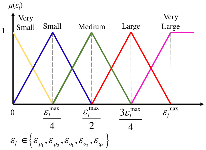
Note that the proposed online ILCCf is implemented in real time with a sampling time of 1 ms. This implies that the computation of both the feedback controller in (2) and the online ILCCf must be completed within 1 ms. According to [27] (using the same system, parameter settings, and trajectory), the computation time of the online ILCC (without fuzzy regulation) on a dSPACE platform is approximately 0.69 ms. Therefore, the computational complexity of the fuzzy inference system must be carefully controlled; otherwise, the total computation time may exceed the 1 ms sampling period, preventing real-time implementation of the proposed ILCCf. To ensure real-time feasibility, triangular membership functions are adopted for both input and output variables. The number of membership functions is selected based on a trade-off between control performance and computational efficiency via trial-and-error. It is observed that using five membership functions provides a satisfactory balance between control performance and computational cost, while a larger number significantly increases computation time.

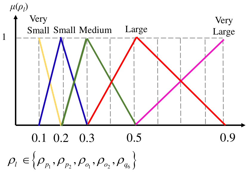
Each input variable is described by symmetric triangular membership functions associated with the linguistic terms $\{\mathrm{VS},\mathrm{S},\mathrm{M},\mathrm{L},\mathrm{VL}\}$, corresponding to very small, small, medium, large, and very large error levels, respectively, as illustrated in Figure 6. These membership functions are uniformly distributed over the input universes of discourse with equal overlap. With this structure, at most two membership functions are activated at any sampling instant, which helps reduce computational burden and is suitable for real-time implementation. The output variable, denoted by ${\rho }_p$, is defined on the interval $[0.1,0.9]$ and is also represented by five triangular membership functions using the same linguistic labels $\{\mathrm{VS},\mathrm{S},\mathrm{M},\mathrm{L},\mathrm{VL}\}$. The centers of the output membership functions are chosen as ${\rho }_p^{\left(m\right)}\in \{0.1,0.3,0.5,0.7,0.9\}$ for $m=1,\dots ,5$, as illustrated in Figure 7.

Note that the convergence parameter represents the closed-loop eigenvalue of the iteration error dynamics, which must be less than one to ensure convergence. The range of the convergence parameter, $[0.1,0.9]$, is selected based on empirical observations and practical considerations. Specifically, when the parameter is smaller than 0.1, the learning update becomes overly aggressive, which may amplify the effects of sensor noise in practice, leading to local divergence. On the other hand, when the parameter is larger than 0.9, the learning process becomes overly conservative, resulting in slow convergence and reduced learning effectiveness. Therefore, the selected range provides a practical trade-off between convergence speed and noise effects.

4.4. Fuzzy Rule Bases for Online ILCCf

The fuzzy rule bases are tuned empirically to achieve optimal control performance. For online ILCCf_i, separate Mamdani-type rule bases are defined for the position-related, orientation-related, and $q_6$-related components, summarized in

Table 1. Mamdani fuzzy rule base for the position-related components in online ILCCf_i.

${\mathit{\epsilon }}_{{\mathit{p}}_1}\setminus {\mathit{\epsilon }}_{{\mathit{p}}_2}$	VS	S	M	L	VL
VS	VL	VL	L	M	M
S	VL	L	M	M	S
M	L	M	M	S	S
L	L	M	S	S	S
VL	M	S	S	S	VS

,

Table 2. Mamdani fuzzy rule base for the orientation-related components in online ILCCf_i.

${\mathit{\epsilon }}_{{\mathit{o}}_1}\setminus {\mathit{\epsilon }}_{{\mathit{o}}_2}$	VS	S	M	L	VL
VS	VL	L	M	M	M
S	L	L	M	M	S
M	L	M	M	S	S
L	L	M	S	S	S
VL	L	M	S	S	VS

and

Table 3. Mamdani fuzzy rule base for the $q_6$-related component in online ILCCf_i.

${\mathit{\epsilon }}_{{\mathit{q}}_6}$	VS	S	M	L	VL
${\rho }_{q_6}$	VL	L	M	S	VS

. For online ILCCf_u, a unified Sugeno-type rule base is employed, as shown in

Table 4. Sugeno-type fuzzy rule base in online ILCCf_u.

Rule	${\mathit{\epsilon }}_1$	${\mathit{\epsilon }}_2$	${\mathit{\epsilon }}_3$	${\mathit{\epsilon }}_4$	${\mathit{\epsilon }}_5$	$\mathit{\rho }$
1	VL	VL	VL	VL	VL	VS
2	L	–	–	–	–	S
3	–	L	–	–	–	S
4	–	–	–	L	–	S
5	M	–	–	–	–	M
6	–	M	–	–	–	M
7	–	–	–	M	–	M
8	S	–	–	–	–	L
9	–	S	–	–	–	L
10	–	–	–	S	–	L
11	VS	VS	–	VS	–	VL

.

4.5. Experimental Setup for Iterative Learning Control

To evaluate the effectiveness of the proposed online ILCCf strategy, experiments are conducted for each prescribed path under the following four control schemes:

• Case 1: online ILCC with a fixed convergence parameter $\rho =0.25$.
• Case 2: online ILCC with a fixed convergence parameter $\rho =0.80$.
• Case 3: online ILCCf_u.
• Case 4: online ILCCf_i.

The performance of the four schemes is evaluated in terms of convergence speed and contouring accuracy, including the maximum position and orientation contour errors at the convergence stage, as well as the corresponding RMS contour errors. For each control scheme, six learning iterations are performed. Together with the baseline trial without learning, a total of seven executions are conducted for each scheme. The number of effective learning gains is set to $N_e=30$. In addition, a low-pass filter with a cutoff frequency of $f_c=50\mathrm{Hz}$ is applied to the encoder signals to suppress measurement noise.

4.6. Experimental Results

4.6.1. Convergence Parameter $\rho$

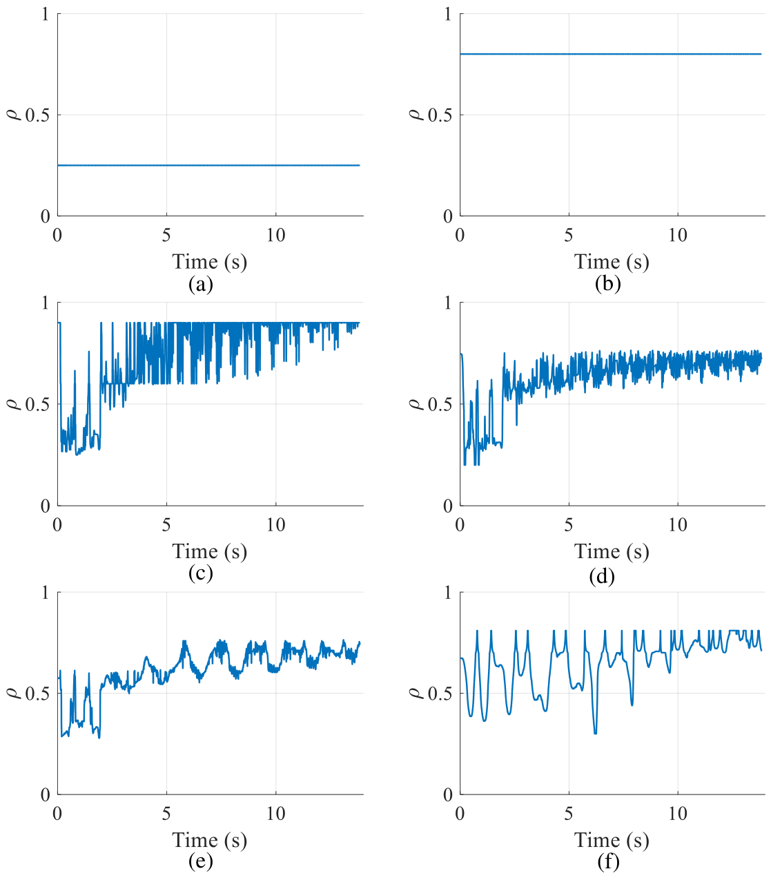
The convergence parameter $\rho$ is plotted continuously over time and across learning iterations in Figure 8. Note that the trajectory period (i.e., the duration of one iteration) is $1.792\mathrm{s}$. Figure 8 shows the results over seven executions, including one baseline iteration without learning and six learning iterations, which corresponds to a total duration of $12.544\mathrm{s}$.

Figure 8a shows the convergence parameter for Case 1, where a constant convergence parameter $\rho =0.25$ is used. Figure 8b shows the convergence parameter for Case 2, where a constant convergence parameter $\rho =0.80$ is adopted. Figure 8c shows the convergence parameter for Case 3. In this case, the five components of the equivalent contour error are used as inputs to generate a single convergence parameter $\rho$. Since the same convergence parameter is applied to all components of the equivalent contour error, all components in (32) share an identical convergence parameter. It can be observed that, at the baseline iteration without learning, $\rho$ is evaluated to be relatively small, corresponding to a fast learning rate (note that the convergence parameter computed at the current iteration is used to generate the control command for the next iteration). In the subsequent learning iterations, $\rho$ increases gradually and converges toward the predefined upper bound (0.9) as the equivalent contour error decreases. This behavior indicates that the fuzzy controller is able to regulate the convergence parameter properly according to the magnitude of the equivalent contour error.

The convergence parameters for Case 4 are shown in Figure 8d–f. Three independent Mamdani fuzzy controllers are employed to regulate the convergence parameters for different error components. The controller for the position contour error uses the position component of the equivalent contour error to determine its convergence parameter (Figure 8d), while the controller for the orientation contour error uses the orientation component (Figure 8e). Additionally, a separate controller regulates the $q_6$ motion based on its corresponding error component (Figure 8f).

It can be clearly observed that the convergence parameters for the position, orientation, and $q_6$ components, denoted as ${\rho }_p$, ${\rho }_o$, and ${\rho }_{q6}$, are relatively small at the baseline iteration without learning, which is used to generate the control commands for the first learning iteration. As learning progresses and the equivalent contour error gradually decreases over iterations (see Figure 9 and Figure 10), the convergence parameters increase accordingly for all three components. This behavior indicates that a fast learning rate is applied when the contour error is large, while a slower learning rate is adopted as the error diminishes, thereby preventing over-learning and potential divergence.

4.6.2. RMS Position and Orientation Contour Error

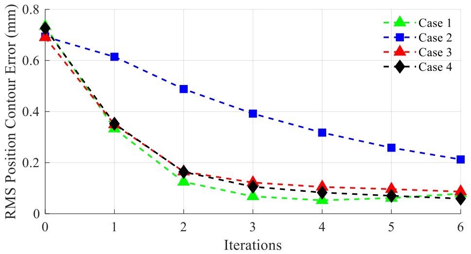
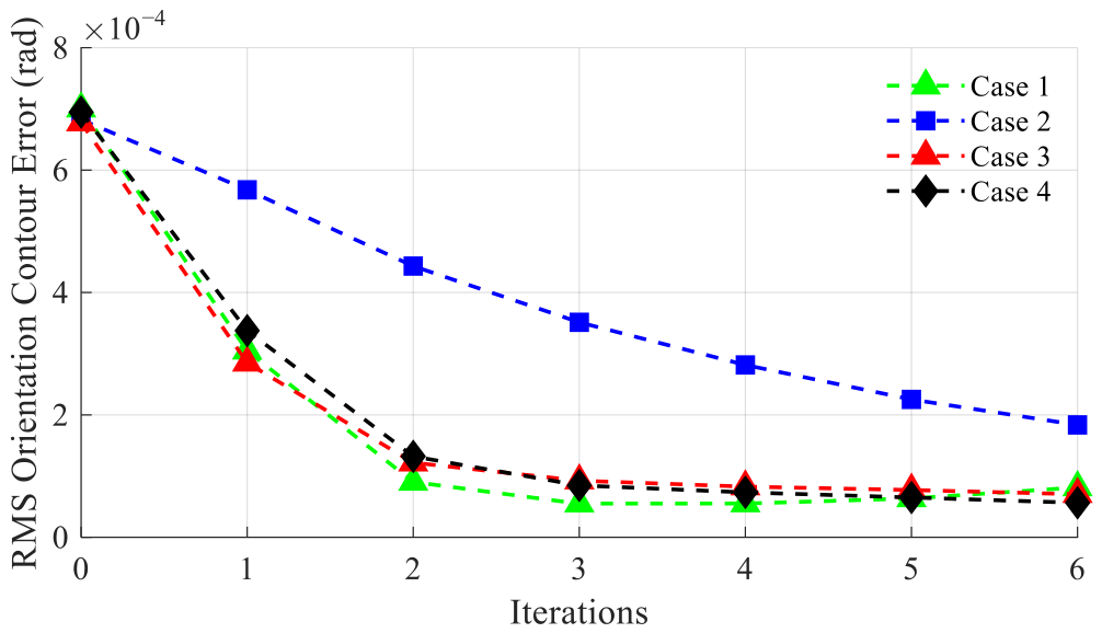
For comparison, the RMS position contour errors of all cases are plotted in the same figure in Figure 9, and the corresponding RMS orientation contour errors are shown in Figure 10. For Case 1 (fixed $\rho =0.25$), the RMS position contour error is reduced from $7.3379\times {10}^{-1}\mathrm{mm}$ to $5.2694\times {10}^{-2}\mathrm{mm}$ at the 4th learning iteration, while the RMS orientation contour error is reduced from $7.0043\times {10}^{-4}\mathrm{rad}$ to $5.5019\times {10}^{-5}\mathrm{rad}$ at the 3rd learning iteration. For Case 2 (fixed $\rho =0.80$), the RMS position contour error decreases from $6.9328\times {10}^{-1}\mathrm{mm}$ to $2.1246\times {10}^{-1}\mathrm{mm}$ at the 6th learning iteration, and the RMS orientation contour error decreases from $6.8253\times {10}^{-4}\mathrm{rad}$ to $1.8363\times {10}^{-4}\mathrm{rad}$ at the 6th learning iteration. For Case 3 (online ILCCf_u), the RMS position contour error decreases from $6.9033\times {10}^{-1}\mathrm{mm}$ to $8.6610\times {10}^{-2}\mathrm{mm}$ at the 6th learning iteration, and the RMS orientation contour error decreases from $6.7775\times {10}^{-4}\mathrm{rad}$ to $7.0450\times {10}^{-5}\mathrm{rad}$ at the 6th learning iteration. For Case 4 (online ILCCf_i), the RMS position contour error decreases from $7.2625\times {10}^{-1}\mathrm{mm}$ to $5.9251\times {10}^{-2}\mathrm{mm}$ at the 6th learning iteration, and the RMS orientation contour error decreases from $6.9478\times {10}^{-4}\mathrm{rad}$ to $5.6396\times {10}^{-5}\mathrm{rad}$ at the 6th learning iteration.

Clearly, Case 2 exhibits slow convergence due to the large convergence parameter $\rho =0.80$. Compared with Cases 1, 3, and 4, the learning speed of Case 2 is significantly lower. Consequently, even at the 6th learning iteration, the contour errors of Case 2 remain relatively large and the learning process has not yet fully converged. To achieve smaller contour errors, additional learning iterations would be required. Such slow convergence is undesirable in industrial applications, because more learning iterations directly imply longer setup time and higher production cost, especially in mass-production environments where time efficiency is critical. Therefore, Case 2 is not preferred for practical manufacturing.

For Case 1, the RMS position contour error converges at the 4th learning iteration and the RMS orientation contour error converges at the 3rd learning iteration, after which a slight divergence can be observed. In contrast, Cases 3 and 4 converge at approximately the 6th learning iteration for both the position and orientation contour errors. Overall, Cases 1, 3, and 4 exhibit comparable convergence speeds and achieve similar levels of RMS position and orientation contour errors at their respective convergence iteration. Among all cases, Case 1 achieves the smallest RMS contour errors, followed by Cases 3, 4, and 2. However, although Case 1 yields the smallest RMS errors, its orientation contour error starts to diverge after the 3rd learning iteration, while the position contour error converges at the 4th learning iteration. This indicates that the orientation contour error begins to diverge when the position contour error has already converged, which is undesirable in industrial practice.

Moreover, the aggressive learning setting in Case 1 may induce local divergence, which will be further demonstrated in the next section. By contrast, Cases 3 and 4, which employ fuzzy regulation of the convergence parameter, produce slightly larger RMS contour errors, but offer a more favorable trade-off between convergence speed and robustness by mitigating the risk of local divergence. The slightly larger steady-state errors in Cases 3 and 4 arise because, when the contour error approaches a predefined tolerance region, the convergence parameter is adaptively increased to prevent over-learning and divergence. As a result, the contour errors of the fuzzy-regulated cases converge to a small neighborhood around the desired bound rather than exactly to the bound itself.

4.6.3. Maximum Position and Orientation Contour Errors at the Convergence

This section investigates the position and orientation contour errors in terms of the maximum position and orientation contour errors at the convergence, and further examines the occurrence of local divergence by analyzing the contour errors at each sampling instant and learning iteration.

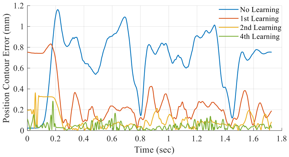
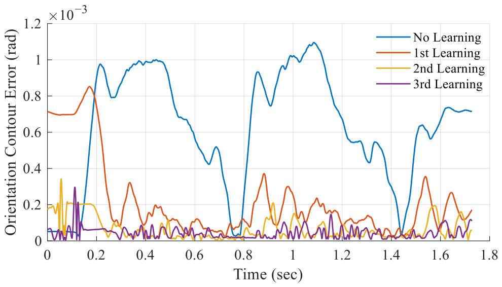
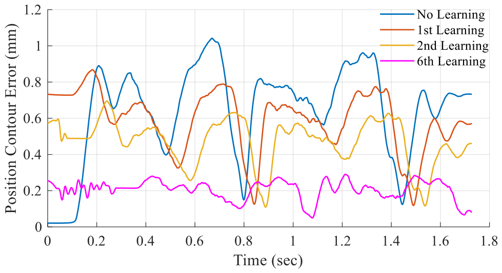
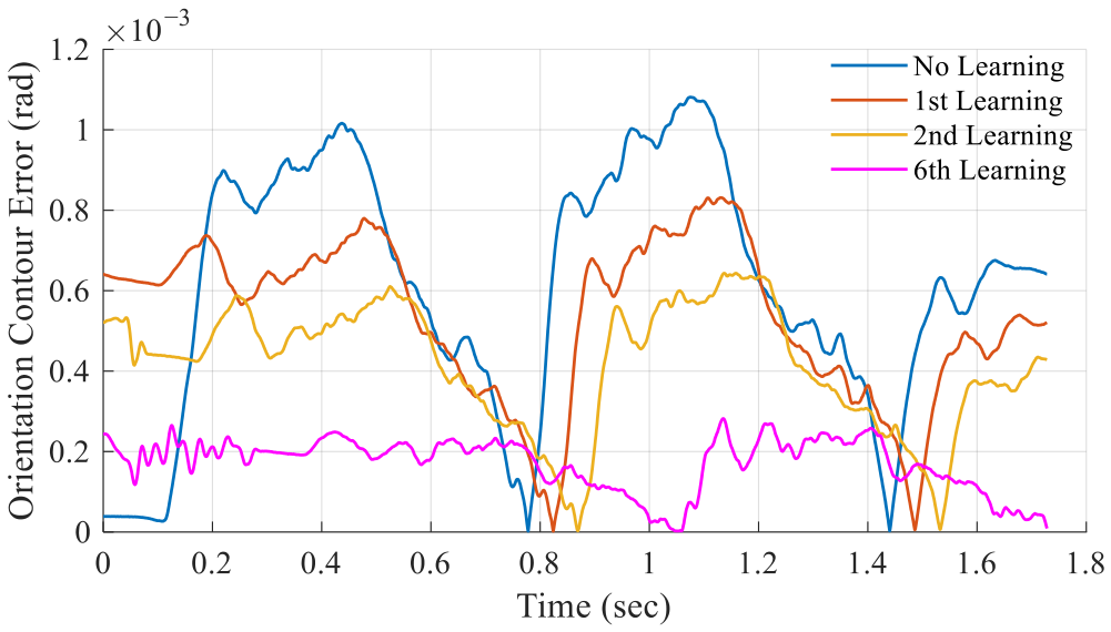
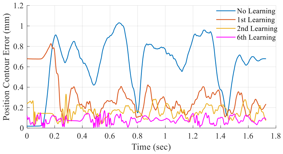
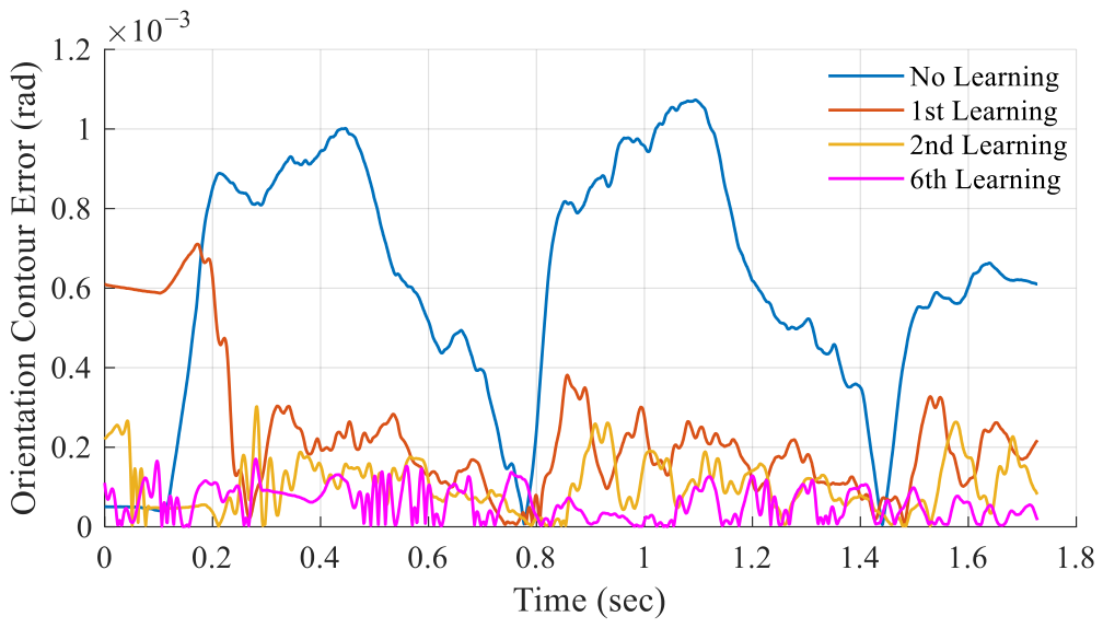
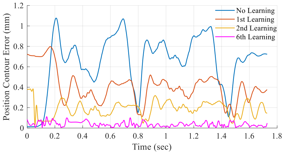
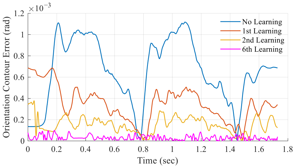
The position and orientation contour errors for Case 1, Case 2, Case 3, and Case 4 are presented in Figure 11 and Figure 12, Figure 13 and Figure 14, Figure 15 and Figure 16, and Figure 17 and Figure 18, respectively. Although six learning iterations are carried out (resulting in seven executions, including the baseline trial without learning), only representative iterations are plotted for clarity. For Case 1, the baseline trial and the 1st, 2nd, and 4th learning iterations (which yield the smallest position contour errors) are shown for the position results, while the baseline trial and the 1st, 2nd, and 3rd learning iterations (which yield the smallest orientation contour errors) are shown for the orientation results. For Cases 2, 3, and 4, the baseline trial and the 1st, 2nd, and 6th learning iterations (which yield the smallest errors) are presented for both the position and orientation contour errors.

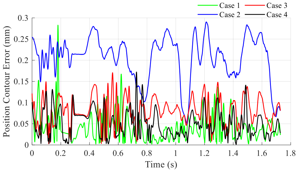
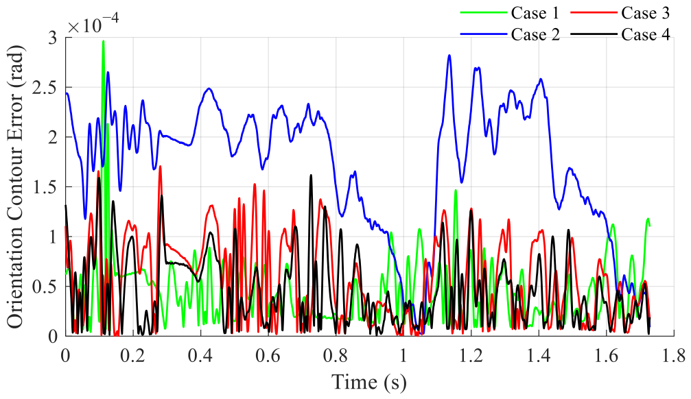
It can be observed that, for all the considered learning schemes, both the position and orientation contour errors decrease monotonically with the learning iteration at nearly every sampling instant. To further compare the contouring performance at convergence, the position and orientation contour errors at the iteration corresponding to the smallest RMS are shown in Figure 19 and Figure 20, respectively. Quantitative comparisons of the maximum contour errors are summarized as follows. For Case 1, the maximum position and orientation errors are reduced from $1.1618\mathrm{mm}$ and $1.0955\times {10}^{-3}\mathrm{rad}$ to $2.8291\times {10}^{-1}\mathrm{mm}$ and $2.9643\times {10}^{-4}\mathrm{rad}$, respectively. For Case 2, they decrease from $1.0420\mathrm{mm}$ and $1.0814\times {10}^{-3}\mathrm{rad}$ to $2.9037\times {10}^{-1}\mathrm{mm}$ and $2.8216\times {10}^{-4}\mathrm{rad}$. For Case 3, the corresponding errors are reduced from $1.0307\mathrm{mm}$ and $1.0731\times {10}^{-3}\mathrm{rad}$ to $1.7066\times {10}^{-1}\mathrm{mm}$ and $1.7075\times {10}^{-4}\mathrm{rad}$. For Case 4, they decrease from $1.1348\mathrm{mm}$ and $1.0859\times {10}^{-3}\mathrm{rad}$ to $1.7234\times {10}^{-1}\mathrm{mm}$ and $1.6186\times {10}^{-4}\mathrm{rad}$.

From visual inspection, it can be clearly observed that Case 2, with a fixed convergence parameter of $\rho =0.80$, exhibits larger position and orientation contour errors at most sampling points compared with Cases 1, 3, and 4. This is mainly due to the large convergence parameter, which leads to a slow learning speed (as discusses previously). Even at the 6th learning iteration, the contour errors of Case 2 remain relatively large when compared with the other cases. In contrast, for Cases 1, 3, and 4, the position and orientation contour errors at their best learning iterations are generally similar over most sampling points. However, in terms of the maximum contour error, Case 2 still yields relatively large maximum position and orientation contour errors because of its slow convergence parameter.

For Case 1, which uses a fixed convergence parameter of $\rho =0.25$ and thus a faster learning speed, although the contour errors at most sampling points are significantly smaller than those of Case 2, the maximum contour errors at the convergence stage remain at a similar level. For example, the maximum position contour errors are $2.8291\times {10}^{-1}\mathrm{mm}$ for Case 1 and $2.9037\times {10}^{-1}\mathrm{mm}$ for Case 2, while the corresponding maximum orientation contour errors are $2.9643\times {10}^{-4}\mathrm{rad}$ for Case 1 and $2.8216\times {10}^{-4}\mathrm{rad}$ for Case 2. Such behavior is generally undesirable in industrial applications.

Although Case 1 adopts a relatively aggressive learning setting, the large learning gain may excite local unstable modes of the learning dynamics. As a result, while most sampling points exhibit good convergence, local divergence can still occur. This phenomenon highlights a critical limitation of using a small convergence parameter (i.e., fast convergence speed), which may lead to local divergence. In practical machining applications, even if the contour errors at most locations are very small, the presence of one or several locations with relatively large errors can significantly deteriorate the overall machining accuracy, making the improvement at other locations less meaningful. Conversely, when a large convergence parameter is used, as in Case 2, the learning speed becomes very slow. These results clearly support the proposed fuzzy decision-making strategy. It adaptively regulates the convergence parameter according to the equivalent contour error, thereby achieving a better trade-off between convergence speed and robustness. For Cases 3 and 4, which employ fuzzy decision systems (online ILCCf_u in Case 3 and online ILCCf_i in Case 4), the achieved minimum contour errors are at nearly the same level. Specifically, the minimum position contour errors are $1.7066\times {10}^{-1}\mathrm{mm}$ for Case 3 and $1.7234\times {10}^{-1}\mathrm{mm}$ for Case 4, while the corresponding minimum orientation contour errors are $1.7075\times {10}^{-4}\mathrm{rad}$ for Case 3 and $1.6186\times {10}^{-4}\mathrm{rad}$ for Case 4.

Compared with Case 1, both Cases 3 and 4 effectively avoid local divergence at the locations where the maximum contour errors occur, while maintaining a comparable convergence speed that is significantly faster than that of Case 2. This indicates that the introduction of a time-varying convergence parameter plays a key role in improving convergence speed while preserving contouring performance. A closer comparison between Cases 3 and 4, however, reveals important differences in local behavior. Although their position and orientation contour errors at the convergence stage (the 6th learning iteration) are nearly identical in terms of minimum values, Case 3 exhibits noticeable oscillations and local divergence within the time interval from $0.45$ s to $0.6$ s for both position and orientation contour errors. In contrast, Case 4 maintains consistently small contour errors without noticeable oscillations over the entire trajectory.

An inspection of the RMS contour errors further shows that, at the 6th learning iteration, Case 3 is still undergoing convergence and exhibits local oscillatory and divergent behavior, which is undesirable for practical machining applications. This phenomenon can be attributed to the use of a single convergence parameter for all components of the equivalent contour error in Case 3. In practice, the position, orientation, and sixth-joint components do not converge synchronously; therefore, enforcing a unified convergence rate for all components is not appropriate. By contrast, Case 4 adopts independent convergence parameters for the position-, orientation-, and $q_6$-related components of the equivalent contour error. Therefore, the independent convergence parameter scheme allows the distinct dynamic characteristics of each component to be properly accommodated, resulting in improved stability, reduced oscillations, and more robust convergence performance.

Overall, these results demonstrate that the proposed fuzzy decision mechanism enables the online ILCCf algorithm to adaptively adjust the convergence rates in real time based on the instantaneous evaluation of the equivalent contour error. In particular, the proposed online ILCCf_i scheme, with independent multi-parameter regulation, achieves the best contouring performance among all tested cases. In summary, the time-varying convergence parameter improves convergence speed and prevents local divergence, while the independent parameter design further enhances robustness, leading to improved contouring performance.

4.6.4. Computation Time

The computation time of the proposed algorithm depends on the hardware platform, which in this study is the dSPACE DS1007 system. Due to limitations of the dSPACE platform, it is not possible to isolate the execution time of individual program modules. Instead, dSPACE ControlDesk provides a parameter referred to as the turnaround time, which represents the total execution time of the entire control program.

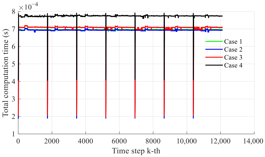
In this study, the measured total execution time includes both the feedback linearization and online ILCC algorithms. Specifically, for Cases 1 and 2, the implementation consists of feedback linearization and the standard online ILCC algorithm, whereas for Cases 3 and 4, it includes feedback linearization and the online ILCCf algorithm. The computation times for Cases 1–4 are illustrated in Figure 21, which presents the execution time over seven iterations. The results clearly indicate that Case 4 exhibits the highest computation time, followed by Case 3. Cases 1 and 2 show similar and comparatively lower computation times.

On average, Case 4 (ILCCf_i) requires 0.7717 ms due to the use of three fuzzy inference systems (for position, orientation, and $q_6$), each consisting of 25 rules. Case 3 (ILCCf_u) requires 0.7042 ms, as it employs a single unified fuzzy system with 11 rules. Case 2 requires 0.6891 ms with a fixed $\rho =0.8$ and no fuzzy inference, while Case 1 uses a fixed $\rho =0.25$ and also does not involve fuzzy logic. Although the execution time of the fuzzy subsystem cannot be directly measured, it can be estimated indirectly. Since Cases 1 and 2 do not include fuzzy computation, their average execution time can be used as a baseline. By subtracting this baseline from the total execution time of Cases 3 and 4, the additional computational cost introduced by the fuzzy systems can be approximated. Based on this approach, the fuzzy computation time is approximately 0.0151 ms for Case 3 and 0.0826 ms for Case 4.

Given a sampling time of 1 ms, although the proposed method incorporates fuzzy systems, the total execution time of the ILCCf algorithm remains below the sampling interval, thus ensuring real-time implementation feasibility.

4.6.5. Discussion

Two fuzzy-based convergence-parameter regulation schemes are investigated within the proposed online ILCCf framework: online ILCCf_i and online ILCCf_u. Both strategies effectively mitigate local divergence caused by improperly selected fixed parameters and improve contouring performance while maintaining comparable convergence speed. In the comparison between online ILCCf_i and online ILCCf_u, online ILCCf_i achieves superior contouring performance. From a design perspective, online ILCCf_i employs three independent fuzzy inference systems for the position, orientation, and $q_6$ motion errors, respectively. This decoupled structure provides a more flexible and intuitive design compared with the unified single-parameter Sugeno fuzzy scheme.

The real-time feasibility of the proposed online ILCCf is enabled by three key components: (i) the online ILCC framework in [27], (ii) a real-time computable equivalent contour error model, and (iii) the fuzzy regulation strategy. In contrast, conventional ILC schemes based on actual contour error models are generally unsuitable for real-time implementation due to the high computational cost of contour error optimization.

5. Additional Validation

The primary experiments in Section 4 focus on performance comparisons with existing methods. This additional validation is conducted to evaluate the robustness of the proposed method under model uncertainty and measurement noise. The same six-axis industrial robot model from HIWIN used in Section 4 is adopted. In the simulation setting, the previously defined parametric uncertainty term $\Delta$ in the closed-loop system dynamics in (4) is activated to represent a 5% modeling error. Measurement noise is modeled as a combination of sinusoidal disturbances and random noise, expressed as

$$w_c\left(t\right)=\left(sin(2\pi ·55t)+sin(2\pi ·65t)+0.8\mathrm{rand}\left(t\right)\right)\times {10}^{-6}.$$

(79)

In addition, encoder quantization is considered based on a 17-bit encoder, consistent with the experimental system. A low-pass filter with a cutoff frequency of 50 Hz is assumed. As a result, the component at 45 Hz is not fully attenuated, which is used to further evaluate the robustness of the proposed method under residual periodic disturbances. Since ILCCf_i has demonstrated superior contouring performance compared with ILCCf_u, only ILCCf_i is considered in this validation. The same reference trajectory as in Section 4 is used.To account for the presence of model uncertainty and noise, the fuzzy inference system is re-tuned accordingly. Two cases are considered in this simulation: Case 5: online ILCC with a fixed convergence parameter $\rho =0.3$; and Case 6: online ILCCf_i.

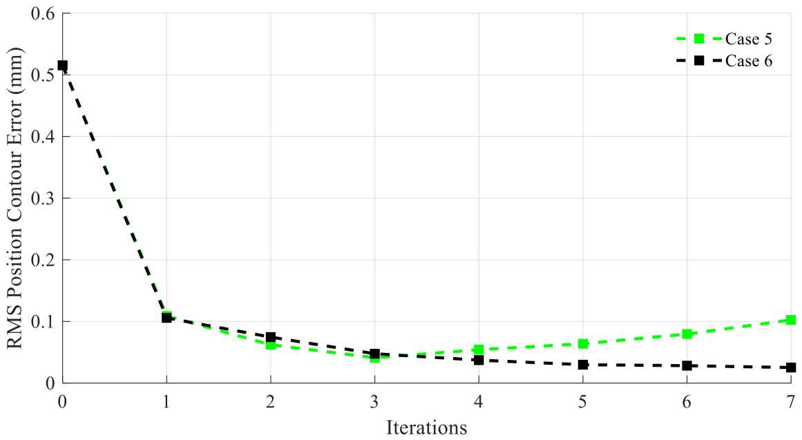
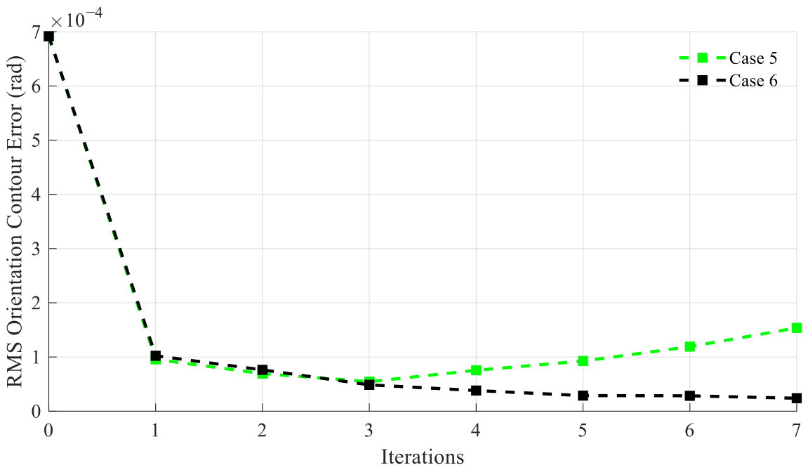
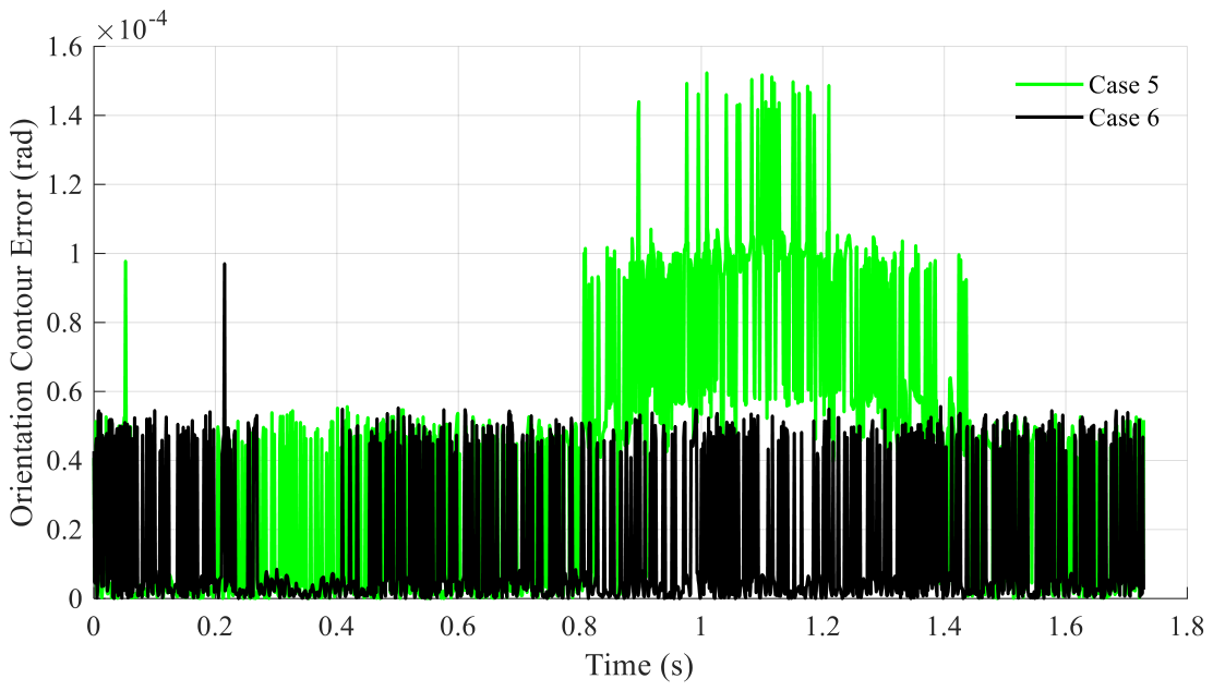
The simulation is conducted over seven learning iterations for each case. Detailed profiles of the position contour error and orientation contour error are omitted here for brevity. The RMS position and orientation contour errors are presented in Figure 22 and Figure 23, respectively. For Case 5, both position and orientation contour errors converge by the third iteration, reaching 0.04112 mm and $5.457\times {10}^{-5}$ rad, respectively, and diverged from the fourth iteration onward. In contrast, for Case 6, the position and orientation contour errors converge more gradually, reaching 0.02521 mm and $2.396\times {10}^{-5}$ rad at the seventh iteration, while still exhibiting a decreasing trend.

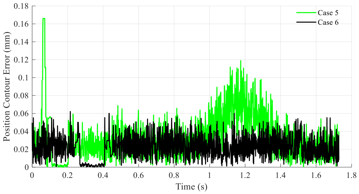
The contour errors at convergence are illustrated in Figure 24 and Figure 25. The results indicate that both Case 5 and Case 6 achieve comparable accuracy at convergence. However, Case 5 exhibits noticeable oscillations around 0.061 s and within the interval 1.0–1.3 s in position, as well as around 0.052 s and within 0.8–1.4 s in orientation. As a result, the position and orientation contour errors in Case 5 are amplified to more than twice their nominal levels in these regions. Therefore, the proposed online ILCCf demonstrates superior contouring performance at convergence by effectively suppressing oscillations.

In general, the proposed online ILCCf shows strong robustness against system uncertainties, model inaccuracies, and measurement noise, enabling faster convergence while maintaining minimal contour errors at convergence.

6. Conclusions

This paper proposes an online ILCC framework with fuzzy-regulated convergence parameters (online ILCCf), featuring two regulation strategies: (i) an independent multi-parameter approach, online ILCCf_i, in which separate convergence parameters are assigned to the position, orientation, and $q_6$ components of the equivalent contour error; and (ii) a unified single-parameter approach, online ILCCf_u, where a single convergence parameter is shared among all components. Both strategies effectively mitigate local divergence caused by improperly selected fixed parameters and improve contouring performance while maintaining comparable convergence speed. For comparison between online ILCCf_i and online ILCCf_u, online ILCCf_i achieves superior contouring performance. In contrast, online ILCCf_u exhibits slight oscillations and occasional local divergence, although its final steady-state errors are comparable to those of online ILCCf_i. Therefore, the time-varying convergence parameter enhances convergence speed and suppresses divergence, while the independent parameter design further improves robustness and overall contouring accuracy. Although fuzzy algorithms are incorporated into the online ILCC framework in online ILCCf, real-time implementation is still guaranteed due to the low computational burden of the proposed scheme. Overall, the proposed online ILCCf_i with independent multi-parameter fuzzy regulation provides a robust and effective solution for real-time contouring control of multi-axis systems. Its effectiveness is further validated under measurement noise and model uncertainties, confirming strong robustness in practical conditions. Therefore, online ILCCf_i is recommended for industrial applications.

Future work will focus on extending the online ILCCf framework to nonlinear systems using fuzzy affine models, enabling deeper integration between learning and control. Although such an extension is compatible with fuzzy model-based approaches, it introduces additional challenges in stability analysis and real-time implementation.

References

1. Qian, W.; Wu, Y.; Yang, J. A novel finite-frequency optimization fault detection for fuzzy systems by membership functions iterative learning. IEEE Trans. Syst. Man Cybern. Syst. 2024, 55, 1309–1321. [Google Scholar] [CrossRef]
2. Longman, R.W. Iterative learning control and repetitive control for engineering practice. Int. J. Control 2000, 73, 930–954. [Google Scholar] [CrossRef]
3. Li, J.; You, Z.; Li, Y.; Miao, E.; Yue, R. Five-axis contour error control based on spatial iterative learning. IEEE Trans. Autom. Sci. Eng. 2022, 20, 112–123. [Google Scholar] [CrossRef]
4. Zhang, X.; Wu, H.; Yu, Y.; Jia, Z.; Wang, X.; Ren, M.; Zhu, L. Model-free tool path modification in ultra-precision diamond turning of freeform surfaces using iterative learning control. Precis. Eng. 2025, 94, 736–748. [Google Scholar] [CrossRef]
5. Saab, S.; Shen, D.; Orabi, M.; Kors, D.; Jaafar, R. Iterative learning control: Practical implementation and automation. IEEE Trans. Ind. Electron. 2021, 69, 1858–1866. [Google Scholar] [CrossRef]
6. Steinhauser, A.; Swevers, J. An efficient iterative learning approach to time-optimal path tracking for industrial robots. IEEE Trans. Ind. Inform. 2018, 14, 5200–5207. [Google Scholar] [CrossRef]
7. Li, Y.; Luo, P.; Peng, Y.; Liu, Z. Model Free iterative learning for table motion control of lithography machine. In Proceesings of the 2023 8th International Conference on Information Systems Engineering (ICISE), Dalian, China, 23–25 June 2023; pp. 47–50. [Google Scholar]
8. Zhu, Q.; Song, F.; Xu, J.; Liu, Y. An internal model based iterative learning control for wafer scanner systems. IEEE/ASME Trans. Mechatron. 2019, 24, 2073–2084. [Google Scholar] [CrossRef]
9. Fu, X.; Yang, X.; Zanchetta, P.; Liu, Y.; Ding, C.; Tang, M.; Chen, Z. Frequency-domain data-driven adaptive iterative learning control approach: With application to wafer stage. IEEE Trans. Ind. Electron. 2020, 68, 9309–9318. [Google Scholar] [CrossRef]
10. Haren, M.; Tsurumoto, K.; Mae, M.; Blanken, L.; Ohnishi, W.; Oomen, T. A frequency-domain approach for enhanced performance and task flexibility in finite-time ILC. Eur. J. Control 2024, 80, 101033. [Google Scholar] [CrossRef]
11. Song, F.; Cui, N.; Chen, S.; Zhang, K.; Liu, Y.; Chen, X.; Tan, J. Beyond performance of learning control subject to uncertainties and noise: A frequency-domain approach applied to wafer stages. IEEE/CAA J. Autom. Sin. 2024, 12, 198–214. [Google Scholar] [CrossRef]
12. Shen, D.; Cheng, X.; Gao, S.; He, X.; Li, Z.; Zhang, Z. Advances of iterative learning control: A recent five-year literature review. ISA Trans. 2026, 172, 1–20. [Google Scholar] [CrossRef]
13. Hu, C.; Lin, S.; Wang, Z.; Zhu, Y. Task space contouring error estimation and precision iterative control of robotic manipulators. IEEE Robot. Autom. Lett. 2022, 7, 7826–7833. [Google Scholar] [CrossRef]
14. Hu, C.; Yu, J.; Wang, Z.; Zhu, Y. An iterative contouring error compensation scheme for five-axis precision motion systems. Mech. Syst. Signal Process. 2022, 178, 109226. [Google Scholar] [CrossRef]
15. Chen, S.; Hsieh, S. Iterative learning contouring control: Theory and application to biaxial systems. Mechatronics 2023, 89, 102932. [Google Scholar] [CrossRef]
16. Li, J.; Wang, Y.; Li, Y.; Luo, W. Reference trajectory modification based on spatial iterative learning for contour control of two-axis NC systems. IEEE/ASME Trans. Mechatron. 2020, 25, 1266–1275. [Google Scholar] [CrossRef]
17. Barton, K.L.; Alleyne, A.G. A cross-coupled iterative learning control design for precision motion control. IEEE Trans. Control Syst. Technol. 2008, 16, 1218–1231. [Google Scholar] [CrossRef]
18. Rogers, E.; Chu, B.; Moore, K.; Oomen, T.; Tan, Y. Iterative learning control—Algorithms, applications and future research directions. In Proceedings of the 2024 IEEE 63rd Conference on Decision and Control (CDC), Milan, Italy, 16–19 December 2024; pp. 2252–2268. [Google Scholar]
19. Chen, S.-L.; Wu, K.-C. Contouring control of smooth paths for multi-axis motion systems based on equivalent errors. IEEE Trans. Control Syst. Technol. 2007, 15, 1151–1158. [Google Scholar] [CrossRef]
20. Wang, Z.; Peng, F.; Li, M.; Chen, T.; Hu, C.; Zhu, Y. Repetitive error selected iterative learning contouring control for precision multiaxis systems. Mech. Syst. Signal Process. 2026, 247, 113583. [Google Scholar] [CrossRef]
21. Yang, X.; Seethaler, R.; Zhan, C.; Lu, D.; Zhao, W. A novel contouring error estimation method for contouring control. IEEE/ASME Trans. Mechatron. 2019, 24, 1902–1907. [Google Scholar] [CrossRef]
22. Rahaman, M.; Seethaler, R.; Yellowley, I. A new approach to contour error control in high speed machining. Int. J. Mach. Tools Manuf. 2015, 88, 42–50. [Google Scholar] [CrossRef]
23. Chen, S.-L.; Hsieh, S.-M.; Ta, T.-Q. Iterative learning contouring control for five-axis machine tools and industrial robots. Mechatronics 2023, 94, 103030. [Google Scholar] [CrossRef]
24. Lu, Y.; Zhao, J.; Zhang, Z.; Fu, Z.; Sun, X.; Song, S.; Zhang, Z.; Liu, Q. Research on a novel integrated control strategy for contour error compensation of biaxial CNC machining. Int. J. Adv. Manuf. Technol. 2024, 130, 385–402. [Google Scholar]
25. Hu, K.; Ott, C.; Lee, D. Online iterative learning control of zero-moment point for biped walking stabilization. In Proceedings of the 2015 IEEE International Conference on Robotics and Automation (ICRA), Seattle, WA, USA, 26–30 May 2015; pp. 5127–5133. [Google Scholar]
26. Wang, Z.; Zhou, R.; Hu, C.; Zhu, Y. Online iterative learning compensation method based on model prediction for trajectory tracking control systems. IEEE Trans. Ind. Inform. 2021, 18, 415–425. [Google Scholar]
27. Ta, T.-Q.; Chen, S.-L. Online iterative learning contouring control. IEEE Access 2025. under review. [Google Scholar]
28. Norouzi, A.; Koch, C. Robotic manipulator control using PD-type fuzzy iterative learning control. In Proceedings of the 2019 IEEE Canadian Conference of Electrical and Computer Engineering (CCECE), Edmonton, AB, Canada, 5–8 May 2019; pp. 1–4. [Google Scholar]
29. Jiang, Z.; Chu, B. Norm optimal iterative learning control: A data-driven approach. IFAC-PapersOnLine 2022, 55, 482–487. [Google Scholar] [CrossRef]
30. Chi, R.; Li, H.; Lin, N.; Huang, B. Data-driven indirect iterative learning control. IEEE Trans. Cybern. 2023, 54, 1650–1660. [Google Scholar] [CrossRef]
31. Yu, P.; Su, Y.; Ruan, L.; Tsao, T. Compensating aerodynamics of over-actuated multi-rotor aerial platform with data-driven iterative learning control. IEEE Robot. Autom. Lett. 2023, 8, 6187–6194. [Google Scholar] [CrossRef]
32. Chi, R.; Liu, Z.; Lin, N.; Hou, Z.; Huang, B. Data-driven finite-iteration learning control. IEEE Trans. Syst. Man Cybern. Syst. 2024, 54, 5296–5306. [Google Scholar] [CrossRef]
33. Soleimani, E.; Sedigh, A.; Nikoofard, A. Data-driven reinforcement learning-based forgetting factor iterative learning control. IEEE Trans. Autom. Sci. Eng. 2025, 22, 12245–12256. [Google Scholar] [CrossRef]
34. He, W.; Pan, Y.; Bo, C. Iterative Learning Predictive Control Method Based on Reinforcement Learning for Rubber Mixing Batch Process. IEEE Trans. Autom. Sci. Eng. 2025, 22, 19266–19278. [Google Scholar] [CrossRef]
35. Zhang, Y.; Chu, B.; Shu, Z. Model-free predictive optimal iterative learning control using reinforcement learning. In Proceedings of the 2022 American Control Conference (ACC), Atlanta, GA, USA, 8–10 June 2022; pp. 3279–3284. [Google Scholar]
36. Zhang, Y.; Chu, B.; Shu, Z. Parameter optimal iterative learning control design: From model-based, data-driven to reinforcement learning. IFAC-PapersOnLine 2022, 55, 494–499. [Google Scholar] [CrossRef]
37. Ji, W.; Ma, M.; Qiu, J.; Lam, H. Asynchronous Fuzzy Dynamic Sliding Mode Control for Nonlinear Markov Jump Systems Under Hidden Mode Detections. IEEE Trans. Syst. Man Cybern. Syst. 2025, 55, 7694–7704. [Google Scholar] [CrossRef]
38. Han, S.; Park, S.; Lee, S. Sampled-data-based iterative cost-learning model predictive control for T–S fuzzy systems. IEEE Trans. Syst. Man Cybern. Syst. 2024, 54, 4701–4712. [Google Scholar] [CrossRef]
Figure 1. The main idea of the proposed fuzzy-regulated convergence parameter.
Mathematics 14 01759 g001
Figure 2. Illustration of independent multi-parameter regulation. (a) Mamdani fuzzy inference system for position-related components. (b) Mamdani fuzzy inference system for orientation-related components. (c) Mamdani fuzzy inference system for sixth-joint-related components.
Mathematics 14 01759 g002
Figure 3. Illustration of unified single-parameter regulation.
Mathematics 14 01759 g003
Figure 4. Experimental platform.
Mathematics 14 01759 g004
Figure 5. Three-dimensional circular path used in the experiment.
Mathematics 14 01759 g005
Figure 6. Input membership functions for the equivalent contour error components.
Mathematics 14 01759 g006
Figure 7. Output membership functions for the convergence parameter.
Mathematics 14 01759 g007
Figure 8. Convergence parameters over learning iterations. (a) Case 1. (b) Case 2. (c) Case 3. (d) Case 4 for ρ p . (e) Case 4 for ρ o . (f) Case 4 for ρ q 6 .
Mathematics 14 01759 g008
Figure 9. RMS position contour error.
Mathematics 14 01759 g009
Figure 10. RMS orientation contour error.
Mathematics 14 01759 g010
Figure 11. Position contour error for Case 1.
Mathematics 14 01759 g011
Figure 12. Orientation contour error for for Case 1.
Mathematics 14 01759 g012
Figure 13. Position contour error for Case 2.
Mathematics 14 01759 g013
Figure 14. Orientation contour error for Case 2.
Mathematics 14 01759 g014
Figure 15. Position contour error for Case 3.
Mathematics 14 01759 g015
Figure 16. Orientation contour error for Case 3.
Mathematics 14 01759 g016
Figure 17. Position contour error for Case 4.
Mathematics 14 01759 g017
Figure 18. Orientation contour error for Case 4.
Mathematics 14 01759 g018
Figure 19. Position contour error at the convergence.
Mathematics 14 01759 g019
Figure 20. Orientation contour error at the convergence.
Mathematics 14 01759 g020
Figure 21. Comparison of computation time for Cases 1–4.
Mathematics 14 01759 g021
Figure 22. RMS position contour error over learning iterations in simulation.
Mathematics 14 01759 g022
Figure 23. RMS orientation contour error over learning iterations in simulation.
Mathematics 14 01759 g023
Figure 24. Position contour error at convergence in simulation.
Mathematics 14 01759 g024
Figure 25. Orientation contour error at convergence in simulation.
Mathematics 14 01759 g025