Comparative Assessment of Financial Market Development in African Economies: An Integrated MCDM Framework Based on CRISUS-LODECI-WENSLO Weighting and ARTASI Ranking

Abstract

Financial market development is an inherently multidimensional construct shaped by institutional, legal, market-based, and macro-financial conditions, and therefore cannot be adequately captured through single-indicator proxies. To address this complexity, this research proposes an integrated hybrid multi-criteria decision-making methodology, namely the CRISUS (CRiterion Importance based on the SUm of Squares)-LODECI (LOgarithmic DEcomposition of Criteria Importance)-WENSLO (Weights by ENvelope and SLOpe)- ARTASI (Alternative Ranking Technique based on Adaptive Standardized Intervals) framework, to comparatively assess the financial market development performance of twenty-six African economies. The evaluation structure is grounded in six criteria derived from the Absa Africa Financial Markets Index, with decision matrix values computed as arithmetic averages over the 2022–2025 period to capture persistent structural characteristics rather than cyclical fluctuations. The three weighting procedures, each operating on mathematically distinct information extraction principles, are linearly integrated to yield a composite criterion weight vector that is robust to method-specific distributional assumptions. The resulting weights identify pension fund development, legal standards and enforceability, and market depth as the dominant criteria, collectively accounting for the preponderance of cross-country performance variation. ARTASI rankings place South Africa, Mauritius, and Namibia at the top of the performance distribution, while Madagascar, DRC, and Ethiopia occupy the lowest positions. Sensitivity analysis under alternative weighting parameterizations and benchmarking against seven established MCDM methods confirm the stability and convergent validity of the proposed framework.

1. Introduction

Financial market development stands as one of the most fundamental determinants shaping macroeconomic performance through the efficient allocation of capital, liquidity depth, the rationality of price discovery mechanisms, and the optimal distribution of systemic risk among economic actors. Deepened and efficiently functioning financial markets channel idle savings into productive investments with high marginal efficiency, offering diversified and long-term financing instruments for both the private and public sectors [1,2]. From this perspective, financial market development is not merely a technical sub-component of the financial system; rather, it is a structural element that determines the quality of the investment ecosystem, the capacity for economic adaptation to systemic shocks, and the inherent nature of growth [3,4]. Classic finance and growth literature provides a strong consensus that sophisticated financial structures accelerate capital accumulation processes, optimize resource allocation efficiency, and support long-term economic output through the total factor productivity channel [1,5]. Furthermore, the current development paradigm confirms that deep, accessible, and inclusive financial markets serve as an indispensable lever for mobilizing long-term capital in line with sustainable development goals and financing broader economic transformation [3,6].

Financial market development refers to a multidimensional construct that encompasses the depth of market-based financial intermediation mechanisms, their accessibility to economic agents, and the efficiency of market functioning. Accordingly, this concept cannot be reduced to purely quantitative indicators such as stock market capitalization or bond market size; it also incorporates structural dimensions, including liquidity capacity, the breadth of the investor base, low transaction costs, and the institutional infrastructure that supports market operations [7,8,9]. In this respect, the World Bank’s financial development framework treats financial markets as one of the core components of the financial system and recommends that they be analyzed in terms of depth, access, efficiency, and stability [10]. Similarly, the Financial Development Index methodology developed by the IMF considers financial markets to be an essential subcomponent of overall financial development and evaluates them on the basis of depth, access, and efficiency indicators [7]. From this perspective, financial market development should be regarded not as a secondary or merely complementary aspect of broader financial development, but rather as a fundamental dimension reflecting a country’s capacity for market-based financing, its ability to attract foreign direct investment, and the effectiveness of risk sharing within its financial system [11,12,13,14]. Therefore, a rational and comprehensive assessment of financial system dynamics requires that financial market development be examined independently through its own distinctive structural indicators [4,15].

Within this context, the systematic measurement and cross-country comparison of financial market development levels have become an important requirement from both analytical and practical perspectives. Comparative assessments illuminate the relative strengths and vulnerabilities of nations regarding market depth, accessibility, efficiency, transparency, and institutional quality, thereby delineating the essential priorities for structural reform within the financial architecture. For policymakers and regulatory authorities, these metrics offer an evidence-based framework to enhance market infrastructure, expand long-term financing capacities, and bolster investor confidence. Likewise, they offer investors and portfolio managers a comparative basis for assessing countries with respect to investment attractiveness, market accessibility, and the reliability of the trading environment. Moreover, these assessments serve as a functional guide for international organizations, development finance institutions, and multilateral actors in identifying targeted areas for technical assistance and policy interventions.

The extant literature has predominantly examined financial market development within panel data–based econometric frameworks, while at the same time revealing that the concept is economically consequential, structurally heterogeneous, and analytically multidimensional. A first strand of research focused on the macroeconomic, financial, and institutional drivers of market development [13,14,16,17]. A second strand embedded financial market development in broader development nexuses and showed that its significance extended beyond conventional financial deepening [3,6,18,19]. A third and increasingly important strand emphasized that financial market development could not be adequately represented by a single proxy [8,9,20,21,22]. Accordingly, the existing literature indicates that financial market development exhibits substantial cross-country variation not only in overall magnitude but also in structural configuration, dimensional composition, and functional quality, which renders its comparative evaluation a complex and multidimensional assessment problem.

One of the most effective strategies for analyzing the dynamics and maturity levels of financial market development is to establish a comprehensive framework that enables systematic cross-country benchmarking. However, comparing financial market development across countries is inherently a complex and multidimensional problem. This complexity stems from the existence of heterogeneous indicators that encompass interdependent economic, institutional, and operational dimensions, which are often conflicting and cannot be reduced to a single aggregate measure. Consequently, any meaningful cross-country assessment requires an analytically rigorous and reliable decision support mechanism capable of simultaneously processing multiple indicators and diverse country profiles.

In this context, Multi-Criteria Decision Making (MCDM) methodologies provide a robust methodological foundation for comparative assessment, as they enable the weighting of relevant criteria and the derivation of consistent ranking results. From a practical standpoint, these methodologies assist policymakers, regulators, and other stakeholders in determining countries’ relative positions, diagnosing structural weaknesses in key dimensions, and prioritizing areas requiring strategic policy intervention. While MCDM applications exist in the finance literature for specific financial performance indicators [23,24,25,26], to our knowledge, no previous study has applied a comprehensive MCDM framework to assess financial market development levels across economies based on a multidimensional and extensive indicator set.

Against this backdrop, and considering the methodological gap highlighted in Section 2, particularly the lack of an integrated MCDM framework for cross-country financial market development assessment, this study addresses the following research questions:

RQ1. 

Why is the comparative assessment of financial market development across economies important?

RQ2. 

Which core indicators should be considered in the assessment of financial market development?

RQ3. 

Which analytical tools can provide a reliable basis for assessing and ranking economies under a multidimensional indicator environment?

RQ4. 

How can MCDM methods contribute to the evaluation of countries in terms of financial market development?

RQ5. 

What insights can be derived from the comparative assessment results obtained through an MCDM framework?

To address these research questions, this research introduces an integrated MCDM approach based on CRISUS (CRiterion Importance based on the SUm of Squares) [27], LODECI (LOgarithmic DEcomposition of Criteria Importance) [28], WENSLO (Weights by ENvelope and SLOpe [29], and ARTASI (Alternative Ranking Technique based on Adaptive Standardized Intervals) [30] procedures. In spite of the fact that the MCDM literature offers a wide range of weighting and ranking techniques, the present study employs these four recently developed approaches for methodological reasons. In particular, CRISUS, LODECI, and WENSLO are combined at the weighting stage as objective weighting tools to integrate their complementary strengths and thereby derive criterion weights that are more robust, balanced, and analytically defensible than those obtained from a single weighting procedure. The choice of CRISUS, LODECI, and WENSLO in preference to more conventional objective weighting procedures such as Entropy, CRITIC, and MEREC is motivated by specific structural advantages of these recently introduced techniques: CRISUS overcomes the fixed Boltzmann-type constant limitation of Entropy and the deviation-operator instability of Statistical Variance; LODECI resolves the excessively skewed weight distributions produced by Entropy and MEREC through a logarithmic stabilization mechanism; and WENSLO removes the criterion-type dependence inherent in conventional weighting approaches while preserving strong concordance with established tools. At the ranking stage, ARTASI is adopted because it provides a flexible and structurally strong evaluation mechanism for multi-indicator decision environments. Recent applications have further indicated the suitability of ARTASI for cross-country comparative ranking problems [31,32,33,34].

To substantiate the empirical robustness of the suggested framework and derive meaningful insights from a complex real-world environment, this study adopts African economies as a pivotal benchmarking case. The selection is underpinned by several strategic justifications. First, the region offers a rich repository of contemporary, multi-dimensional datasets that are highly conducive to sophisticated computational modelling and cross-sectional analysis. Second, the African continent presents a unique landscape characterized by profound structural heterogeneity; the financial systems across these nations exhibit significant divergence in terms of market depth, liquidity, and institutional resilience. Such a diverse empirical setting provides an ideal testing ground for evaluating the discriminative power of the integrated MCDM approach across disparate economic profiles and developmental stages. Furthermore, given the critical role of financial market maturation in the continent’s long-term macroeconomic stability, there is an urgent policy imperative to identify structural bottlenecks and prioritize institutional reforms. In addition, the region’s substantial need for reforms aimed at strengthening financial market infrastructure, together with the growing policy interest in this area, further enhances the practical relevance of the findings.

This manuscript contributes to the existing literature through six interconnected dimensions. First, the research introduces an integrated methodological framework that combines three recently developed objective weighting tools—CRISUS, LODECI, and WENSLO—with the ARTASI ranking technique. To the best of our knowledge, this specific methodological integration has not yet been employed in the MCDM literature. Second, by integrating the distinct informational capacities of multiple objective weighting procedures, the suggested MCDM framework produces a more balanced and robust criterion-weighting structure, improving the methodological consistency and analytical reliability of the assessment process. Third, this research offers a structured decision-support mechanism for assessing financial market development under multidimensional indicator environments, providing a systematic alternative to conventional single-method assessment approaches. Fourth, it establishes a comprehensive empirical benchmark for financial market development across twenty-six African economies using a six-dimensional assessment structure derived from the Absa Africa Financial Markets Index. This design addresses an important gap in cross-country financial market assessment within emerging and frontier market contexts and provides a structured basis for capturing the multidimensional composition of financial markets. Fifth, it generates policy-relevant insights by identifying the relative institutional strengths and structural vulnerabilities of the selected economies, offering practical guidance for policymakers, regulators, and financial stakeholders seeking to strengthen market quality and systemic resilience. Finally, the suggested CRISUS-LODECI-WENSLO-ARTASI framework offers a transferable and adaptable decision-support model that can be applied to alternative regional settings, country groups, or other multidimensional economic assessment problems.

The rest of this paper is organized as follows. Section 2 reviews the related literature and positions the present manuscript within the existing body of work. Section 3 describes the methodological framework. Section 4 presents the real case study and reports the empirical outcomes regarding the financial market development performance of the selected African economies. Section 5 examines the validity and robustness of the results. Section 6 discusses the main findings and outlines their theoretical and managerial implications. Finally, Section 7 concludes the research.

2. Literature Review

2.1. Empirical Studies Regarding Financial Market Development

The empirical literature concerning financial market development has expanded considerably in recent years across diverse methodological and geographic contexts.

Table 1. Previous studies concerning financial market development.

Authors	Region	Method	Key Findings
Agbloyor et al. [13]	42 African countries (1970–2007/1990–2007)	Two stage least squares (2SLS) panel instrumental variable method	Banking and stock market development jointly attract FDI, while FDI in turn promotes bTwo-stageoth—confirming a bidirectional finance–FDI nexus in Africa.
Emmanuel et al. [14]	41 African countries (1996–2017)	Dynamic panel estimator	GDP per capita, FDI, ICT, human capital, and natural resource rents drive financial market growth in Africa, while trade openness and inflation hinder it.
Ahmed [16]	30 Sub-Saharan African countries (1976–2010)	Dynamic panel estimator	International financial integration directly hinders growth in SSA but indirectly supports it by deepening domestic financial markets, conditional on institutional quality.
Iddrisu et al. [17]	49 African countries (1997–2020)	2SLS	Financial development and globalization jointly promote FDI in Africa, with financial market development, rather than financial institutions, serving as the decisive channel.
Ibrahim et al. [3]	30 African economies (1995–2021)	Panel data analysis	All seven dimensions of financial development promote sustainable economic growth in Africa.
Pham et al. [6]	16 Asia-Pacific countries (2000–2022)	Panel data analysis	Financial development positively affects sustainable development, and financial institutions exert a stronger influence than financial markets.
Islam et al. [18]	79 Belt and Road countries (1999–2017)	Dynamic panel estimator and PCA	Institutional quality strongly moderates the finance–FDI nexus, and financial institutions matter more than financial markets in attracting FDI.
Dutta & Saha [19]	143 countries (1990–2020)	Panel Vector Autoregression, PCA	Financial development causally affects sustainable development, with financial institutions supporting sustainability more consistently than financial markets.
Mutize et al. [8]	African continent	Comparative descriptive analysis	African financial markets exhibit persistent structural weaknesses, including limited depth, low liquidity, thin trading, small capitalization, weak digitization, and restrictive regulation.
Qaysi [9]	17 MENA countries (1980–2021)	Panel data regression analysis	Financial market depth and access increase CO2 emissions, whereas financial market efficiency reduces them.
Guptha & Rao [20]	BRICS economies (1996–2016)	PCA-based indices, Toda–Yamamoto Granger causality	The finance–growth nexus across BRICS is structurally heterogeneous, displaying country-specific causal patterns rather than a universal direction.
Musakwa & Odhiambo [21]	Botswana (1980–2020)	ARDL bounds testing, ECM-Granger causality	Financial development and economic growth are causally unrelated in Botswana, supporting the neutrality hypothesis under both aggregate and disaggregated measures.
Apergis et al. [22]	EU27 countries (1993–2021)	Phillips–Sul club convergence, ordered logit	Full convergence is observed only in financial institutions, while financial markets form three separate convergence clubs, indicating persistent heterogeneity.

summarizes a representative selection of recent contributions, reporting their sample coverage, methodology, and principal findings. Two patterns emerge consistently. Methodologically, the literature is dominated by panel econometric estimators alongside a smaller body of descriptive and convergence-based studies. Conceptually, financial market development is typically operationalized either through a single composite index or through a narrow subset of dimensions, with limited attention to the integrated treatment of multiple structural and institutional indicators within a unified assessment framework. While these papers have advanced understanding of the causal links between financial development and growth, FDI, and sustainability, an integrated multi-procedure objective MCDM methodology for the comparative cross-country assessment of financial market development remains absent. The existing manuscript addresses this gap.

2.2. Methodological Assessment and the Identified Research Gap

A systematic examination of the papers summarized in Table 1 reveals two methodological patterns that, taken together, define the research gap addressed by the current study. First, the empirical evaluation of financial market development is methodologically dominated by panel econometric estimators—including 2SLS, dynamic panel estimation, panel vector autoregression, ARDL bounds testing, and convergence techniques—supplemented by descriptive comparative studies and dimension-reduction tools such as PCA. These procedures have been highly productive in identifying causal relationships and convergence dynamics between financial market development and macroeconomic outcomes such as foreign direct investment, growth, and sustainability. They are not, however, designed to deliver country-level comparative ranking outcomes that simultaneously incorporate multiple, structurally heterogeneous indicators within a single decision-support framework.

Second, even when the multidimensional nature of financial market development is conceptually acknowledged [8,20,21,22], the operational treatment of this multidimensionality has typically been restricted to either a single composite index or a narrow subset of dimensions, rather than to the integrated processing of structural, institutional, legal, and macro-financial indicators within a unified weighting–ranking structure. MCDM approaches are specifically designed for this type of multidimensional comparative assessment problem, as they enable the simultaneous weighting of heterogeneous criteria and the derivation of consistent ranking outcomes among alternatives. To the best of our knowledge, however, no prior paper in the financial market development literature has applied an integrated MCDM tool—and, more specifically, a multi-procedure objective weighting strategy combined with an adaptive ranking method—to the cross-country comparative assessment of financial market development. The existing study addresses this clearly identified methodological gap by introducing the CRISUS-LODECI-WENSLO-ARTASI hybrid framework as a decision-support mechanism for cross-country financial market development assessment.

3. Methodology Framework

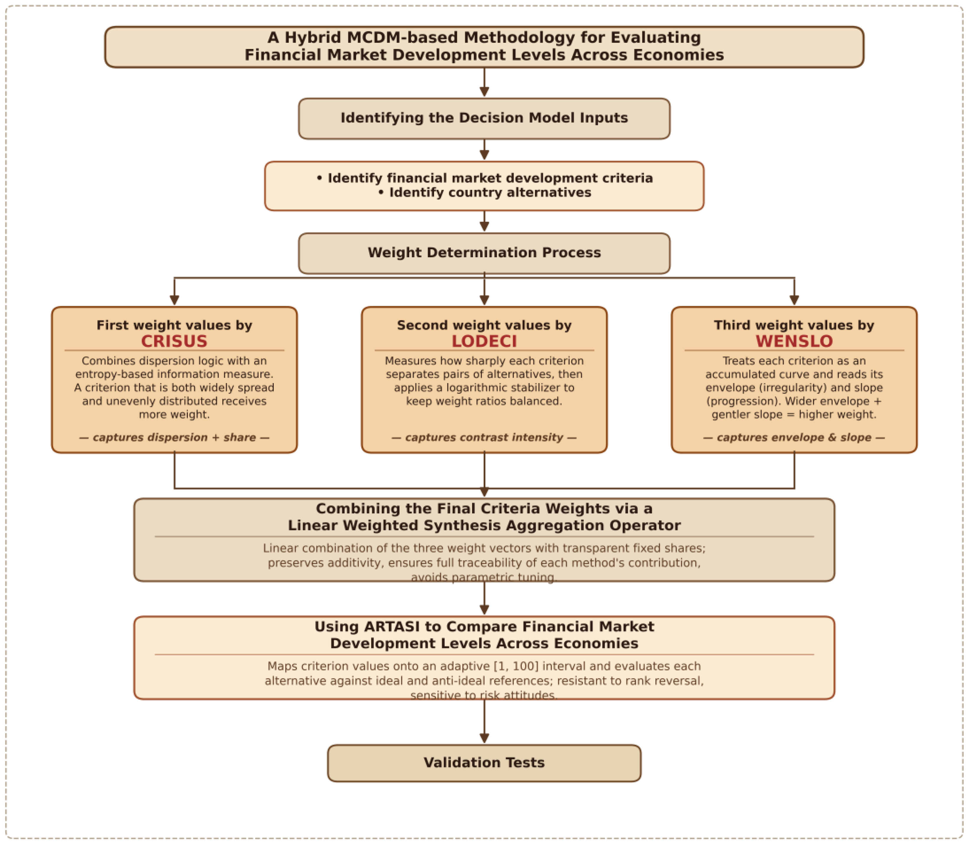
This section outlines the methodological foundations of the proposed integrated MCDM framework. In the first stage, the CRISUS, LODECI, and WENSLO procedures are presented in detail, given that they are combined to derive objective criterion weights. In the second stage, the ARTASI method is introduced step by step as the ranking tool used to assess the relative financial market development levels of the selected economies. The overall flow of the introduced hybrid methodology is illustrated in Figure 1.

3.1. Estimating the First Vector of Criterion Weights Employing the CRISUS Methodology

The CRISUS technique, introduced by Adalar and Işık [27] is a recently developed objective criterion-weighting approach in the MCDM literature. It identifies which criteria are most informative for distinguishing among decision alternatives by combining two intuitive ideas: the wider the values of a criterion are spread, and the more unevenly they are distributed within that criterion, the more discriminatory information it carries. To capture this, this algorithm first normalizes the decision matrix in two stages, and then combines the sum of squares of each criterion’s normalized values with its standard deviation to produce the final weight. This methodology thereby integrates statistical dispersion logic with the information-theoretic foundation of entropy in a single computational step. The computational procedure of this procedure is delineated as follows:

Step 1. Forming an initial performance matrix. This matrix, shown in Equation (1), includes m alternatives $A_p$ ($p=1, 2, \dots , m$) and n criteria $C_q$ ($q=1, 2, \dots , n$).

$$Y={\left[y_{pq}\right]}_{mxn}$$

(1)

Here, $y_{pq}$ indicates the observed performance value of alternative $A_p$, with respect to criterion $C_q$.

Step 2. Obtaining the first normalized decision matrix. In this step, vector normalization is employed to standardize the elements of the initial decision matrix. In this context, benefit-type and cost-type criteria are transformed in accordance with Equations (2) and (3), respectively.

$$f_{pq}={\displaystyle \frac{y_{pq}}{\sqrt{{\displaystyle {\displaystyle {\sum }_{p=1}^m}}{y}_{pq}^2}}},\forall q\in B$$

(2)

$$f_{pq}=1-{\displaystyle \frac{y_{pq}}{\sqrt{{\displaystyle {\displaystyle {\sum }_{p=1}^m}}{y}_{pq}^2}}},\forall q\in NB$$

(3)

Here, $B$ refers to the set of benefit-type criteria and $NB$ denotes the set of non-beneficial criteria.

Step 3. Constructing the second normalized decision matrix. The first-stage normalized values are further transformed to obtain a relative distribution matrix within the unit interval [0, 1]. For this purpose, Equation (4) is employed.

$$s_{pq}={\displaystyle \frac{f_{pq}}{{\displaystyle {\displaystyle {\sum }_{p=1}^m}}{f}_{pq}}}$$

(4)

Step 4. Computing the sum of squares for each criterion. Based on the second-stage normalized matrix, the concentration intensity of each criterion is quantified via a quadratic aggregation operator, as specified in Equation (5).

$${\rho }_q={\displaystyle {\displaystyle \sum _{p=1}^m}}{s}_{pq}^2$$

(5)

Step 5. Computing the standard deviation for each criterion. Employing the first-stage normalized matrix, the variability associated with each criterion is quantified by computing its standard deviation. The corresponding formulation is given as:

$${\sigma }_q=\sqrt{{\displaystyle \frac{{\displaystyle {\displaystyle {\sum }_{p=1}^m}}{\left(f_{pq}-{\overline{f}}_q\right)}^2}{m}}}$$

(6)

Here, ${\overline{f}}_q$ represents the mean value of the normalized performances under the criterion $C_q$.

Step 6. Deriving the first set of objective weights for the criteria.

$$w_q^{CRI}={\displaystyle \frac{{\rho }_q{\sigma }_q}{{\displaystyle {\displaystyle {\sum }_{q=1}^n}}{\rho }_q{\sigma }_q}}$$

(7)

3.2. Deriving the Second Objective Weight Vector via the LODECI Algorithm

The LODECI technique was introduced by Pala [28] as an objective weighting approach. The core idea behind LODECI is easy. A criterion is more important when it produces sharper differences among decision alternatives. Rather than gauging overall dispersion, this approach determines, for each decision alternative, the maximum gap that separates it from its most distant counterpart on the same criterion, and then aggregates these maximum separations across all decision alternatives. A logarithmic transformation is finally applied so that no single criterion dominates the weight vector, ensuring a balanced and decision-maker-acceptable distribution of importance. The computational steps of this technique are summarized as follows:

Step 1. Form the initial decision matrix presented in Equation (1).

Step 2. Normalizing the performance matrix. The elements of the initial decision matrix are normalized by employing a max-based normalization procedure. During this process, Equation (8) is applied to benefit-type criteria, whereas Equation (9) is utilized for non-beneficial (cost-type) criteria.

$$l_{pq}={\displaystyle \frac{y_{pq}}{max\left\{y_{pq}|1\le p\le m\right\}}},\forall q\in B$$

(8)

$$l_{pq}={\displaystyle \frac{min\left\{y_{pq}|1\le p\le m\right\}}{y_{pq}}}, \forall q\in NB$$

(9)

Step 3. Deriving the decomposition intensity of alternatives. The decomposition value captures the maximum structural deviation of each alternative from all other alternatives under a given criterion, thereby reflecting the contrast intensity inherent in that criterion. In this manner, the extreme discriminatory capability of each criterion is quantified at the alternative level. Accordingly, for each alternative $A_p$ evaluated under criterion $C_q$, the decomposition value is defined as:

$${DV}_{pq}=\underset{r\ne p}{m\mathrm{a}\mathrm{x}}\left\{\left|l_{pq}-l_{rq}\right|\right\},p=1, 2, \dots m;q=1, 2, \dots n$$

(10)

Here, while $l_{pq}$ denotes the normalized performance value of the alternative $A_p$ under criterion $C_q$, and $r$ represents the index of competing alternatives $(r=1, 2, \dots ,m;r\ne p)$.

Step 4. Obtaining the logarithmic decomposition value of each criterion. The logarithmic decomposition value of the criterion $C_q$ is computed with the aid of Equation (11).

$${LDV}_q=ln\left(1+{\displaystyle \frac{1}{m}}{\displaystyle {\displaystyle \sum _{p=1}^m}}{DV}_{pq}\right), q=1, 2, \dots n$$

(11)

Step 5. Deriving the second set of objective weights for the criteria. Following the computation of the logarithmic decomposition values, the final objective weights of the criteria are obtained through normalization. Specifically, the weight assigned to the criterion $C_q$ is calculated as:

$$w_q^{LOD}={\displaystyle \frac{{LDV}_q}{{\displaystyle {\displaystyle {\sum }_{q=1}^n}}{LDV}_q}}$$

(12)

3.3. Computing the Third Objective Weighting Vector Through the WENSLO Approach

The WENSLO approach, introduced by Pamucar et al. [29], is one of the recently developed objective weighting approaches. WENSLO gauges how much information each criterion carries by looking at the shape of its values. This technique first lines up the normalized values of a criterion and adds them up step by step. This produces a curve that gradually rises from 0 to 1. Two simple features of this curve are then examined—how wavy the curve is (its envelope) and how steeply it climbs (its slope). A criterion whose curve is wavy but rises gently is treated as more informative, because it spreads its information across many alternatives. A criterion whose curve is smooth and rises steeply is treated as less informative, because its information is concentrated in only a few points. The computational procedure of this algorithm is outlined below.

Step 1. Formulating the initial decision matrix according to Equation (1).

Step 2. Normalization of the elements of the initial decision matrix. After constructing the initial performance matrix, its elements are normalized via a linear normalization approach as defined in Equation (13):

$$z_{pq}={\displaystyle \frac{y_{pq}}{{\displaystyle {\displaystyle {\sum }_{p=1}^m}}{y}_{pq}}}, q=1, 2, \dots , n$$

(13)

This transformation generates the normalized decision matrix ${Z=\left[z_{pq}\right]}_{m\times n}$. By definition, the normalized elements satisfy $0<z_{pq}<1$, and for each criterion $C_q$, the summation of normalized values across all alternatives equals unity, i.e., ${\displaystyle {\displaystyle {\sum }_{p=1}^m}}{z}_{pq}=1$.

Step 3. Finding the criterion class interval. Following a Sturges-type formulation, the magnitude of the class interval for each criterion is identified in order to quantify the dispersion range of the normalized values. For the q-th criterion, the class interval $∆z_q$ is computed according to Equation (14):

$$∆z_q={\displaystyle \frac{max\left\{z_{pq}|p=1, 2, \dots , m\right\}-min\left\{z_{pq}|p=1, 2, \dots , m\right\}}{1+3.322\times \mathrm{l}\mathrm{o}\mathrm{g}\left(m\right)}}, q=1, 2, \dots , n$$

(14)

Step 4. Calculation of the criterion envelope. This step is grounded in the geometric concept of Euclidean distance in a two-dimensional space. The envelope measure reflects the cumulative structural variation of each criterion by aggregating the distances between successive normalized values along the criterion dimension. For the q-th criterion, the envelope $E_q$ is computed as:

$$E_q={\displaystyle {\displaystyle \sum _{p=1}^{m-1}}}\sqrt{{\left(z_{(p+1)q}-z_{pq}\right)}^2+{\left(∆z_q\right)}^2}, q=1, 2, \dots , n$$

(15)

Step 5. Computation of the criterion slope. The slope associated with each criterion is determined to quantify the inclination of the normalized distribution. For the q-th criterion, the slope ${tan\phi }_q$ is calculated as:

$${tan\phi }_q={\displaystyle \frac{{\displaystyle {\displaystyle {\sum }_{p=1}^m}}{z}_{pq}}{(m-1)∆z_q}}, q=1, 2, \dots , n$$

(16)

Step 6. Obtaining the envelope–slope ratio. The envelope–slope ratio integrates the dispersion magnitude, represented by the envelope, and the distribution inclination, represented by the slope, into a single structural indicator. This unified measure reflects the relative informational contribution of each criterion within the decision framework. For the q-th criterion, the envelope–slope ratio is defined as:

$${\theta }_q={\displaystyle \frac{E_q}{{tan\phi }_q}}, q=1, 2, \dots , n$$

(17)

Step 7. Deriving the final criterion weights. The final objective weights are obtained by normalizing the envelope–slope ratios. The weight associated with the q-th criterion is calculated as:

$$w_q^{WEN}={\displaystyle \frac{{\theta }_q}{{\displaystyle {\displaystyle {\sum }_{q=1}^n}}{\theta }_q}}, q=1, 2, \dots , n$$

(18)

3.4. Formulating a Composite Data-Driven Weighting Structure via Linear Integration

In MCDM models, the specification of criterion weights directly influences the stability and consistency of the final ranking outcomes. Distinct objective weighting procedures emphasize different structural properties of the decision matrix—such as dispersion, contrast intensity, and distributional geometry—which generally yield divergent weight vectors. These differences originate from the underlying mathematical formulation of each method and its associated normalization approach, since the latter is not an interchangeable preprocessing step but an integral component of the procedure’s analytical foundation. CRISUS adopts vector normalization (Equations (2) and (3)) because its quadratic concentration operator (Equation (5)) requires unit-length scaling for cross-criterion comparability of squared deviations. LODECI applies max-based normalization (Equations (8) and (9)) because its decomposition value (Equation (10)), defined as the maximum pairwise deviation among alternatives, is meaningful only when each criterion is rescaled relative to its own maximum. WENSLO employs sum-based normalization (Equation (13)) because the envelope–slope formulation (Equation (14)–(17)) requires that normalized values across alternatives sum to unity for the geometric construction to be well-defined. Imposing a uniform normalization rule would therefore violate the analytical premises of each procedure and compromise the structural properties they are designed to capture; preserving each method’s native normalization is consequently a methodological requirement rather than a stylistic preference. To attenuate the procedure-specific biases that arise from these distinct analytical perspectives and to derive a composite weight vector that is robust to any single procedure’s idiosyncratic assumptions, the three weight vectors are aggregated through the linear integration scheme defined in Equation (19):

$$w_q^{INT}=\xi w_q^{CRI}+\eta w_q^{LOD}+\left(1-\left(\xi +\eta \right)\right)w_q^{WEN}$$

(19)

Here, $w_q^{CRI}$, $w_q^{LOD}$, and $w_q^{WEN}$ denote the weight values of the criterion $C_q$ obtained from CRISUS, LODECI, and WENSLO, respectively. The parameters $\xi$ and $\eta$ $\left(\in [0, 1]\right)$ control the proportional influence of the three objective weight vectors within the linear integration framework. For the baseline scenario, equal contribution coefficients ($\xi$ = $\eta$ = 1/3) are adopted. The theoretical justification for both the linear aggregation form and the equal-weight baseline is developed in Section 3.7.

3.5. Constructing the Comparative Ranking of Alternatives Under the ARTASI Framework

ARTASI is a recently developed MCDM approach introduced by Pamucar et al. [30]. The defining feature of ARTASI lies in its standardization logic. Conventional ranking methods compress all criterion values into the [0, 1] interval, which tends to cluster alternatives and obscure small but meaningful differences between them. ARTASI instead maps each criterion onto a wider, adaptively chosen scale—for instance, [1, 100]—and assesses every alternative against both an ideal and an anti-ideal reference point, combining the two resulting utility values into a single ranking score. This adaptive standardization preserves the original distribution of the data, strengthens the discriminatory power of the final ordering, and makes the method structurally resistant to the rank-reversal problem. The computational steps of the ARTASI are outlined below.

Step 1. Creating the initial decision matrix based on Equation (1).

Step 2. Identifying the absolute minimum and maximum values. Following the construction of the initial performance matrix in Equation (1), the absolute lower and upper reference limits of the q-th criterion are computed in accordance with Equations (20) and (21), respectively.

$$y_q^{max}=max\left\{y_{pq}|p=1, 2, \dots , m\right\}+{max\left\{y_{pq}|p=1, 2, \dots , m\right\}}^{1/m}$$

(20)

$$y_q^{min}=min\left\{y_{pq}|p=1, 2, \dots , m\right\}-{min\left\{y_{pq}|p=1, 2, \dots , m\right\}}^{{\displaystyle \frac{1}{m}}}$$

(21)

Step 3. Standardizing the initial decision matrix elements. The criteria forming the initial performance matrix may be either benefit- or cost-oriented and may also be expressed in heterogeneous measurement units. To ensure comparability across criteria, all performance values are mapped into a common standardized interval. Conventional normalization techniques typically transform matrix elements into the interval [0, 1]. However, such a restricted range may lead to value compression and reduce dispersion sensitivity, particularly when the number of alternatives is relatively large. To mitigate this limitation, ARTASI allows the bounds of the standardized interval to be predefined by the decision-makers. In the current analysis, the elements of the performance matrix are mapped into the interval [1, 100]. Accordingly, each element $y_{pq}$ is standardized as:

$${\phi }_{pq}={\displaystyle \frac{(100-1)y_{pq}+y_q^{max}-100y_q^{min}}{y_q^{max}-y_q^{min}}}$$

(22)

Here, 100 and 1 denote the upper and lower bounds of the standardized interval, respectively. The terms $y_q^{max}$ and $y_q^{min}$ stand for the absolute maximum and minimum values of the criterion $C_q$, computed in Step 2. However, if there is a cost-oriented criterion in the performance matrix, it is modified by implementing the reverse sorting procedure shown in Equation (23).

$${\psi }_{pq}=max\left\{{\phi }_{pq}|p=1, 2, \dots , m\right\}+min\left\{{\phi }_{pq}|p=1, 2, \dots , m\right\}-{\phi }_{pq}$$

(23)

Furthermore, if the criterion in the decision matrix is benefit-oriented, then ${\psi }_{pq}$ is assumed to be equal to ${\phi }_{pq}$. In this way, the final standardized initial performance matrix $\varphi ={({\psi }_{pq})}_{m\times n}$ is produced.

Step 4. Determining the utility degrees with respect to the ideal and anti-ideal references. The usefulness degree of alternative $A_p$ under criterion $C_q$ with respect to the ideal value is computed using Equation (24).

$${\omega }_{pq}^{+}=100{\displaystyle \frac{{\psi }_{pq}}{max\left\{{\psi }_{pq}|p=1, 2, \dots , m\right\}}}{w}_q^{INT}$$

(24)

Here, ${\psi }_{pq}$ denotes the standardized performance value obtained in Step 3, and $w_q^{INT}$ is the integrated criterion weight defined in Equation (19).

For the anti-ideal reference, an inverse proportional utility component is first derived as:

$${\omega }_{pq}=100{\displaystyle \frac{min\left\{{\psi }_{pq}|p=1, 2, \dots , m\right\}}{{\psi }_{pq}}}{w}_q^{INT}$$

(25)

Since Equation (25) yields an inverse utility structure (i.e., lower values of ${\psi }_{pq}$ produce larger ${\omega }_{pq}$), it is subsequently re-scaled through Equation (26) to obtain the anti-ideal usefulness degree.

$${\omega }_{pq}^{-}=max\left\{{\omega }_{pq}|p=1, 2, \dots , m\right\}+min\left\{{\omega }_{pq}|p=1, 2, \dots , m\right\}-{\omega }_{pq}$$

(26)

Step 5. Aggregating the utility degrees of alternatives. Following the computation of ${\omega }_{pq}^{+}$ and ${\omega }_{pq}^{-}$ in Step 4, the aggregated utility degrees of the alternative $A_p$ under the ideal and anti-ideal references are computed according to Equations (27) and (28), respectively.

$${\varsigma }_p^{+}={\displaystyle {\displaystyle {\sum }_{q=1}^n}}{\omega }_{pq}^{+}$$

(27)

$${\varsigma }_p^{-}={\displaystyle {\displaystyle {\sum }_{q=1}^n}}{\omega }_{pq}^{-}$$

(28)

Step 6. Deriving the final utility function and the alternatives’ rankings. The overall performance of each alternative is determined through a parametric aggregation structure. The final utility function of the alternative $A_p$ is defined as:

$${\sigma }_p=\left({\varsigma }_p^{+}+{\varsigma }_p^{-}\right){\left[\epsilon {\left(f\left({\varsigma }_p^{+}\right)\right)}^{\beta }+\left(1-\epsilon \right){\left(f\left({\varsigma }_p^{-}\right)\right)}^{\beta }\right]}^{{\displaystyle \frac{1}{\beta }}}$$

(29)

Here, $\epsilon \in [0, 1]$, $\beta \ge 1$, $f\left({\varsigma }_p^{+}\right)={\displaystyle \frac{{\varsigma }_p^{+}}{{\varsigma }_p^{+}+{\varsigma }_p^{-}}}$, and $f\left({\varsigma }_p^{-}\right)={\displaystyle \frac{{\varsigma }_p^{-}}{{\varsigma }_p^{+}+{\varsigma }_p^{-}}}$

If $\epsilon$ and $\beta$ parameters are taken as $\epsilon =0.5$ and $\beta$ = 1, the final utility functions can be computed more easily. Thus, we can transform the final utility functions into the following equation:

$${\sigma }_p=({\varsigma }_p^{+}+{\varsigma }_p^{-}){\displaystyle \frac{f\left({\varsigma }_p^{+}\right)+f\left({\varsigma }_p^{-}\right)}{2}}$$

(30)

Lastly, the alternatives’ priority order is obtained from the final utility functions, where the alternative with the highest ${\sigma }_p$ value is chosen as the best option.

3.6. Rationale for the Selection of CRISUS, LODECI, WENSLO, and ARTASI

The selection of the four algorithms that constitute the hybrid MCDM approach suggested in this manuscript is based on a comparative methodological assessment rather than arbitrary preference. Each technique was chosen because it addresses a different structural limitation observed in commonly used MCDM instruments. This subsection explains the comparative rationale behind each selection.

3.6.1. Rationale for CRISUS

CRISUS method builds upon the theoretical foundations of both the Statistical Variance (SV) and Entropy approaches, but eliminates their respective shortcomings. As mathematically demonstrated by Adalar and Işık [27], the Entropy technique utilizes a fixed Boltzmann-type constant k = 1/ln(m) uniformly across all criteria, which oversimplifies the measurement of uncertainty when criteria differ in their dispersion characteristics. The SV approach, conversely, relies on a single deviation operator that becomes unstable as the number of alternatives grows. CRISUS overcomes both limitations through a two-stage normalization procedure combined with a sum-of-squares operator, allowing the variability of each criterion to be captured while avoiding the inconsistency inherent in subjective methods such as AHP or BWM, which suffer from expert-induced inconsistency when the criterion set is large. Comparative experiments reported by Adalar and Işık [27] demonstrate that CRISUS exhibits high consistency with established objective weighting methods, with Pearson correlation coefficients above 0.8414 across all nine benchmark techniques tested (the lowest being 0.84 with MEREC and the highest 0.9987 with MAXC), indicating that CRISUS captures the underlying weight structure reliably while offering greater computational simplicity.

3.6.2. Rationale for LODECI

The LODECI algorithm was selected because it explicitly resolves a long-standing contradiction between Entropy and MEREC. These two widely utilized algorithms operate at opposite extremes of the contrast-intensity spectrum, and Ecer and Pamucar [35] have shown that both tend to produce excessively skewed weight ratios that decision-makers find unacceptable in practice. LODECI integrates both perspectives via a maximum-decomposition logic combined with a logarithmic stabilization function, producing balanced weight intervals. As empirically demonstrated by Pala [28] across four illustrative samples with three to six criteria, the maximum–minimum weight range of LODECI remained between 0.0009 and 0.2353, whereas the corresponding ranges of MEREC (0.2240–0.4100) and Entropy (0.5729–0.6280) were substantially wider, indicating that both algorithm produce excessively skewed weight distributions. This stabilization property is particularly valuable in the present application, where the criterion set captures diverse institutional, legal, market-based, and macro-financial dimensions of financial market development.

3.6.3. Rationale for WENSLO

WENSLO’s weighting approach is preferred over conventional procedures such as Entropy, CRITIC, and Standard Deviation (SD) for three principal reasons. First, unlike methods that require separate normalization formulas for benefit-type and cost-type criteria, the WENSLO normalization procedure is independent of criterion type, which eliminates a documented source of inconsistency in traditional objective weighting and ensures that the calculation process is unaffected by criteria preferences [29]. Second, WENSLO captures the underlying behavior of each criterion as a quasi-time-series sequence via an accumulation procedure rooted in Grey System theory; this enables the extraction of the governing tendency of each criterion regardless of its randomness or volatility. Third, validation experiments reported by Pamucar et al. [29] demonstrate Spearman correlation coefficients of 0.991 with Entropy, 0.976 with CRITIC, and 0.967 with SD, confirming that WENSLO produces weight distributions consistent with established methods while offering low computation time, good transparency, and reduced mathematical complexity for end-users.

3.6.4. Rationale for ARTASI

ARTASI was preferred in the ranking of country alternatives because it offers structural advantages over commonly used tools such as WASPAS, TOPSIS, MABAC, and MARCOS. Unlike these four algorithms, ARTASI maps the criterion values to adaptively defined standardized ranges, whose lower and upper bounds can be chosen according to the characteristics of the decision problem, instead of limiting the criterion values to a fixed [0, 1] normalization range using additive (WASPAS), vector-based (TOPSIS), maximum-minimum (MABAC), linear (MARCOS) procedures. This adaptive standardization preserves the original disposition of the data and produces a more discriminative ranking, which is particularly valuable when 16 closely ranked African economies must be distinguished. It further incorporates a dedicated reverse-sorting algorithm for cost-type criteria that protects the original information distribution, and its utility-based aggregation function includes two stabilization parameters that allow the simulation of different risk attitudes and dynamic decision environments. Equally important, the standardization function makes ARTASI structurally resistant to the rank-reversal problem documented in the other four algorithms, and its adaptive interval mechanism provides a high degree of generalization across decision problems of varying scale [30,36].

3.7. Rationale for the Introduced Weight Aggregation Strategy

While CRISUS, LODECI, and WENSLO can each independently generate criterion weights, the introduced weight-combining strategy integrates them jointly because objective weighting techniques rest on heterogeneous theoretical foundations and systematically produce different weight structures for the same dataset [28,35,37]. Relying on a single weighting strategy embeds the assumptions of that procedure into the analysis, whereas combining three structurally distinct tools carries out a methodological triangulation that neutralizes such biases, provides built-in cross-validation, and produces a weight vector that remains stable under perturbations of the data or criteria set. This feature is particularly important in cross-country comparative environments where datasets are periodically revised.

The aggregation utilizes a linear operator on theoretical rather than purely operational grounds. Linear integration preserves the simplex structure of the input weight vectors and the additive scale on which CRISUS, LODECI, and WENSLO each define their criterion contributions, so that the composite vector remains a valid normalized weight without the introduction of additional parametric assumptions. This treatment is consistent with established practice for combining heterogeneous objective weighting procedures in MCDM, where method-specific biases are best neutralized through methodological triangulation rather than through reliance on a single tool [37,38]. Non-linear alternatives—geometric averaging or rank-based pooling—either violate this preserving property or introduce calibration parameters that reintroduce analyst-induced subjectivity, contradicting the objective character of the weighting stage. 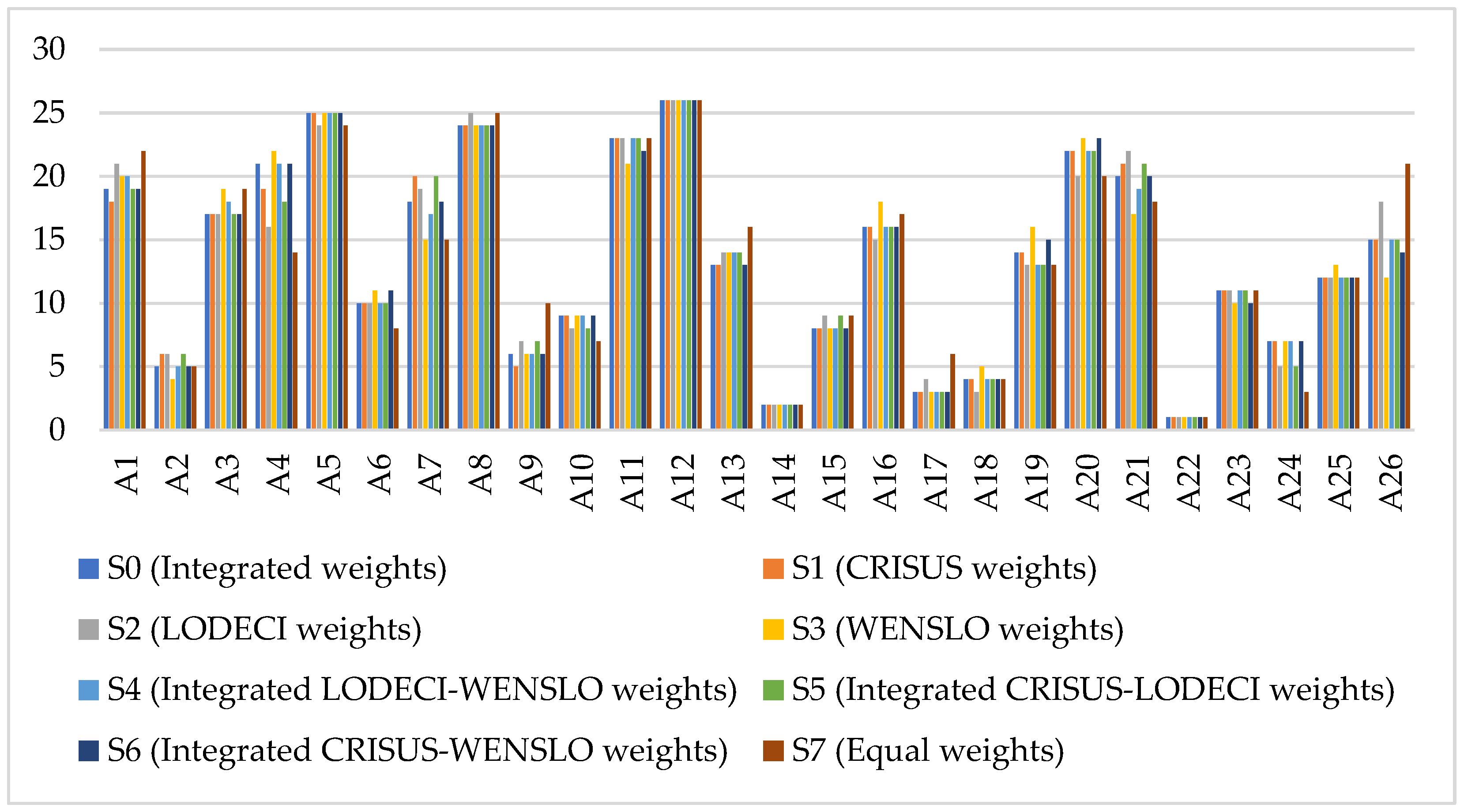The equal-coefficient baseline ($\xi$ =$\eta$ = 1/3) follows from the same logic. In the absence of empirical evidence that any one of the three procedures dominates the others in recovering the latent criterion-importance structure, equal allocation is the only weighting that does not impose an unjustified preference among them, thereby preserving the fully data-driven character of the framework. 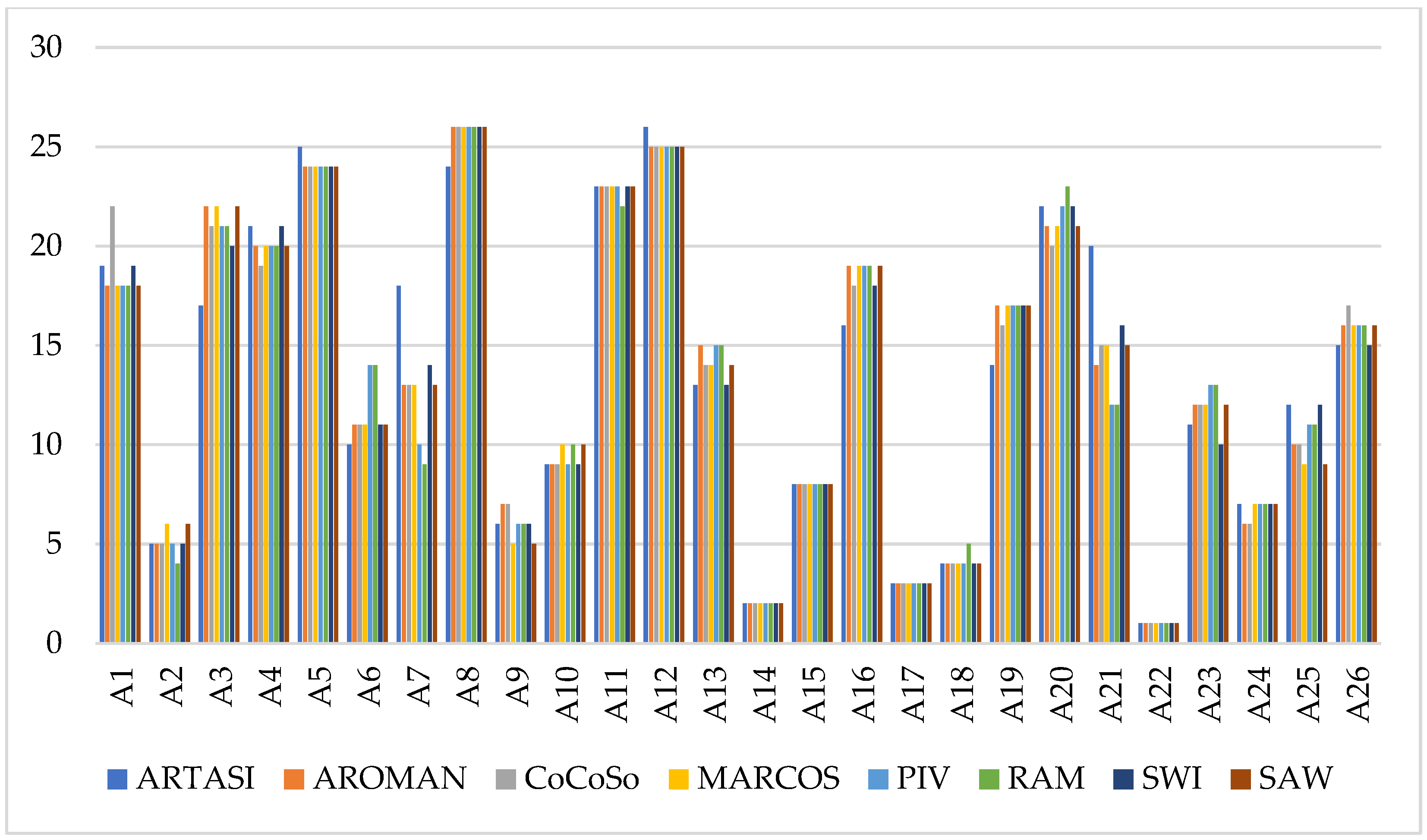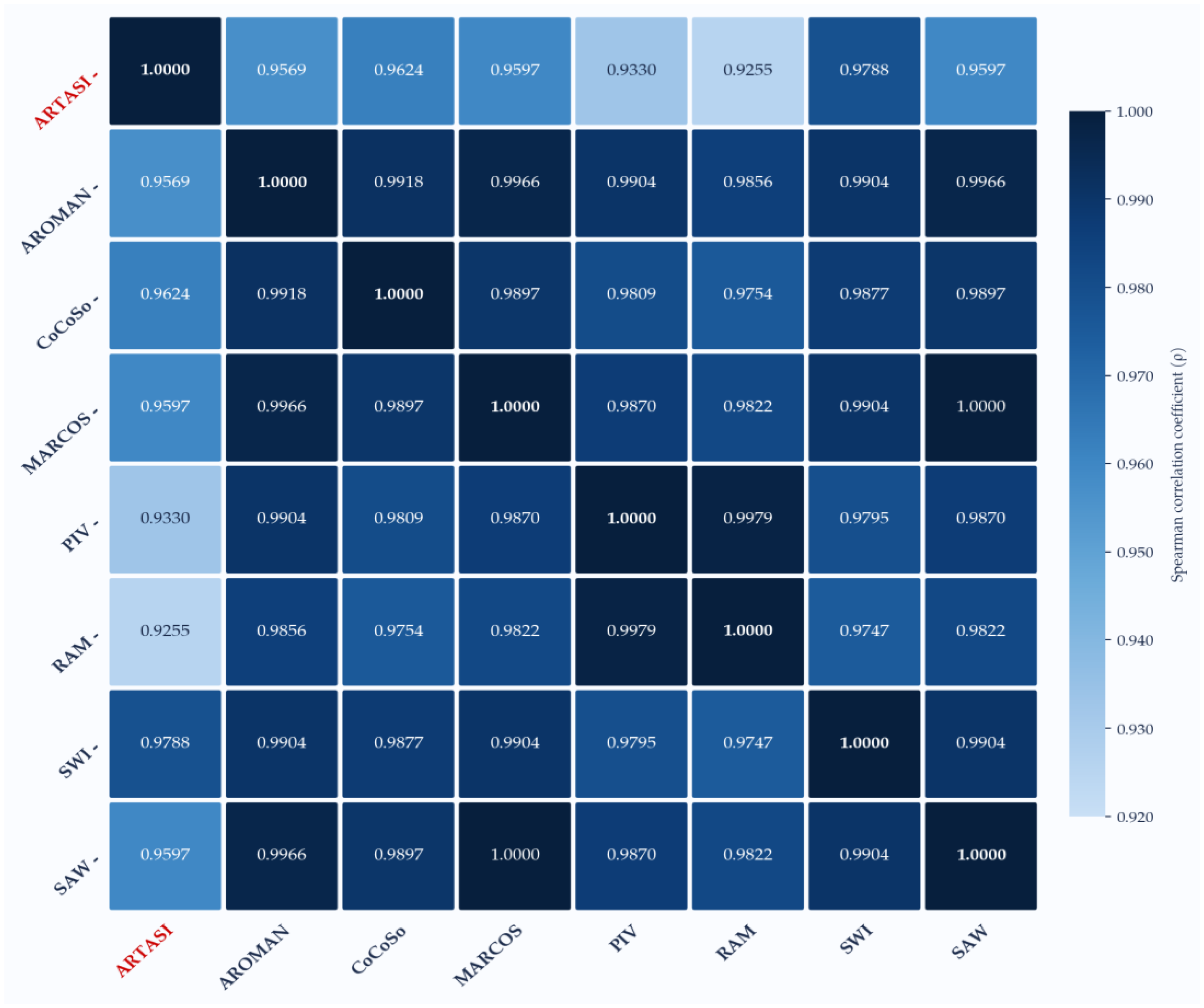Equal weighting is therefore a principled choice rather than a default-by-omission, and its empirical robustness is confirmed by the sensitivity analysis in Section 5.1 and by the comparative MCDM benchmarking presented in Section 5.2.

Two further considerations justify the exclusive reliance on objective methods rather than the subjective–objective hybridization frequently advocated in the MCDM literature. First, the assessment criteria adopted in the existing manuscript originate from a publicly disclosed and standardized index, which already encodes substantial expert judgment at the indicator-construction stage. Reintroducing subjective weights at the aggregation stage would therefore double-count expert input and compromise reproducibility. Second, subjective procedures such as AHP and BWM are known to suffer from cognitive overload when the criteria set exceeds approximately seven elements and from inconsistency among experts with heterogeneous backgrounds, both problematic in the present cross-country institutional context. The introduced objective triangulation, therefore, produces fully reproducible weights from the data itself while preserving the analytical balance that hybrid models seek to achieve.

3.8. Procedural Summary of the Integrated Methodology

To facilitate readability and to consolidate the steps presented in Section 3.1, Section 3.2, Section 3.3, Section 3.4 and Section 3.5 into a single reference point, the complete computational flow of the introduced CRISUS-LODECI-WENSLO-ARTASI hybrid framework is summarized in Algorithm 1.

Algorithm 1. The CRISUS-LODECI-WENSLO-ARTASI hybrid procedure.

Input: Initial decision matrix $Y={\left[y_{pq}\right]}_{mxn}$ with $m$ alternatives and $n$ criteria; criterion-type vector (benefit/cost); integration parameters $\xi$, $\eta$ ∈ [0, 1]; ARTASI parameters $\epsilon$, $\beta$. Output: Final ranking of alternatives based on ${\sigma }_p$

Stage I—Objective criterion weighting Step 1. Apply the CRISUS procedure to $Y$: construct the two-stage normalized matrix via vector normalization (Equations (2) and (3)) followed by relative-share normalization (Equation (4)); compute the sum-of-squares concentration intensity (Equation (5)) and the standard deviation (Equation (6)) for each criterion; then derive the first weight vector $w_q^{CRI}$ as the normalized product of these two operators (Equation (7)). Step 2. Apply the LODECI procedure to $Y$: apply max-based normalization (Equations (8) and (9)); for each alternative, compute the decomposition value as its maximum pairwise deviation under each criterion (Equation (10)); aggregate these values through a logarithmic transformation (Equation (11)); and derive the second weight vector $w_q^{LOD}$ by normalizing the logarithmic decomposition values (Equation (12)). Step 3. Apply the WENSLO procedure to $Y$: apply linear normalization (Equation (13)); compute the class interval (Equation (14)), the envelope (Equation (15)), and the slope (Equation (16)) of each criterion; obtain the envelope–slope ratio (Equation (17)); and derive the third weight vector $w_q^{WEN}$ by normalizing these ratios (Equation (18)).

Stage II—Linear integration of the three weight vectors Step 4. Combine $w_q^{CRI}$, $w_q^{LOD}$, and $w_q^{WEN}$ through the linear integration operator with weights $\xi$, $\eta$, and (1 − $\xi$ − $\eta$) to obtain the integrated criterion weight vector $w_q^{INT}$ (Equation (19)). Under the baseline scenario, $\xi$ = $\eta$ = 1/3.

Stage III—Adaptive ranking of alternatives via ARTASI Step 5. From the original matrix $Y$, determine the absolute lower and upper reference bounds $y_q^{max}$, $y_q^{min}$ for each criterion via Equations (20) and (21). Step 6. Standardize Y onto the adaptive interval [1, 100] using Equation (22); for cost-type criteria, additionally apply the reverse-sorting transformation in Equation (23). The output is the standardized matrix $\varphi ={\left({\psi }_{pq}\right)}_{m\times n}$ Step 7. Using $\varphi$ and the integrated weights $w_q^{INT}$ from Step 4, compute the ideal-reference utility ${\omega }_{pq}^{+}$ via Equation (24) and the anti-ideal-reference utility ${\omega }_{pq}^{-}$ via Equations (25) and (26). Step 8. Aggregate the criterion-level utilities into alternative-level utility scores ${\varsigma }_p^{+}$ and ${\varsigma }_p^{-}$ via Equations (27) and (28). Step 9. Compute the final utility score ${\sigma }_p$ of each alternative through the parametric aggregation in Equation (29)—or, under the baseline parameterization $\epsilon$ = 0.5, $\beta$ = 1, through the simplified form in Equation (30). Rank alternatives in descending order of ${\sigma }_p$.

4. Case Study: Comparative Assessment of Financial Market Development in Africa

This section operationalizes the CRISUS-LODECI-WENSLO-ARTASI hybrid methodology on a structured real-world dataset covering financial market development across selected African economies. The decision matrix is constructed from four consecutive annual editions (2022–2025) of the Absa Africa Financial Markets Index (AFMI), published jointly by the Official Monetary and Financial Institutions Forum (OMFIF) and Absa Group Limited and issued annually since 2017 as a standardized, methodologically consistent benchmark of market openness, infrastructure, and institutional quality across the continent [39]. For each of the six AFMI pillars ($C_1-C_6$) and each of the twenty-six retained economies ($A_1-A_{26}$), the corresponding pillar-level scores were extracted from the official AFMI reports and the arithmetic mean over the four-year window was taken as the criterion value entering the decision matrix, ensuring that the empirical inputs reflect persistent structural characteristics rather than transitory shocks or cyclical fluctuations.

This section is organized into three analytically coherent sub-sections. The first sub-section introduces the evaluation criteria, which represent the core structural criteria of financial market development, and details their measurement foundations within the AFMI framework. The second sub-section defines the alternative economies included in the analysis. Finally, the third sub-section reports the empirical findings derived from the implementation of the WENSLO-LODECI-CRISUS-ARTASI hybrid algorithm, providing a comparative ranking and detailed analysis of the results.

4.1. Definition of Financial Market Development Criteria

Financial market development is operationalized through the AFMI, an annual benchmark published by OMFIF and Absa Group with the support of the United Nations Economic Commission for Africa and the African Development Bank. The AFMI is preferred over established global frameworks—most notably the IMF Financial Development Index of Svirydzenka [7], which itself refines the 4 × 2 institutions-versus-markets architecture of Čihák et al. [10]—for two structural reasons. First, the AFMI is purpose-designed for African financial systems and incorporates indicators of institutional, legal, and macroeconomic context that the IMF index explicitly excludes [7]. Second, its six-pillar architecture spans the full set of dimensions identified in the law-and-finance literature reviewed by Beck and Levine [40]—investor protection, contract enforcement, and property rights—which Čihák et al. [10] classify as the enabling environment and consequently place outside their core measurement matrix. The criteria examined in the analysis are summarized below [39].

Market depth $\left(C_1\right)$: This criterion serves as a proxy for the size, liquidity, and sophistication of domestic equity and bond markets. It evaluates the capacity of a financial ecosystem to absorb large-scale transactions with minimal price volatility, primarily measured through domestic market capitalization as a percentage of GDP, trading turnover ratios, and the diversity of available financial instruments. Furthermore, it considers the efficiency of primary dealer systems and the availability of secondary market makers, which are essential for maintaining continuous price discovery and facilitating market clearing.

Access to foreign exchange $\left(C_2\right)$: This criterion reflects the degree of capital mobility and the efficiency of the foreign exchange market. It examines the adequacy of central bank reserves relative to import coverage and assesses FX liquidity through interbank turnover as a share of total merchandise trade. A critical component of this pillar is the evaluation of capital restrictions and the alignment of exchange rate regimes with international standards, such as the adoption of the FX Global Code, which ensures a transparent and predictable environment for international investors.

Market transparency, tax, and regulatory environment $\left(C_3\right)$: This indicator quantifies the quality of the institutional and regulatory framework governing financial activities. It encompasses the implementation of global prudential standards, such as the Basel Accords, and the adoption of International Financial Reporting Standards to mitigate information asymmetry. Additionally, it assesses the fiscal competitiveness of the market by analyzing withholding tax levels and the existence of double taxation treaties, while also considering modern regulatory trends such as Environmental, Social, and Governance reporting initiatives.

Pension fund development $\left(C_4\right)$: Recognizing the role of institutional investors in stabilizing capital markets, this criterion assesses the maturity and “domestic firepower” of the local pension industry. It measures the scale of pension fund assets relative to the working-age population and evaluates their capacity to provide long-term sustainable liquidity to domestically listed equities and bonds. A well-developed pension sector reduces reliance on volatile foreign capital and fosters the growth of deeper, more resilient financial markets.

Macroeconomic environment and transparency $\left(C_5\right)$: This indicator captures the fundamental economic stability that underpins financial market performance. It tracks key macroeconomic indicators, including GDP growth trajectories, inflation volatility, non-performing loan ratios, and external debt-to-GDP levels. Beyond static indicators, this pillar emphasizes “informational efficiency” by evaluating the frequency and reliability of macroeconomic data publication and the transparency of monetary policy decision-making processes.

Legal Standards and Enforceability $\left(C_6\right)$: It assesses the robustness of the legal infrastructure underpinning counterparty risk, in particular the enforceability of close-out netting and financial collateral arrangements, and alignment with the International Swaps and Derivatives Association (ISDA) and Global Master Repurchase Agreement (GMRA) master agreements.

Several of the underlying indicators aggregated into the AFMI pillars—most notably inflation volatility, non-performing-loan ratios, and external debt-to-GDP under Pillar 5, and effective withholding-tax rates under Pillar 3—are conceptually cost-type variables in standard economics. The AFMI rebases each underlying indicator onto a harmonized 10–100 scale at the construction stage, however, so that lower raw values of cost-type variables map to higher rebased pillar scores. Consequently, all six pillars enter the decision matrix as benefit-type criteria [39].

4.2. Definition of Alternative Countries

The empirical scope comprises twenty-six African economies retained from the twenty-nine countries appearing in the most recent AFMI edition [39]. The chosen alternatives and their analytical codes ($A_1-A_{26}$) are reported in

Table 2. Country alternatives.

Code	Country	Code	Country
$A_1$	Angola	$A_{14}$	Mauritius
$A_2$	Botswana	$A_{15}$	Morocco
$A_3$	Cameroon	$A_{16}$	Mozambique
$A_4$	Côte d’Ivoire	$A_{17}$	Namibia
$A_5$	DRC	$A_{18}$	Nigeria
$A_6$	Egypt	$A_{19}$	Rwanda
$A_7$	Eswatini	$A_{20}$	Senegal
$A_8$	Ethiopia	$A_{21}$	Seychelles
$A_9$	Ghana	$A_{22}$	South Africa
$A_{10}$	Kenya	$A_{23}$	Tanzania
$A_{11}$	Lesotho	$A_{24}$	Uganda
$A_{12}$	Madagascar	$A_{25}$	Zambia
$A_{13}$	Malawi	$A_{26}$	Zimbabwe

. Selection was based on the availability of complete observations on all six pillars across each annual edition of the 2022–2025 window. Three economies—Cabo Verde and Tunisia, which entered the AFMI roster in the 2023 edition, and Benin, which was added in the 2024 edition—were therefore excluded ex ante to safeguard the comparability and methodological consistency of the analysis.

The integrity of the input matrix warrants brief documentation. The empirical design implies an expected total of 26 × 6 × 4 = 624 country–criterion–year observations, and the assembled decision matrix is fully balanced: all 624 cells are populated by explicit numerical AFMI scores within the index’s harmonized [10, 100] range, with no occurrences of “n/a” or qualitative flags requiring substitution, so that the criterion values entering

Table 3. Initial decision-making matrix.

	${\mathit{C}}_1$	${\mathit{C}}_2$	${\mathit{C}}_3$	${\mathit{C}}_4$	${\mathit{C}}_5$	${\mathit{C}}_6$
${\mathit{A}}_1$	38.00	58.50	60.75	13.75	56.50	22.50
${\mathit{A}}_2$	56.00	66.50	75.25	59.25	86.00	27.50
${\mathit{A}}_3$	28.00	53.00	45.75	16.75	68.75	21.25
${\mathit{A}}_4$	33.25	56.00	53.75	12.25	72.50	22.50
${\mathit{A}}_5$	20.00	44.25	53.25	10.00	75.50	10.00
${\mathit{A}}_6$	47.25	78.50	85.00	18.00	77.00	32.50
${\mathit{A}}_7$	23.75	50.75	59.50	58.50	78.00	10.00
${\mathit{A}}_8$	10.00	43.50	41.75	11.00	65.00	13.75
${\mathit{A}}_9$	47.00	56.25	82.50	23.25	62.75	90.00
${\mathit{A}}_{10}$	39.25	71.50	88.00	19.75	75.25	55.00
${\mathit{A}}_{11}$	12.25	56.50	34.00	26.75	69.25	17.50
${\mathit{A}}_{12}$	16.50	71.50	33.50	10.00	64.25	10.00
${\mathit{A}}_{13}$	28.50	43.50	61.25	13.25	61.00	68.75
${\mathit{A}}_{14}$	58.25	76.25	92.75	59.75	74.00	97.50
${\mathit{A}}_{15}$	61.00	70.75	85.00	34.00	70.75	25.00
${\mathit{A}}_{16}$	34.00	49.00	45.25	15.75	70.00	26.25
${\mathit{A}}_{17}$	43.00	56.00	63.25	100.00	76.50	41.25
${\mathit{A}}_{18}$	55.50	63.00	86.25	24.50	75.50	92.50
${\mathit{A}}_{19}$	31.25	60.00	75.50	14.75	73.75	26.25
${\mathit{A}}_{20}$	34.75	55.25	50.50	11.50	68.75	22.50
${\mathit{A}}_{21}$	21.75	58.25	49.75	55.75	76.00	10.00
${\mathit{A}}_{22}$	99.50	88.25	94.50	65.25	78.25	100.00
${\mathit{A}}_{23}$	48.50	59.00	75.50	18.25	81.25	40.00
${\mathit{A}}_{24}$	45.75	72.00	76.75	17.25	85.00	87.50
${\mathit{A}}_{25}$	31.75	56.00	75.50	11.75	71.75	83.75
${\mathit{A}}_{26}$	17.75	36.50	79.75	22.50	69.00	40.00

reflect observed scores in their entirety, without imputation, interpolation, or smoothing at any stage [39]. The complete-case exclusion of Cabo Verde, Tunisia, and Benin was preferred over imputation for two reasons: AFMI pillar scores are aggregated composites of more than forty heterogeneous sub-indicators that pillar-level imputation cannot faithfully reconstruct, and the discriminative resolution of CRISUS, LODECI, and WENSLO depends directly on the empirical dispersion of the matrix, which imputation systematically compresses. The four AFMI editions share a single published methodology with stable pillar definitions, weights, and indicator coverage across 2022–2025; earlier editions are deliberately excluded from the dataset because the AFMI underwent substantive methodological revisions in its 2022 edition that affected both the composition of several pillars and the construction of the underlying indicators that populate them. The retained twenty-six economies nonetheless span the full empirical range of AFMI scores observed in the window—from its highest-scoring leaders to its lowest-scoring frontier systems—supporting the comparative-ranking objective of this research.

The decision matrix entries themselves were computed as the four-year arithmetic mean of the corresponding AFMI pillar scores. Three considerations motivate this design. First, the AFMI country roster has expanded materially since the inaugural edition—from 17 countries in 2017 to 20 in 2018–2019, 23 in 2020–2021, 26 in 2022, 28 in 2023, and 29 in 2024–2025—so that any single-year specification would force a trade-off between recency and a stable, balanced panel of alternatives. Period averaging over 2022–2025 retains a methodologically homogeneous set of twenty-six economies for which all six pillars are observed in every annual edition. Second, financial market development is widely characterized in the literature as a slowly evolving institutional construct whose informational content is best captured by its long-run central tendency; the arithmetic mean therefore acts as a noise-attenuation operator that isolates the structural signal from cyclical components such as commodity cycles, pandemic-period disruptions, and exchange-rate fluctuations. Third, four-year averaging dampens the influence of transient policy adjustments and isolated administrative reforms—sources of variation that affect annual scores without altering the persistent profile of each economy.

4.3. The WENSLO-LODECI-CRISUS-ARTASI Algorithm Implementation and Results

This subsection reports the empirical implementation of the introduced CRISUS-LODECI-WENSLO-ARTASI approach and presents the corresponding findings in a stepwise manner. First, the objective criterion weight values derived from the CRISUS, LODECI, and WENSLO procedures are reported separately. Next, these three objective weight vectors are combined via a linear integration procedure to obtain the final set of criterion weights utilized in the ranking stage. Finally, the ARTASI tool is applied to the decision matrix by using the aggregated weights, and the relative performance ranking of the selected African economies is obtained.

4.3.1. The CRISUS Results

The first objective weight vector was derived through the implementation of the CRISUS algorithm on the decision matrix prepared for the selected African economies. As noted in Section 4.2, each matrix element reflects the arithmetic mean of the corresponding financial market development criterion over the 2022–2025 period. In accordance with the methodological framework of the CRISUS tool introduced in Section 3, the initial decision matrix was formulated according to Equation (1) and is given in Table 3. Given that all criteria contained in the initial decision matrix are benefit-type, the first normalized performance matrix was generated by applying Equation (2) and is displayed in

Table 4. First normalized performance matrix.

	${\mathit{C}}_1$	${\mathit{C}}_2$	${\mathit{C}}_3$	${\mathit{C}}_4$	${\mathit{C}}_5$	${\mathit{C}}_6$
${\mathit{A}}_1$	0.1766	0.1887	0.1733	0.0739	0.1524	0.0849
${\mathit{A}}_2$	0.2603	0.2145	0.2147	0.3186	0.2319	0.1038
${\mathit{A}}_3$	0.1302	0.1709	0.1305	0.0901	0.1854	0.0802
${\mathit{A}}_4$	0.1546	0.1806	0.1533	0.0659	0.1955	0.0849
${\mathit{A}}_5$	0.0930	0.1427	0.1519	0.0538	0.2036	0.0378
${\mathit{A}}_6$	0.2196	0.2532	0.2425	0.0968	0.2077	0.1227
${\mathit{A}}_7$	0.1104	0.1637	0.1697	0.3146	0.2104	0.0378
${\mathit{A}}_8$	0.0465	0.1403	0.1191	0.0592	0.1753	0.0519
${\mathit{A}}_9$	0.2185	0.1814	0.2353	0.1250	0.1692	0.3398
${\mathit{A}}_{10}$	0.1825	0.2306	0.2510	0.1062	0.2029	0.2076
${\mathit{A}}_{11}$	0.0569	0.1822	0.0970	0.1438	0.1868	0.0661
${\mathit{A}}_{12}$	0.0767	0.2306	0.0956	0.0538	0.1733	0.0378
${\mathit{A}}_{13}$	0.1325	0.1403	0.1747	0.0712	0.1645	0.2595
${\mathit{A}}_{14}$	0.2708	0.2459	0.2646	0.3213	0.1996	0.3681
${\mathit{A}}_{15}$	0.2836	0.2282	0.2425	0.1828	0.1908	0.0944
${\mathit{A}}_{16}$	0.1581	0.1580	0.1291	0.0847	0.1888	0.0991
${\mathit{A}}_{17}$	0.1999	0.1806	0.1804	0.5377	0.2063	0.1557
${\mathit{A}}_{18}$	0.2580	0.2032	0.2460	0.1317	0.2036	0.3492
${\mathit{A}}_{19}$	0.1453	0.1935	0.2154	0.0793	0.1989	0.0991
${\mathit{A}}_{20}$	0.1615	0.1782	0.1441	0.0618	0.1854	0.0849
${\mathit{A}}_{21}$	0.1011	0.1879	0.1419	0.2998	0.2050	0.0378
${\mathit{A}}_{22}$	0.4625	0.2846	0.2696	0.3509	0.2110	0.3775
${\mathit{A}}_{23}$	0.2255	0.1903	0.2154	0.0981	0.2191	0.1510
${\mathit{A}}_{24}$	0.2127	0.2322	0.2189	0.0928	0.2292	0.3303
${\mathit{A}}_{25}$	0.1476	0.1806	0.2154	0.0632	0.1935	0.3162
${\mathit{A}}_{26}$	0.0825	0.1177	0.2275	0.1210	0.1861	0.1510

. In the next stage, Equation (4) was applied to derive the second normalized performance matrix, the results of which are reported in

Table 5. Second normalized performance matrix.

	${\mathit{C}}_1$	${\mathit{C}}_2$	${\mathit{C}}_3$	${\mathit{C}}_4$	${\mathit{C}}_5$	${\mathit{C}}_6$
${\mathit{A}}_1$	0.0387	0.0377	0.0352	0.0185	0.0300	0.0206
${\mathit{A}}_2$	0.0570	0.0429	0.0436	0.0797	0.0457	0.0251
${\mathit{A}}_3$	0.0285	0.0342	0.0265	0.0225	0.0365	0.0194
${\mathit{A}}_4$	0.0338	0.0361	0.0312	0.0165	0.0385	0.0206
${\mathit{A}}_5$	0.0204	0.0285	0.0309	0.0134	0.0401	0.0091
${\mathit{A}}_6$	0.0481	0.0506	0.0493	0.0242	0.0409	0.0297
${\mathit{A}}_7$	0.0242	0.0327	0.0345	0.0787	0.0414	0.0091
${\mathit{A}}_8$	0.0102	0.0281	0.0242	0.0148	0.0345	0.0126
${\mathit{A}}_9$	0.0478	0.0363	0.0478	0.0313	0.0333	0.0823
${\mathit{A}}_{10}$	0.0399	0.0461	0.0510	0.0266	0.0400	0.0503
${\mathit{A}}_{11}$	0.0125	0.0364	0.0197	0.0360	0.0368	0.0160
${\mathit{A}}_{12}$	0.0168	0.0461	0.0194	0.0134	0.0341	0.0091
${\mathit{A}}_{13}$	0.0290	0.0281	0.0355	0.0178	0.0324	0.0629
${\mathit{A}}_{14}$	0.0593	0.0492	0.0538	0.0804	0.0393	0.0891
${\mathit{A}}_{15}$	0.0621	0.0456	0.0493	0.0457	0.0376	0.0229
${\mathit{A}}_{16}$	0.0346	0.0316	0.0262	0.0212	0.0372	0.0240
${\mathit{A}}_{17}$	0.0438	0.0361	0.0367	0.1345	0.0406	0.0377
${\mathit{A}}_{18}$	0.0565	0.0406	0.0500	0.0330	0.0401	0.0846
${\mathit{A}}_{19}$	0.0318	0.0387	0.0438	0.0198	0.0392	0.0240
${\mathit{A}}_{20}$	0.0354	0.0356	0.0293	0.0155	0.0365	0.0206
${\mathit{A}}_{21}$	0.0221	0.0376	0.0288	0.0750	0.0404	0.0091
${\mathit{A}}_{22}$	0.1013	0.0569	0.0548	0.0878	0.0416	0.0914
${\mathit{A}}_{23}$	0.0494	0.0381	0.0438	0.0245	0.0432	0.0366
${\mathit{A}}_{24}$	0.0466	0.0464	0.0445	0.0232	0.0452	0.0800
${\mathit{A}}_{25}$	0.0323	0.0361	0.0438	0.0158	0.0381	0.0766
${\mathit{A}}_{26}$	0.0181	0.0235	0.0462	0.0303	0.0367	0.0366

. Finally, Equations (5)–(7) were utilized to compute the sum of squares (${\rho }_q$), standard deviations (${\sigma }_q$), and objective weight values ($w_q^{CRI}$), whose results are given in

Table 6. Results obtained from the CRISUS methodology.

	${\mathit{C}}_1$	${\mathit{C}}_2$	${\mathit{C}}_3$	${\mathit{C}}_4$	${\mathit{C}}_5$	${\mathit{C}}_6$
${\mathit{\rho }}_{\mathit{q}}$	0.0479	0.0400	0.0413	0.0626	0.0388	0.0587
${\mathit{\sigma }}_{\mathit{q}}$	0.0889	0.0391	0.0526	0.1241	0.0189	0.1173
${\mathit{w}}_{\mathit{q}}^{\mathit{C}\mathit{R}\mathit{I}}$	0.1823	0.0669	0.0930	0.3321	0.0313	0.2944

.

4.3.2. The LODECI Results

The second objective weight vector was derived through the implementation of the LODECI algorithm. In the first stage, the initial performance matrix indicated in Table 3 was normalized with the help of Equation (8), and the normalized values are given in

Table 7. Normalized performance matrix.

	${\mathit{C}}_1$	${\mathit{C}}_2$	${\mathit{C}}_3$	${\mathit{C}}_4$	${\mathit{C}}_5$	${\mathit{C}}_6$
${\mathit{A}}_1$	0.3819	0.6629	0.6429	0.1375	0.6570	0.2250
${\mathit{A}}_2$	0.5628	0.7535	0.7963	0.5925	1.0000	0.2750
${\mathit{A}}_3$	0.2814	0.6006	0.4841	0.1675	0.7994	0.2125
${\mathit{A}}_4$	0.3342	0.6346	0.5688	0.1225	0.8430	0.2250
${\mathit{A}}_5$	0.2010	0.5014	0.5635	0.1000	0.8779	0.1000
${\mathit{A}}_6$	0.4749	0.8895	0.8995	0.1800	0.8953	0.3250
${\mathit{A}}_7$	0.2387	0.5751	0.6296	0.5850	0.9070	0.1000
${\mathit{A}}_8$	0.1005	0.4929	0.4418	0.1100	0.7558	0.1375
${\mathit{A}}_9$	0.4724	0.6374	0.8730	0.2325	0.7297	0.9000
${\mathit{A}}_{10}$	0.3945	0.8102	0.9312	0.1975	0.8750	0.5500
${\mathit{A}}_{11}$	0.1231	0.6402	0.3598	0.2675	0.8052	0.1750
${\mathit{A}}_{12}$	0.1658	0.8102	0.3545	0.1000	0.7471	0.1000
${\mathit{A}}_{13}$	0.2864	0.4929	0.6481	0.1325	0.7093	0.6875
${\mathit{A}}_{14}$	0.5854	0.8640	0.9815	0.5975	0.8605	0.9750
${\mathit{A}}_{15}$	0.6131	0.8017	0.8995	0.3400	0.8227	0.2500
${\mathit{A}}_{16}$	0.3417	0.5552	0.4788	0.1575	0.8140	0.2625
${\mathit{A}}_{17}$	0.4322	0.6346	0.6693	1.0000	0.8895	0.4125
${\mathit{A}}_{18}$	0.5578	0.7139	0.9127	0.2450	0.8779	0.9250
${\mathit{A}}_{19}$	0.3141	0.6799	0.7989	0.1475	0.8576	0.2625
${\mathit{A}}_{20}$	0.3492	0.6261	0.5344	0.1150	0.7994	0.2250
${\mathit{A}}_{21}$	0.2186	0.6601	0.5265	0.5575	0.8837	0.1000
${\mathit{A}}_{22}$	1.0000	1.0000	1.0000	0.6525	0.9099	1.0000
${\mathit{A}}_{23}$	0.4874	0.6686	0.7989	0.1825	0.9448	0.4000
${\mathit{A}}_{24}$	0.4598	0.8159	0.8122	0.1725	0.9884	0.8750
${\mathit{A}}_{25}$	0.3191	0.6346	0.7989	0.1175	0.8343	0.8375
${\mathit{A}}_{26}$	0.1784	0.4136	0.8439	0.2250	0.8023	0.4000

. Next, the decomposition values of the criteria were computed by applying Equation (10). Based on these values, the logarithmic decomposition values (LDV) and the corresponding objective weights were derived via Equations (11) and (12), respectively. The overall results of the LODECI procedure are provided in

Table 8. The results of the LODECI procedure.

	${\mathit{C}}_1$	${\mathit{C}}_2$	${\mathit{C}}_3$	${\mathit{C}}_4$	${\mathit{C}}_5$	${\mathit{C}}_6$
${\mathit{A}}_1$	0.6181	0.3371	0.3571	0.8625	0.3430	0.7750
${\mathit{A}}_2$	0.4623	0.3399	0.4418	0.4925	0.3430	0.7250
${\mathit{A}}_3$	0.7186	0.3994	0.5159	0.8325	0.2006	0.7875
${\mathit{A}}_4$	0.6658	0.3654	0.4312	0.8775	0.1860	0.7750
${\mathit{A}}_5$	0.7990	0.4986	0.4365	0.9000	0.2209	0.9000
${\mathit{A}}_6$	0.5251	0.4759	0.5450	0.8200	0.2384	0.6750
${\mathit{A}}_7$	0.7613	0.4249	0.3704	0.4850	0.2500	0.9000
${\mathit{A}}_8$	0.8995	0.5071	0.5582	0.8900	0.2442	0.8625
${\mathit{A}}_9$	0.5276	0.3626	0.5185	0.7675	0.2703	0.8000
${\mathit{A}}_{10}$	0.6055	0.3966	0.5767	0.8025	0.2180	0.4500
${\mathit{A}}_{11}$	0.8769	0.3598	0.6402	0.7325	0.1948	0.8250
${\mathit{A}}_{12}$	0.8342	0.3966	0.6455	0.9000	0.2529	0.9000
${\mathit{A}}_{13}$	0.7136	0.5071	0.3519	0.8675	0.2907	0.5875
${\mathit{A}}_{14}$	0.4849	0.4504	0.6270	0.4975	0.2035	0.8750
${\mathit{A}}_{15}$	0.5126	0.3881	0.5450	0.6600	0.1773	0.7500
${\mathit{A}}_{16}$	0.6583	0.4448	0.5212	0.8425	0.1860	0.7375
${\mathit{A}}_{17}$	0.5678	0.3654	0.3307	0.9000	0.2326	0.5875
${\mathit{A}}_{18}$	0.4573	0.3003	0.5582	0.7550	0.2209	0.8250
${\mathit{A}}_{19}$	0.6859	0.3201	0.4444	0.8525	0.2006	0.7375
${\mathit{A}}_{20}$	0.6508	0.3739	0.4656	0.8850	0.2006	0.7750
${\mathit{A}}_{21}$	0.7814	0.3399	0.4735	0.4575	0.2267	0.9000
${\mathit{A}}_{22}$	0.8995	0.5864	0.6455	0.5525	0.2529	0.9000
${\mathit{A}}_{23}$	0.5126	0.3314	0.4444	0.8175	0.2878	0.6000
${\mathit{A}}_{24}$	0.5402	0.4023	0.4577	0.8275	0.3314	0.7750
${\mathit{A}}_{25}$	0.6809	0.3654	0.4444	0.8825	0.1773	0.7375
${\mathit{A}}_{26}$	0.8216	0.5864	0.4894	0.7750	0.1977	0.6000
${\mathit{L}\mathit{D}\mathit{V}}_{\mathit{q}}$	0.5092	0.3427	0.4013	0.5691	0.2123	0.5654
${\mathit{w}}_{\mathit{q}}^{\mathit{L}\mathit{O}\mathit{D}}$	0.1958	0.1318	0.1543	0.2189	0.0816	0.2175

.

4.3.3. The WENSLO Results

The third objective weight vector was obtained through the deployment of the WENSLO technique. Initially, the initial performance matrix given in Table 3 was first normalized in accordance with Equation (13), and the resulting normalized values are provided in

Table 9. Normalized performance matrix.

	${\mathit{C}}_1$	${\mathit{C}}_2$	${\mathit{C}}_3$	${\mathit{C}}_4$	${\mathit{C}}_5$	${\mathit{C}}_6$
${\mathit{A}}_1$	0.0387	0.0377	0.0352	0.0185	0.0300	0.0206
${\mathit{A}}_2$	0.0570	0.0429	0.0436	0.0797	0.0457	0.0251
${\mathit{A}}_3$	0.0285	0.0342	0.0265	0.0225	0.0365	0.0194
${\mathit{A}}_4$	0.0338	0.0361	0.0312	0.0165	0.0385	0.0206
${\mathit{A}}_5$	0.0204	0.0285	0.0309	0.0134	0.0401	0.0091
${\mathit{A}}_6$	0.0481	0.0506	0.0493	0.0242	0.0409	0.0297
${\mathit{A}}_7$	0.0242	0.0327	0.0345	0.0787	0.0414	0.0091
${\mathit{A}}_8$	0.0102	0.0281	0.0242	0.0148	0.0345	0.0126
${\mathit{A}}_9$	0.0478	0.0363	0.0478	0.0313	0.0333	0.0823
${\mathit{A}}_{10}$	0.0399	0.0461	0.0510	0.0266	0.0400	0.0503
${\mathit{A}}_{11}$	0.0125	0.0364	0.0197	0.0360	0.0368	0.0160
${\mathit{A}}_{12}$	0.0168	0.0461	0.0194	0.0134	0.0341	0.0091
${\mathit{A}}_{13}$	0.0290	0.0281	0.0355	0.0178	0.0324	0.0629
${\mathit{A}}_{14}$	0.0593	0.0492	0.0538	0.0804	0.0393	0.0891
${\mathit{A}}_{15}$	0.0621	0.0456	0.0493	0.0457	0.0376	0.0229
${\mathit{A}}_{16}$	0.0346	0.0316	0.0262	0.0212	0.0372	0.0240
${\mathit{A}}_{17}$	0.0438	0.0361	0.0367	0.1345	0.0406	0.0377
${\mathit{A}}_{18}$	0.0565	0.0406	0.0500	0.0330	0.0401	0.0846
${\mathit{A}}_{19}$	0.0318	0.0387	0.0438	0.0198	0.0392	0.0240
${\mathit{A}}_{20}$	0.0354	0.0356	0.0293	0.0155	0.0365	0.0206
${\mathit{A}}_{21}$	0.0221	0.0376	0.0288	0.0750	0.0404	0.0091
${\mathit{A}}_{22}$	0.1013	0.0569	0.0548	0.0878	0.0416	0.0914
${\mathit{A}}_{23}$	0.0494	0.0381	0.0438	0.0245	0.0432	0.0366
${\mathit{A}}_{24}$	0.0466	0.0464	0.0445	0.0232	0.0452	0.0800
${\mathit{A}}_{25}$	0.0323	0.0361	0.0438	0.0158	0.0381	0.0766
${\mathit{A}}_{26}$	0.0181	0.0235	0.0462	0.0303	0.0367	0.0366

. Following normalization, the criterion class intervals $∆z_q$, criterion envelope values $E_q$, criterion slope values ${tan\phi }_q$, and the envelope–slope ratios ${\xi }_q$ were obtained sequentially through Equations (14)–(17). Based on these computations, the final WENSLO objective weights $w_q^{WEN}$ were determined by employing Equation (18). The overall findings of the WENSLO procedure are provided in

Table 10. The results for the WENSLO tool.

	$∆{\mathit{z}}_{\mathit{q}}$	${\mathit{E}}_{\mathit{q}}$	$\mathit{t}\mathit{a}\mathit{n}{\mathit{r}}_{\mathit{q}}$	${\mathit{\xi }}_{\mathit{q}}$	${\mathit{w}}_{\mathit{q}}^{\mathit{W}\mathit{E}\mathit{N}}$
${\mathit{C}}_1$	0.0160	0.6857	2.5031	0.2739	0.2173
${\mathit{C}}_2$	0.0059	0.3000	6.8318	0.0439	0.0348
${\mathit{C}}_3$	0.0062	0.3438	6.4463	0.0533	0.0423
${\mathit{C}}_4$	0.0212	1.0723	1.8837	0.5692	0.4517
${\mathit{C}}_5$	0.0027	0.1190	14.5489	0.0082	0.0065
${\mathit{C}}_6$	0.0144	0.8639	2.7711	0.3118	0.2474

.

4.3.4. Aggregation of Criterion Weight Values

The final criterion weights were determined by linearly integrating the three objective weight vectors obtained from the CRISUS, LODECI, and WENSLO procedures. This step was introduced to mitigate possible distortions associated with any single weighting method and to establish a more stable weighting structure for the ranking phase. In accordance with the methodology presented in Section 2, the integration process was carried out by applying Equation (19). For the baseline analysis, the contribution coefficients of the three weighting methods were assumed to be equal. The final integrated weights obtained from this procedure are given in

Table 11. The combined weight values.

	${\mathit{C}}_1$	${\mathit{C}}_2$	${\mathit{C}}_3$	${\mathit{C}}_4$	${\mathit{C}}_5$	${\mathit{C}}_6$
${{\mathit{w}}_{\mathit{q}}}^{\mathit{C}\mathit{R}\mathit{I}}$	0.1823	0.0669	0.0930	0.3321	0.0313	0.2944
${{\mathit{w}}_{\mathit{q}}}^{\mathit{L}\mathit{O}\mathit{D}}$	0.1958	0.1318	0.1543	0.2189	0.0816	0.2175
${{\mathit{w}}_{\mathit{q}}}^{\mathit{W}\mathit{E}\mathit{N}}$	0.2173	0.0348	0.0423	0.4517	0.0065	0.2474
${\mathit{w}}_{\mathit{q}}^{\mathit{I}\mathit{N}\mathit{T}}$	0.1985	0.0779	0.0965	0.3342	0.0398	0.2531
Rank	3	5	4	1	6	2

. According to the integrated weighting results reported in Table 10, the final ranking of criteria based on the integrated weights is obtained as $C_4$ > $C_{6 }$> $C_1$ > $C_3$ > $C_2$ > $C_5$.

4.3.5. The ARTASI Results

Following the determination of the final integrated criterion weight values, the ARTASI approach was utilized to identify the ranking order of the chosen African economies in relation to financial market development performance. At the first stage, the absolute upper and absolute lower bounds for each criterion were computed from the initial performance matrix indicated in Table 3 via Equations (20) and (21), respectively. The values obtained at this stage are provided in

Table 12. Absolute minimum and maximum values.

	${\mathit{C}}_1$	${\mathit{C}}_2$	${\mathit{C}}_3$	${\mathit{C}}_4$	${\mathit{C}}_5$	${\mathit{C}}_6$
${\mathit{y}}_{\mathit{q}}^{\mathit{m}\mathit{a}\mathit{x}}$	100.6935	89.4381	95.6912	101.1938	87.1869	101.1938
${\mathit{y}}_{\mathit{q}}^{\mathit{m}\mathit{i}\mathit{n}}$	8.9074	35.3516	32.3554	8.9074	55.3322	8.9074

. In the subsequent step, the initial performance matrix was converted into a standardized structure with the aid of the ARTASI standardization mechanism. To this end, Equation (22) was applied to the criterion values, and the resulting standardized decision matrix is given in

Table 13. Standardized initial decision matrix.

	${\mathit{C}}_1$	${\mathit{C}}_2$	${\mathit{C}}_3$	${\mathit{C}}_4$	${\mathit{C}}_5$	${\mathit{C}}_6$
${\mathit{A}}_1$	32.3791	43.3709	45.3835	6.1949	4.6295	15.5814
${\mathit{A}}_2$	51.7938	58.0141	68.0484	55.0049	96.3114	20.9452
${\mathit{A}}_3$	21.5932	33.3037	21.9371	9.4131	42.7008	14.2405
${\mathit{A}}_4$	27.2558	38.7949	34.4418	4.5858	54.3553	15.5814
${\mathit{A}}_5$	12.9644	17.2876	33.6603	2.1721	63.6788	2.1721
${\mathit{A}}_6$	42.3561	79.9790	83.2886	10.7541	68.3406	26.3089
${\mathit{A}}_7$	17.0091	29.1853	43.4297	54.2003	71.4485	2.1721
${\mathit{A}}_8$	2.1785	15.9148	15.6847	3.2448	31.0463	6.1949
${\mathit{A}}_9$	42.0865	39.2525	79.3809	16.3860	24.0536	87.9919
${\mathit{A}}_{10}$	33.7274	67.1661	87.9779	12.6314	62.9019	50.4457
${\mathit{A}}_{11}$	4.6053	39.7101	3.5707	20.1406	44.2547	10.2177
${\mathit{A}}_{12}$	9.1893	67.1661	2.7891	2.1721	28.7154	2.1721
${\mathit{A}}_{13}$	22.1325	15.9148	46.1651	5.6585	18.6149	65.1960
${\mathit{A}}_{14}$	54.2206	75.8605	95.4026	55.5413	59.0171	96.0375
${\mathit{A}}_{15}$	57.1868	65.7933	83.2886	27.9180	48.9165	18.2633
${\mathit{A}}_{16}$	28.0647	25.9821	21.1555	8.3404	46.5856	19.6042
${\mathit{A}}_{17}$	37.7721	38.7949	49.2913	98.7194	66.7867	35.6955
${\mathit{A}}_{18}$	51.2545	51.6077	85.2425	17.7269	63.6788	90.6738
${\mathit{A}}_{19}$	25.0986	46.1165	68.4392	7.2676	58.2401	19.6042
${\mathit{A}}_{20}$	28.8737	37.4221	29.3618	3.7812	42.7008	15.5814
${\mathit{A}}_{21}$	14.8520	42.9133	28.1895	51.2503	65.2328	2.1721
${\mathit{A}}_{22}$	98.7126	97.8254	98.1381	61.4414	72.2255	98.7194
${\mathit{A}}_{23}$	43.7043	44.2861	68.4392	11.0223	81.5490	34.3545
${\mathit{A}}_{24}$	40.7382	68.0813	70.3931	9.9495	93.2035	85.3100
${\mathit{A}}_{25}$	25.6379	38.7949	68.4392	4.0494	52.0244	81.2872
${\mathit{A}}_{26}$	10.5376	3.1020	75.0824	15.5814	43.4778	34.3545

. Based on the standardized decision matrix and the combined weights, the degrees of usefulness of the alternatives relative to the ideal value were computed via Equation (24), while the corresponding anti-ideal usefulness degrees were derived by applying Equations (25) and (26). The results of these computations are presented in

Table 14. Usefulness degrees of the country alternatives with respect to the ideal value.

	${\mathit{C}}_1$	${\mathit{C}}_2$	${\mathit{C}}_3$	${\mathit{C}}_4$	${\mathit{C}}_5$	${\mathit{C}}_6$
${\mathit{A}}_1$	6.5111	3.4537	4.4626	2.0972	0.1913	3.9948
${\mathit{A}}_2$	10.4151	4.6198	6.6913	18.6211	3.9800	5.3700
${\mathit{A}}_3$	4.3421	2.6520	2.1571	3.1867	1.7646	3.6510
${\mathit{A}}_4$	5.4808	3.0893	3.3867	1.5524	2.2462	3.9948
${\mathit{A}}_5$	2.6070	1.3766	3.3098	0.7353	2.6315	0.5569
${\mathit{A}}_6$	8.5173	6.3689	8.1898	3.6406	2.8241	6.7452
${\mathit{A}}_7$	3.4203	2.3241	4.2705	18.3487	2.9526	0.5569
${\mathit{A}}_8$	0.4381	1.2673	1.5423	1.0985	1.2830	1.5883
${\mathit{A}}_9$	8.4631	3.1257	7.8056	5.5472	0.9940	22.5597
${\mathit{A}}_{10}$	6.7822	5.3486	8.6509	4.2762	2.5994	12.9334
${\mathit{A}}_{11}$	0.9261	3.1622	0.3511	6.8183	1.8288	2.6196
${\mathit{A}}_{12}$	1.8479	5.3486	0.2743	0.7353	1.1866	0.5569
${\mathit{A}}_{13}$	4.4506	1.2673	4.5395	1.9156	0.7692	16.7152
${\mathit{A}}_{14}$	10.9032	6.0409	9.3810	18.8027	2.4388	24.6224
${\mathit{A}}_{15}$	11.4996	5.2392	8.1898	9.4512	2.0214	4.6824
${\mathit{A}}_{16}$	5.6435	2.0690	2.0802	2.8235	1.9251	5.0262
${\mathit{A}}_{17}$	7.5955	3.0893	4.8469	33.4200	2.7599	9.1517
${\mathit{A}}_{18}$	10.3067	4.1096	8.3820	6.0012	2.6315	23.2472
${\mathit{A}}_{19}$	5.0470	3.6723	6.7297	2.4604	2.4067	5.0262
${\mathit{A}}_{20}$	5.8062	2.9800	2.8872	1.2801	1.7646	3.9948
${\mathit{A}}_{21}$	2.9866	3.4173	2.7719	17.3500	2.6957	0.5569
${\mathit{A}}_{22}$	19.8500	7.7900	9.6500	20.8001	2.9847	25.3100
${\mathit{A}}_{23}$	8.7885	3.5266	6.7297	3.7314	3.3700	8.8079
${\mathit{A}}_{24}$	8.1920	5.4214	6.9218	3.3683	3.8516	21.8721
${\mathit{A}}_{25}$	5.1555	3.0893	6.7297	1.3709	2.1499	20.8407
${\mathit{A}}_{26}$	2.1190	0.2470	7.3829	5.2749	1.7967	8.8079

and

Table 15. Usefulness degrees of the country alternatives relative to the anti-ideal value.

	${\mathit{C}}_1$	${\mathit{C}}_2$	${\mathit{C}}_3$	${\mathit{C}}_4$	${\mathit{C}}_5$	${\mathit{C}}_6$
${\mathit{A}}_1$	18.9526	7.4799	9.3312	22.4374	0.1913	22.3386
${\mathit{A}}_2$	19.4532	7.6205	9.5287	32.8356	3.9800	23.2422
${\mathit{A}}_3$	18.2855	7.3114	8.6973	26.4436	3.7398	22.0064
${\mathit{A}}_4$	18.7015	7.4141	9.1428	18.3257	3.8323	22.3386
${\mathit{A}}_5$	16.9526	6.6392	9.1246	0.7353	3.8820	0.5569
${\mathit{A}}_6$	19.2671	7.7349	9.6011	27.4052	3.9017	23.7773
${\mathit{A}}_7$	17.7457	7.2090	9.3045	32.8160	3.9134	0.5569
${\mathit{A}}_8$	0.4381	6.5186	8.2082	11.7840	3.5778	16.9926
${\mathit{A}}_9$	19.2606	7.4214	9.5852	29.7253	3.4053	25.2421
${\mathit{A}}_{10}$	19.0059	7.6772	9.6183	28.4084	3.8784	24.7771
${\mathit{A}}_{11}$	10.8983	7.4285	2.3864	30.5511	3.7550	20.4865
${\mathit{A}}_{12}$	15.5823	7.6772	0.2743	0.7353	3.5297	0.5569
${\mathit{A}}_{13}$	18.3343	6.5186	9.3412	21.3267	3.1815	25.0237
${\mathit{A}}_{14}$	19.4905	7.7185	9.6421	32.8484	3.8591	25.2944
${\mathit{A}}_{15}$	19.5319	7.6697	9.6011	31.5552	3.7946	22.8567
${\mathit{A}}_{16}$	18.7472	7.1070	8.6520	25.4518	3.7758	23.0626
${\mathit{A}}_{17}$	19.1432	7.4141	9.3782	33.4200	3.8954	24.3268
${\mathit{A}}_{18}$	19.4444	7.5688	9.6085	30.0604	3.8820	25.2606
${\mathit{A}}_{19}$	18.5652	7.5130	9.5310	24.1671	3.8549	23.0626
${\mathit{A}}_{20}$	18.7904	7.3913	9.0076	14.9575	3.7398	22.3386
${\mathit{A}}_{21}$	17.3765	7.4739	8.9695	32.7389	3.8889	0.5569
${\mathit{A}}_{22}$	19.8500	7.7900	9.6500	32.9739	3.9162	25.3100
${\mathit{A}}_{23}$	19.2986	7.4914	9.5310	27.5695	3.9454	24.2666
${\mathit{A}}_{24}$	19.2266	7.6821	9.5419	26.8594	3.9736	25.2225
${\mathit{A}}_{25}$	18.6014	7.4141	9.5310	16.2289	3.8171	25.1906
${\mathit{A}}_{26}$	16.1844	0.2470	9.5658	29.4965	3.7475	24.2666

, respectively. In the next step, the aggregated utility degrees of country alternatives under the ideal and anti-ideal references are obtained via Equations (27) and (28). In the last step, the final utility functions of country alternatives are derived from Equation (29). Based on the results of the ARTASI algorithm reported in

Table 16. The results of the ARTASI procedure.

	${\mathit{\varsigma }}_{\mathit{i}}^{+}$	${\mathit{\varsigma }}_{\mathit{i}}^{-}$	$\mathit{f}\left({\mathit{\varsigma }}_{\mathit{i}}^{+}\right)$	$\mathit{f}\left({\mathit{\varsigma }}_{\mathit{i}}^{-}\right)$	${\mathit{\sigma }}_{\mathit{i}}$	Rank
${\mathit{A}}_1$	20.7107	80.7310	0.2042	0.7958	50.7208	19
${\mathit{A}}_2$	49.6973	96.6601	0.3396	0.6604	73.1787	5
${\mathit{A}}_3$	17.7535	86.4841	0.1703	0.8297	52.1188	17
${\mathit{A}}_4$	19.7503	79.7551	0.1985	0.8015	49.7527	21
${\mathit{A}}_5$	11.2172	37.8906	0.2284	0.7716	24.5539	25
${\mathit{A}}_6$	36.2860	91.6873	0.2835	0.7165	63.9866	10
${\mathit{A}}_7$	31.8731	71.5456	0.3082	0.6918	51.7094	18
${\mathit{A}}_8$	7.2174	47.5194	0.1319	0.8681	27.3684	24
${\mathit{A}}_9$	48.4953	94.6398	0.3388	0.6612	71.5676	6
${\mathit{A}}_{10}$	40.5907	93.3654	0.3030	0.6970	66.9781	9
${\mathit{A}}_{11}$	15.7061	75.5058	0.1722	0.8278	45.6060	23
${\mathit{A}}_{12}$	9.9495	28.3557	0.2597	0.7403	19.1526	26
${\mathit{A}}_{13}$	29.6574	83.7260	0.2616	0.7384	56.6917	13
${\mathit{A}}_{14}$	72.1890	98.8531	0.4221	0.5779	85.5210	2
${\mathit{A}}_{15}$	41.0838	95.0093	0.3019	0.6981	68.0465	8
${\mathit{A}}_{16}$	19.5676	86.7964	0.1840	0.8160	53.1820	16
${\mathit{A}}_{17}$	60.8633	97.5778	0.3841	0.6159	79.2205	3
${\mathit{A}}_{18}$	54.6782	95.8246	0.3633	0.6367	75.2514	4
${\mathit{A}}_{19}$	25.3423	86.6938	0.2262	0.7738	56.0181	14
${\mathit{A}}_{20}$	18.7128	76.2252	0.1971	0.8029	47.4690	22
${\mathit{A}}_{21}$	29.7783	71.0045	0.2955	0.7045	50.3914	20
${\mathit{A}}_{22}$	86.3848	99.4901	0.4647	0.5353	92.9374	1
${\mathit{A}}_{23}$	34.9540	92.1025	0.2751	0.7249	63.5282	11
${\mathit{A}}_{24}$	49.6271	92.5060	0.3492	0.6508	71.0666	7
${\mathit{A}}_{25}$	39.3359	80.7832	0.3275	0.6725	60.0595	12
${\mathit{A}}_{26}$	25.6284	83.5079	0.2348	0.7652	54.5681	15

, the ranking order for alternatives is identified as $A_{22}$ > $A_{14}$ > $A_{17}$ > $A_{18}$ > $A_2$ > $A_9$ > $A_{24}$ > $A_{15}$ > $A_{10}$ > $A_6$ > $A_{23}$ > $A_{25}$ > $A_{13}$ > $A_{19}$ > $A_{26}$ > $A_{16}$ > $A_3$ > $A_7$ > $A_1$ > $A_{21}$ > $A_4$ > $A_{20}$ > $A_{11}$ > $A_8$ > $A_5$ > $A_{12}$.

5. Validation and Robustness Analysis of the Results

The validity and robustness of the outputs produced by the introduced CRISUS-LODECI-WENSLO-ARTASI hybrid approach were explored with the aid of two complementary analyses. The first analysis examines the sensitivity of the ranking results to diverse values of the $\xi$ and $\eta$ parameters utilized in the combined weighting procedure. The second analysis compares the ranking order obtained from the introduced methodology with those generated by other MCDM tools.

5.1. Sensitivity of Ranking Results Under Different $\xi$ and $\eta$ Parameter Values

To test the robustness of the introduced combined weighting model, the ranking outcomes were re-examined under seven alternative parameterisations of $\xi$ and $\eta$, denoted $S_1$–$S_7$, with $S_7$ corresponding to the equal-weight benchmark in which every criterion receives the same weight of 1/6 irrespective of its empirical informational content. The recomputed criterion weights and their Spearman rank correlations with the baseline scenario $S_0$ are reported in

Table 17. Recomputed criterion weights and Spearman rank correlations with the baseline under. alternative weighting scenarios.

${\mathit{S}}_{\mathit{i}}$	$\mathit{\xi }$	$\mathit{\eta }$	${\mathit{C}}_1$	${\mathit{C}}_2$	${\mathit{C}}_3$	${\mathit{C}}_4$	${\mathit{C}}_5$	${\mathit{C}}_6$	$\mathit{\rho } \mathbf{v}\mathbf{s}. {\mathit{S}}_0$
${\mathit{S}}_0$	1/3	1/3	0.1985	0.0779	0.0965	0.3342	0.0398	0.2531	1.0000
${\mathit{S}}_1$	1	0	0.1823	0.0669	0.0930	0.3321	0.0313	0.2944	0.9959
${\mathit{S}}_2$	0	1	0.1958	0.1318	0.1543	0.2189	0.0816	0.2175	0.9788
${\mathit{S}}_3$	0	0	0.2173	0.0348	0.0423	0.4517	0.0065	0.2474	0.9822
${\mathit{S}}_4$	0	1/2	0.2066	0.0833	0.0983	0.3353	0.0441	0.2324	0.9979
${\mathit{S}}_5$	1/2	1/2	0.1891	0.0994	0.1236	0.2755	0.0565	0.2559	0.9918
${\mathit{S}}_6$	1/2	0	0.1998	0.0509	0.0676	0.3919	0.0189	0.2709	0.9979
${\mathit{S}}_7$	-	-	0.1667	0.1667	0.1667	0.1667	0.1667	0.1667	0.9391

, and the resulting alternative-level rankings are illustrated in Figure 2.

The pattern is one of pronounced rank stability across the entire weight-allocation grid. Three alternatives—South Africa ($A_{22}$), Mauritius ($A_{14}$), and Madagascar ($A_{12}$)—retain their baseline positions perfectly invariantly across every configuration, holding ranks 1, 2, and 26, respectively, under all seven scenarios. Their immediate neighbors show comparable stability. Namibia $\left(A_{17}\right)$ holds rank 3 under six of the eight configurations, while DRC ($A_5$) and Ethiopia ($A_8$) maintain ranks 25 and 24 respectively under at least six. The perfectly invariant trio at the structural extremities, together with the near-invariance of their neighbors, anchors the top and bottom regions of the distribution against any plausible perturbation of the integration parameters.

The largest rank swings—Zimbabwe ($A_{26}$) between ranks 12 and 21, Côte d’Ivoire ($A_4$) between 14 and 22, and Seychelles ($A_{21}$) between 17 and 22—occur exclusively within the middle of the distribution. None of these movements propagates into either the top tier (ranks 1–4) or the bottom tier (ranks 23–26), so that the choice of integration weights, while legitimately affecting the fine ordering of mid-range alternatives whose underlying utility scores lie close to one another, does not alter the structural composition of the high- and low-performance groups. The Spearman rank correlations in Table 17 substantiate this stability quantitatively. Across the six data-driven configurations, $S_1$–$S_6$, $\rho$ values range from 0.9788 to 0.9979, with $S_4$ and $S_6$ reaching 0.9979. The equal-weight benchmark $S_7$ yields the lowest but still high correlation of 0.9391, a finding that is itself diagnostically useful. It shows that the data-driven weighting structure extracted by the CRISUS-LODECI-WENSLO hybrid procedure carries genuine analytical content, since suppressing it through uniform criterion weighting produces a measurably distinct ranking, while substituting it with any single component or pairwise combination of objective procedures does not.

This sensitivity exercise also clarifies how the parameters $\xi$ and $\eta$ should be selected in applied decision contexts. When the analytical emphasis lies on quadratic concentration intensity and cross-alternative dispersion, scenario $S_1$ (CRISUS only) is appropriate; when discriminative contrast through maximum pairwise deviations is the primary concern, scenario $S_2$ (LODECI only) applies; and when the geometric configuration of normalized criterion distributions is regarded as the central informational basis, scenario $S_3$ (WENSLO only) is preferred. For decision-makers without a strong prior preference for any single analytical lens, the equal-contribution baseline $\xi$ = $\eta$ = 1/3 ($S_0$) is recommended, as it ensures balanced extraction of all three structural perspectives while delivering rankings whose top- and bottom-tier composition is invariant across every alternative parameterization tested.

5.2. Comparison with Other MCDM Methodologies

To assess the convergent validity and external robustness of the proposed framework, the ARTASI ranking was benchmarked against seven established MCDM procedures: Alternative Ranking Order Method Accounting for Two-Step Normalization (AROMAN) [41], the Combined Compromise Solution (CoCoSo) [42], the Measurement of Alternatives and Ranking according to COmpromise Solution (MARCOS) [43], the Proximity Indexed Value (PIV) [44], the Root Assessment Method (RAM) [45], the Simple Weighted Index (SWI) [46], and the Simple Additive Weighting (SAW) [47]. The full set of country-level rankings produced by each methodology is illustrated in Figure 3.

The agreement between the suggested hybrid methodology and the seven benchmarks is substantial, particularly at the structural extremities of the distribution. Four rank positions are perfectly invariant across all eight methodologies: South Africa ($A_{22}$), Mauritius ($A_{14}$), and Namibia ($A_{17}$) at ranks 1, 2, and 3, and Morocco ($A_{15}$) at rank 8. The neighboring positions exhibit comparable stability: Nigeria ($A_{18}$) holds rank 4 under seven of the eight methods, Lesotho ($A_{11}$) holds rank 23 under seven, and the bottom-tier alternatives—Ethiopia ($A_8$), Madagascar ($A_{12}$), and DRC ($A_5$)—consistently occupy the three lowest positions across every benchmark, with only minor permutations in their internal ordering. This stability at both ends of the ranking indicates that the top and bottom tiers are shaped by the structure of the data itself rather than by the specific design of ARTASI.

Following the validation approach adopted in recent MCDM studies (e.g., Liu et al. [48]), the consistency of the introduced hybrid approach with the benchmark procedures is measured via the Spearman rank correlation coefficient; the full pairwise correlation matrix is illustrated in Figure 4. All correlations between the suggested tool and the seven benchmarks lie within the band 0.9255–0.9788, with the strongest concordance observed for SWI (ρ = 0.9788), followed by CoCoSo ($\rho$ = 0.9624) and by MARCOS and SAW (each $\rho$ = 0.9597). The marginally lower coefficients against PIV ($\rho$ = 0.9330) and RAM ($\rho$ = 0.9255) are attributable to more pronounced rank departures for a small number of mid-range alternatives—most visibly Eswatini ($A_7$), placed at rank 18 by ARTASI against ranks 9–14 by the seven benchmarks, and Seychelles ($A_{21}$), placed at rank 20 against benchmark ranks 12–16. Finally, these outcomes provide compelling evidence of methodological stability and confirm that the derived ranking outputs are robust and dependable. These mid-range differences appear only in the central part of the ranking, where the benchmark methods squeeze closely valued alternatives into a narrow [0, 1] scale. ARTASI uses a wider [1, 100] scale that keeps the small differences between alternatives visible, which is why it can separate them more clearly in this region. The difference is therefore due to the technique design and is consistent with the purpose of the framework. Finally, the rank stability at the top and bottom of the distribution, together with Spearman correlations above 0.92 across all benchmarks, provides strong evidence that the rankings produced by the CRISUS-LODECI-WENSLO-ARTASI hybrid tool are robust and consistent with well-known MCDM tools.

6. Discussion, Theoretical and Managerial Implications

This paper employs a unique hybrid MCDM approach to provide a comprehensive assessment of financial market development across twenty-six African economies. This section discusses the implications of the weighting results and country rankings, followed by an analysis of the research’s theoretical and managerial contributions.

6.1. Discussion of the Main Findings

The empirical findings derived from the integrated weighting framework yield substantive insights into the structural patterns observed in financial market development across African economies. The combined CRISUS-LODECI-WENSLO procedure establishes a methodologically robust and internally consistent hierarchy among the six evaluation criteria.

Pension fund development ($C_4$) emerges as the dominant criterion with an integrated weight of 0.3342, followed by legal standards and enforceability ($C_6$, 0.2531) and market depth ($C_1$, 0.1985). These three pillars jointly account for over 78% of the total weight, while market transparency, tax, and regulatory environment ($C_3$, 0.0965), access to foreign exchange ($C_2$, 0.0779), and macroeconomic environment and transparency ($C_5$, 0.0398) carry the remainder.

The prominence of pension fund development reflects a structural feature of African financial markets that conventional macroeconomic assessments understate. A mature domestic pension sector is associated with a demand architecture characterized by patient, long-horizon investors whose allocation behavior exhibits less co-movement with the volatility of short-term cross-border flows. Where this institutional foundation is absent, financial markets tend to exhibit lower depth and higher risk premia amid cyclical capital fluctuations, regardless of the available trading infrastructure. The second-ranked position of legal standards and enforceability is consistent with a complementary institutional argument: the recognition of close-out netting, financial collateral arrangements, and standardized master agreements is strongly associated with the development of the derivatives, repo, and securities-lending markets that generate deep liquidity. Market depth, ranked third, co-varies in the data with the first two pillars; economies that combine a robust domestic investor base with a credible legal framework also record the deepest markets in the sample. The lower weights of the remaining three pillars reflect not their theoretical irrelevance but their reduced cross-country discriminatory power within the observation window—an outcome plausibly attributable to sustained international regulatory harmonization over 2022–2025.

The ARTASI ranking outcomes identify South Africa ($A_{22}$), Mauritius ($A_{14}$), and Namibia ($A_{17}$) as the continent’s leading financial market performers, each arriving at this position through a structurally distinct developmental pathway. South Africa’s dominance reflects the simultaneous strength of its institutional investor base, legal-contractual infrastructure, and capital market depth—a convergence that no other sampled economy replicates across all three of the most influential criteria, with maximal scores on legal standards ($C_6$ = 100.00) and near-maximal market depth ($C_1$= 99.50) combined with substantial pension capacity ($C_4$= 65.25). Mauritius demonstrates that deliberate institutional design can accompany strong financial market performance independently of macroeconomic scale. Its top-tier standing derives not from market size but from the institutional quality and regulatory credibility ($C_6$= 97.50; $C_3$= 92.75) that international investors reward with sustained confidence, supported by a substantial domestic pension base ($C_4$= 59.75). Namibia’s position in the leading cluster is largely explained by its score profile. Its sample-maximum score on $C_4$ (100.00) offsets more modest performance on legal standards ($C_6$= 41.25) precisely because $C_4$ carries the largest integrated weight—illustrating that a high score on a single dimension of sufficient weight can be sufficient to attain top-tier ranking when other foundational scores are adequately met. At the opposite end of the distribution, Madagascar ($A_{12}$), DRC ($A_5$), and Ethiopia ($A_8$) record the weakest outcomes through compound structural gaps on the highest-weighted criteria: Madagascar and DRC each register the minimum sample value on both pension funds ($C_4$= 10.00) and legal standards ($C_6$= 10.00), while Ethiopia records the minimum on market depth ($C_1$= 10.00) together with near-minimal scores on the other two leading pillars. Because these three pillars together carry over three-quarters of the integrated weight, lower-tier outcomes are associated with simultaneous score deficits across these dimensions rather than with isolated weaknesses—a pattern consistent with the view, prevalent in the institutional finance literature, that cross-country variation in financial market development across Africa relates more closely to institutional dimensions than to macroeconomic cyclical conditions.

6.2. Theoretical Implications

The central methodological contribution of this study resides in the principled integration of three structurally distinct objective weighting procedures—CRISUS, LODECI, and WENSLO—within a unified decision-analytic architecture. Each procedure interrogates the decision matrix through a fundamentally different mathematical lens: CRISUS derives criterion importance from the joint behavior of quadratic concentration intensity and cross-alternative dispersion; LODECI operates on the contrast intensity embedded in maximum pairwise deviations, transforming these into criterion weights through logarithmic decomposition; and WENSLO captures the geometric structure of normalized criterion distributions via envelope–slope interactions. Because these three paradigms are mathematically non-redundant—each is sensitive to properties of the data that the others are not designed to detect—their linear integration constitutes a genuinely complementary aggregation rather than a merely additive one. The resulting composite weight vector inherits the discriminative strengths of all three procedures while remaining structurally insulated from the idiosyncratic sensitivities and distributional assumptions that would propagate unchecked in any single-method design. This architecture operationalizes a principle that is well-established in statistical estimation theory but has been insufficiently exploited in the MCDM weighting literature: that the combination of methodologically independent estimators yields outcomes that are systematically more robust than any individual constituent. The implication for MCDM practice is substantive—in complex, high-dimensional decision environments where the true structure of criterion importance is unknown, methodological triangulation at the weighting stage is not merely a procedural refinement but a necessary condition for analytically defensible results.

The adoption of ARTASI as the ranking instrument extends the methodological contribution of this study beyond the weighting stage by addressing a structural limitation that has received insufficient attention in the MCDM literature: the sensitivity of ranking outcomes to normalization design. Conventional normalization procedures—most notably min-max and vector normalization—map criterion values into a fixed reference interval, a transformation that compresses distributional variation and systematically reduces the discriminative resolution of the assessment, particularly when the performance distribution is skewed or when the number of alternatives is large relative to the observed range. ARTASI resolves this by defining standardization bounds as adaptive functions of the empirical decision matrix rather than as fixed analytical constants, thereby preserving the cardinal structure of the original performance data more faithfully and producing utility scores whose discriminative gradations are analytically meaningful rather than normalization-contingent. Its dual-reference aggregation mechanism—simultaneously evaluating alternatives against both ideal and anti-ideal benchmarks—further reduces the vulnerability to rank reversal that affects uni-directional methods, while the parametric structure of the final utility function accommodates heterogeneous risk attitudes without requiring structural modification of the procedure. The combination of these properties with the composite objective weighting architecture produces a framework that is fully data-driven, free from subjective expert input, and structurally robust across alternative methodological specifications—characteristics that are of particular value in emerging market benchmarking contexts where expert availability is constrained, institutional data is noisy, and the credibility of results depends critically on their independence from analyst-specific assumptions. In this respect, the proposed framework establishes a replicable and transferable standard for objective, multi-dimensional institutional assessment that extends well beyond the specific empirical application examined in this research.

6.3. Managerial Implications

The findings of the existing research yield several high-level considerations for policymakers, regulatory bodies, and financial-market participants engaged in efforts to advance the institutional maturity of African financial ecosystems. The empirical dominance of “pension fund development”, “legal standards and enforceability”, and “market depth” as the most influential dimensions shows that reform trajectories may need to extend beyond superficial market expansion or isolated regulatory adjustments. In line with the empirical patterns documented above, the strategic focus may instead be directed toward fortifying the domestic institutional investor base and refining the legal mechanics of contract enforceability. From a macroeconomic perspective, sustainable financial development is empirically associated with the robustness of these structural pillars, which co-occur with the stability observed in economies that support long-term capital allocation and market functionality. The granular country-level performance metrics provide a sophisticated benchmarking utility for assessing relative competitive positions and systemic vulnerabilities. The leadership of South Africa, Mauritius, and Namibia offers a contemporary reference point for integrating institutional depth with legal certainty and robust domestic investor capacity. For jurisdictions in the lower performance tiers, these results offer a diagnostic roadmap to identify structural bottlenecks. By leveraging these findings, policymakers can transition from generic development goals to targeted, evidence-based interventions, using the proposed framework as a vital instrument for tracking regulatory evolution and systemic progress over time. For financial supervisors and regulatory authorities, the heavy weighting assigned to legal standards and enforceability is consistent with the view that legal certainty is closely related to risk premiums and investor confidence. Regulatory reform agendas may accordingly prioritize the legal recognition of netting arrangements, standardized collateral protocols, and the enforceability of financial contracts to reduce systemic risk. Simultaneously, addressing the observed gaps in market depth may benefit from a commitment to enhancing secondary-market liquidity and diversifying the suite of available financial instruments. Such measures are areas in which mitigating the volatility associated with thin trading and improving the overall efficiency of domestic capital markets may be most relevant. The pivotal weight of pension funds identifies these institutions as a central focus of domestic capital formation and market deepening in the present analysis. The results suggest that governments may pursue proactive policies that optimize governance standards and enhance asset-allocation flexibility, with the aim of supporting pension systems in functioning as active contributors to market liquidity rather than passive capital holders. By encouraging the participation of long-term institutional savings in domestic markets, economies may build a resilient buffer against the inherent volatility of exogenous “hot money” flows, supporting financial systems that remain anchored by stable, domestic capital. A successful financial evolution may benefit from a holistic and coordinated “whole-of-government” approach. Central banks and ministries of finance may align macro-financial stability with capital market deepening, while stock exchanges focus on improving market accessibility and product innovation. For multilateral development finance institutions, the ranking results provide a precision-guided tool for targeting technical assistance and market-building interventions where the observed structural deficit is most acute. This collaborative synergy is suggested to ensure that financial reforms are not only technically sound but also strategically integrated into the broader national economic agenda.

7. Conclusions

This research has introduced a hybrid decision-support model integrating the CRISUS, LODECI, WENSLO, and ARTASI methodologies to evaluate the multifaceted trajectory of financial market development across twenty-six African economies based on six indicators of financial market development. By relying on arithmetic averages for the 2022–2025 period, this manuscript aimed to capture the more persistent and structural dimension of financial market development rather than short-term fluctuations.

The integrated weighting results reveal a clear hierarchy among the criteria. “Pension fund development” emerged as the most influential criterion. It was followed by “legal standards and enforceability” and “market depth”. These results indicate that domestic institutional investor capacity, legal reliability, and structural market depth constitute the pillars most strongly associated with financial market maturity in the African context. The application of the ARTASI ranking procedure distinguishes South Africa, Mauritius, and Namibia as the continental leaders in financial infrastructure, while highlighting substantial structural deficits in the score profiles of economies such as Madagascar, DRC, and Ethiopia. This divergence documents a pronounced heterogeneity in regional financial development, suggesting that tailored rather than monolithic policy interventions are likely to be more effective.

From a theoretical perspective, the stability and robustness of the developed model, validated through sensitivity analysis and comparative benchmarking with traditional decision-making models, make a significant contribution to the field of computational economics. The high correlation between the results of this hybrid model and established methodologies confirms that the determined country rankings are reliable and consistent. Consequently, the CRISUS-LODECI-WENSLO-ARTASI hybrid model provides a transferable and rigorous diagnostic tool capable of evaluating complex, data-driven organizational environments where objective consistency is of paramount importance.

This research also carries meaningful implications for policy and practice. The results imply that efforts to improve financial market development may benefit from moving beyond narrow short-term market interventions and placing greater emphasis on strengthening domestic institutional investors, enhancing legal-market infrastructure, and deepening capital market structures. Thus, the proposed framework can serve as a useful benchmarking and diagnostic tool for policymakers, regulators, market institutions, and development finance actors seeking to identify structural weaknesses and prioritize reform areas more effectively.

Despite these contributions, this manuscript is subject to certain limitations. The empirical analysis is cross-sectional in nature, while the framework recovers structurally consistent patterns linking pillar performance to ranking outcomes; it does not test causal hypotheses regarding the underlying institutional mechanisms. The empirical analysis is confined to 26 African economies and depends on the six indicators of the AFMI framework. Moreover, the use of period averages, while advantageous for capturing structural patterns, may smooth out year-specific developments and short-term reform effects. Future research may extend the proposed framework to other regional settings, alternative country groups, or different financial development datasets. The proposed CRISUS-LODECI-WENSLO-ARTASI hybrid model is, in principle, applicable to any benchmarking problem based on a stable multidimensional index with quantitative criteria and a sufficiently diverse set of alternatives, including non-financial assessment domains; its use with qualitative or expert-elicited inputs would require methodological adaptation, since the present implementation operates on numerical decision matrices. It may also be valuable to combine the present model with dynamic or fuzzy decision environments to capture uncertainty, temporal shifts, and more complex forms of structural interaction. In this way, the suggested framework may be further refined and applied to a wider range of comparative financial benchmarking problems.