Finite-Time Practical Incremental Stability of Impulsive Systems with Application to Design of Impulsive Control

Abstract

This paper investigates finite-time practical incremental stability (FTPIS) for impulsive systems with application to the design of impulsive control. The notions of FTPIS and finite-time practical stability (FTPS) are proposed for impulsive systems. By employing the methods of Lyapunov-like function and dwell-time, FTPIS criteria with FTPIS settling time estimates are established for impulsive systems. The results are then used to design FTPIS-based impulsive control, including time-triggered impulsive control (T-IC), time-state-triggered impulsive control (TS-IC), and state-triggered impulsive control (S-IC). To verify the validity of the theoretical results, one example on the problem of finite-time practical tracking is given. Both theoretical results and numerical simulations show that, compared with T-IC and S-IC, TS-IC has advantages, with the shortest settling time, the least number of impulsive control required to reach the settling time, and the lowest impulse frequency. Additionally, the designed TS-IC improves the mechanism of impulsive control in the literature, which is either time-triggered or state-triggered.

1. Introduction

In recent years, the research on incremental stability [1,2,3] is increasing due to its wide range of potential applications, e.g., analysis of missile performance [2], constructions of the attraction region [4] and symbolic models [5,6], reconstructing the control for piecewise affine systems [7], synchronization [8,9,10], and anti-windup control [11], etc. The incremental stability focuses on the convergence of all trajectories with respect to each other [1,2], which is different from Lyapunov stability, where the attraction of all trajectories is only for the trivial solution. In the literature, incremental stability has been investigated for nonlinear systems. An incremental norm approach was proposed in [1,2]. By using Lyapunov dissipation inequalities, the incremental input-to-state stability was characterized in [3]. The incremental stabilization and harmonic regulation have been designed in [12] for cascade systems. The comparisons with necessary and sufficient characterizations of convergence and incremental stability have been given in [13]. A piecewise-affine approximation method for incremental stability was proposed in [14]. For incremental exponential stability, the contraction approach was proposed in [15,16]. Additionally, by using virtual displacements, the equivalence of the exponential incremental stability and the contraction was derived in [17,18] for systems, where it requires the vector field to be continuously differentiable. The incremental stability was also extended to systems with complex vector fields, e.g., the piecewise smooth systems [19], hybrid systems [20], oscillators coupling impulses [21], periodic systems with single or multiple periodic impulses [22,23], impulsive controlled systems [24], and virtually positive systems [25]. However, the analysis on incremental stability for nonlinear systems with non-smooth and hybrid dynamics remains relatively undeveloped. Additionally, the reported results on incremental stability are mainly concerned with the long-term dynamical behavior of the trajectories, i.e., on infinite time scales. In many practical systems, it is infeasible to achieve stability in infinite time. There are fewer results on finite-time incremental stability (FTIS) in the literature, although the finite-time contractive stability was reported very recently in [26,27,28]. However, the finite-time contractive stability in [26,27,28] focuses solely on finite-time boundedness within a finite time interval, offering no guarantee that this boundedness will persist beyond that finite period. Moreover, fewer studies are devoted to designing controls that enable systems to achieve FTIS. There is a growing need to develop design methods rendering control systems finite-time incrementally stable.

It has been noted that the finite-time stability (FTS) and FTS-based stabilization have been studied for nonlinear systems, e.g., see [29,30,31,32,33,34,35] and references therein. More recently, FTS and FTS-based control for impulsive systems have also been reported, e.g., see [36,37,38,39,40,41,42] and references therein. However, it is noted that FTS is usually defined as a Lyapunov asymptotic stability with finite-time convergence to the equilibrium point [43,44,45,46]. Clearly, complete convergence to an equilibrium point within a finite time may be unrealistic although “finite time” is meaningful for many practical systems. Taking the power system as an example, it is not necessary and may not be feasible for its voltage, frequency and other states to converge completely to the equilibrium point within a finite time.

Motivated by the above observations on incremental stability and related FTS and FTS-based control, this paper studies finite-time practical incremental stability (FTPIS) for impulsive systems with application to FTPIS-based impulsive control design. Regarding “finite-time incremental stability” (FTIS), theoretically, from Lyapunov’s stability theory and the uniqueness of solutions to ordinary differential equations, it can be seen that the main problem of FTIS is that the difference between two adjacent trajectories cannot converge to the equilibrium point within any finite time. In order to solve this problem, “finite time converging to target region” is used to replace “finite time converging to the equilibrium point”. Thus, the practical FTIS, namely, FTPIS, is proposed to replace FTIS. Then, by using the methods of Lyapunov-like function and dwell-time [47], the criteria of finite-time practical stability (FTPS) is obtained for the error system of two adjacent trajectories and thus FTPIS criteria are derived for the impulsive system. Additionally, the FTPIS settling time estimates are also derived. The results are subsequently applied to the design of FTPIS-based impulsive control. Three types of impulsive control, including time-triggered impulsive control (T-IC), time-state-triggered impulsive control (TS-IC), and state-triggered impulsive control (S-IC), are designed, respectively. It is shown that FTPIS can be achieved by the designed T-IC, TS-IC, and S-IC. Additionally, with respect to settling time, number of impulsive control for reaching the settling time, and impulse frequency [48], the theoretical comparison is given among T-IC, TS-IC, and S-IC. Finally, two examples, with one being the problem of finite-time practical tracking (FTPT) via hybrid impulsive control, are given in order to verify the validity of the theoretical results.

The contributions of this paper include (i) the notions of FTPIS including FTPS are proposed, which improves upon the concept of finite-time contractive stability in the literature (e.g., [26,27,28]), which only guaranteed the boundedness within a finite time; (ii) the FTPIS criteria with the settling time estimates are obtained for impulsive systems, which improves upon existing results regarding incremental stability (e.g., [24,49]) that primarily focus on infinite time scales and in the sense of Lyapunov asymptotic stability; (iii) three types of impulsive control (T-IC, S-IC, and TS-IC) are designed, and it is proven that TS-IC has more advantages than T-IC and S-IC with the shortest settling time, the least number of impulsive control required to reach the settling time, and almost the lowest impulse frequency; and (iv) the designed TS-IC improves the mechanism of impulsive control in the literature, which is either time-triggered or state-triggered (e.g., [49,50,51,52,53,54]).

The organisation of the paper is as follows. In Section 2, we provide some preliminaries. In Section 3, FTPIS criteria with the estimates of settling time are established for impulsive systems. In Section 4, three types of impulsive control, including T-IC, S-IC, and TS-IC, are designed, respectively, for FTPIS, and the theoretical comparison is given among T-IC, TS-IC, and S-IC. One example with three cases and simulations are presented in Section 5. Additionally, in Section 6, it concludes the paper.

2. Preliminaries and Notions of FTPIS

Let ${\mathbb{R}}_{+}$ be the set of nonnegative real numbers, ${\mathbb{R}}^n$ the n-dimensional space of real vectors, and $\mathbb{N}$ the set of nonnegative integers, i.e., $\mathbb{N}=\{0,1,2,\dots \}$. ${\lambda }_{max}\left(P\right)$ (${\lambda }_{min}\left(P\right)$) denotes the maximal (minimal) eigenvalue of matrix $P\in {\mathbb{R}}^{n\times n}$. For $a\in \mathbb{R}$, $\left[a\right]$ denotes the minimum integer not less than a. A function $\gamma :{\mathbb{R}}_{+}\to {\mathbb{R}}_{+}$ is of class-$\mathcal{K}$ ($\gamma \in \mathcal{K}$) if it is continuous and strictly increasing and $\gamma \left(0\right)=0$. It is of class-${\mathcal{K}}_{\infty }$ if it is of class-$\mathcal{K}$ and unbounded.

Consider an impulsive system with the form:

$$\left\{\begin{array}{c}\dot{x}=f(t,x),t\notin T\hfill \\ x\left(t^{+}\right)=g_k\left(x\left(t\right)\right),t=t_k\in T,\hfill \\ x\left(t_0^{+}\right)=x_0,k\ge 1,k\in \mathbb{N},\hfill \end{array}\right.$$

(1)

where $x\left(t\right)\in {\mathbb{R}}^n$; $f:{\mathbb{R}}_{+}\times {\mathbb{R}}^n\to {\mathbb{R}}^n$ is a continuous function satisfying $f(t,0)=0$, $\forall t\ge t_0$; $x\left(t^{+}\right)={lim}_{s\to t^{+}}x\left(s\right)$, $g_k:{\mathbb{R}}^n\to {\mathbb{R}}^n$ is the impulsive gain function and satisfies $g_k\left(0\right)=0$, $\forall k\in \mathbb{N}$, and $T=\left\{t_k\right\}$ is the impulsive time sequence satisfying

$$t_0<t_1<t_2<\dots <t_k<t_{k+1}<\dots .$$

(2)

For any initial condition $(t_0,x_0)\in {\mathbb{R}}_{+}\times {\mathbb{R}}^n$, assume the solution to (1) exists uniquely for all $t\ge t_0$. Denote $x\left(t\right)=x(t,x_0)$ as the solution of (1) with $x\left(t_0^{+}\right)=x_0$.

Definition 1.

For a given boundedness $\mathcal{B}>0$, the system (1) is said to be finite-time practical incremental stable (FTPIS) w.r.t. $\mathcal{B}$ if $\forall \xi ,\eta \in {\mathbb{R}}^n$, there exists a time $\mathcal{S}\ge 0$ such that, for all $t\ge t_0+\mathcal{S}$,

$$\parallel x(t,\xi )-x(t,\eta )\parallel \le \mathcal{B}.$$

(3)

The infimum of such $\mathcal{S}$ is called the settling time of FTPIS. Noting that the settling time is dependent on the $\xi -\eta$, $\mathcal{B}$, and the sequence $T=\left\{t_k\right\}$, we use $\mathcal{S}(\xi -\eta ,\mathcal{B},T)$ to denote the settling time of FTPIS w.r.t. $\mathcal{B}$.

Based on Definition 1, for FTPIS of (1), set two systems as:

$$\begin{array}{ccc}& & \left\{\begin{array}{c}{\dot{z}}_1=f(t,z_1),t\notin T,\hfill \\ z_1\left(t^{+}\right)=g_k\left(z_1\right),t=t_k\in T,\hfill \end{array}\right.\hfill \end{array}$$

(4)

$$\begin{array}{ccc}\hfill & & \left\{\begin{array}{c}{\dot{z}}_2=f(t,z_2),t\notin T,\hfill \\ z_2\left(t^{+}\right)=g_k\left(z_2\right),t=t_k\in T,\hfill \end{array}\right.\hfill \end{array}$$

(5)

where $z_1,z_2\in {\mathbb{R}}^n$, and $z_1\left(t_0^{+}\right)=\xi$, $z_2\left(t_0^{+}\right)=\eta \in {\mathbb{R}}^n$ for arbitrary initial states $\xi$ and $\eta$.

Let $e\left(t\right)=z_1\left(t\right)-z_2\left(t\right)$ be the error of $z_1\left(t\right)$ and $z_2\left(t\right)$. Additionally, $\forall z\in {\mathbb{R}}^n$, define functions $\tilde{f}(t,e,z)=f(t,e+z)-f(t,z)$ and ${\tilde{g}}_k(e,z)=g_k(e+z)-g_k\left(z\right)$. The error system is

$$\left\{\begin{array}{c}\dot{e}=\tilde{f}(t,e,z_2),t\notin T=\left\{t_k\right\},\hfill \\ e\left(t^{+}\right)={\tilde{g}}_k(e,z_2),t\in T=\left\{t_k\right\}.\hfill \end{array}\right.$$

(6)

Definition 2.

For a given bound $\mathcal{B}>0$, the system (6) is said to be finite-time practical stable (FTPS) w.r.t. $\mathcal{B}$ if for all $e_0=e\left(t_0\right)\in {\mathbb{R}}^n$, there exists some $\mathcal{S}\ge 0$ such that for all $t\ge t_0+\mathcal{S}$

$$\parallel e\left(t\right)\parallel \le \mathcal{B},t\ge t_0+\mathcal{S}.$$

(7)

Similar to Definition 1, we use $\mathcal{S}(e_0,\mathcal{B},T)$ to denote the infimum of such $\mathcal{S}$ and call it settling time of FTPS w.r.t. $\mathcal{B}$.

Remark 1.

(i) By Definition 1, FTPIS is a weaker stability than Lyapunov asymptotic stability and FTS. In FTPIS, it relaxes the requirement of Lyapunov asymptotic stability for convergence to the equilibrium point and further relaxes the requirement of FTS for reaching the equilibrium point within a finite time. It only requires that solutions starting from different initial states enter a given bounded region $\{z\in {\mathbb{R}}^n:\parallel z\parallel \le \mathcal{B}\}$ in a finite time. So FTPIS is a practical stability concept for dynamical systems that do not necessarily require strong stability.

(ii) The bounded region $\{z\in {\mathbb{R}}^n:\parallel z\parallel \le \mathcal{B}\}$ in Definitions 1 and 2 can be changed to a bounded closed set $\mathrm{\Omega }\subset {\mathbb{R}}^n$. Thus, FTPIS and FTPS can be defined w.r.t. Ω.

(iii) The concepts FTPIS and FTPS in Definitions 1 and 2 are global. If we constrain all the initial states $\xi ,\eta \in U$ for some $U\subset {\mathbb{R}}^n$ with $0\in U$, then, FTPIS and FTPS are local.

(iv) It should also be noted that the finite-time contractive stability (FTCS) was defined in the literature (e.g., [26,27]). From Definitions 5 and 6 for FTCS of [26], FTCS focuses only on finite-time boundedness within a finite time interval and no guarantee is offered that this boundedness will persist beyond that finite period. While in FTPIS, by Definition 1, the boundedness can be guaranteed after the settling time. Moreover, compared with existing concepts of incremental stability (e.g., [24,49]), FTPIS, as defined in Definitions 1 and 2, relaxes the requirement for the asymptotic stability of the error system with ${lim}_{t\to \infty }\parallel e\left(t\right)\parallel ={lim}_{t\to \infty }\parallel x(t,\xi )-x(t,\eta )\parallel =0$.

Clearly, from Definitions 1 and 2, the following result can be derived.

Proposition 1.

For a given bound $\mathcal{B}>0$, the system (1) is FTPIS w.r.t. $\mathcal{B}$, with settling time $\mathcal{S}(\xi -\eta ,\mathcal{B},T)$ is equivalent to the error system (6) is FTPS with settling time $\mathcal{S}(e_0=\xi -\eta ,\mathcal{B},T)$.

Definition 3

([48,54]). Let $N_I(t_0,t]$ be the number of impulses of (1) during $(t_0,t]$. The impulse frequency (I.F.) of (1) during $(t_0,t]$ is defined by ${\mathcal{F}}_I(t_0,t]\triangleq {\displaystyle \frac{N_I(t_0,t]}{t-t_0}}$.

3. Practical Finite-Time Incremental Stability

In this section, we establish the criteria of FTPIS for the impulsive system (1).

For the impulse time sequence $T=\left\{t_k\right\}$, denote ${\mathrm{\Delta }}_k=t_k-t_{k-1}$ for all $k\ge 1$.

Theorem 1.

For a given bound $\mathcal{B}$ and the systems (4) and (5), suppose there exists a Lyapunov-like function $U(z_1,z_2):{\mathbb{R}}^n\times {\mathbb{R}}^n\to {\mathbb{R}}_{+}$ satisfying: for $\forall z_1,z_2\in {\mathbb{R}}^n$, constants $\alpha \in \mathbb{R}$, $d_k\in \mathbb{R}$, $\gamma >0$, function $\phi \in {\mathcal{K}}_{\infty }$, and $k^{*}\in \mathbb{N}$,

$$\left\{\begin{array}{c}\phi (\parallel z_1-z_2\parallel )\le U(z_1,z_2),\hfill \\ {\displaystyle \frac{\partial U}{\partial z_1}}f(t,z_1)+{\displaystyle \frac{\partial U}{\partial z_2}}f(t,z_2)\le \alpha U,\hfill \\ U(g_k\left(z_1\right),g_k\left(z_2\right))\le e^{d_k}U,\hfill \\ \alpha {\mathrm{\Delta }}_k+d_k\le -\gamma ,k\in [1,k^{*}],\hfill \\ \alpha {\mathrm{\Delta }}_k+d_k\le 0,k>k^{*}.\hfill \end{array}\right.$$

(8)

Then, the following statements are true.

(i) If $\alpha \ge 0$ and ${\mathrm{\Delta }}_{sup}\triangleq {sup}_{k\ge 1}\left\{{\mathrm{\Delta }}_k\right\}<\infty$, then the system (1) is FTPIS w.r.t. $\mathcal{B}$ and the settling time satisfies $\mathcal{S}(\xi -\eta ,\mathcal{B},T)\le t_{k^{*}}-t_0$, where $k^{*}=\left[{\displaystyle \frac{1}{-\gamma }}ln{\displaystyle \frac{\phi \left(\mathcal{B}\right)}{U(\xi ,\eta )e^{\alpha {\mathrm{\Delta }}_{sup}}}}\right]$.

(ii) If $\alpha <0$, then the system (1) is FTPIS w.r.t. $\mathcal{B}$ and the settling time satisfies $\mathcal{S}(\xi -\eta ,\mathcal{B},T)\le t_{k^{*}}-t_0$, where $k^{*}=\left[{\displaystyle \frac{1}{-\gamma }}ln{\displaystyle \frac{\phi \left(\mathcal{B}\right)}{U(\xi ,\eta )}}\right]$.

Proof. 

Let $V\left(t\right)=U(z_1\left(t\right),z_2\left(t\right))$ for all $t\ge t_0$. Note that $e\left(t\right)=z_1\left(t\right)-z_2\left(t\right)$ and $e_0=z_1\left(t_0\right)-z_2\left(t_0\right)=\xi -\eta$. It follows from the conditions in (8) that

$$\left\{\begin{array}{c}{D}^{+}V{|}_{\left(4\right)-\left(5\right)}\le \alpha V,t\notin T=\left\{t_k\right\},\hfill \\ V\left(t^{+}\right)\le e^{d_k}V\left(t\right),t=t_k\in T.\hfill \end{array}\right.$$

(9)

Let $y_0=V\left(t_0\right)$. Consider a non-negative comparison system, such as the following:

$$\left\{\begin{array}{c}{D}^{+}y\left(t\right)=\alpha y\left(t\right),t\notin T,\hfill \\ y\left(t^{+}\right)=e^{d_k}y\left(t\right),t=t_k\in T.\hfill \end{array}\right.$$

(10)

Solving (10), we determine that

$$\left\{\begin{array}{c}y\left(t\right)=e^{\alpha (t-t_k)}y\left(t_k^{+}\right),t\in (t_k,t_{k+1}],\hfill \\ y\left(t_{k+1}^{+}\right)\le e^{d_{k+1}}V\left(t_{k+1}\right)=e^{\alpha {\mathrm{\Delta }}_{k+1}+d_{k+1}}y\left(t_k^{+}\right),\hfill \end{array}\right.$$

(11)

which yields that

$$y\left(t_k^{+}\right)\le e^{{\theta }_k}y\left(t_{k-1}^{+}\right)\le \dots \le e^{{\sum }_{i=1}^k{\theta }_i}y\left(t_0^{+}\right)=e^{{\sum }_{i=1}^k{\theta }_i}V\left(t_0\right),k\ge 1,$$

(12)

where ${\theta }_k=\alpha {\mathrm{\Delta }}_k+d_k$ and ${\mathrm{\Delta }}_k=t_k-t_{k-1}$.

Case-(i): Suppose $\alpha \ge 0$. In this case, by (8), we have $d_k\le 0$.

Notting $k^{*}\ge {\displaystyle \frac{1}{-\gamma }}ln{\displaystyle \frac{\phi \left(\mathcal{B}\right)}{V\left(t_0\right)e^{\alpha {\mathrm{\Delta }}_{sup}}}}$, by (12) and (8), we have for $k\le k^{*}$,

$$y\left(t_{k^{*}}^{+}\right)\le e^{-\gamma k^{*}}V\left(t_0\right)\le e^{-\alpha {\mathrm{\Delta }}_{sup}}\phi \left(\mathcal{B}\right).$$

(13)

Thus, by (11) and (13), we have

$$y\left(t\right)=e^{\alpha (t-t_k)}y\left(t_{k^{*}}^{+}\right)\le \phi \left(\mathcal{B}\right),t\in (t_{k^{*}},t_{k^{*}+1}].$$

(14)

It follows that

$$y\left(t_{k^{*}+1}^{+}\right)\le e^{d_{k^{*}+1}}y\left(t_{k^{*}+1}\right)\le e^{d_{k^{*}+1}}\phi \left(\mathcal{B}\right).$$

(15)

From $\alpha \ge 0$ and (15), we determine that for $t\in (t_{k^{*}+1},t_{k^{*}+2}]$,

$$y\left(t\right)=e^{\alpha (t-t_{k^{*}+1})}y\left(t_{k^{*}+1}^{+}\right)\le e^{\alpha {\mathrm{\Delta }}_{k^{*}+1}+d_{k^{*}+1}}\phi \left(\mathcal{B}\right)\le \phi \left(\mathcal{B}\right).$$

(16)

It follows from (15) and (16) and $d_k\le 0$ for all $k\ge 1$ that

$$y\left(t\right)\le \phi \left(\mathcal{B}\right),t\in [t_{k^{*}+1},t_{k^{*}+2}].$$

(17)

By using the Mathematical Induction, we determine for all $i\in \mathbb{N}$ with $i\ge 1$,

$$y\left(t\right)\le \phi \left(\mathcal{B}\right),t\in [t_{k^{*}+i},t_{k^{*}+i+1}].$$

(18)

By (18) and (14), we have

$$y\left(t\right)\le \phi \left(\mathcal{B}\right),t>t_{k^{*}}.$$

(19)

By the comparison principle of impulsive systems [55] and (19), we obtain

$$\phi (\parallel e\left(t\right)\parallel )\le V\left(t\right)\le y\left(t\right)\le \phi \left(\mathcal{B}\right),t>t_{k^{*}},$$

(20)

which means that $\parallel e\left(t\right)\parallel \le \mathcal{B}$ for all $t>t_{k^{*}}$. Hence, the error system (6) is FTPS w.r.t. $\mathcal{B}$ with the settling time $\mathcal{S}(e_0,\mathcal{B},T)\le t_{k^{*}}-t_0$. Therefore, the impulsive system (1) is FTPIS with the settling time $\mathcal{S}(e_0,\mathcal{B},T)\le t_{k^{*}}-t_0$.

Case-(ii): Suppose $\alpha <0$. It follows from $y\left(t_0\right)=V\left(t_0\right)$ and $\alpha \le 0$ and (11) and (12) and $k^{*}\ge {\displaystyle \frac{1}{-\gamma }}ln{\displaystyle \frac{\phi \left(\mathcal{B}\right)}{V\left(t_0\right)}}$ that

$$\begin{array}{ccc}& & y\left(t_{k^{*}}^{+}\right)\le e^{-\gamma k^{*}}V\left(t_0\right)\le \phi \left(\mathcal{B}\right),\hfill \end{array}$$

(21)

$$\begin{array}{ccc}& & y\left(t\right)\le e^{\alpha (t-t_{k^{*}})}y\left(t_{k^{*}}^{+}\right)\le y\left(t_{k^{*}}^{+}\right)\le \phi \left(\mathcal{B}\right),t\in (t_{k^{*}},t_{k^{*}+1}].\hfill \end{array}$$

(22)

It follows from (21) and (22) and $\alpha {\mathrm{\Delta }}_{k^{*}+1}+d_{k^{*}+1}\le 0$ that

$$y\left(t_{k^{*}+1}^{+}\right)=e^{d_{k^{*}+1}}y\left(t_{k^{*}+1}\right)\le e^{\alpha {\mathrm{\Delta }}_{k^{*}+1}+d_{k^{*}+1}}y\left(t_{k^{*}}^{+}\right)\le y\left(t_{k^{*}}^{+}\right)\le \phi \left(\mathcal{B}\right).$$

(23)

Thus, for all $t\in (t_{k^{*}+1},t_{k^{*}+2}]$, it follows from (23) and $\alpha \le 0$ that

$$\begin{array}{ccc}& & y\left(t\right)=e^{\alpha (t-t_{k^{*}+1})}y\left(t_{k^{*}+1}^{+}\right)\le y\left(t_{k^{*}+1}^{+}\right)\le \phi \left(\mathcal{B}\right).\hfill \end{array}$$

(24)

It follows from (22)–(24) that

$$y\left(t\right)\le \phi \left(\mathcal{B}\right),t\in [t_{k^{*}+1},t_{k^{*}+2}].$$

(25)

Now, we show that for all $i\in \mathbb{N}$ with $i\ge 1$,

$$y\left(t\right)\le \phi \left(\mathcal{B}\right),t\in [t_{k^{*}+i},t_{k^{*}+i+1}].$$

(26)

By (25), the inequality (26) holds for $i=1$. For $i=2$, by (8) and (25), we obtain

$$\begin{array}{ccc}& & y(\left(t_{k^{*}+2}^{+}\right)\le e^{d_{k^{*}+2}}y\left(t_{k^{*}+2}\right)\le e^{\alpha {\mathrm{\Delta }}_{k^{*}+2}+d_{k^{*}+2}}y\left(t_{k^{*}+1}^{+}\right)\le y\left(t_{k^{*}+1}^{+}\right)\le \phi \left(\mathcal{B}\right).\hfill \end{array}$$

(27)

$$\begin{array}{ccc}& & y\left(t\right)\le e^{\alpha (t-t_{k^{*}+2})}y\left(t_{k^{*}+2}^{+}\right)\le y\left(t_{k^{*}+2}^{+}\right)\le \phi \left(\mathcal{B}\right),t\in (t_{k^{*}+2},t_{k^{*}+2}].\hfill \end{array}$$

(28)

It follows from (26)–(28) that the inequality (26) holds for $i=2$. Repeating the process for $i=1$ and $i=2$, we determine that the inequality (26) holds for all $i\ge 1$. Thus, by (26) and (21) and (22), we have

$$y\left(t\right)\le \phi \left(\mathcal{B}\right),t>t_{k^{*}}.$$

(29)

By using the same proof of (20) in Case-(i), we determine that the system (1) is FTPIS w.r.t. $\mathcal{B}$ with the settling time $\mathcal{S}(e_0,\mathcal{B},T)\le t_{k^{*}}-t_0$. □

Corollary 1.

For a given bound $\mathcal{B}$ and the systems (4) and (5), suppose there exists a Lyapunov-like function $U(z_1,z_2):{\mathbb{R}}^n\times {\mathbb{R}}^n\to {\mathbb{R}}_{+}$ satisfying: $\forall z_1,z_2\in {\mathbb{R}}^n$, some constants ${\alpha }^{*}\in \mathbb{R}$, ${\lambda }^{*}>0$, $d_k^{*}\in \mathbb{R}$, $0\le {\kappa }^{*}\le {\lambda }^{*}$, $0<\eta \le \xi <1$, ${\gamma }^{*}>0$, $\phi \in {\mathcal{K}}_{\infty }$ and $k^{*}\in \mathbb{N}$,

$$\left\{\begin{array}{c}\phi (\parallel z_1-z_2\parallel )\le U(z_1,z_2),\hfill \\ {\displaystyle \frac{\partial U}{\partial z_1}}f(t,z_1)+{\displaystyle \frac{\partial U}{\partial z_2}}f(t,z_2)\le {\alpha }^{*}U+{\kappa }^{*}{U}^{\xi }-{\lambda }^{*}{U}^{\eta },\hfill \\ U(g_k\left(z_1\right),g_k\left(z_2\right))\le e^{d_k^{*}}U,\hfill \\ ({\alpha }^{*}+{\kappa }^{*}){\mathrm{\Delta }}_k+d_k^{*}\le -{\gamma }^{*},k\in [1,k^{*}],\hfill \\ ({\alpha }^{*}+{\kappa }^{*}){\mathrm{\Delta }}_k+d_k^{*}\le 0,k>k^{*}.\hfill \end{array}\right.$$

(30)

Then, the statements of (i)–(ii) of Theorem 1 holds for $\alpha =(1-\eta )({\alpha }^{*}+{\kappa }^{*})$, $d_k=(1-\eta )d_k^{*}$, and $\gamma =(1-\eta ){\gamma }^{*}$, and $U(\xi ,\eta )$ being replaced by $U{(\xi ,\eta )}^{1-\eta }$ in the settling time estimate.

Proof. 

Let $V\left(t\right)=U{(z_1\left(t\right),z_2\left(t\right))}^{1-\eta }$ for all $t\ge t_0$. By (30), we determine that

$$\begin{array}{ccc}& & D^{+}V{|}_{\left(4\right)-\left(5\right)}=(1-\eta )U^{-\eta }{D}^{+}U{|}_{\left(4\right)-\left(5\right)}\le (1-\eta )U^{-\eta }({\alpha }^{*}U+{\kappa }^{*}{U}^{\xi }-{\lambda }^{*}{U}^{\eta })\hfill \\ & & =(1-\eta ){\alpha }^{*}V+(1-\eta ){\kappa }^{*}{U}^{\xi -\eta }-(1-\eta ){\lambda }^{*}·\mathrm{sgn}\left(U\right).\hfill \end{array}$$

(31)

Noting that $U^{\xi -\eta }\le 1·\mathrm{sgn}\left(U\right)$ if $U\le 1$ and $U^{\xi -\eta }\le U$ if $U\ge 1$, we obtain $U^{\xi -\eta }\le max\{1·\mathrm{sgn}\left(U\right),U\}$. It follows from (31) that

$$\left\{\begin{array}{c}{D}^{+}V{|}_{\left(4\right)-\left(5\right)}\le (1-\eta )({\alpha }^{*}+{\kappa }^{*})V-(1-\eta )({\lambda }^{*}-{\kappa }^{*})\mathrm{sgn}\left(U\right)\le \alpha V,t\notin T,\hfill \\ V\left(t^{+}\right)=U{(g_k\left(z_1\right),g_k\left(z_2\right))}^{1-\eta }\le e^{(1-\eta )d_k^{*}}{U}^{1-\eta }=e^{d_k}V,t=t_k\in T.\hfill \end{array}\right.$$

(32)

Hence, the conditions in (8) of Theorem 1 are satisfied. Thus, the results follow from Theorem 1 with $U(\xi ,\eta )$ being replaced by $U{(\xi ,\eta )}^{1-\eta }$ in the settling time estimate. □

Remark 2.

In Theorem 1 and Corollary 1, if $\alpha \ge 0$, then FTPIS of the system (1) is driven by its jump subsystem $x\left(t^{+}\right)=g\left(x\right)$ while its flow subsystem $\dot{x}=f(t,x)$ may be non-FTPIS. On the contrary, if $\alpha <0$, then FTPIS of the system (1) is driven by its flow subsystem while its jump subsystem may be non-FTPIS.

Theorem 2.

For a bound $\mathcal{B}$ and systems (4) and (5), assume there exists a Lyapunov-like function $U(z_1,z_2):{\mathbb{R}}^n\times {\mathbb{R}}^n\to {\mathbb{R}}_{+}$ satisfying: for some $\phi ,{\phi }_2\in {\mathcal{K}}_{\infty }$, and constants α, $d_k$, $c>0$, and $k^{*}\in \mathbb{N}$,

$$\left\{\begin{array}{c}\phi (\parallel z_1-z_2\parallel )\le U(z_1,z_2),\forall z_1,z_2\in {\mathbb{R}}^n,\hfill \\ {\displaystyle \frac{\partial U}{\partial z_1}}f(t,z_1)+{\displaystyle \frac{\partial U}{\partial z_2}}f(t,z_2)\le \alpha U,\hfill \\ U(g_k\left(z_1\right),g_k\left(z_2\right))\le max\{e^{d_k}U-c·sgn\left(U\right),0\},k\le k^{*},\hfill \\ U(g_k\left(z_1\right),g_k\left(z_2\right))\le e^{d_k}U,k>k^{*},\hfill \\ \alpha {\mathrm{\Delta }}_k+d_k\le 0,k\in \mathbb{N}.\hfill \end{array}\right.$$

(33)

Then, the following statements are true.

(i) If $\alpha \ge 0$ and ${\mathrm{\Delta }}_{sup}={sup}_{k\ge 1}\left\{{\mathrm{\Delta }}_k\right\}<\infty$, then the system (1) is FTPIS w.r.t. $\mathcal{B}$ with the settling time $\mathcal{S}(\xi -\eta ,\mathcal{B},T)\le t_{k^{*}}-t_0$, where $k^{*}=\left[{\displaystyle \frac{U(\xi ,\eta )-e^{-\alpha {\mathrm{\Delta }}_{sup}}\phi \left(\mathcal{B}\right)}{c}}\right]$.

(ii) If $\alpha <0$, then the system (1) is FTPIS w.r.t. $\mathcal{B}$ with the settling time $\mathcal{S}(\xi -\eta ,\mathcal{B},T)\le t_{k^{*}}-t_0$, where $k^{*}=\left[{\displaystyle \frac{U(\xi ,\eta )-\phi \left(\mathcal{B}\right)}{c}}\right]$.

Proof. 

Let $V\left(t\right)=U(z_1\left(t\right),z_2\left(t\right))$ for all $t\ge t_0$. Noting that $e\left(t\right)=z_1\left(t\right)-z_2\left(t\right)$ and $e_0=z_1\left(t_0\right)-z_2\left(t_0\right)=\xi -\eta$, by (33), we obtain

$$\left\{\begin{array}{c}{D}^{+}V{|}_{\left(9\right)}\le \alpha V,t\notin T,\hfill \\ V\left(t^{+}\right)\le max\{e^{d_k}V\left(t\right)-c·\mathrm{sgn}\left(V\right),0\},t=t_k,k\le k^{*},\hfill \\ V\left(t^{+}\right)\le e^{d_k}V\left(t\right),t=t_k,k>k^{*}.\hfill \end{array}\right.$$

(34)

Let $y_0=V\left(t_0\right)$ and let $\tilde{\lambda }$ satisfy $0<\tilde{\lambda }\le \lambda$. Consider a non-negative comparison system as:

$$\left\{\begin{array}{c}{D}^{+}y\left(t\right)=\alpha y\left(t\right),t\notin T,\hfill \\ y\left(t^{+}\right)=max\{e^{d_k}y\left(t\right)-c·\mathrm{sgn}\left(y\left(t\right)\right),0\},t=t_k,k\le k^{*},\hfill \\ y\left(t^{+}\right)=e^{d_k}y\left(t\right),t=t_k,k>k^{*}.\hfill \end{array}\right.$$

(35)

By solving (35), we determine that

$$\begin{array}{ccc}& & y\left(t\right)=max\{e^{\alpha (t-t_k)}(e^{d_k}y\left(t_k\right)-c·\mathrm{sgn}\left(y\left(t_k\right)\right)),0\},t\in (t_k,t_{k+1}],k\le k^{*},\hfill \end{array}$$

(36)

$$\begin{array}{ccc}& & y\left(t\right)=e^{\alpha (t-t_k)}y\left(t_k^{+}\right),t\in (t_k,t_{k+1}],k>k^{*}.\hfill \end{array}$$

(37)

Noting from (34), if there is some $\tilde{k}\le k^{*}$ such that $y(t_{\tilde{k}}^{+})=0$, then $y\left(t_k^{+}\right)=0$ holds for all $k\ge \tilde{k}$. Thus, $y\left(t\right)=0$ holds for all $t>t_{\tilde{k}}$. Additionally, the results in (i)–(ii) hold. Hence, in the following, suppose $y\left(t_k^{+}\right)>0$ for all $k\le k^{*}$.

Let $b\left(k\right)=y\left(t_k^{+}\right)$ for all $k\in \mathbb{N}$. It follows from (35) and (36) and (33) that for all $k\le k^{*}$,

$$\begin{array}{ccc}& & b\left(k\right)=y\left(t_k^{+}\right)=max\{e^{d_k}y\left(t_k\right)-c·\mathrm{sgn}\left(y\left(t_k\right)\right),0\}\hfill \\ & & =max\{e^{\alpha {\mathrm{\Delta }}_k+d_k}y\left(t_{k-1}^{+}\right)-c·\mathrm{sgn}\left(y\left(t_{k-1}^{+}\right)\right),0\}\hfill \\ & & \le max\left\{b\right(k-1)-c·\mathrm{sgn}(b(k-1)),0\}\hfill \\ & & \le \dots \hfill \\ & & \le max\left\{b\right(0)-c·(b\left(0\right))-\dots -c·\mathrm{sgn}(b(k-1),0\}\hfill \\ & & =max\left\{b\right(0)-c·k,0\}\hfill \end{array}$$

(38)

(i) Suppose $\alpha \ge 0$ and ${\mathrm{\Delta }}_{sup}<\infty$. By (38), for $k^{*}=\left[{\displaystyle \frac{U(\xi ,\eta )-e^{-\alpha {\mathrm{\Delta }}_{sup}}\phi \left(\mathcal{B}\right)}{c}}\right]\ge {\displaystyle \frac{y_0-e^{-\alpha {\mathrm{\Delta }}_{sup}}\phi \left(\mathcal{B}\right)}{c}}$, we obtain

$$y\left(t_{k^{*}}^{+}\right)\le max\{y_0-c·k^{*},0\}\le e^{-\alpha {\mathrm{\Delta }}_{sup}}\phi \left(\mathcal{B}\right).$$

(39)

Note that, from (34), for some k, $y\left(t_k^{+}\right)\le e^{-\alpha {\mathrm{\Delta }}_{sup}}\phi \left(\mathcal{B}\right)$ implies $y\left(t_{k+1}^{+}\right)\le e^{-\alpha {\mathrm{\Delta }}_{sup}}\phi \left(\mathcal{B}\right)$. Thus, by (39), we determine that

$$y\left(t_k^{+}\right)\le e^{-\alpha {\mathrm{\Delta }}_{sup}}\phi \left(\mathcal{B}\right),k\ge k^{*}.$$

(40)

It follows from $\alpha >0$ and (40) and (37) that

$$y\left(t\right)\le e^{\alpha {\mathrm{\Delta }}_{k+1}}y\left(t_k^{+}\right)\le \phi \left(\mathcal{B}\right),t\in (t_k,t_{k+1}],k\ge k^{*}.$$

(41)

By the comparison principle of impulsive systems (see [55]) and (33), we obtain

$$\phi (\parallel e\left(t\right)\parallel )\le V\left(t\right)\le y\left(t\right)\le \phi \left(\mathcal{B}\right),t\ge t_{k^{*}},$$

(42)

which means that $\parallel e\left(t\right)\parallel \le \mathcal{B}$ for all $t\ge t_{k^{*}}$. Hence, the error system (6) is FTPS w.r.t. $\mathcal{B}$ with the settling time $\mathcal{S}(e_0,\mathcal{B},T)\le t_{k^{*}}-t_0$. Therefore, the system (1) is FTPIS w.r.t. $\mathcal{B}$ with the settling time $\mathcal{S}(e_0,\mathcal{B},T)\le t_{k^{*}}-t_0$.

(ii) Suppose $\alpha <0$. By (38), for $k^{*}=\left[{\displaystyle \frac{U(\xi ,\eta )-\phi \left(\mathcal{B}\right)}{c}}\right]\ge {\displaystyle \frac{y_0-\phi \left(\mathcal{B}\right)}{c}}$, we obtain

$$y\left(t_{k^{*}}^{+}\right)\le max\{y_0-c·k^{*},0\}\le \phi \left(\mathcal{B}\right).$$

(43)

Note that from (34), for some $k\ge k^{*}$, $y\left(t_k^{+}\right)\le \phi \left(\mathcal{B}\right)$ implies $y\left(t_{k+1}^{+}\right)=e^{d_{k+1}}y\left(t_{k+1}\right)=e^{\alpha {\mathrm{\Delta }}_{k+1}+d_{k+1}}y\left(t_k^{+}\right)\le y\left(t_k^{+}\right)\le \phi \left(\mathcal{B}\right)$. Thus, by (43), we determine that

$$y\left(t_k^{+}\right)\le \phi \left(\mathcal{B}\right),k\ge k^{*}.$$

(44)

It follows from $\alpha \le 0$ and (44) and (37) that

$$y\left(t\right)\le e^{\alpha (t-t_k)}y\left(t_k^{+}\right)\le y\left(t_k^{+}\right)\le \phi \left(\mathcal{B}\right),t\in (t_k,t_{k+1}],k\ge k^{*}.$$

(45)

By the comparison principle of impulsive systems (see [55]) and (45), we obtain $\phi (\parallel e\left(t\right)\parallel )\le V\left(t\right)\le y\left(t\right)\le \phi \left(\mathcal{B}\right),t\ge t_{k^{*}},$ which means that

$$\parallel e\left(t\right)\parallel \le \mathcal{B},t\ge t_{k^{*}}.$$

(46)

Hence, the error system (6) is FTPS w.r.t. $\mathcal{B}$ with the settling time $\mathcal{S}(e_0,\mathcal{B},T)\le t_{k^{*}}-t_0$. Therefore, the system (1) is FTPIS w.r.t. $\mathcal{B}$ with $\mathcal{S}(e_0,\mathcal{B},T)\le t_{k^{*}}-t_0$. □

Remark 3.

There are two aspects to be noted. One is that the FTPIS criteria in Theorems 1 and 2 and Corollary 1 are the extensions of finite-time stability results reported for impulsive systems in the literature, e.g., [38,39,40,43,44,45,46]. In (8), (30) and (33), if $k^{*}=\infty$, then the conditions in Theorems 1 and 2 and Corollary 1 are degenerated to those of FTS (e.g., [40,46]). The other one is that, from the condition $\alpha {\mathrm{\Delta }}_k+d_k\le 0$ for all $k>k^{*}$ in Theorems 1 and 2 and Corollary 1, one can see that these FTPIS conditions for impulsive systems are not only weaker than those for FTS (e.g., [38,39,40,43,44,45,46]), but also weaker than incremental stability (e.g., [20,21,22,24]) and weaker than Lyapunov asymptotic stability (e.g., [48,51,55]), which is exactly what is needed for practical stability.

4. FTPIS-Based Impulsive Control Design

In this section, we design three types of impulsive control, including time-triggered impulsive control (T-IC), time-state-triggered impulsive control (TS-IC), and state-triggered impulsive control (S-IC), respectively, for the stabilization to FTPIS of affine-type unstable systems. Additionally, the theoretical comparison are given among T-IC, TS-IC, and S-IC.

Consider an affine-type unstable dynamical system as:

$$\dot{x}=Ax+\varphi (t,x)+u$$

(47)

where $x\in {\mathbb{R}}^n$, $A\in {\mathbb{R}}^{n\times n}$ is a known unstable matrix, $\varphi$ is a nonlinear function, and u is the impulsive control with form of

$$u={\displaystyle \sum _{k=1}^{\infty }}\delta (t-t_k)Kx,$$

(48)

where $K\in {\mathbb{R}}^{n\times n}$ is a control gain matrix, $T=\left\{t_k\right\}$ is the sequence of impulse instants, and the function $\delta$ is defined as $\delta \left(0\right)=1$ and $\delta \left(s\right)=0$ for $s\ne 0$.

Under the impulsive control (48), the system (47) becomes

$$\left\{\begin{array}{c}\dot{x}=Ax+\varphi (t,x),t\notin T=\left\{t_k\right\},\hfill \\ x^{+}=x+Kx,t\in T.\hfill \end{array}\right.$$

(49)

For the FTPIS w.r.t. a bound $\mathcal{B}$ of (49), choose two arbitrary initial states $\xi$ and $\eta$, and let $e\left(t\right)=x(t,\xi )-x(t,\eta )$ be the error of solutions $x(t,\xi )$ and $x(t,\eta )$. Then, the error system is

$$\left\{\begin{array}{c}\dot{e}=Ae+\varphi (t,e+x(t,\eta ))-\varphi (t,x(t,\eta )),\hfill \\ e^{+}=e+Ke.\hfill \\ e\left(t_0\right)=\xi -\eta .\hfill \end{array}\right.$$

(50)

Assumption 1.

Assume there exists some $L>0$, $\widehat{\sigma }\left(t\right)\ge 0$ satisfing ${\int }_{t_0}^{\infty }\widehat{\sigma }\left(t\right)dt<\infty$, $\alpha \ge 0$, and some positive definite matrix $P>0$, satisfying

$$\begin{array}{ccc}& & \parallel \varphi (t,e+z)-\varphi (t,z)\parallel \le (L+\widehat{\sigma }\left(t\right))\parallel z\parallel ,\forall e,z\in {\mathbb{R}}^n,\forall t\in {\mathbb{R}}_{+},\hfill \end{array}$$

(51)

$$\begin{array}{ccc}& & PA+A^{T}P+\left(2(L+\widehat{\sigma }\left(t\right))\sqrt{{\displaystyle \frac{{\lambda }_{max}\left(P\right)}{{\lambda }_{min}\left(P\right)}}}-\alpha \right)P\le 0.\hfill \end{array}$$

(52)

Remark 4.

(i) In Assumption 1, the time-varying Lipschitz condition (51) with function $\widehat{\sigma }\left(t\right)$ means that it may be suitable for a wider class of systems.

(ii) The inequality (52) is a LMI-like condition, which is solvable even for an unstable matrix A. Since $\widehat{\sigma }\left(t\right)$ is integrable and thus bounded and specifically, $\widehat{\sigma }\left(t\right)\le {\widehat{\sigma }}_0$ for some constant ${\widehat{\sigma }}_0>0$, we may choose P to be the identity matrix I and set $\alpha =2(L+{\widehat{\sigma }}_0)+{\lambda }_{max}(A+A^T)$.

Now, for FTPIS w.r.t. $\mathcal{B}$ of (47), design time-triggered impulsive control (T-IC), state-triggered impulsive control (S-IC), and time-state-triggered impulsive control (TS-IC), respectively.

Time-triggered Impulsive Control (T-IC): Let Lyapunov-like function $V\left(t\right)=e^T\left(t\right)Pe\left(t\right)$ satisfy Assumption 1 for some positive definite matrix P. The impulsive control (48) is set to satisfy the T-IC algorithm: for some constants γ and d with $d<-\gamma <0$,

$$\begin{array}{c}\hfill \left\{\begin{array}{c}{K}^{T}PK\le e^{d}P,\hfill \\ t_k=t_{k-1}+{\displaystyle \frac{-\gamma -d}{\alpha }},1\le k\le {\tilde{k}}_{min}^{\left(1\right)}=\left[{\displaystyle \frac{1}{-\gamma }}ln{\displaystyle \frac{{\lambda }_{min}\left(P\right){\parallel \mathcal{B}\parallel }^2}{V\left(t_0\right)e^{-d}}}\right];\hfill \\ t_k=t_{k-1}+{\displaystyle \frac{-d}{\alpha }},k>{\tilde{k}}_{min}^{\left(1\right)}.\hfill \end{array}\right.\end{array}$$

(53)

Let $k_{min}^{\left(1\right)}$ be the minimum number of impulses required for T-IC to achieve the settling time.

Theorem 3.

Let Assumption 1 be satisfied. Then, the error system (50) is FTPS w.r.t. a bound $\mathcal{B}$ and the system (47) can achieve FTPIS w.r.t. $\mathcal{B}$ by T-IC satisfying (53) and the settling time satisfies $\mathcal{S}(\xi -\eta ,\mathcal{B},T)=t_{k_{min}^{\left(1\right)}}-t_0\le t_{{\tilde{k}}_{min}^{\left(1\right)}}-t_0$.

Proof. 

From (50) and T-IC (53), we obtain, for $t\notin T$,

$$\begin{array}{ccc}& & D^{+}V{|}_{\left(50\right)}=e^T(PA+A^{T}P)e+2e^{T}P(\varphi (t,e+x(t,\eta ))-\varphi (t,x(t,\eta )))\hfill \\ & & \le \alpha V.\hfill \end{array}$$

(54)

Additionally, for all $t\in T$, by (53), we have

$$V\left(t^{+}\right)=e^T{K}^{T}PKe\le e^{d}V\left(t\right).$$

(55)

Note that ${\mathrm{\Delta }}_{sup}={\displaystyle \frac{-d}{\alpha }}$. From (54) and (55), the conditions for Theorem 1 (i) are satisfied. Hence, by Theorem 1 (i), the error system (50) is FTPS w.r.t. $\mathcal{B}$ and the system (47) achieves FTPIS w.r.t. $\mathcal{B}$ by T-IC satisfying (53) with settling time $\mathcal{S}(\xi -\eta ,\mathcal{B},T)\le t_{{\tilde{k}}_{min}^{\left(1\right)}}-t_0$.

Moreover, noting that (47) is unstable, we determine that $t_{k_{min}^{\left(1\right)}}$ is the first time when the error state $e\left(t\right)$ enters and remains in the region $\parallel e\left(t\right)\parallel \le \mathcal{B}$. Hence, $k_{min}^{\left(1\right)}\le {\tilde{k}}_{min}^{\left(1\right)}$ and $\mathcal{S}(\xi -\eta ,\mathcal{B},T)=t_{k_{min}^{\left(1\right)}}-t_0$. □

Remark 5.

(i) The parameter d in Theorem 3 can be set as $d=ln{\lambda }_{max}\left(P^{-1}{K}^{T}PK\right)<0.$ Thus, $T=\left\{t_k\right\}$ can be set to satisfy: for some small $\gamma >0$,

$$\begin{array}{ccc}& & {\mathrm{\Delta }}_k={\displaystyle \frac{-\gamma -ln{\lambda }_{max}\left(P^{-1}{K}^{T}PK\right)}{2L\sqrt{\frac{{\lambda }_{max}\left(P\right)}{{\lambda }_{min}\left(P\right)}}+{\lambda }_{max}(PA+A^{T}P)}},k\le k_{min}^{\left(1\right)},\hfill \\ & & {\mathrm{\Delta }}_k={\displaystyle \frac{-ln{\lambda }_{max}\left(P^{-1}{K}^{T}PK\right)}{2L\sqrt{\frac{{\lambda }_{max}\left(P\right)}{{\lambda }_{min}\left(P\right)}}+{\lambda }_{max}(PA+A^{T}P)}},k>k_{min}^{\left(1\right)}.\hfill \end{array}$$

(ii) Note that all chaotic systems, e.g., Lorenz system and Chua’s circuit, have the form of (47) and satisfy Assumption 1. By Theorem 3, all chaotic systems can achieve FTPIS w.r.t. a bound $\mathcal{B}$ under the designed T-IC satisfying (53), even though all chaotic systems themselves are non-stable and non-synchronous.

(iii) It should be noted that the T-IC algorithm (53) is based on the incremental stability conditions in Theorem 1 (i), which is sufficient and not necessary. Thus, there may exist conservativeness for T-IC algorithm (53). For example, the number of impulses in T-IC may be too high and the impulse frequency (I.F.) of T-IC may be too high, and $k_{min}^{\left(1\right)}<{\tilde{k}}_{min}^{\left(1\right)}$.

Time-State-triggered Impulsive Control (TS-IC): Let Assumption 1 hold and $V\left(t\right)=e{\left(t\right)}^{T}Pe\left(t\right)$. For the system (47) and a bound $\mathcal{B}>0$, the impulsive control (48) is set to satisfy the TS-IC algorithm: for some constants γ and d with $d<-\gamma <0$,

$$\begin{array}{c}\hfill \left\{\begin{array}{c}{K}^{T}PK\le e^{d}P,\hfill \\ t_k=t_{k-1}+{\displaystyle \frac{-\gamma -d}{\alpha }},1\le k\le k_{min}^{\left(2\right)},k_{min}^{\left(2\right)}\triangleq min\{k:V\left(t_k\right)\le {\lambda }_{min}\left(P\right){\parallel \mathcal{B}\parallel }^2\},\hfill \\ t_k=min\{s:s>t_{k-1},V\left(s\right)\ge {\lambda }_{min}{\left(P\right)\parallel \mathcal{B}\parallel }^2\},k>k_{min}^{\left(2\right)}.\hfill \end{array}\right.\end{array}$$

(56)

Theorem 4.

Let Assumption 1 hold. Then, the following statements are true:

(i) $k_{min}^{\left(2\right)}$ is the minimum number of impulses required for TS-IC to achieve the settling time.

(ii) TS-IC satisfying (56) is non-Zeno and the system (47) achieves FTPIS w.r.t. $\mathcal{B}$ by TS-IC satisfying (56) with settling time $\mathcal{S}(\xi -\eta ,\mathcal{B},T)=t_{k_{min}^{\left(2\right)}}-t_0$.

Proof. 

(i) From the definition of $k_{min}^{\left(2\right)}$, it yields that $k_{min}^{\left(2\right)}$ is the minimum number of impulses required for TS-IC to achieve the settling time.

(ii) Note that ${\lambda }_{min}{\left(P\right)\parallel e\left(t\right)\parallel }^2\le V\left(t\right)\le {\lambda }_{max}\left(P\right){\parallel e\left(t\right)\parallel }^2$. By the definition of $k_{min}^{\left(2\right)}$ in (56), we have $V\left(t_{k_{min}^{\left(2\right)}}\right)\le {\lambda }_{min}\left(P\right){\parallel \mathcal{B}\parallel }^2$. Thus, we determine that

$$V\left(t_{k_{min}^{\left(2\right)}}^{+}\right)\le e^{d}V\left(t_{k_{min}^{\left(2\right)}}\right)\le e^d{\lambda }_{min}\left(P\right){\parallel \mathcal{B}\parallel }^2.$$

(57)

By TS-IC algorithm (56) and the continuity of $V\left(t\right)$ at $t_{k_{min}^{\left(2\right)}+1}$, we obtain, for all $t\in (t_{k_{min}^{\left(2\right)}},t_{k_{min}^{\left(2\right)}+1}]$,

$$\begin{array}{ccc}& & V\left(t\right)\le {\lambda }_{min}\left(P\right){\parallel \mathcal{B}\parallel }^2=V\left(t_{k_{min}^{\left(2\right)}+1}\right).\hfill \end{array}$$

(58)

It follows from (56) and (58) that

$$V\left(t_{k_{min}^{\left(2\right)}+1}^{+}\right)\le e^{d}V\left(t_{k_{min}^{\left(2\right)}+1}\right)\le e^d{\lambda }_{min}\left(P\right){\parallel \mathcal{B}\parallel }^2.$$

(59)

Repeating the process of (58) and (59), we determine that $V\left(t\right)\le {\lambda }_{min}\left(P\right){\parallel \mathcal{B}\parallel }^2$ holds for all $t>t_{k_{min}^{\left(2\right)}}$. Hence, $\parallel e\left(t\right)\parallel \le \mathcal{B},t>t_{k_{min}^{\left(2\right)}}$. Therefore, the error system (50) is FTPS w.r.t. $\mathcal{B}$ by the TS-IC satisfying (56) with the settling time $T(e_0,\left\{t_k\right\},\mathcal{B})\le t_{k_{min}^{\left(2\right)}}-t_0$.

From (i), and knowing that the system (47) is unstable, we determine that, under TS-IC (56), $t_{k_{min}^{\left(2\right)}}$ is the first time when the error state $e\left(t\right)$ enters and remains in the region $\parallel e\left(t\right)\parallel \le \mathcal{B}$. Hence, $\mathcal{S}(\xi -\eta ,\mathcal{B},T)=t_{k_{min}^{\left(2\right)}}-t_0$.

Moreover, for $\forall k\ge k_{min}^{\left(2\right)}$, from the event-triggering condition in (56) and by the continuity of $V\left(t\right)$ at $t=t_k$, we have $V\left(t_k\right)={\lambda }_{min}\left(P\right){\parallel \mathcal{B}\parallel }^2$. From Assumption 1, we determine that for $\forall k>k_{min}^{\left(2\right)}$,

$${\lambda }_{min}{\left(P\right)\parallel \mathcal{B}\parallel }^2=V\left(t_{k+1}\right)\le e^{\alpha (t_{k+1}-t_k)}V\left(t_k^{+}\right)\le e^{\alpha (t_{k+1}-t_k)}{e}^{d}V\left(t_k\right)\le e^{\alpha (t_{k+1}-t_k)}{e}^d{\lambda }_{min}\left(P\right){\parallel \mathcal{B}\parallel }^2.$$

(60)

From (60), it follows that

$$t_{k+1}-t_k\ge {\displaystyle \frac{-d}{\alpha }}>0,\forall k\ge k_{min}^{\left(2\right)}.$$

(61)

For $k\le k_{min}^{\left(2\right)}$, noting that from TS-IC algorithm (56), we have $t_k-t_{k-1}={\displaystyle \frac{-\gamma -d}{\alpha }}$ holds for all $k\le k_{min}^{\left(2\right)}$. It yields that $t_{k+1}-t_k\ge {\displaystyle \frac{-\gamma -d}{\alpha }}>0$ holds for all $k\in \mathbb{N}$. Hence, the TS-IC satisfying (56) is non-Zeno. □

Remark 6.

From TS-IC algorithm (56), one can see that $t_{k_{min}^{\left(2\right)}}$ is the time when the error state $e\left(t\right)$ first enters and remains in the region $\parallel e\left(t\right)\parallel \le \mathcal{B}$. Additionally, before $t_{k_{min}^{\left(2\right)}}$, the impulsive control is trigged by the time as in T-IC, while after $t_{k_{min}^{\left(2\right)}}$, the impulsive control is triggered by the state. Additionally, the TS-IC is executed only when $e\left(t\right)$ reaches the boundary of the region. Hence, compared with T-IC, the number of impulses and the impulse frequency (I.F.) in TS-IC all may be lower.

State-triggered Impulsive Control (S-IC): Let $V\left(t\right)=e{\left(t\right)}^{T}Pe\left(t\right)$ and Assumption 1 hold. For the system (47) and a bound $\mathcal{B}>0$, the impulsive control (48) is set to satisfy the S-IC algorithm: for some constants γ and d with $d<-\gamma <0$, and a check-period Δ with $\mathrm{\Delta }>{\displaystyle \frac{-d}{\alpha }}$,

$$\left\{\begin{array}{c}{K}^{T}PK\le e^{d}P,\hfill \\ t_k=min\{t:t\in {\mathrm{\Psi }}_{k-1}\},if{\mathrm{\Psi }}_{k-1}\ne Ø,otherwise{t}_k=t_{k-1}+\mathrm{\Delta },\hfill \\ 1\le k\le k_{min}^{\left(3\right)},k_{min}^{\left(3\right)}\triangleq min\{k:V\left(t_k\right)\le {\lambda }_{min}\left(P\right){\parallel \mathcal{B}\parallel }^2\};\hfill \\ t_k=min\{s:s>t_{k-1},V\left(s\right)\ge {\lambda }_{min}{\left(P\right)\parallel \mathcal{B}\parallel }^2\},k>k_{min}^{\left(3\right)},\hfill \end{array}\right.$$

(62)

where ${\mathrm{\Psi }}_0=\{t:t\in (t_0,t_0+\mathrm{\Delta }],V\left(t\right)\ge e^{-\gamma -d}V\left(t_0\right)\}$, and ${\mathrm{\Psi }}_{k-1}=\{t:t\in (t_{k-1},t_{k-1}+\mathrm{\Delta }],V\left(t\right)\ge e^{-\gamma }V\left(t_{k-1}\right)\}$ for $k\ge 2$.

Theorem 5.

For a bound $\mathcal{B}>0$, let Assumption 1 hold. Then, the following statements are true:

(i) $k_{min}^{\left(3\right)}$ is the minimum number of impulses required for S-IC to achieve the settling time.

(ii) S-IC satisfying (62) is non-Zeno and the system (47) achieves FTPIS w.r.t. $\mathcal{B}$ by S-IC satisfying (62) with settling time $\mathcal{S}(\xi -\eta ,\mathcal{B},T)=t_{k_{min}^{\left(3\right)}}-t_0$.

Proof. 

(i) The statement (i) follows directly from the definition of $k_{min}^{\left(3\right)}$.

(ii) It follows from the S-IC algorithm (62) that, if $V\left(t_0\right)>{\lambda }_{min}\left(P\right){\parallel \mathcal{B}\parallel }^2$, then for $k\le k_{min}^{\left(3\right)}$, we have $V\left(t_k^{+}\right)\le e^{d}V\left(t_k\right)\le e^{\gamma +d}V\left(t_{k-1}^{+}\right)$. Since $d+\gamma <0$, there must exist a $k_{min}^{\left(3\right)}$ such that $V\left(t_k\right)\le {\lambda }_{min}\left(P\right){\parallel \mathcal{B}\parallel }^2$ for $k=k_{min}^{\left(3\right)}$. Noting that, for $k>k_{min}^{\left(3\right)}$, the TS-IC algorithm (56) and the S-IC algorithm (62) are same, it follows that the inequalities (58) and (59) still hold. Thus, by using the same proof of Theorem 4, we determine that $\parallel e\left(t\right)\parallel \le \mathcal{B},t>t_{k_{min}^{\left(3\right)}}$. Therefore, the error system (50) is FTPS w.r.t. $\mathcal{B}$ by the S-IC satisfying (62) with the settling time $T(e_0,\left\{t_k\right\},\mathcal{B})\le t_{k_{min}^{\left(3\right)}}-t_0$.

Additionally, from (i), and knowing that the system (47) is unstable, we determine that, under S-IC (62), $t_{k_{min}^{\left(3\right)}}$ is the first time when $e\left(t\right)$ enters and remains in the region $\parallel e\left(t\right)\parallel \le \mathcal{B}$. Hence, $\mathcal{S}(\xi -\eta ,\mathcal{B},T)=t_{k_{min}^{\left(3\right)}}-t_0$.

Moreover, for $k\le k_{min}^{\left(3\right)}$, if ${\mathrm{\Psi }}_k\ne Ø$, then from the S-IC algorithm (62) and the continuity of $V\left(t\right)$ at $t=t_k$ and Assumption 1, we have

$$e^{-\gamma }V\left(t_{k-1}\right)=V\left(t_k\right)\le e^{\alpha (t_k-t_{k-1})}V\left(t_{k-1}^{+}\right)\le e^{\alpha (t_k-t_{k-1})+d}V\left(t_{k-1}\right),$$

(63)

which implies that

$$t_k-t_{k-1}\ge {\displaystyle \frac{-\gamma -d}{\alpha }}>0,\forall k\le k_{min}^{\left(3\right)}.$$

(64)

If ${\mathrm{\Psi }}_k=Ø$, then, $t_k-t_{k-1}=\mathrm{\Delta }>{\displaystyle \frac{-d}{\alpha }}>{\displaystyle \frac{-\gamma -d}{\alpha }}$. Thus, the inequality (64) always holds.

For $\forall k>k_{min}^{\left(3\right)}$, from the event-triggering condition in S-IC algorithm (62) and the continuity of $V\left(t\right)$ at $t=t_k$, we have $V\left(t_k\right)={\lambda }_{min}\left(P\right){\parallel \mathcal{B}\parallel }^2$. From Assumption 1 and using the same proof of Theorem 4, we determine that the inequality (61) holds $\forall k>k_{min}^{\left(3\right)}$, which implies

$$t_{k+1}-t_k\ge {\displaystyle \frac{-d}{\alpha }}>0,\forall k\ge k_{min}^{\left(3\right)}.$$

(65)

It follows from (64) and (65) and $-d>\gamma >0$ that $t_{k+1}-t_k\ge {\displaystyle \frac{-\gamma -d}{\alpha }}>0$ holds for all $k\in \mathbb{N}$. Hence, the S-IC satisfying (62) is non-Zeno. □

Remark 7.

From S-IC algorithm (62), one can see that before or after $t_{k_{min}^{\left(3\right)}}$, the impulsive control is always trigged by event conditions which are dependent on state. Additionally, before $t_{k_{min}^{\left(3\right)}}$, the maximal interval between two adjacent impulsive control is no more than the check-period Δ. So the check-period Δ is used to inspect and push the error state $e\left(t\right)$ into the region $\parallel e\left(t\right)\parallel \le \mathcal{B}$. Once $e\left(t\right)$ enters into the region, the restriction from check-period will be eliminated. From S-IC algorithm (62), the check-period ($\mathrm{\Delta }>{\displaystyle \frac{-d}{\alpha }}$) can be relatively large. It is worth noting that the check period is pre-selected to satisfy $\mathrm{\Delta }>{\displaystyle \frac{-d}{\alpha }}$. The lower bound on Δ is required to avoid the Zeno phenomenon. A smaller Δ may yield a faster response but also may result in more frequent impulses.

At the end of the section, we give comparison on the performances including the settling time, the number of impulses, and the impulse frequency (I.F.) among the three types of impulsive control: T-IC satisfying (53), TS-IC satisfying (56), and S-IC satisfying (62).

Let $k_{min}^{\left(1\right)}$, $k_{min}^{\left(2\right)}$, and $k_{min}^{\left(2\right)}$ be the minimum number of impulses required for T-IC (53), TS-IC (56), S-IC (62), respectively, to achieve the settling time.

Let $N^{\left(1\right)}(t_0,t]$, $N^{\left(2\right)}(t_0,t]$, and $N^{\left(3\right)}(t_0,t]$ be the number of impulses on the interval $(t_0,t]$ for T-IC satisfying (53), TS-IC satisfying (56), and S-IC satisfying (62), respectively.

Let ${\mathcal{F}}_I^{\left(1\right)}(t_0,t]$, ${\mathcal{F}}_I^{\left(2\right)}(t_0,t]$, and ${\mathcal{F}}_I^{\left(3\right)}(t_0,t]$ be I.F. on the interval $(t_0,t]$ for T-IC satisfying (53), TS-IC satisfying (56), and S-IC satisfying (62), respectively.

Additionally, for T-IC (53), TS-IC (56), and S-IC (62), define ${\mathcal{T}}_{max}\triangleq max\{t_{k_{min}^{\left(1\right)}},t_{k_{min}^{\left(2\right)}},t_{k_{min}^{\left(3\right)}}\}$.

Theorem 6.

For a bound $\mathcal{B}$ and the unstable system (47), the following inequalities for T-IC (53), TS-IC (56), and S-IC (62) hold:

$$\begin{array}{ccc}& & k_{min}^{\left(2\right)}\le k_{min}^{\left(1\right)}\le k_{min}^{\left(3\right)},\hfill \end{array}$$

(66)

$$\begin{array}{ccc}& & t_{k_{min}^{\left(2\right)}}\le t_{k_{min}^{\left(1\right)}}\le t_{k_{min}^{\left(3\right)}}={\mathcal{T}}_{max},\hfill \end{array}$$

(67)

$$\begin{array}{ccc}& & {\mathcal{F}}_I^{\left(2\right)}(t_0,t]\approx {\mathcal{F}}_I^{\left(3\right)}(t_0,t]<{\mathcal{F}}_I^{\left(1\right)}(t_0,t],t\gg {\mathcal{T}}_{max}=t_{k_{min}^{\left(3\right)}}.\hfill \end{array}$$

(68)

Proof. 

Compare T-IC (53) and TS-IC (56): noting in T-IC (53), we have $t_k-t_{k-1}={\displaystyle \frac{-\gamma -d}{\alpha }}$ for $1\le k\le k_{min}^{\left(1\right)}$. Additionally, in TS-IC (56), $t_k-t_{k-1}={\displaystyle \frac{-\gamma -d}{\alpha }}$ for $1\le k\le k_{min}^{\left(2\right)}$. Additionally, from (13) in the proof of Theorem 1, we determine $V(t_{k_{min}^{\left(1\right)}}^{+})\le e^{-\alpha {\mathrm{\Delta }}_{sup}}\phi \left(\mathcal{B}\right)=e^d{\lambda }_{min}\left(P\right){\parallel \mathcal{B}\parallel }^2<{\lambda }_{min}\left(P\right){\parallel \mathcal{B}\parallel }^2$, while, from the definition of $k_{min}^{\left(2\right)}$ in (56), we have $k_{min}^{\left(2\right)}=min\{k:V\left(t_k^{+}\right)\le e^d{\lambda }_{min}\left(P\right){\parallel \mathcal{B}\parallel }^2\}$. Thus, we determine that

$$k_{min}^{\left(1\right)}\ge k_{min}^{\left(2\right)},t_{k_{min}^{\left(1\right)}}\ge t_{k_{min}^{\left(2\right)}}.$$

(69)

Compare T-IC (53) and S-IC (62): noting in T-IC (53), $t_k-t_{k-1}={\displaystyle \frac{-\gamma -d}{\alpha }}$ for $1\le k\le k_{min}^{\left(1\right)}$, while in S-IC (62), from (64) in the proof of Theorem 5, $t_k-t_{k-1}>{\displaystyle \frac{-\gamma -d}{\alpha }}$ for $1\le k\le k_{min}^{\left(3\right)}$, we determine that

$$k_{min}^{\left(3\right)}\ge k_{min}^{\left(1\right)},t_{k_{min}^{\left(3\right)}}\ge t_{k_{min}^{\left(1\right)}}.$$

(70)

Therefore, from (69) and (70), we determine that the relations in (66) and (67) hold.

For the comparison on I.F., from (67), we have ${\mathcal{T}}_{max}=t_{k_{min}^{\left(3\right)}}$. Additionally, noting in T-IC (53), $t_k-t_{k-1}={\displaystyle \frac{-d}{\alpha }}>{\displaystyle \frac{-\gamma -d}{\alpha }}$ for $k>k_{min}^{\left(1\right)}$, while in TS-IC (56), by (61) in Theorem 4, $t_k-t_{k-1}\ge {\displaystyle \frac{-d}{\alpha }}>{\displaystyle \frac{-\gamma -d}{\alpha }}$ for $k>k_{min}^{\left(2\right)}$, and, by (66) and (67), we determine that

$$N^{\left(1\right)}(t_0,t]\ge N^{\left(2\right)}(t_0,t],{\mathcal{F}}_I^{\left(1\right)}(t_0,t]\ge {\mathcal{F}}_I^{\left(2\right)}(t_0,t],t\ge {\mathcal{T}}_{max}\ge max\{t_{k_{min}^{\left(1\right)}},t_{k_{min}^{\left(2\right)}}\}.$$

(71)

Noting the event triggering conditions after the settling time in TS-IC (56) and S-IC (62) are the same, and from (61) of Theorem 4, $t_k-t_{k-1}\ge {\displaystyle \frac{-d}{\alpha }}>{\displaystyle \frac{-\gamma -d}{\alpha }}$ for $k>k_{min}^{\left(2\right)}$, and from (65) of Theorem 5, $t_k-t_{k-1}\ge {\displaystyle \frac{-d}{\alpha }}>{\displaystyle \frac{-\gamma -d}{\alpha }}$ for $k>k_{min}^{\left(3\right)}$, we obtain $N^{\left(3\right)}(t_0,t]\approx N^{\left(2\right)}(t_0,t],t\gg {\mathcal{T}}_{max}=max\{t_{k_{min}^{\left(2\right)}},t_{k_{min}^{\left(3\right)}}\}.$ Thus, we obtain

$${\mathcal{F}}_I^{\left(3\right)}(t_0,t]\approx {\mathcal{F}}_I^{\left(2\right)}(t_0,t],t\gg {\mathcal{T}}_{max}=max\{t_{k_{min}^{\left(2\right)}},t_{k_{min}^{\left(3\right)}}\}=t_{k_{min}^{\left(3\right)}}.$$

(72)

Therefore, from (71) and (72), we determine that the relation (68) on I.F. also holds. □

Remark 8.

According to Theorem 6, TS-IC (56) outperforms T-IC (53) and S-IC (62) in terms of settling time, the number of impulses required to reach the settling time, and I.F. Note that in Theorem 6, ${\mathcal{F}}_I^{\left(3\right)}(t_0,t]\approx {\mathcal{F}}_I^{\left(2\right)}(t_0,t]$ for $t\gg {\mathcal{T}}_{max}$ means that ${lim}_{t\to \infty }{\mathcal{F}}_I^{\left(3\right)}(t_0,t]={lim}_{t\to \infty }{\mathcal{F}}_I^{\left(2\right)}(t_0,t]$.

5. Examples

In this section, we present one academic example with three cases for illustrations.

Example 1.

Consider Lorenz system with disturbances:

$$\dot{x}=Ax+B\left(x\right)x+\varphi \left(t\right)x+u,$$

(73)

where $x\in {\mathbb{R}}^3$, $A=\left(\begin{array}{ccc}-10& 10& 0\\ 28& -1& 0\\ 0& 0& -{\displaystyle \frac{8}{3}}\end{array}\right)$, $B\left(x\right)=\left(\begin{array}{ccc}0& 0& 0\\ -x_3& 0& -x_1\\ x_2& x_1& 0\end{array}\right)$, $\varphi \left(t\right)\ge 0$ for all $t\ge 0$.

Note: when $\varphi \left(t\right)=0$ and $u=0$, (73) is a standard Lorenz system $\dot{x}=Ax+B\left(x\right)x,$ which is chaotic and unstable. Moreover, by $\varphi \left(t\right)\ge 0$, the system (73) is unstable and also non-incremental stability.

Now, design impulsive control $u={\sum }_{k=1}^{\infty }\delta (t-t_k)Kx$ including both T-IC and TS-IC, respectively, by which Lorenz system (73) is FTPIS w.r.t. the given boundedness $\mathcal{B}\ge 0$.

Under the impulsive control, the system (73) becomes

$$\left\{\begin{array}{c}\dot{x}=Ax+B\left(x\right)x+\varphi \left(t\right)x,\hfill \\ x^{+}=x+Kx.\hfill \end{array}\right.$$

(74)

Note that $B^T\left(x\right)+B\left(x\right)=\left(\begin{array}{ccc}0& -x_3& x_2\\ -x_3& 0& 0\\ x_2& 0& 0\end{array}\right),{\lambda }_{max}(B^T\left(x\right)+B\left(x\right))=\sqrt{x_2^2+x_3^2}\le \parallel x\parallel \le L.$

Let $U(z_1,z_2)={(z_1-z_2)}^{T}P(z_1-z_2)$ with $P={\displaystyle \frac{1}{2}}I$, where I is the unity matrix. Then, we obtain $P(A+B\left(x\right))+{(A+B\left(x\right))}^{T}P+2\varphi \left(t\right)P\le (\rho +\sigma \left(t\right))P,$ with $\rho =L+2{\lambda }_{max}\left({\displaystyle \frac{A+A^T}{2}}\right)\approx 45.2756,$ and $\sigma \left(t\right)=2\varphi \left(t\right)$.

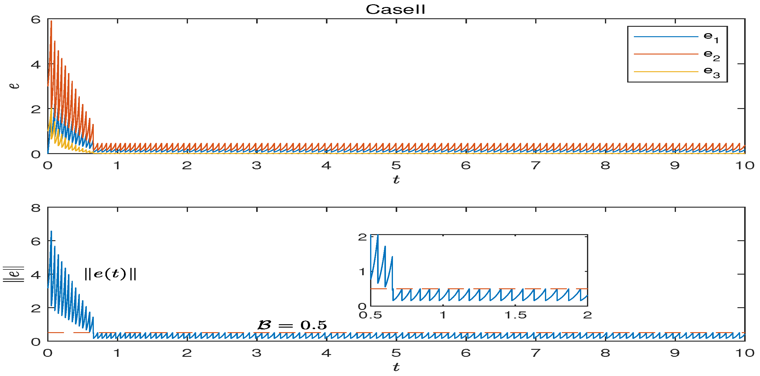
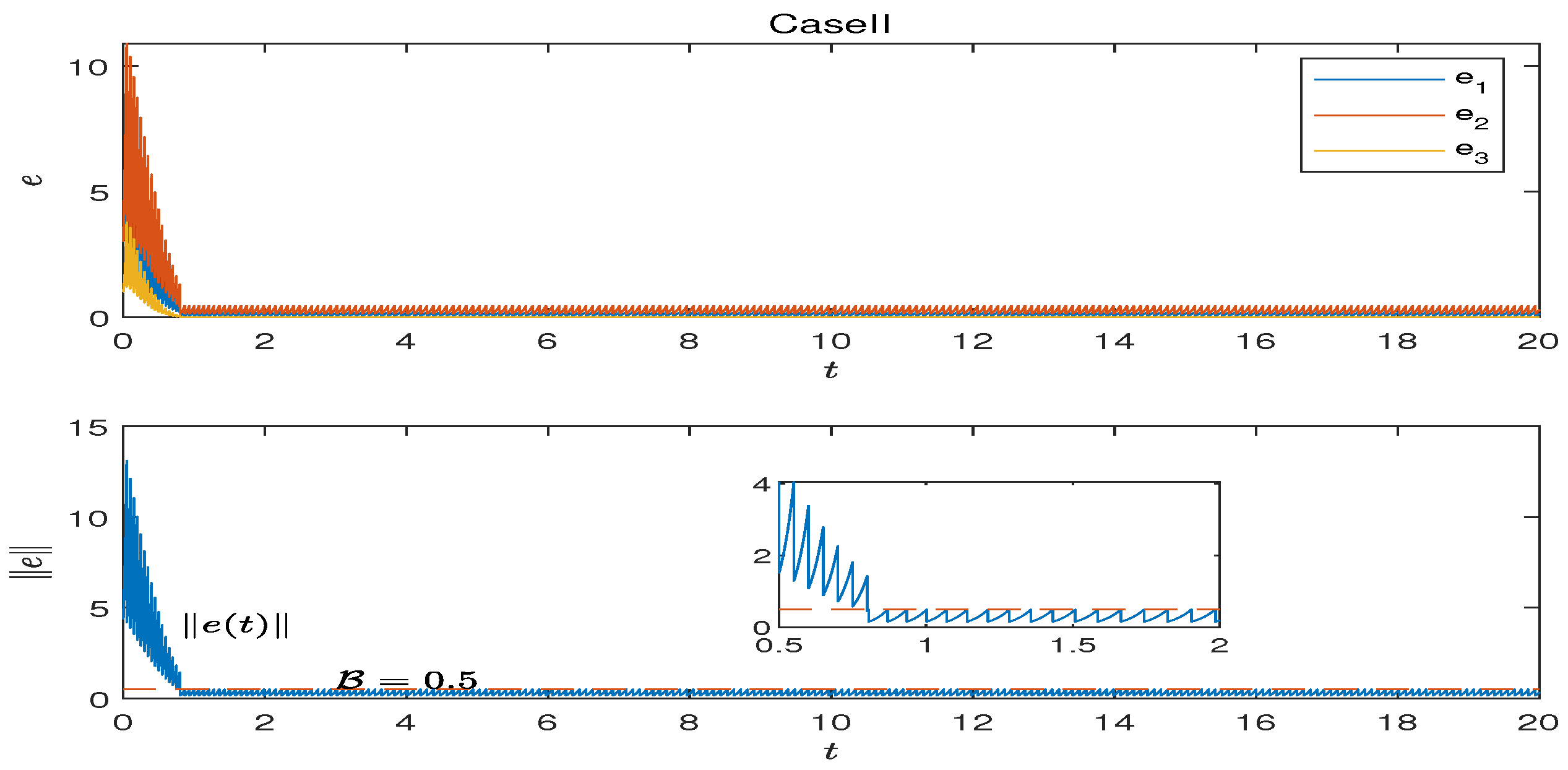
Case-I. FTPIS w.r.t. $\mathcal{B}$ via T-IC: For a bound $\mathcal{B}=0.5$ and the system (73) with $\varphi \left(t\right)={\displaystyle \frac{10}{1+t^2}}$ and $\xi ={(1,0,1.5)}^T$ and $\eta ={(1,3,2.5)}^T$ as the initial states, T-IC $u={\sum }_{k=1}^{\infty }\delta (t-t_k)Kx$ with $t_0=0$ is set to satisfy the algorithm:

$$\begin{array}{c}\hfill \left\{\begin{array}{c}K=-0.68I;\hfill \\ t_k=t_{k-1}+{\displaystyle \frac{-\gamma -d}{\alpha }}=t_{k-1}+0.0500,1\le k\le {\tilde{k}}_{min}^{\left(1\right)},{\tilde{k}}_{min}^{\left(1\right)}=\left[{\displaystyle \frac{1}{-\gamma }}ln{\displaystyle \frac{{\lambda }_{min}\left(P\right){\parallel \mathcal{B}\parallel }^2}{U(\xi ,\eta )e^{-d}}}\right]=94;\hfill \\ t_k=t_{k-1}+0.0505,k>{\tilde{k}}_{min}^{\left(1\right)}=94,\hfill \end{array}\right.\end{array}$$

(75)

where ${\tilde{k}}_{min}^{\left(1\right)}=94$ with $d=2ln0.32=-2.2789$, $\gamma =0.015>0$.

By Theorem 3, then, Lorenz system (73) is FTPIS w.r.t. $\mathcal{B}$ by T-IC satisfying (75) with the settling time ${\mathcal{S}}^{\left(1\right)}(\xi -\eta ,\mathcal{B},T)\le t_{{\tilde{k}}_{min}^{\left(1\right)}}=4.7$. The simulation is given in Figure 1.

Note: Due to the conservativeness of T-IC algorithm (75) (see Remark 5 (iii)), the real settling time of T-IC in the simulation is ${\mathcal{S}}^{\left(1\right)}(\xi -\eta ,\mathcal{B},T)=t_{k_{min}^{\left(1\right)}}=0.85$ with $k_{min}^{\left(1\right)}=17$.

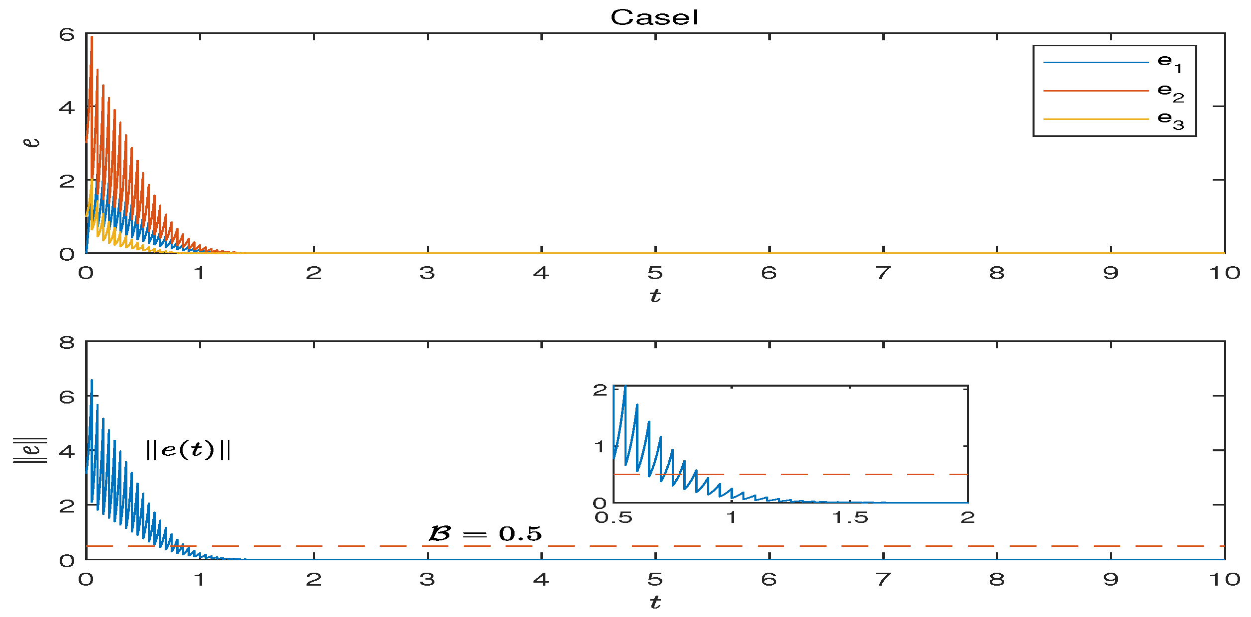
Case-II. FTPIS w.r.t. $\mathcal{B}$ via TS-IC: For the bound $\mathcal{B}=0.5$ and (73) with same $\varphi \left(t\right)$ and the initial states as in Case-I, i.e., $\varphi \left(t\right)={\displaystyle \frac{10}{1+t^2}}$, $\xi ={(1,0,1.5)}^T$, and $\eta ={(1,3,2.5)}^T$, TS-IC $u={\sum }_{k=1}^{\infty }\delta (t-t_k)Kx$ with $t_0=0$ is set to satisfy the algorithm:

$$\begin{array}{c}\hfill \left\{\begin{array}{c}K=-0.68I;\hfill \\ t_k=t_{k-1}+{\displaystyle \frac{-\gamma -d}{\alpha }}=t_{k-1}+0.0500,1\le k\le k_{min}^{\left(2\right)},k_{min}^{\left(2\right)}\triangleq min\{k:\parallel e\left(t_k\right)\parallel \le \mathcal{B}\},\hfill \\ t_k=min\{s:s>t_{k-1},\parallel e\left(s\right)\parallel \ge \mathcal{B}\},k>k_{min}^{\left(2\right)},\hfill \end{array}\right.\end{array}$$

(76)

where $d=2ln0.32=-2.2789$ and $\gamma =0.015>0$.

By Theorem 4, the system (73) is FTPIS w.r.t. $\mathcal{B}$ by TS-IC satisfying (76) with the settling time ${\mathcal{S}}^{\left(2\right)}(\xi -\eta ,\mathcal{B},T)=t_{k_{min}^{\left(2\right)}}=0.65$ with $k_{min}^{\left(2\right)}=13$. The simulation is given in Figure 2.

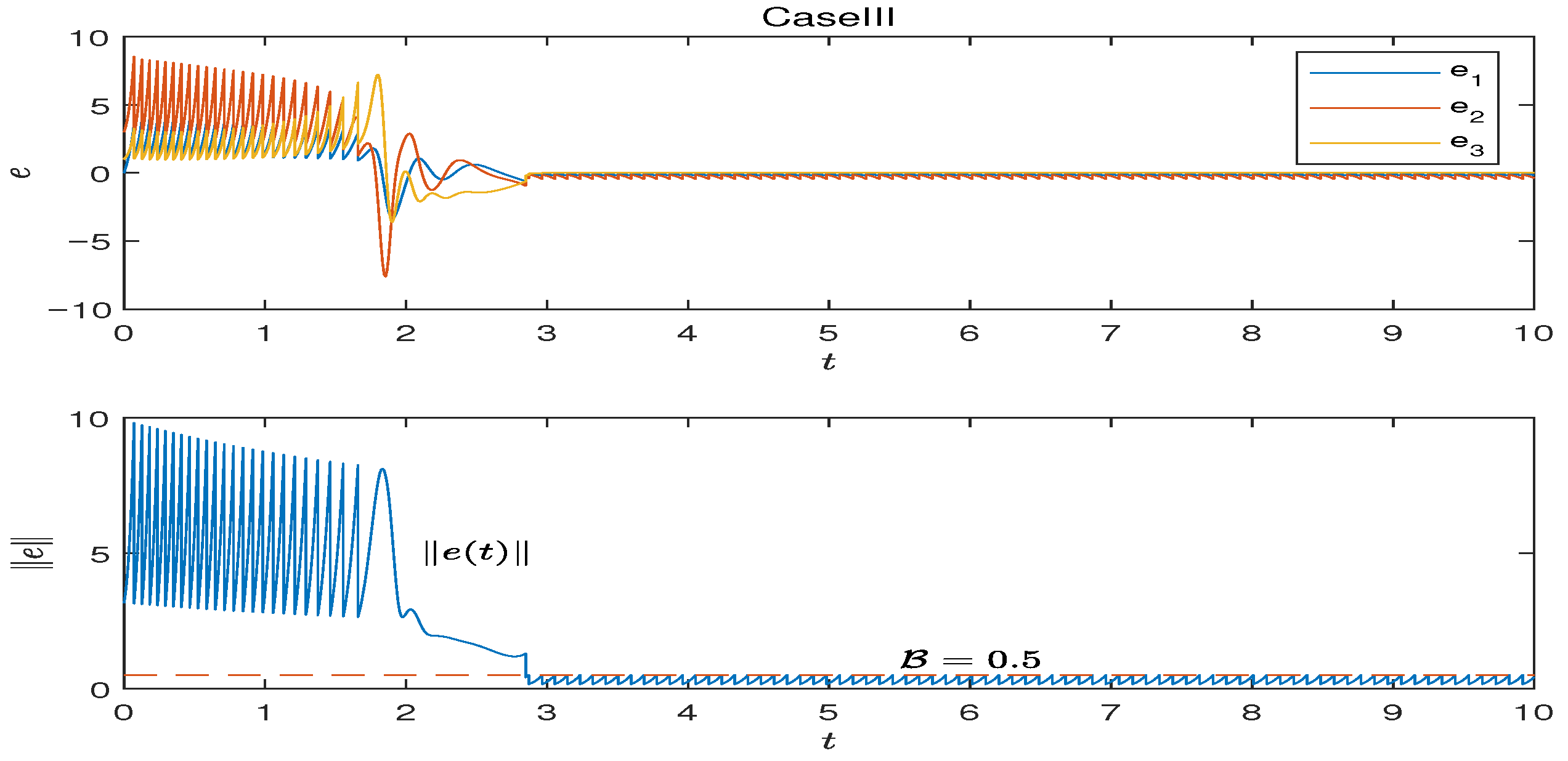
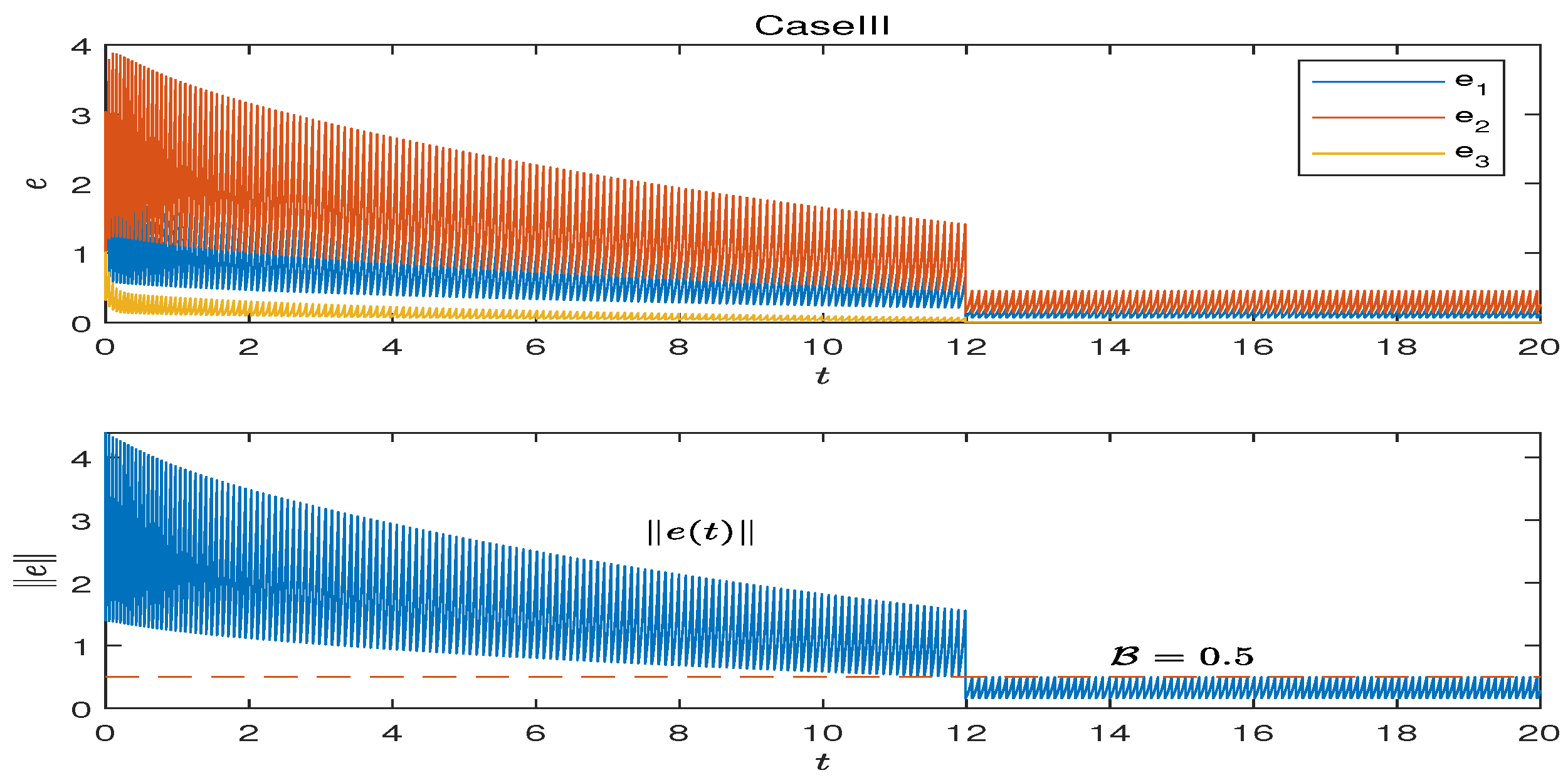
Case-III. FTPIS w.r.t. $\mathcal{B}$ via S-IC: For the bound $\mathcal{B}=0.5$ and (73) with with same $\varphi \left(t\right)$ and the initial states as in Case-I and Case-II, i.e., $\varphi \left(t\right)={\displaystyle \frac{10}{1+t^2}}$, $\xi ={(1,0,1.5)}^T$, and $\eta ={(1,3,2.5)}^T$, S-IC $u={\sum }_{k=1}^{\infty }\delta (t-t_k)Kx$ with $t_0=0$ is set to satisfy the S-IC algorithm:

$$\begin{array}{c}\hfill \left\{\begin{array}{c}K=-0.68I;\hfill \\ t_k=min\{t:t\in {\mathrm{\Psi }}_{k-1}\},if{\mathrm{\Psi }}_{k-1}\ne Ø,\mathrm{otherwise}{t}_k=t_{k-1}+\mathrm{\Delta },\hfill \\ 1\le k\le k_{min}^{\left(3\right)},k_{min}^{\left(3\right)}\triangleq min\{k:\parallel e\left(t_k\right)\parallel \le \mathcal{B}\};\hfill \\ t_k=min\{s:s>t_{k-1},\parallel e\left(s\right)\parallel \ge \mathcal{B}\},k>k_{min}^{\left(3\right)},\hfill \end{array}\right.\end{array}$$

(77)

where ${\mathrm{\Psi }}_0=\{t:t\in (t_0,t_0+\mathrm{\Delta }],\parallel e\left(t\right)\parallel \ge e^{{\displaystyle \frac{-\gamma -d}{2}}}\parallel e\left(t_0\right)\parallel \}$, ${\mathrm{\Psi }}_{k-1}=\{t:t\in (t_{k-1},t_{k-1}+\mathrm{\Delta }],\parallel e\left(t\right)\parallel \ge e^{{\displaystyle \frac{-\gamma }{2}}}\parallel e\left(t_{k-1}\right)\parallel \}$ for $k\ge 2$, $d=2ln0.32=-2.2789$, $\gamma =0.015>0$, and the check-period $\mathrm{\Delta }=1>{\displaystyle \frac{-d}{\alpha }}=0.0505$. By Theorem 5, the system (73) is FTPIS w.r.t. $\mathcal{B}$ by S-IC satisfying (77) with the settling time ${\mathcal{S}}^{\left(3\right)}(\xi -\eta ,\mathcal{B},T)=t_{k_{min}^{\left(3\right)}}=2.8491$ with $k_{min}^{\left(3\right)}=26$. The simulation is given in Figure 3.

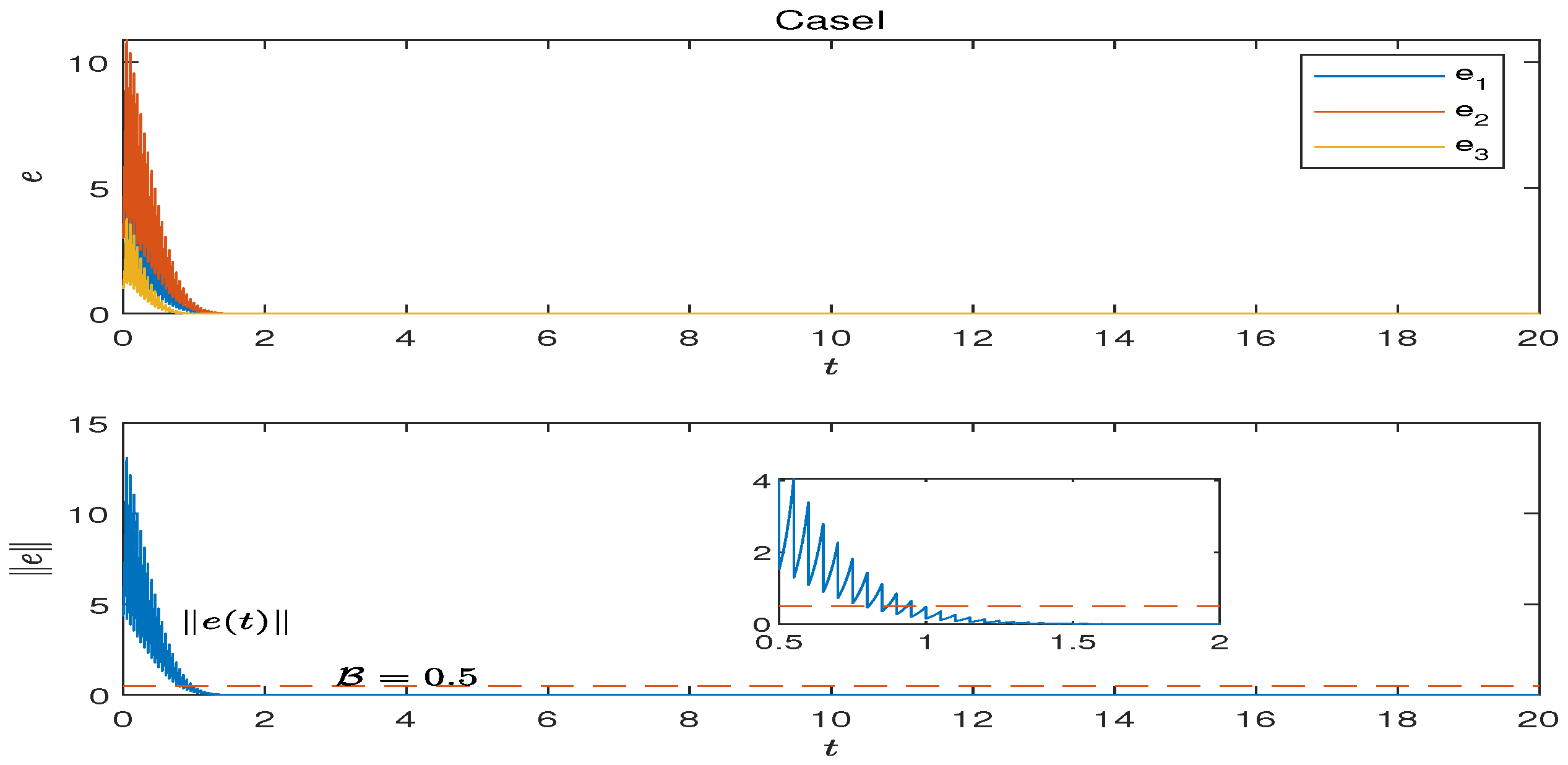
Comparison among T-IC, S-IC, and TS-IC: From Figure 1, Figure 2 and Figure 3. In the simulations, the FTPIS of Lorenz system (73) can be achieved by T-IC, TS-IC, and S-IC, respectively. For more comparison, we give the simulations under different initial conditions. Figure 4, Figure 5 and Figure 6 are the simulations of Case-I and Case-III under different initial conditions. Here, in Figure 4, Figure 5 and Figure 6, $\xi ={(1,0,1.5)}^T$ and $\eta ={(4,3,2.5)}^T$.

Here, the performances including the settling time $S(\xi -\eta ,\mathcal{B},T)$ (here, $\mathcal{S}(\xi -\eta ,\mathcal{B},T)=t_{k_{min}}$), the minimum number $k_{min}$ of impulses required for achieving settling time, and the total number of impulses $N(0,t]$ during $(0,t]$, and the impulse frequency (I.F.) ${\mathcal{F}}_I(0,t]$ during $(0,t]$, are used to give the comparison.

Table 1. Data for T-IC satisfying (75), TS-IC satisfying (76), and S-IC satisfying (77), where $\xi ={(1,0,1.5)}^T$, $\eta ={(1,3,2.5)}^T$, $\mathcal{B}=0.5$, and the simulations refer to Figure 1, Figure 2 and Figure 3.

Impulsive Control	T-IC	TS-IC	S-IC
$S(\xi -\eta ,\mathcal{B},T)=t_{k_{min}}$	0.85	0.65	2.8491
$k_{min}$	17	13	26
$N(0,10]$	199	119	103
${\mathcal{F}}_I(0,10]$	199/10	119/10	103/10

is the data collected from the simulations of Figure 1, Figure 2 and Figure 3. Additionally,

Table 2. Data for T-IC satisfying (75), TS-IC satisfying (76), and S-IC satisfying (77), where $\xi ={(1,0,1.5)}^T$, $\eta ={(4,3,2.5)}^T$, $\mathcal{B}=0.5$, and the simulations refer to Figure 4, Figure 5 and Figure 6.

Impulsive Control	T-IC	TS-IC	S-IC
$S(\xi -\eta ,\mathcal{B},T)=t_{k_{min}}$	1.0	0.8	11.9835
$k_{min}$	20	16	139
$N(0,10]$	397	224	224
${\mathcal{F}}_I(0,10]$	397/20	224/20	224/2

is from the simulations of Figure 4, Figure 5 and Figure 6. From Table 1 and Table 2, one can see that TS-IC performs best in terms of the shortest settling time and the least number of impulses required to reach the settling time. Additionally, the impulse frequency of TS-IC is close to that of S-IC, but the latter has the longest settling time. Therefore, the result of Theorem 6 is verified.

Remark 9.

From Example 1, among T-IC, TS-IC, and S-IC, the TS-IC has advantages to achieve FTPIS, including the shortest settling time, the least number of impulses required for achieving the settling time, and almost the lowest I.F. It is also noted that T-IC is the strongest impulsive control with maximum total number of impulses, highest I.F., and the minimum error when entering into the target region $\parallel e\left(t\right)\parallel \le \mathcal{B}$, than S-IC and TS-IC. S-IC has the lowest I.F., but S-IC has the longest settling time.

6. Conclusions

In this paper, the finite-time practical incremental stability (FTPIS) for impulsive systems and the FTPIS-based impulsive control design have been studied. The notions of FTPIS and finite-time practical stability (FTPS) were proposed. By using the Lyapunov-like function method, criteria of FTPIS and FTPIS settling time estimates were derived. The results were used to design FTPIS-based impulsive control. Three types of impulsive control, including time-triggered impulsive control (T-IC), time-state-triggered impulsive control (TS-IC), and state-triggered impulsive control (S-IC), have been designed respectively for FTPIS. One example on the practical finite-time tracking was presented for the effectiveness of theoretical results. Both theoretical results and numerical simulations have shown that TS-IC can achieve the best performance than T-IC and S-IC with the shortest settling time, the least number of impulsive control required to reach the settling time, and almost the lowest impulse frequency. Moreover, the designed TS-IC improves the mechanism of impulsive control in the literature, which is either time-triggered or state-triggered. The proposed FTPIS-based impulsive control including TS-IC and S-IC may be a control tool for FTS of practical systems with uncertainties and disturbances. For the future work, the FTPIS-based impulsive control for finite-time load frequency control of microgrids and the precision control of missile dynamics will be possible application areas.

References

1. Fromion, V.; Monaco, S.; Normand-Cyrot, D. Asymptotic properties of incrementally stable systems. IEEE Trans. Autom. Control 1996, 41, 721–723. [Google Scholar] [CrossRef] [Scilit]
2. Fromion, V.; Scorletti, G.; Ferreres, G. Nonlinear performance of a PI controlled missile: An explanation. Int. J. Robust Nonlinear Control 1999, 9, 485–518. [Google Scholar] [CrossRef]
3. Angeli, D. A Lyapunov approach to incremental stability properties. IEEE Trans. Autom. Control 2002, 47, 410–421. [Google Scholar] [CrossRef] [Scilit]
4. Franci, A.; Chaillet, A.; Pasillas-Lepine, W. Phase-locking between Kuramoto oscillators: Robustness to time-varying natural frequencies. In Proceedings of the IEEE Conference on Decision and Control, Atlanta, GA, USA, 15–17 December 2010; IEEE: New York, NY, USA, 2010; pp. 1587–1592. [Google Scholar]
5. Girard, A.; Pola, G.; Tabuada, P. Approximately bisimilar symbolic models for incrementally stable switched systems. IEEE Trans. Autom. Control 2009, 55, 116–126. [Google Scholar] [CrossRef] [Scilit]
6. Zamani, M.; van de Wouw, N. Controller synthesis for incremental stability: Application to symbolic controller synthesis. In Proceedings of the European Control Conference, Zurich, Switzerland, 17–19 July 2013; IEEE: New York, NY, USA, 2013; pp. 2198–2203. [Google Scholar]
7. Richter, J.H.; Heemels, W.P.M.H.; van de Wouw, N.; Lunze, J. Reconfigurable control of piecewise affine systems with actuator and sensor faults: Stability and tracking. Automatica 2011, 47, 678–691. [Google Scholar] [CrossRef] [Scilit]
8. Hamadeh, A.; Stan, G.-B.; Sepulchre, R.; Goncalves, J. Global state synchronization in networks of cyclic feedback systems. IEEE Trans. Autom. Control 2012, 57, 478–483. [Google Scholar] [CrossRef] [Scilit]
9. Russo, G.; di Bernardo, M. Contraction theory and master stability function: Linking two approaches to study synchronization of complex networks. IEEE Trans. Circuits Syst. II 2009, 56, 177–181. [Google Scholar] [CrossRef] [Scilit]
10. Liu, T.; Hill, D.J.; Zhao, J. Output synchronization of dynamical networks with incrementally dissipative nodes and switching topology. IEEE Trans. Circuits Syst. I Regul. Pap. 2015, 62, 2312–2323. [Google Scholar] [CrossRef] [Scilit]
11. Rantzer, A. A performance criterion for antiwindup compensators. Eur. J. Control 2000, 6, 449–452. [Google Scholar] [CrossRef] [Scilit]
12. Giaccagli, M.; Astolfi, D.; Andrieu, V.; Marconi, L. Incremental stabilization of cascade nonlinear systems and harmonic regulation: A forwarding-based design. IEEE Trans. Autom. Control 2024, 69, 4828–4835. [Google Scholar] [CrossRef] [Scilit]
13. Ruffer, B.S.; van de Wouw, N.; Mueller, M. Convergent systems vs. incremental stability. Syst. Control Lett. 2013, 62, 277–285. [Google Scholar] [CrossRef] [Scilit]
14. Waitman, S.; Bako, L.; Massioni, P.; Scorletti, G.; Fromion, V. Incremental stability of Lur’e systems through piecewise-affine approximations. IFAC-PapersOnLine 2017, 50, 1673–1679. [Google Scholar] [CrossRef] [Scilit]
15. Lohmiller, W.; Slotine, J.-J.E. On contraction analysis for nonlinear systems. Automatica 1998, 34, 683–696. [Google Scholar] [CrossRef] [Scilit]
16. Lohmiller, W.; Slotine, J.-J.E. Control system design for mechanical systems using contraction theory. IEEE Trans. Autom. Control 2000, 45, 984–989. [Google Scholar] [CrossRef] [Scilit]
17. Jouroy, J. A simple extension of contraction theory to study incremental stability properties. In Proceedings of the European Control Conference, Cambridge, UK, 1–4 September 2003; IEEE: New York, NY, USA, 2003. [Google Scholar]
18. Jouroy, J.; Fossen, T.I. A tutorial on incremental stability analysis using contraction theory. Model. Identif. Control 2010, 31, 93–106. [Google Scholar]
19. Fiore, D.; Hogan, S.J.; di Bernardo, M. Contraction analysis of switched systems via regularization. Automatica 2016, 73, 279–288. [Google Scholar] [CrossRef] [Scilit]
20. Rifai, K.E.; Slotine, J.-J.E. Compositional contraction analysis of resetting hybrid systems. IEEE Trans. Autom. Control 2006, 51, 1536–1541. [Google Scholar] [CrossRef] [Scilit]
21. Jiang, H.; Bi, Q. Contraction theory based synchronization analysis of impulsively coupled oscillators. Nonlinear Dyn. 2012, 67, 781–791. [Google Scholar] [CrossRef] [Scilit]
22. Li, X.; Bohner, M.; Wang, C.-K. Impulsive differential equations: Periodic solutions and applications. Automatica 2015, 52, 173–178. [Google Scholar] [CrossRef] [Scilit]
23. Xu, H.; Zhu, Q.; Zheng, W.X. Exponential stability of stochastic nonlinear delay systems subject to multiple periodic impulses. IEEE Trans. Autom. Control 2024, 69, 2621–2628. [Google Scholar] [CrossRef] [Scilit]
24. Liu, B.; Xu, B.; Sun, Z. Incremental stability and contraction via impulsive control for continuous-time dynamical systems. Nonlinear Anal. Hybrid Syst. 2021, 39, 100981. [Google Scholar] [CrossRef] [Scilit]
25. Kawano, Y.; Cao, M. Contraction analysis of virtually positive systems. Syst. Control Lett. 2022, 168, 105358. [Google Scholar] [CrossRef] [Scilit]
26. Gokul, P.; Soundararajan, G.; Kashkynbayev, A.; Rakkiyappan, R. Finite-time contractive stability for fractional-order nonlinear systems with delayed impulses: Applications to neural networks. Neurocomputing 2024, 610, 128599. [Google Scholar] [CrossRef] [Scilit]
27. Zhang, L.; Guo, W. Finite-time contraction stability and optimal control for mosquito population suppression model. Mathematics 2024, 12, 22. [Google Scholar] [CrossRef] [Scilit]
28. Yang, X.; Li, X. Finite-time stability of nonlinear impulsive systems with applications to neural networks. IEEE Trans. Neural Netw. Learn. Syst. 2023, 34, 243–251. [Google Scholar] [CrossRef] [Scilit] [PubMed]
29. Bhat, S.P.; Bernstein, D.S. Finite-time stability of continuous autonomous systems. SIAM J. Control Optim. 2000, 38, 751–766. [Google Scholar] [CrossRef] [Scilit]
30. Moulay, E.; Perruquetti, W. Finite time stability and stabilization of a class of continuous systems. J. Math. Anal. Appl. 2006, 323, 1430–1443. [Google Scholar] [CrossRef] [Scilit]
31. Hong, Y.; Jiang, Z.-P.; Feng, G. Finite-time input-to-state stability and applications to finite-time control design. SIAM J. Control Optim. 2010, 48, 4395–4418. [Google Scholar] [CrossRef] [Scilit]
32. He, X.; Li, X.; Nieto, J.J. Finite-time stability and stabilization for time-varying systems. Chaos Solit. Fractals 2021, 148, 111076. [Google Scholar] [CrossRef] [Scilit]
33. Yu, X.; Yin, J.; Khoo, S. Generalized Lyapunov criteria on finite-time stability of stochastic nonlinear systems. Automatica 2019, 107, 183–189. [Google Scholar] [CrossRef] [Scilit]
34. Yan, Z.; Zhou, X.; Chang, G.; Gao, Z. Finite-time annular domain stability and stabilization of stochastic systems with semi-Markovian switching. IEEE Trans. Autom. Control 2023, 68, 6247–6254. [Google Scholar] [CrossRef] [Scilit]
35. Zhu, Z.; Liao, S.; Jia, F. Nonovershooting prescribed finite-time control for nonlinear pure-feedback systems. Complex Syst. Stab. Control 2025, 1, 4. [Google Scholar]
36. Amato, F.; Ambrosino, R.; Ariola, M.; Cosentino, C. Finite-time stability of linear time-varying systems with jumps. Automatica 2009, 45, 1354–1358. [Google Scholar] [CrossRef] [Scilit]
37. Cheng, M.; Zhao, J.; Xie, X.; Sun, Z.-Y. A novel finite-time stability criteria and controller design for nonlinear impulsive systems. Appl. Math. Comput. 2024, 479, 128876. [Google Scholar] [CrossRef] [Scilit]
38. Liang, Z.; Liu, X. Finite-time hybrid impulsive formation tracking control of multi-agent systems via aperiodic intermittent communication. ISA Trans. 2024, 155, 20–33. [Google Scholar] [CrossRef] [Scilit] [PubMed]
39. Xing, Y.; He, X.; Li, X. Finite-time stabilization of nonlinear time-varying systems involving impulsive action. Commun. Nonlinear Sci. Numer. Simul. 2024, 131, 107818. [Google Scholar] [CrossRef] [Scilit]
40. Jiang, M.-H.; Liu, B.; Mo, S.-H.; Liu, D.-H. Finite-time practical stability of impulsive systems with application to design of impulsive control. Asian J. Control 2025. [Google Scholar] [CrossRef] [Scilit]
41. Zhang, T.; Cao, J.; Li, X. Lyapunov conditions for finite-time input-to-state stability of impulsive switched systems. IEEE/CAA J. Autom. Sin. 2024, 11, 1057–1059. [Google Scholar] [CrossRef] [Scilit]
42. Fu, L.; Peng, S.; Wang, J. Semiglobal finite-time stability of impulsive systems. IEEE Trans. Circuits Syst. I Regul. Pap. 2025, 72, 932–940. [Google Scholar] [CrossRef] [Scilit]
43. Li, X.; Ho, D.W.C.; Cao, J. Finite-time stability and settling-time estimation of nonlinear impulsive systems. Automatica 2019, 99, 361–368. [Google Scholar] [CrossRef] [Scilit]
44. Ai, Z.; Zong, G. Finite-time stochastic input-to-state stability of impulsive switched stochastic nonlinear systems. Appl. Math. Comput. 2014, 245, 462–473. [Google Scholar]
45. Hu, H.; Gao, B.; Xu, L. Finite-time and fixed-time attractiveness for nonlinear impulsive systems. IEEE Trans. Autom. Control 2022, 67, 5586–5593. [Google Scholar] [CrossRef] [Scilit]
46. Liu, Y.; Liu, B.; Fu, Z.; Yang, X. Exponential input-to-state stability of load frequency control system of island microgrid with time-delay under aperiodic intermittent control. Asian J. Control 2025, 27, 2940–2949. [Google Scholar] [CrossRef] [Scilit]
47. Dashkovskiy, S.; Feketa, P. Input-to-state stability of impulsive systems and their networks. Nonlinear Anal. Hybrid Syst. 2017, 26, 190–200. [Google Scholar] [CrossRef] [Scilit]
48. Mancilla-Aguilar, J.L.; Haimovich, H.; Feketa, P. Uniform stability of nonlinear time-varying impulsive systems with eventually uniformly bounded impulse frequency. Nonlinear Anal. Hybrid Syst. 2020, 38, 100933. [Google Scholar] [CrossRef] [Scilit]
49. Li, P.; Liu, B.; Jiang, M.-H.; Cheng, J.; Wang, X. Input-delayed time/event-triggered intermittent control for incremental stability. ISA Trans. 2026. [Google Scholar] [CrossRef] [Scilit] [PubMed]
50. Yang, T. Impulsive Control Theory; Springer: Berlin, Germany, 2001. [Google Scholar]
51. Haddad, W.M.; Chellaboina, V.-S.; Nersesov, S.G. Impulsive and Hybrid Dynamical Systems; Princeton University Press: Princeton, NJ, USA, 2006. [Google Scholar]
52. Ai, Z.; Peng, L.; Zong, G.; Shi, K. Impulsive control for nonlinear systems under DoS attacks: A dynamic event-triggered method. IEEE Trans. Circuits Syst. II Express Briefs 2022, 69, 3839–3843. [Google Scholar] [CrossRef] [Scilit]
53. Chen, W.-H.; Xu, W.; Zheng, W.X. Sliding-mode-based impulsive control for a class of time-delay systems with input disturbance. Automatica 2024, 164, 111633. [Google Scholar] [CrossRef] [Scilit]
54. Liu, B.; Sun, Z.; Li, M.; Liu, D.-N. Stabilization via event-triggered impulsive control with constraints for switched stochastic systems. IEEE Trans. Cybern. 2022, 52, 11834–11846. [Google Scholar] [CrossRef] [Scilit] [PubMed]
55. Lakshmikantham, V.; Bainov, D.D.; Simeonov, P.S. Theory of Impulsive Differential Equations; World Scientific: Singapore, 1989. [Google Scholar]
Figure 1. (Top) The error state e ( t ) = x ( t , ξ ) y ( t , η ) under T-IC satisfying (75) for Lorenz system (73), where x ( t , ξ ) and y ( t , η ) are the solutions of the system (74) with initial states ξ and η , respectively. (Bottom) FTPIS of Lorenz system (73) via T-IC satisfying (75).
Mathematics 14 01657 g001
Figure 2. (Top) The error state e ( t ) = x ( t , ξ ) y ( t , η ) under TS-IC satisfying (76) for Lorenz system (73), where x ( t , ξ ) and y ( t , η ) are the solutions of the system (68) with initial states ξ and η , respectively. (Bottom) FTPIS of Lorenz system (73) via TS-IC satisfying (76).
Mathematics 14 01657 g002
Figure 3. (Top) The error state e ( t ) = x ( t , ξ ) y ( t , η ) under S-IC satisfying (77) for Lorenz system (73), where x ( t , ξ ) and y ( t , η ) are the solutions of (74) with initial states ξ and η , respectively. (Bottom) FTPIS of Lorenz system (73) via S-IC satisfying (77).
Mathematics 14 01657 g003
Figure 4. (Top) The error state e ( t ) = x ( t , ξ ) y ( t , η ) under T-IC satisfying (75) for Lorenz system (73), where x ( t , ξ ) and y ( t , η ) are the solutions of the system (74) with ξ = ( 1 , 0 , 1.5 ) T , η = ( 4 , 3 , 2.5 ) T , respectively. (Bottom) FTPIS of Lorenz system (73) via T-IC satisfying (75).
Mathematics 14 01657 g004
Figure 5. (Top) The error state e ( t ) = x ( t , ξ ) y ( t , η ) under TS-IC satisfying (76) for Lorenz system (73), where x ( t , ξ ) and y ( t , η ) are the solutions of the system (68) with ξ = ( 1 , 0 , 1.5 ) T , η = ( 4 , 3 , 2.5 ) T , respectively. (Bottom) FTPIS of Lorenz system (73) via TS-IC satisfying (76).
Mathematics 14 01657 g005
Figure 6. (Top) The error state e ( t ) = x ( t , ξ ) y ( t , η ) under S-IC satisfying (77) for Lorenz system (73), where x ( t , ξ ) and y ( t , η ) are the solutions of (74) with ξ = ( 1 , 0 , 1.5 ) T , η = ( 4 , 3 , 2.5 ) T , respectively. (Bottom) FTPIS of Lorenz system (73) via S-IC satisfying (77).
Mathematics 14 01657 g006