Dual-Channel Financing with Bank Credit and 3PL Direct Financing: Operational and Financing Decisions in a Capital-Constrained Supply Chain

Abstract

This study examines how bank financing and direct financing provided by a third-party logistics (3PL) firm affect the operational and financing decisions of a capital-constrained retailer. It focuses on a dual-channel financing setting in which both funding sources are available and investigates whether the retailer uses them simultaneously, how creditor priority affects equilibrium outcomes, and how procurement cost and logistics pricing shape financing choices. A Stackelberg game model is developed for a supply chain comprising a retailer, a 3PL firm, and a bank. Two benchmark settings, namely bank financing only and direct 3PL financing only, are first analyzed. The study then examines the dual-channel financing equilibrium when the 3PL firm acts as the senior creditor and further extends the model to consider bank seniority and endogenous logistics pricing. When the 3PL firm is the senior creditor, the retailer does not use both funding sources simultaneously in equilibrium; instead, it chooses either bank financing only or direct 3PL financing only. The 3PL firm prefers bank financing when logistics pricing is low and procurement cost is high, whereas it prefers direct financing when logistics pricing is high or when both logistics pricing and procurement cost are low. When logistics pricing is endogenous, the optimal lending rate set by the 3PL firm is zero. This study extends the literature on 3PL financing by explicitly incorporating a dual-channel financing structure that includes both bank credit and direct 3PL lending. It highlights the strategic role of creditor priority and shows how procurement cost and logistics pricing jointly shape the financing equilibrium, thereby providing managerial insights into financing design and operational decision-making in capital-constrained supply chains.

1. Introduction

Small and medium-sized enterprises (SMEs) are cornerstones of economic development. They play an essential role in driving economic growth, fostering innovation, generating employment, and enhancing social welfare. In China, SMEs contribute more than 50% of tax revenue, more than 60% of GDP, more than 70% of technological innovation, more than 80% of urban employment, and account for more than 90% of all firms. Despite their economic importance, SMEs often face severe financing constraints. According to a report released by the Guanghua School of Management, Peking University, 34% of Chinese small and micro firms identify cash-flow shortages as a major operational challenge (https://www.gsm.pku.edu.cn/info/1740/24093.htm (accessed on 8 May 2026)). More broadly, capital shortages remain a widespread challenge worldwide, especially for supply chain firms that must make procurement and production decisions under working-capital constraints [1,2]. According to the World Bank Enterprise Surveys, which covered more than 195,000 firms in 155 economies in 2023, 15.3% of firms regard access to finance as a major constraint; this proportion is substantially higher in some developing economies (https://www.enterprisesurveys.org/en/data/exploretopics/finance (accessed on 8 May 2026)). Traditionally, bank loans have served as the primary external funding source for capital-constrained firms and therefore play an important role in supply chain financing [3,4]. However, stringent credit screening and high collateral requirements substantially limit SMEs’ access to bank credit. According to the same World Bank survey, approximately 74.7% of loans require collateral, and the collateral value is, on average, 1.93 times the loan amount (https://www.enterprisesurveys.org/en/data/exploretopics/finance (accessed on 8 May 2026)). As a result, SMEs increasingly seek alternative financing channels to alleviate financial pressure.

Against this background, logistics finance has developed rapidly alongside the expansion of global trade. By integrating logistics and finance, logistics finance provides funding, settlement, and risk-management services while reducing transaction costs and improving financing efficiency (https://www.chinairn.com/news/20230919/144556389.shtml (accessed on 8 May 2026)). Recent market reports suggest that China’s logistics finance market continues to expand rapidly and may reach tens of trillions of RMB (https://www.chinairn.com/scfx/20241024/151547750.shtml (accessed on 8 May 2026)). In this process, third-party logistics (3PL) firms have gradually moved beyond their traditional role as logistics service providers and have become active participants in supply chain finance. This evolution is economically intuitive. On the one hand, 3PL firms possess detailed knowledge of cargo flows and operational processes, which may reduce financing risk and improve capital allocation efficiency (https://www.mckinsey.com.cn/ (accessed on 8 May 2026)). On the other hand, as the physical controllers of pledged goods, 3PL firms may have inherent advantages in risk control and asset management. Moreover, by providing financing services, 3PL firms can deepen customer relationships, expand their value-added services, and strengthen their competitive position in the supply chain (https://cj.sina.com.cn/articles/view/3958636400/ebf3ff7001900ho1h (accessed on 8 May 2026)).

These developments are also evident in practice. Many large logistics providers, including UPS, FedEx, and DHL, have incorporated financing services into their business models. For example, UPS Capital announced in 2018 that it would expand its cargo finance services for U.S. importers by increasing advance rates, extending repayment terms, and offering unsecured credit lines (https://ajot.com/news/ups-capital-announces-ups-capital-cargo-finance-service-enhancements (accessed on 8 May 2026)). In China, major logistics firms, including Eternal Asia, Sinotrans, and SF Express, have also introduced various supply chain finance products. SF Express, for instance, offers warehouse financing, order financing, micro-loans, and factoring services to capital-constrained firms and has further developed order-based financing solutions for customers engaged in deeper supply chain cooperation (https://maimai.cn/article/detail?fid=1421375850&efid=I4yjsV-YDB3H1-5hLJBC0Q (accessed on 8 May 2026)). These practices suggest that direct financing provided by 3PL firms has become an increasingly important short-term financing arrangement for SMEs.

The growing role of 3PL firms in supply chain finance has attracted increasing academic attention [5,6]. Existing studies have shown that 3PL financing can improve operational efficiency, facilitate risk sharing, and enhance supply chain performance. Nevertheless, several important questions remain unresolved. First, most existing studies assume that a capital-constrained firm chooses either bank financing or direct 3PL financing, whereas relatively little attention has been paid to settings in which both financing channels are simultaneously available. Although some studies allow a retailer to borrow from both a bank and a supplier [7,8], relatively little is known about dual-channel financing in which a capital-constrained retailer can access both bank financing and direct 3PL financing. Second, the effect of creditor priority on equilibrium financing outcomes remains underexplored. In particular, when the 3PL firm acts as a senior creditor, its lending strategy and the retailer’s financing choice may differ fundamentally from those in conventional bank-financing settings. Third, because 3PL firms often possess pricing power in logistics services, the interaction between logistics pricing and financing terms deserves further investigation.

Against this background, the present study addresses the following related questions: When both bank financing and direct 3PL financing are available, does a capital-constrained retailer use the two funding sources simultaneously or rely on only one of them? How does creditor priority affect the retailer’s financing choice and the 3PL firm’s lending strategy? Under what conditions does the 3PL firm prefer to offer direct financing rather than allow the retailer to rely on bank credit? Moreover, how do procurement cost and logistics pricing jointly influence the equilibrium financing arrangement and the retailer’s ordering decision?

Motivated by these gaps, this study investigates the operational and financing strategies of a capital-constrained retailer in a supply chain comprising a retailer, a 3PL firm, and a bank. The retailer sells products to consumers but lacks sufficient initial capital to finance procurement. The 3PL firm provides logistics services and, when the retailer seeks financing, may also provide direct lending. To better understand the dual-channel financing problem, we first analyze two benchmark cases: bank financing only and direct 3PL financing only. We then examine a dual-channel financing setting in which both financing channels are available. In the main model, the 3PL firm is assumed to be the senior creditor; thus, the retailer repays the 3PL loan before repaying the bank once sales revenue is realized. The retailer decides whether to accept the financing terms offered by the 3PL firm and accordingly chooses its order quantity and borrowing amounts. We further analyze the financing preferences of both parties, the equilibrium financing contract, and the effects of procurement cost and logistics pricing on the financing equilibrium.

Our analysis yields several key insights. We show that, under the benchmark settings, bank financing and direct 3PL financing generate distinct equilibrium implications for ordering and financing decisions. More importantly, in the dual-channel setting with the 3PL firm as the senior creditor, the retailer does not use both financing sources simultaneously in equilibrium; instead, it selects either bank financing only or direct 3PL financing only. The 3PL firm’s financing incentive depends critically on the joint effect of procurement cost and logistics pricing: bank financing is preferred when logistics pricing is relatively low and procurement cost is relatively high, whereas direct 3PL financing becomes more attractive when logistics pricing is high or when both logistics pricing and procurement cost are low. In addition, the extensions reveal that changing creditor priority or endogenizing logistics pricing can substantially alter the equilibrium financing outcome, thereby highlighting the strategic roles of repayment hierarchy and logistics pricing power in supply chain finance.

This study makes three main contributions. First, it extends the literature on 3PL financing by explicitly examining a dual-channel financing setting in which a capital-constrained retailer can access both bank financing and direct 3PL financing. This setting captures an important but underexplored financing arrangement in supply chain practice. Second, it characterizes the financing preferences of the retailer and the 3PL firm and identifies the conditions under which a financing contract can be formed in equilibrium. In particular, the analysis clarifies whether the retailer combines the two funding sources or chooses only one of them when the 3PL firm strategically sets lending terms. Third, the study shows how creditor priority, procurement cost, and logistics pricing jointly shape the financing equilibrium, thereby enriching the literature on the determinants of financing strategies in capital-constrained supply chains. These findings also provide managerial insights for retailers and 3PL firms in designing financing arrangements and operational policies.

From a methodological perspective, the novelty of this paper lies in a stochastic Stackelberg formulation and an equilibrium characterization of dual-channel inventory financing with creditor-priority-dependent repayment rules. Unlike standard single-creditor newsvendor financing models, our formulation explicitly allows the retailer to allocate borrowing between a competitive bank and a 3PL lender while incorporating repayment hierarchy into the payoff functions. This structure generates several analytical results that do not arise in single-channel financing settings. First, under the IFR demand condition, we characterize the retailer’s optimal order quantity and the induced financing threshold under direct 3PL financing. Second, we derive the feasible lending region of the junior creditor and show how creditor priority changes the boundary structure of the retailer’s financing choice. Third, under a uniform demand distribution, we obtain closed-form threshold conditions that separate the bank-financing, direct-3PL-financing, and dual-channel-financing regions. Therefore, the contribution is not a numerical algorithm but rather an analytical equilibrium characterization of a stochastic financing game with a creditor-priority-dependent repayment structure.

The remainder of this paper is organized as follows. Section 1 outlines the research background and presents the main research questions. Section 2 reviews the related literature. Section 3 develops the model, examines the two benchmark cases of bank financing only and direct 3PL financing only, and characterizes the equilibrium under dual-channel financing. Section 4 presents several extensions of the main model. Section 5 concludes the paper and suggests avenues for future research. All proof are attached in the Appendix A.

2. Literature Review

This study is related to four streams of literature: the operations–finance interface in supply chains, trade credit and other non-bank financing mechanisms, 3PL financing in supply chain finance, and supply chain coordination through contracts.

The first stream is the literature on the interface between operations management and finance. Early studies on operational decision-making in supply chains mainly focused on settings with uncertain demand but without financial constraints, examining how firms optimize inventory and related operating decisions under demand uncertainty [9,10,11,12]. Following the seminal insight of Modigliani and Miller [13], operational decisions and financing decisions were long treated as largely independent in a perfect capital market. As market competition intensified and the financing difficulties of small and medium-sized enterprises (SMEs) became increasingly prominent, researchers gradually recognized that operational decisions and financing decisions should be jointly analyzed. Buzacott and Zhang [14] was among the first to explicitly study the operational decisions of capital-constrained firms in a bank-financing setting and to highlight the necessity of integrating operations and finance. Subsequent studies further examined this integration from different perspectives, including pre-season production, joint production and financing decisions, hedging, dynamic operational control, and production planning [15,16,17,18,19,20,21,22,23]. In the newsvendor context, Dada and Hu [24] studied the optimal ordering decision of a capital-constrained retailer facing a profit-maximizing bank and proposed a nonlinear loan scheme that partially coordinates the supply chain. Other studies have explored how capital market competition, supply disruption risk, and default risk affect financing and ordering decisions in capital-constrained supply chains [25,26,27]. These studies provide a valuable foundation for understanding operational and financing decisions under bank financing. In our setting, bank financing serves as an important benchmark, while the main focus is on the efficiency of 3PL financing relative to bank financing.

The second stream concerns trade credit and other non-bank financing mechanisms in supply chains. In practice, SMEs often face severe obstacles in obtaining bank loans because they lack sufficient collateral and strong credit histories. As a result, non-bank financing channels such as trade credit have become increasingly important. Empirical evidence shows that trade credit is widely used and economically significant [28,29]. Trade credit refers to a payment arrangement in which the seller allows the buyer to delay payment for purchased products or services [28,30,31]. Starting from the classic EOQ model with delayed payment proposed by Goyal [32], a large body of research has investigated the operational and financial implications of trade credit. Studies have shown that trade credit may mitigate supplier moral hazard, facilitate risk sharing, and improve supply chain efficiency [28,33,34]. Several papers compare trade credit with bank financing and show that trade credit can induce the retailer to purchase more and, under certain conditions, improve supply chain performance [3,4,35,36]. From this perspective, financing provided by a 3PL firm to a downstream capital-constrained retailer can be viewed as a special form of supply chain credit. In addition, with the rapid growth of e-commerce and platform-based supply chains, downstream firms such as large retailers or assemblers have increasingly become financing providers for upstream suppliers or manufacturers. This has motivated studies on buyer financing, purchase-order financing, and related arrangements [25,37,38,39,40]. Unlike these studies, which mainly examine financing provided by downstream firms to upstream firms, our study focuses on financing provided by a 3PL firm to a capital-constrained retailer.

The third stream is the literature on 3PL financing. As 3PL firms have become increasingly involved in financing supply chain participants in practice, 3PL financing has attracted growing attention in the supply chain finance literature. Existing studies suggest that 3PL firms may benefit the supply chain through their relational advantage, disruption-risk management capability, integration of logistics and procurement services, and coordinating role [41,42,43,44]. In particular, Chen and Cai [45] investigated 3PL financing and trade credit for a capital-constrained retailer and showed that, relative to bank financing, 3PL financing can improve the profits of all supply chain members and the entire supply chain. Building on this framework, Hua et al. [46] further incorporated logistics pricing and found that a 3PL firm may offer a lower financing rate to induce a larger order quantity and thereby benefit from higher logistics revenue. Other related studies have examined the operational strategies and coordination conditions in supply chains where a 3PL firm provides financing services [5,47,48]. Zhou et al. [49] compared manufacturer-guaranteed financing and 3PL-guaranteed financing and showed that, when the supply chain is sufficiently cost efficient, all members prefer guaranteed financing to traditional bank financing. They further demonstrated that a longer decision hierarchy can alleviate the free-riding problem among potential guarantors. Although these studies have substantially enriched the literature on 3PL financing, most of them focus on settings in which the capital-constrained firm chooses either bank financing or 3PL financing, but not both. Moreover, relatively limited attention has been paid to the role of the 3PL firm as a guarantor for a retailer’s bank loan, especially when the 3PL firm acts as the channel leader and strategically sets logistics prices or financing terms.

The fourth relevant stream is the literature on supply chain coordination and contracts. Supply chain contracts play a central role in coordinating production, inventory, pricing, and transportation decisions. Common coordinating contracts include wholesale price discount contracts, inventory subsidy agreements, buyback contracts, revenue-sharing contracts, and consignment contracts [50,51,52,53,54,55,56,57,58,59]. Some studies focus on a single contract capable of achieving coordination. For example, Zhang et al. [60] proposed a modified quantity-discount contract based on order quantity and prepayment to coordinate a supply chain with trade credit and a risk-averse manufacturer. Other studies have considered more flexible contracts or compared multiple contract forms [61,62,63,64]. It has also been shown that financing costs, default risk, and bankruptcy propagation may fundamentally affect the effectiveness of coordination contracts [65,66,67]. However, the existing contract literature either does not explicitly consider capital constraints or pays little attention to coordination under 3PL financing. In our setting, direct 3PL financing may coordinate the supply chain under certain conditions because the 3PL firm and the retailer jointly bear part of the demand uncertainty risk.

Overall, the existing literature has made significant progress in understanding the interactions among operational decisions, financing choices, and supply chain coordination. Nevertheless, several important gaps remain. First, although an increasing number of studies have examined financing provided by 3PL firms, most of them focus on settings in which a capital-constrained firm adopts either bank financing or direct 3PL financing, while the possibility of mixed financing has received much less attention. Second, relatively little is known about whether a capital-constrained retailer will simultaneously use bank financing and direct financing from a 3PL firm when both channels are available. Third, the role of creditor seniority in shaping financing equilibrium, operational decisions, and financing preferences under mixed financing remains largely underexplored. To address these gaps, this study investigates the operational and financing decisions of a capital-constrained retailer under bank financing, direct 3PL financing, and mixed financing. It further examines how creditor priority affects equilibrium financing outcomes when the retailer can access both bank credit and direct financing from the 3PL firm. In doing so, this study contributes to the literature on supply chain finance, 3PL financing, and the integration of operations and finance.

3. Model

We consider a supply chain comprising a retailer, a third-party logistics (3PL) firm, and a bank. The capital-constrained retailer relies on the well-capitalized 3PL firm to deliver products directly to end consumers. Following the classic newsvendor setting, we assume that the product has a short selling season and a relatively long replenishment cycle. Therefore, the capital-constrained retailer must procure inventory prior to the beginning of the selling season. The model parameters are defined as follows. The unit retail price is denoted by p, and the unit procurement cost is denoted by $w_s$. The 3PL firm’s unit logistics charge is exogenously given by $w_l$ in the main model, whereas its endogenous determination and the corresponding financing equilibrium are examined in the extension. The 3PL firm’s unit transportation cost is denoted by c. To ensure nonnegative transportation profit for the 3PL firm, we assume that $c\le w_l$. In addition, to guarantee the retailer’s incentive to enter the market, the condition $w_s(1+r)\le p-w_l$ must hold, where r denotes the interest rate charged by the creditor, which may be either the bank or the 3PL firm. Random demand $\xi \in {\mathbb{R}}^{+}$ is nonnegative, with probability density function $f\left(\xi \right)$ and cumulative distribution function $F\left(\xi \right)$; $\overline{F}\left(\xi \right)=1-F\left(\xi \right)$ denotes the complementary cumulative distribution function. The hazard rate of random demand, defined as $g\left(\xi \right)={\displaystyle \frac{f\left(\xi \right)}{\overline{F}\left(\xi \right)}}$, is assumed to be increasing. This condition is satisfied by many commonly used distributions, including the uniform, exponential, normal, and truncated normal distributions [68]. Because neither the salvage value of leftover inventory nor goodwill loss due to stock-outs changes the nature of the problem, both are normalized to zero.

We assume that the retailer initially has no operating capital and therefore relies entirely on external financing to support its inventory decision. The retailer may choose between three financing options: bank financing only, direct 3PL financing only, or dual-channel financing that combines both sources. When the capital-constrained retailer seeks external funding, the 3PL firm moves first by offering a financing contract with interest rate $r_l^{ls}$. In the main model, we assume that the financially stronger 3PL firm has senior creditor status, which is reasonable because it controls the cargo [69]. This means that, at the end of the selling season, the retailer’s sales revenue is first used to repay the 3PL loan, including principal and interest, and any remaining cash is then used to repay the bank, if applicable. In the extension, we also consider the case in which the bank has repayment priority. In that case, the financing contract offered by the 3PL firm is characterized by the interest rate $r_l^{bs}$, and the retailer must first repay the bank after the selling season, with any remaining funds allocated to the 3PL firm. If the retailer rejects the financing terms offered by the 3PL firm, it can only rely on bank financing. If the retailer accepts the offer, a financing contract is formed between the retailer and the 3PL firm. The contract may specify either direct financing provided solely by the 3PL firm or joint financing provided by both the bank and the 3PL firm. Let $B_b$ and $B_l$ denote the amounts borrowed from the bank and the 3PL firm, respectively, to finance an order quantity q. Accordingly, if the retailer rejects the 3PL firm’s offer, then $B_l=0$; if the retailer accepts the 3PL financing contract and relies exclusively on direct 3PL financing, then $B_b=0$. Because borrowing is costly and the retailer has no alternative investment opportunity, it borrows exactly the amount required to finance procurement; that is, $B_l+B_b=w_{s}q$. We use ${\pi }_i^j$ to denote the expected profit of supply chain member i under financing scenario j. Specifically, the subscript $i=r,l$ represents the retailer and the 3PL firm, respectively, and the superscript $j=o,bk,dt,ls,bs$ denotes, respectively, the benchmark case with sufficient internal capital, the bank-financing-only case, the direct-3PL-financing-only case, the dual-channel financing mode with the 3PL firm as the senior creditor, and the dual-channel financing mode with the bank as the senior creditor.

To make the model structure explicit, we summarize the main assumptions as follows:

Assumption 1.

The retailer, the 3PL firm, and the bank are risk-neutral and maximize their expected profits. This assumption is commonly adopted in analytical supply chain finance models to focus on the interaction between operational and financing decisions [46,54,68].

Assumption 2.

Demand ξ is a nonnegative continuous random variable, that is, $\xi \in {\mathbb{R}}_{+}$, with density $f\left(\xi \right)$, cumulative distribution function $F\left(\xi \right)$, and complementary distribution function $\overline{F}\left(\xi \right)=1-F\left(\xi \right)$. The hazard rate $g\left(\xi \right)=f\left(\xi \right)/\overline{F}\left(\xi \right)$ is increasing. The increasing hazard rate assumption is standard in newsvendor-type supply chain models and is satisfied by many commonly used demand distributions, such as the uniform, exponential, normal, and truncated normal distributions [12,68].

Assumption 3.

The retailer has no initial operating capital and must finance the procurement cost $w_{s}q$ through bank financing, direct 3PL financing, or both. The decision variables satisfy $q\ge 0$, $B_b\ge 0$, $B_l\ge 0$, and $B_b+B_l=w_{s}q$. This setting follows the classical capital-constrained newsvendor framework, in which external financing is required to support the retailer’s inventory decision [3,14,24].

Assumption 4.

The risk-free interest rate and the opportunity cost of capital are normalized to zero. The banking sector is perfectly competitive; thus, the bank lending rate is determined by the zero-expected-profit condition. This competitive-pricing assumption has been widely used in supply chain finance models with bank lending [2,4,40].

Assumption 5.

Information is symmetric between the retailer, the 3PL firm, and the bank. Neither the bank nor the 3PL firm faces bankruptcy risk. The 3PL firm’s logistics charge satisfies $c\le w_l$, and the feasibility condition $w_s(1+r)\le p-w_l$ ensures that the retailer has an incentive to enter the market. Similar full-information and no-creditor-bankruptcy assumptions are commonly used to isolate the effect of financing structure and operational decisions in analytical supply chain finance models [46,50,68].

Assumption 6.

In the main model, the 3PL firm is the senior creditor because it controls the logistics process and the pledged goods. This assumption is consistent with the role of 3PL firms in inventory pledge and confirming-warehouse financing, where the logistics provider has direct control over collateral and thus possesses an advantage in monitoring and risk control [46,70]. The case in which the bank is the senior creditor is examined as an extension.

All notations are summarized in

Table 1. Notation.

Symbol	Description
p	Unit retail price.
$w_s$	Unit procurement cost.
$w_l$	Unit logistics charge.
c	Unit logistics cost.
$B_b$	Bank loan.
$B_l$	3PL loan.
i	Member index.
j	Financing scenario index.
$q_j$	Retailer’s order quantity under scenario j.
$r_i$	Interest rate under single-channel financing.
$r_i^{ls}$	Interest rate under dual-channel financing with the 3PL firm as the senior creditor.
$r_i^{bs}$	Interest rate under dual-channel financing with the bank as the senior creditor.
$r_f$	Risk-free interest rate, with $r_f=0$.
${\pi }_i^j$	Expected profit of member i under scenario j.
${\left\{x\right\}}^{+}$	$max(x,0)$.
$\xi$	Random market demand.
$f\left(\xi \right)$	Probability density function of $\xi$.
$F\left(\xi \right)$	Cumulative distribution function of $\xi$.
$\overline{F}\left(\xi \right)$	Complementary cumulative distribution function of $\xi$, i.e., $\overline{F}\left(\xi \right)=1-F\left(\xi \right)$.
$g\left(\xi \right)$	Hazard rate of demand, i.e., $g\left(\xi \right)=f\left(\xi \right)/\overline{F}\left(\xi \right)$.
$S\left(q\right)$	Expected sales, $\mathbb{E}\{min(q,\xi \left)\right\}$.
$G\left(\xi \right)$	$\xi g\left(\xi \right)$.

Note: i indexes the supply chain member, with $i=r,l,b$ denoting the retailer, the 3PL firm, and the bank, respectively. 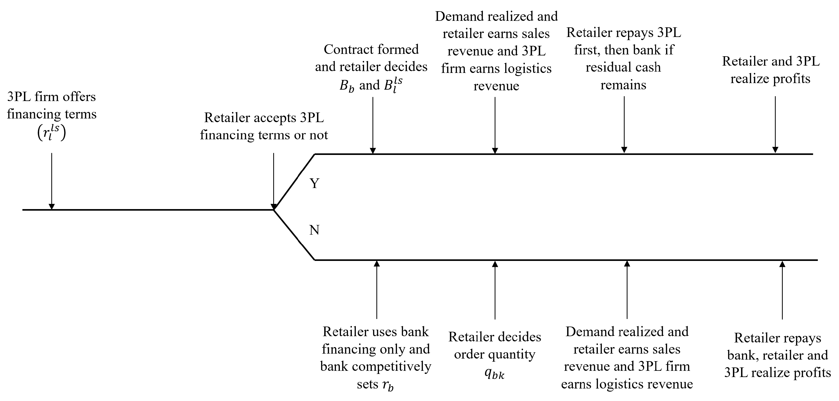j indexes the financing scenario, with $j=o,bk,dt,ls,bs$ denoting the benchmark case with sufficient internal capital, bank financing only, direct 3PL financing only, dual-channel financing with the 3PL firm as the senior creditor, and dual-channel financing with the bank as the senior creditor, respectively.

, and the event sequence is illustrated in Figure 1.

To facilitate tractable analysis, we follow Kouvelis and Zhao [2] and Yi et al. [68] by imposing the following standard technical assumptions. Both the retailer and the 3PL firm are risk-neutral and maximize their expected profits. Information is symmetric among all supply chain members. The risk-free interest rate is normalized to zero, that is, $r_f=0$. The opportunity cost of capital, or equivalently the time value of money, is also normalized to zero. Neither the bank nor the 3PL firm faces bankruptcy risk. The capital market is perfect, and the banking sector is perfectly competitive. We also consider a centralized supply chain in which a single decision maker has sufficient internal capital. The expected profit of the centralized supply chain is given by ${\pi }_c\left(q_c\right)=(p-c)\mathbb{E}\{min(q_c,\xi )\}-w_s{q}_c$, and the corresponding optimal order quantity is $q_c^{\ast }={\overline{F}}^{-1}\left({\displaystyle \frac{w_s}{p-c}}\right)$.

3.1. Retailer with Sufficient Internal Capital

We first consider the benchmark case in which the retailer has sufficient internal capital and therefore does not require external financing. In this case, the 3PL firm serves solely as a logistics service provider and delivers products to consumers when demand is realized. We use the superscript “o” to denote this benchmark scenario. We directly obtain the retailer’s optimal order quantity as

$$q_o^{\ast }={\overline{F}}^{-1}\left({\displaystyle \frac{w_s}{p-w_l}}\right),$$

(1)

For ease of exposition, we use $q_{un}={\overline{F}}^{-1}\left({\displaystyle \frac{w_s}{p-w_l}}\right)$ to denote the retailer’s optimal order quantity when internal capital is sufficient. Comparing $q_c^{\ast }={\overline{F}}^{-1}\left({\displaystyle \frac{w_s}{p-c}}\right)$ with $q_o^{\ast }={\overline{F}}^{-1}\left({\displaystyle \frac{w_s}{p-w_l}}\right)$ immediately yields $q_o^{\ast }\le q_c^{\ast }$. This inequality indicates that the introduction of the 3PL firm creates a double-marginalization effect in the supply chain, resulting in an equilibrium order quantity below that of the centralized system with sufficient capital.

3.2. Bank Financing as the Only Feasible Option

We next consider the case in which the retailer has no operating capital and bank financing is the only available funding source. We assume that the retailer borrows exactly $w_s{q}_{bk}$ from the bank, because borrowing is interest-bearing and the retailer has no alternative investment opportunity. We first derive the equilibrium bank interest rate $r_b$. Under the assumptions of a perfect financial market and competitively priced bank loans [4,40], the bank interest rate $r_b$ satisfies

$$w_s{q}_{bk}=\mathbb{E}\{min((p-w_l)min(q_{bk},\xi ),w_s{q}_{bk}(1+r_b))\},$$

(2)

The retailer’s expected profit is given by

$${\pi }_r^{bk}\left(q_{bk}\right)=\mathbb{E}{\{(p-w_l)min(q_{bk},\xi )-w_s{q}_{bk}(1+r_b)\}}^{+},$$

(3)

The retailer’s bankruptcy threshold under bank financing is ${\xi }_{bk}\left(q_{bk}\right)={\displaystyle \frac{w_s{q}_{bk}(1+r_b)}{p-w_l}}$. When $\xi \ge {\xi }_{bk}\left(q_{bk}\right)$, the retailer can fully repay the bank loan, namely $w_s{q}_{bk}(1+r_b)$. When $\xi <{\xi }_{bk}\left(q_{bk}\right)$, the retailer defaults, and the bank receives the retailer’s entire realized sales revenue, namely $(p-w_l)min(q_{bk},\xi )$.

Substituting Equation (2) into Equation (3), the retailer’s expected profit can be rewritten as

$${\pi }_r^{bk}\left(q_{bk}\right)=(p-w_l)\mathbb{E}\{min(q_{bk},\xi )\}-w_s{q}_{bk}=(p-w_l)S\left(q_{bk}\right)-w_s{q}_{bk},$$

(4)

The 3PL firm’s expected profit is

$${\pi }_l^{bk}\left(q_{bk}\right)=(w_l-c)\mathbb{E}\{min(q_{bk},\xi )\}=(w_l-c)S\left(q_{bk}\right).$$

(5)

Equation (4) directly implies that $arg{max}_{q_{bk}}{\pi }_r^{bk}\left(q_{bk}\right)=q_{un}$. In other words, $r_b$ is the equilibrium interest rate charged by the bank when the retailer’s optimal order quantity under bank financing coincides with the unconstrained order quantity $q_{un}$. This result implies that, when bank financing is the retailer’s only feasible funding source and bank loans are competitively priced, the capital-constrained retailer’s equilibrium operating decision is identical to that in the absence of financial constraints. This finding is consistent with the existing literature showing that a competitive banking market separates the retailer’s financing decision from its operational decision.

3.3. Direct Financing by the 3PL Firm as the Only Feasible Financing Mode

We now consider the case in which the retailer has no access to any funding source other than the 3PL firm, i.e., direct financing by the 3PL firm is the retailer’s only feasible financing channel. In this case, $B_l=w_s{q}_{dt}$ and $B_b=0$. We next derive the retailer’s optimal order quantity $q_{dt}^{\ast }$ and the optimal lending rate $r_l^{\ast }$ charged by the 3PL firm. Similar to Section 3.2, the retailer borrows exactly $w_s{q}_{dt}$, because it has no alternative investment opportunity and must repay the 3PL loan with interest. Following Equation (3), if the retailer orders $q_{dt}$ units, its expected profit is given by

$$\begin{array}{cc}\hfill {\pi }_r^{dt}\left(q_{dt}\right)=& \mathbb{E}{\left\{(p-w_l)min(q_{dt},\xi )-w_s{q}_{dt}(1+r_l)\right\}}^{+}\hfill \\ \hfill =& (p-w_l)\left[S\left(q_{dt}\right)-S\left({\xi }_{dt}\left(q_{dt}\right)\right)\right],\hfill \end{array}$$

(6)

where ${\xi }_{dt}\left(q_{dt}\right)={\displaystyle \frac{w_s{q}_{dt}(1+r_l)}{p-w_l}}$ denotes the retailer’s bankruptcy threshold under direct financing by the 3PL firm. Solving the retailer’s problem yields the following lemma.

Lemma 1.

Under direct financing by the 3PL firm as the only feasible financing mode, for any given lending rate $r_l$, the retailer’s optimal order quantity $q_{dt}\left(r_l\right)$ satisfies

(i). 

If $0\le r_l<{\displaystyle \frac{p-w_l}{w_s}}-1$, then $q_{dt}$ is determined by

$$(p-w_l)\overline{F}\left(q_{dt}\right)=w_s(1+r_l)\overline{F}\left({\xi }_{dt}\left(q_{dt}\right)\right).$$

If $r_l={\displaystyle \frac{p-w_l}{w_s}}-1$, then $q_{dt}=\breve{q}$, where $G\left(\breve{q}\right)=1$.

(ii). 

${\displaystyle \frac{d{q}_{dt}}{d{r}_l}}\le 0$, and $q_{dt}\ge \breve{q}$.

Lemma 1(i) partitions the retailer’s ordering decision into two regions according to the lending rate $r_l$ charged by the 3PL firm. When the lending rate is relatively low, i.e., $0\le r_l<{\displaystyle \frac{p-w_l}{w_s}}-1$, the retailer finds the financing offer attractive and borrows $w_s{q}_{dt}$ from the 3PL firm, where $q_{dt}$ is determined by

$$(p-w_l)\overline{F}\left(q_{dt}\right)=w_s(1+r_l)\overline{F}\left({\xi }_{dt}\left(q_{dt}\right)\right).$$

The economic intuition is that the retailer chooses $q_{dt}$ such that the expected marginal revenue from the last unit sold, $(p-w_l)\overline{F}\left(q_{dt}\right)$, equals the expected marginal borrowing cost, $w_s(1+r_l)\overline{F}\left({\xi }_{dt}\left(q_{dt}\right)\right)$. When the 3PL lending rate reaches its upper bound, i.e., $r_l={\displaystyle \frac{p-w_l}{w_s}}-1$, the retailer regards the loan as sufficiently expensive and reduces its order quantity to $\breve{q}$. Lemma 1(ii) further shows that the retailer’s optimal order quantity $q_{dt}$ decreases with $r_l$, which is intuitive because a higher lending rate raises the retailer’s financing cost.

Anticipating the retailer’s order quantity $q_{dt}$, the 3PL firm’s expected profit can be written as

$$\begin{array}{cc}\hfill {\pi }_l^{dt}(q_{dt},r_l)=& (w_l-c)\mathbb{E}\left\{min(q_{dt},\xi )\right\}+\mathbb{E}\left\{min\left((p-w_l)min(q_{dt},\xi ),w_s{q}_{dt}(1+r_l)\right)\right\}-w_s{q}_{dt}\hfill \\ \hfill =& (w_l-c)S\left(q_{dt}\right)+(p-w_l)S\left({\xi }_{dt}\left(q_{dt}\right)\right)-w_s{q}_{dt}.\hfill \end{array}$$

(7)

Under this financing mode, the 3PL firm’s expected profit consists of the logistics profit plus the repayment it receives from direct financing, net of the principal lent to the retailer. To facilitate the analysis, we introduce the following technical assumption.

Definition 1.

$$z\left(q_{dt}\right):={\displaystyle \frac{1-G\left({\xi }_{dt}\left(q_{dt}\right)\right)}{G\left({\xi }_{dt}\left(q_{dt}\right)\right)-G\left(q_{dt}\right)}},$$

where $q_{dt}$ satisfies

$$(p-w_l)\overline{F}\left(q_{dt}\right)=w_s(1+r_l)\overline{F}\left({\xi }_{dt}\left(q_{dt}\right)\right).$$

This assumption depends only on the demand distribution. It is satisfied by several commonly used distributions, including the uniform distribution on $\left[0,a\right]$ and the exponential distribution with parameter τ on $\left[0,+\infty \right)$ (Yi et al. [68]). The function $z\left(q_{dt}\right)$ has the following properties: (1) $z\left(q_{dt}\right)$ is increasing in $q_{dt}$; (2) when $q_{dt}=\breve{q}$, $z\left(q_{dt}\right)=-{\displaystyle \frac{1}{2}}$.

Corollary 1.

Under direct financing by the 3PL firm as the only feasible financing mode (i.e., $B_l=w_s{q}_{dt}$ and $B_b=0$),

(i). 

${\displaystyle \frac{d{\pi }_r^{dt}\left(q_{dt}\right)}{d{r}_l}}<0$.

(ii). 

The retailer’s maximum order quantity $q_{dt}^{max}$ is determined by

$$\overline{F}\left(q_{dt}^{max}\right)=\overline{F}\left(q_{un}\right)\overline{F}\left(\overline{F}\left(q_{un}\right)q_{dt}^{max}\right),$$

and satisfies $q_{dt}^{max}\ge q_{un}$ and ${\displaystyle \frac{d{q}_{dt}^{max}}{d{w}_s}}<0$.

Corollary 1 shows that the retailer’s expected profit ${\pi }_r^{dt}\left(q_{dt}\right)$ decreases with the 3PL lending rate $r_l$. The intuition is straightforward: as the financing rate increases, the retailer’s borrowing cost rises, thereby reducing its expected profit. Moreover, because $r_l\ge 0$, it is useful to consider the extreme case in which $r_l=0$. By Lemma 1, the retailer’s order quantity then reaches its maximum level, denoted by $q_{dt}^{max}$. In this case, $q_{dt}^{max}(r_l=0)$ is characterized by Corollary 1(ii). The corollary also implies that $q_{dt}^{max}\ge q_{un}$ and that $q_{dt}^{max}$ decreases with the procurement cost $w_s$.

We next solve for the optimal lending rate from the 3PL firm’s perspective. The assumption that the 3PL firm is the retailer’s only feasible funding source is crucial, because the 3PL firm does not need to account for competition from the bank when setting its financing terms. By Corollary 1, the 3PL firm’s lending-rate decision can be equivalently viewed as a decision over the order quantity it intends to induce. Therefore, the 3PL firm’s optimal lending rate can be represented in terms of the induced order quantity $q_{dt}$.

Proposition 1.

Under direct financing by the 3PL firm as the only feasible financing mode, the 3PL firm’s optimal decision is characterized as follows. There exists a procurement-cost threshold ${\tilde{w}}_s=(2w_l-p-c)\overline{F}\left(\breve{q}\right)$. If $2w_l>p+c$ and $0<w_s<{\tilde{w}}_s$, then $q_{dt}^{\ast }=q_{dt}^{opt}$, where $q_{dt}^{opt}$ satisfies

$${\displaystyle \frac{p-c}{p-w_l}}+{\displaystyle \frac{G\left({\xi }_{dt}\left(q_{dt}^{opt}\right)\right)-G\left(q_{dt}^{opt}\right)}{1-G\left({\xi }_{dt}\left(q_{dt}^{opt}\right)\right)}}-{\displaystyle \frac{w_s}{(p-w_l)\overline{F}\left(q_{dt}^{opt}\right)}}=0.$$

If $2w_l>p+c$ and ${\tilde{w}}_s\le w_s\le p-w_l$, or if $2w_l\le p+c$, then $q_{dt}^{\ast }=\breve{q}$.

Proposition 1 shows that the 3PL firm’s lending decision is critically affected by the procurement cost $w_s$. When $2w_l\le p+c$, i.e., when the logistics charge is relatively low, the 3PL firm’s marginal logistics profit is limited. In this case, further lowering the lending rate to induce a larger order quantity would increase financing losses that cannot be offset by the additional logistics revenue. As a result, the 3PL firm sets the lending rate at its upper bound,

$$r_l={\displaystyle \frac{p-w_l}{w_s}}-1,$$

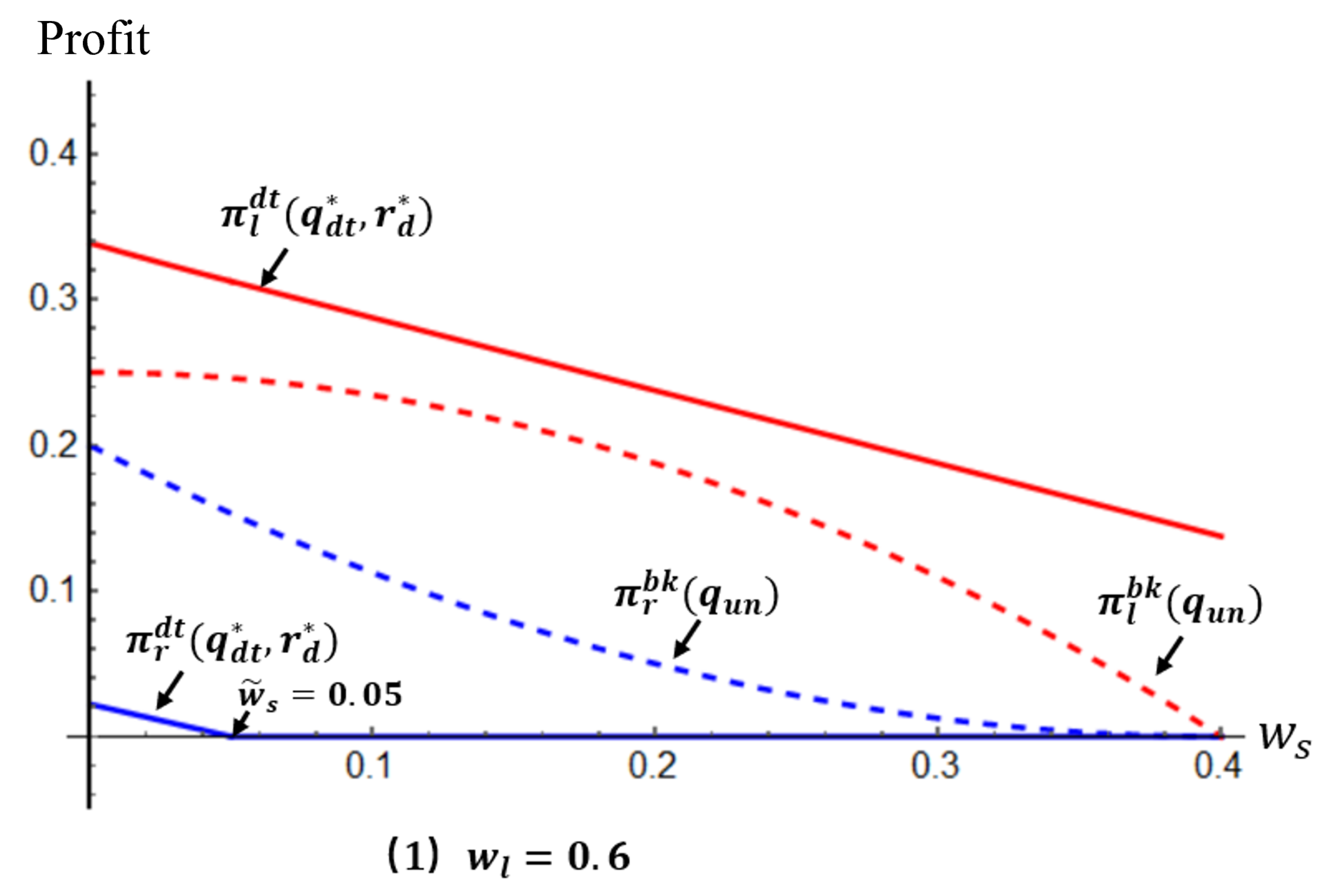
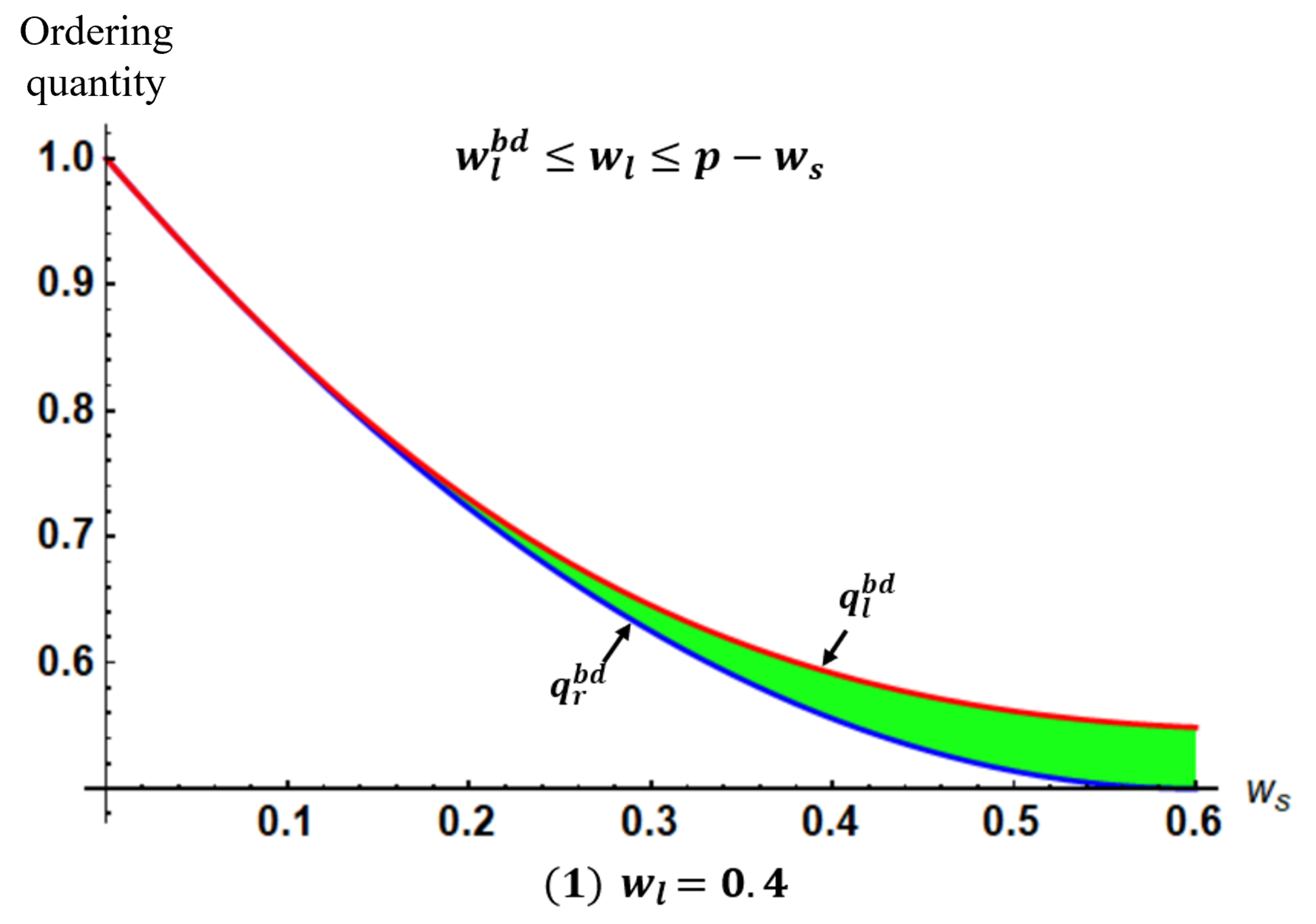
which implies $q_{dt}^{\ast }=\breve{q}$ and ${\pi }_r^{dt}(q_{dt}^{\ast },r_l^{\ast })=0$ (see Figure 2, where $2w_l-(p+c)=-0.1<0$). When $2w_l>p+c$, the 3PL firm enjoys a higher marginal logistics profit. However, if the procurement cost is sufficiently high, i.e., ${\tilde{w}}_s\le w_s\le p-w_l$, the retailer’s default risk becomes substantial. Even higher logistics revenue cannot compensate for the financing loss, and without an appropriate interest-rate adjustment the retailer may transfer excessive demand risk to the 3PL firm. Therefore, when the procurement cost is high, the 3PL firm again sets its lending rate at the upper bound, inducing $q_{dt}^{\ast }=\breve{q}$. By contrast, when $2w_l>p+c$ and the procurement cost is sufficiently low, i.e., $0<w_s<{\tilde{w}}_s$, the retailer’s default risk is relatively limited. 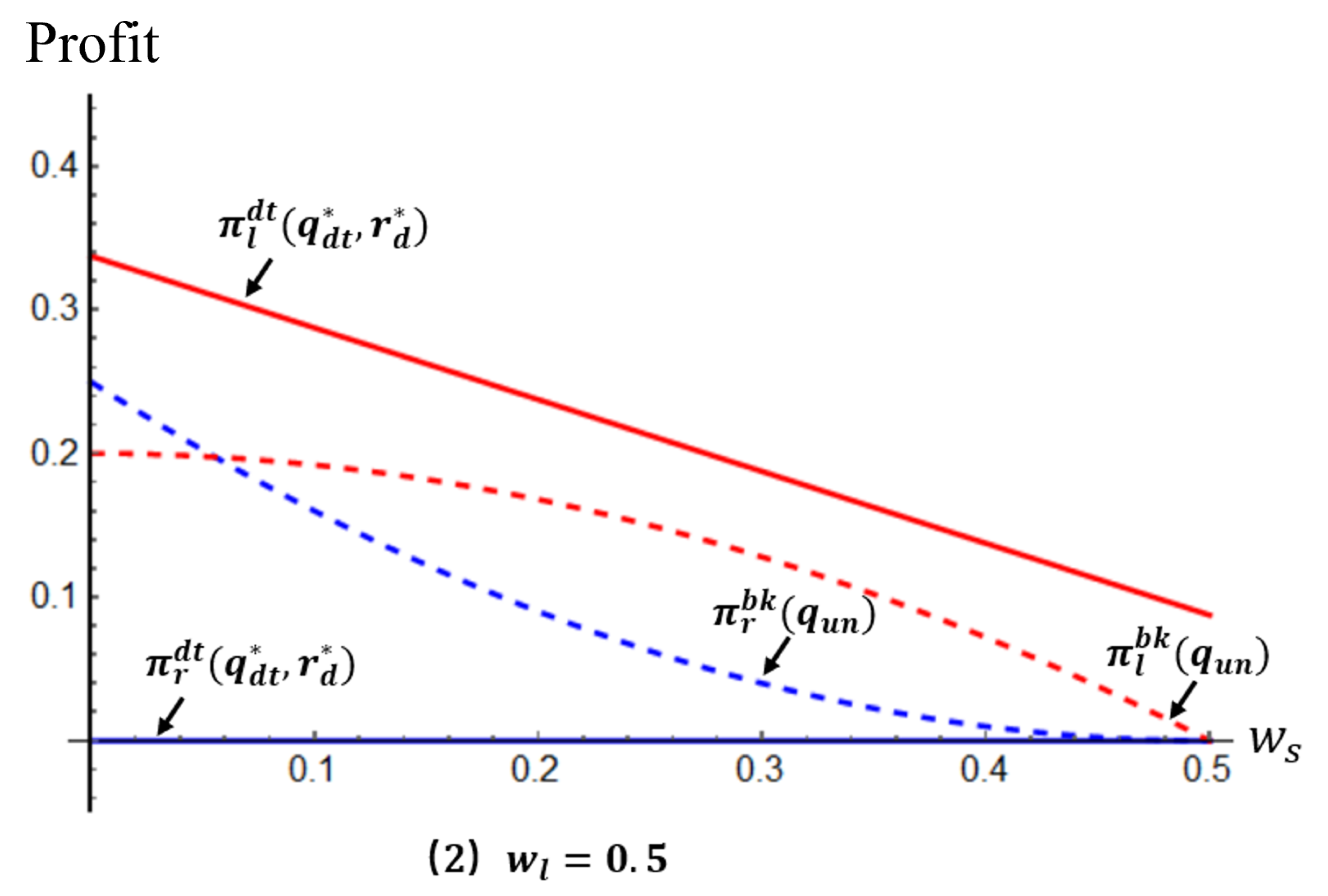In this region, the 3PL firm finds it more profitable to induce the order quantity $q_{dt}^{opt}$ (see Figure 3, where $2w_l-(p+c)=0.1>0$). For consistency across all figures, unless otherwise specified, we assume $p=1$, $c=0.1$, and that random demand follows a uniform distribution on $\left[0,1\right]$.

Corollary 2.

There exists $w_s^{\ast }=(p-c)\overline{F}\left(\breve{q}\right)$ such that, when $w_s=w_s^{\ast }$,

$${\pi }_c\left(w_s^{\ast }\right)={\pi }_l^{dt}\left(q_{dt}^{\ast }\left(w_s^{\ast }\right)\right).$$

Corollary 2 identifies a unique point at which direct financing by the 3PL firm coordinates the supply chain. This result suggests that, under the direct-financing-only regime, the 3PL firm can achieve the first-best outcome by absorbing part of the retailer’s demand risk, a feature that does not arise under bank financing. More generally, the coordination effect of direct 3PL financing is strongest when the procurement cost is at an intermediate level. When the procurement cost is low, the retailer retains substantial surplus, and the double-marginalization effect reduces total supply chain profit. When the procurement cost is high, financing risk borne by the 3PL firm becomes dominant, which is detrimental to both the 3PL firm and the supply chain as a whole. Compared with bank financing, this coordination effect also reveals the risk-sharing mechanism embedded in direct financing by the 3PL firm.

Previous studies have extensively examined alternative financing modes available to small and medium-sized enterprises facing capital constraints and have compared their performance. However, relatively little attention has been paid to situations in which a capital-constrained firm simultaneously adopts two or more financing sources. Therefore, when investigating inventory financing for the retailer, we next consider a dual-channel financing setting in which the retailer can simultaneously use direct financing from the 3PL firm and bank financing. We further assume that, when the retailer faces two creditors, the 3PL firm acts as the senior creditor, i.e., the retailer repays the 3PL loan before repaying the bank once sales revenue is realized. In this setting, several interesting questions arise: Will the retailer use both financing channels simultaneously, or choose only one of them? What are the equilibrium financing terms offered by the 3PL firm?

3.4. Dual-Channel Financing

We now consider a setting in which the retailer can simultaneously access bank financing and direct financing from the 3PL firm. Unless otherwise specified, we focus on the case in which the 3PL firm is the senior creditor. That is, once sales revenue is realized, the retailer repays the 3PL firm first and repays the bank only if residual cash remains. Acting as the Stackelberg leader, the 3PL firm first offers a financing contract characterized by the lending rate $r_l^{ls}$, where $r_l^{ls}$ denotes the interest rate charged by the 3PL firm under dual-channel financing when the 3PL firm has repayment priority. The contract is valid only if the retailer agrees to grant the 3PL firm senior creditor status. The retailer then determines the order quantity $q_{ls}$. Suppose that the retailer accepts the financing contract and borrows $B_l$ from the 3PL firm. If bank financing is also available, let $B_b$ denote the amount borrowed from the bank. The bank adjusts its loan rate $r_b^{ls}$ according to its junior-creditor status, as well as the amounts $B_l$ and $B_b$. Given the 3PL firm’s lending rate $r_l^{ls}$, the retailer’s expected profit is

$${\pi }_r^{ls}(q_{ls},B_l,B_b)=\mathbb{E}{\left\{(p-w_l)min(q_{ls},\xi )-B_l(1+r_l^{ls})-B_b(1+r_b^{ls})\right\}}^{+}.$$

(8)

Because the retailer borrows only the amount required to finance its order, the ordering decision satisfies

$$q_{ls}={\displaystyle \frac{B_l+B_b}{w_s}}.$$

From Equation (8), the retailer’s bankruptcy threshold with respect to the 3PL loan is

$${\xi }_l^{ls}={\displaystyle \frac{B_l(1+r_l^{ls})}{p-w_l}}.$$

If $\xi \ge {\xi }_l^{ls}$, the retailer can fully repay the 3PL firm, including both principal and interest, i.e., $B_l(1+r_l^{ls})$. Otherwise, the retailer defaults, and the 3PL firm receives the retailer’s entire sales revenue, namely $(p-w_l)min(q_{ls},\xi )$.

Similarly, the retailer’s bankruptcy threshold with respect to bank financing is defined as

$${\xi }_b^{ls}={\displaystyle \frac{B_l(1+r_l^{ls})+B_b(1+r_b^{ls})}{p-w_l}}={\xi }_l^{ls}+{\displaystyle \frac{B_b(1+r_b^{ls})}{p-w_l}}.$$

Since the 3PL firm is the senior creditor, it follows that ${\xi }_l^{ls}<{\xi }_b^{ls}$. If $\xi >{\xi }_b^{ls}$, i.e., when realized demand is sufficiently high, the retailer can fully repay both the 3PL firm and the bank. In that case, its realized profit is

$$(p-w_l)min(q_{ls},\xi )-B_l(1+r_l^{ls})-B_b(1+r_b^{ls});$$

otherwise, its realized profit is zero. In addition, the feasibility conditions $w_s(1+r_l^{ls})\le p-w_l$ and $w_s(1+r_b^{ls})\le p-w_l$ imply that

$$q_{ls}={\displaystyle \frac{B_l+B_b}{w_s}}={\displaystyle \frac{B_l}{w_s}}+{\displaystyle \frac{B_b}{w_s}}\ge {\displaystyle \frac{B_l(1+r_l^{ls})}{p-w_l}}+{\displaystyle \frac{B_b(1+r_b^{ls})}{p-w_l}}={\xi }_b^{ls}.$$

(9)

The 3PL firm’s expected profit is given by

$${\pi }_l^{ls}(q_{ls},B_l,B_b)=(w_l-c)\mathbb{E}\left\{min(q_{ls},\xi )\right\}+\mathbb{E}\left\{min\left((p-w_l)min(q_{ls},\xi ),B_l(1+r_l^{ls})\right)\right\}-B_l.$$

(10)

More specifically, if $\xi >{\xi }_l^{ls}$, the 3PL firm’s realized profit is $(w_l-c)min(q_{ls},\xi )+B_l{r}_l^{ls}$. If $\xi \le {\xi }_l^{ls}$, the retailer defaults and cannot fully repay the 3PL loan; in that case, the 3PL firm’s realized profit becomes $(p-c)min(q_{ls},\xi )-B_l$.

The bank’s lending rate $r_b^{ls}$ is determined by the following competitive-pricing condition:

$$B_b=\mathbb{E}\left\{min\left((p-w_l)min(q_{ls},\xi )-B_l(1+r_l^{ls}),B_b(1+r_b^{ls})\right)\right\}.$$

(11)

If ${\xi }_l^{ls}\le \xi \le {\xi }_b^{ls}$, the retailer’s sales revenue is sufficient to fully repay the 3PL firm but insufficient to fully repay the bank. If $\xi >{\xi }_b^{ls}$, the retailer can fully repay both creditors.

Lemma 2.

The bank interest rate $r_b^{ls}$ in Equation (11) has a nonnegative solution only if the bank loan amount satisfies $B_b<{\overline{B}}_b^{ls}$, where the upper bound ${\overline{B}}_b^{ls}$ is given by

$${\overline{B}}_b^{ls}=(p-w_l)\left[{\int }_0^{+\infty }\overline{F}\left(\xi \right)d\xi -{\int }_0^{{\xi }_l^{ls}}\overline{F}\left(\xi \right)d\xi \right].$$

(12)

Lemma 2 indicates that the amount the bank is willing to lend to the retailer is bounded above by the retailer’s expected sales revenue net of the amount promised to the 3PL firm. If the bank loan exceeds ${\overline{B}}_b^{ls}$, i.e., $B_b\ge {\overline{B}}_b^{ls}$, then the bank cannot break even in expectation.

The retailer chooses $(q_{ls},B_l,B_b)$ to maximize its expected profit ${\pi }_r^{ls}(q_{ls},B_l,B_b)$, subject to the upper bound on $B_b$. The 3PL firm chooses $r_l^{ls}$ to maximize its expected profit ${\pi }_l^{ls}(q_{ls},B_l,B_b)$. The retailer’s optimal response under dual-channel financing with the 3PL firm as the senior creditor is characterized in the following lemma.

Lemma 3.

Under dual-channel financing with the 3PL firm as the senior creditor, given the 3PL lending rate $r_l^{ls}$, the retailer’s optimal decision is characterized as follows:

(i). 

If $r_l^{ls}\ge r_b^{ls}$, the retailer chooses bank financing only, and the optimal decision is $(q_{ls},B_l,B_b)=(q_{un},0,w_s{q}_{un})$.

(ii). 

If $r_l^{ls}<r_b^{ls}$, the retailer chooses direct financing from the 3PL firm only, and the optimal decision is $(q_{ls},B_l,B_b)=(q_{ls},w_s{q}_{ls},0)$. In particular, when $r_l^{ls}={\displaystyle \frac{p-w_l}{w_s}}-1$, $q_{ls}=\breve{q}$; when $0\le r_l^{ls}<{\displaystyle \frac{p-w_l}{w_s}}-1$, $q_{ls}$ satisfies

$$(p-w_l)\overline{F}\left(q_{ls}\right)=w_s(1+r_l^{ls})\overline{F}\left({\displaystyle \frac{w_s{q}_{ls}(1+r_l^{ls})}{p-w_l}}\right).$$

Lemma 3 shows that if the 3PL firm’s lending rate is no lower than the bank’s rate, i.e., $r_l^{ls}\ge r_b^{ls}$, the retailer rejects the 3PL financing contract and relies exclusively on bank financing, where the bank interest rate is determined by Equation (2). If the 3PL firm’s lending rate is lower than the bank’s rate, i.e., $r_l^{ls}<r_b^{ls}$, the retailer chooses direct 3PL financing only, and the optimal decision follows from Lemma 1. Therefore, the retailer chooses either direct 3PL financing or bank financing, but never both simultaneously. The intuition is as follows. Suppose the retailer were to use both financing sources. If $r_l^{ls}<r_b^{ls}$, direct financing from the 3PL firm is cheaper, and the retailer would optimally switch entirely to 3PL financing to reduce borrowing costs. Conversely, if $r_l^{ls}\ge r_b^{ls}$, bank financing is cheaper. Moreover, the proof of Lemma 2 implies that, for a given order quantity, $r_b^{ls}$ decreases with $B_b$, i.e., the more the retailer borrows from the bank, the lower the bank’s interest rate. The retailer would then reduce borrowing from the 3PL firm and increase bank borrowing to further lower financing costs. Because the 3PL firm has senior creditor status, a smaller 3PL loan also implies a lower bank interest rate and a higher likelihood that the bank will be fully repaid. Taken together, when the 3PL firm is the senior creditor, simultaneously using bank financing and direct 3PL financing is never optimal for the retailer.

When the retailer uses only direct financing from the 3PL firm, the results in Corollary 1 continue to hold. Proposition 1 shows that, in the absence of bank financing as an alternative, the 3PL firm can induce the retailer to order $q_{dt}^{opt}$. However, if bank financing is also available, the 3PL firm must make direct financing sufficiently attractive relative to bank financing. In other words, the order quantity induced by the 3PL firm must ensure that the retailer’s expected profit under direct 3PL financing, ${\pi }_r^{ls}\left(q_{ls}\right)$, is no lower than its expected profit under bank financing, ${\pi }_r^{bk}\left(q_{un}\right)$. In addition, if the 3PL firm’s expected profit under direct financing, ${\pi }_l^{ls}\left(q_{ls}\right)$, is lower than its profit under bank financing, ${\pi }_l^{bk}\left(q_{un}\right)$, then the 3PL firm will not offer such a financing contract either.

Lemma 4.

Under dual-channel financing with the 3PL firm as the senior creditor,

(i). 

There exists a threshold $q_r^{bd}\in \left[\breve{q},q_{dt}^{max}\right]$ such that, when $q_{dt}\ge q_r^{bd}$, we have ${\pi }_r^{dt}\left(q_{dt}\right)\ge {\pi }_r^{bk}\left(q_{un}\right)$; when $q_{dt}\le q_r^{bd}$, we have ${\pi }_r^{dt}\left(q_{dt}\right)\le {\pi }_r^{bk}\left(q_{un}\right)$. Here,

$$q_r^{bd}=\left\{q_{dt}:{\pi }_r^{dt}\left(q_{dt}\right)={\pi }_r^{bk}\left(q_{un}\right)\right\}.$$

(ii). 

There exists a threshold $q_l^{bd}\in \left[q_{dt}^{opt},q_{dt}^{max}\right]$ such that, when $q_{dt}\in \left[q_{dt}^{opt},q_l^{bd}\right]$, we have ${\pi }_l^{dt}\left(q_{dt}\right)\ge {\pi }_l^{bk}\left(q_{un}\right)$; when $q_{dt}\in \left[q_l^{bd},q_{dt}^{max}\right]$, we have ${\pi }_l^{dt}\left(q_{dt}\right)\le {\pi }_l^{bk}\left(q_{un}\right)$. Here,

$$q_l^{bd}=\left\{q_{dt}:{\pi }_l^{dt}\left(q_{dt}\right)={\pi }_l^{bk}\left(q_{un}\right)\right\}.$$

We first clarify the economic meanings of the two thresholds in Lemma 4. The threshold $q_r^{bd}$ is the smallest order quantity induced by the 3PL firm that makes the retailer indifferent between direct 3PL financing and bank financing. The threshold $q_l^{bd}$ is the largest order quantity induced by the 3PL firm that makes the 3PL firm indifferent between these two financing modes. Since ${\pi }_r^{dt}\left(q_{dt}\right)$ increases with $q_{dt}$ (see Lemma 1 and Corollary 1), the retailer prefers direct 3PL financing whenever the induced order quantity exceeds $q_r^{bd}$; otherwise, bank financing is more attractive. Similarly, Proposition 1 implies that the 3PL firm’s expected profit ${\pi }_l^{dt}\left(q_{dt}\right)$ decreases with $q_{dt}$ over the interval $\left[q_{dt}^{opt},q_{dt}^{max}\right]$. Therefore, if the induced order quantity exceeds $q_l^{bd}$, the 3PL firm prefers the retailer to rely on bank financing instead. If the equation ${\pi }_l^{dt}\left(q_{dt}\right)={\pi }_l^{bk}\left(q_{un}\right)$ has no solution over $\left[q_{dt}^{opt},q_{dt}^{max}\right]$, then ${\pi }_l^{dt}\left(q_{dt}\right)\ge {\pi }_l^{bk}\left(q_{un}\right)$ holds throughout that interval. In this case, the maximum order quantity the 3PL firm is willing to induce is $q_{dt}^{max}$, attained when $r_l=0$.

Proposition 2.

Under dual-channel financing with the 3PL firm as the senior creditor, there exist a procurement-cost threshold

$$w_s^{bd}={\displaystyle \frac{4(w_l^2-c{w}_l-p{w}_l+pc)}{c-p}}$$

and a logistics-charge threshold

$$w_l^{bd}={\displaystyle \frac{1}{4}}(p+3c).$$

The equilibrium financing strategy of the 3PL firm is characterized as follows:

(i). 

If $c\le w_l\le w_l^{bd}$ and $w_s^{bd}\le w_s\le p-w_l$, the 3PL firm prefers the retailer to use bank financing.

(ii). 

If $c\le w_l\le w_l^{bd}$ and $0\le w_s\le w_s^{bd}$, or if $w_l^{bd}\le w_l\le p-w_s$, the order quantity induced by the 3PL firm is

$$q_{ls}^{opt}=max\left(q_r^{bd},q_{dt}^{opt}\right).$$

Equivalently, the 3PL firm’s optimal lending rate is either determined by

$$\overline{F}\left(q_{dt}^{opt}\right)={\displaystyle \frac{w_s(1+r_l)}{p-w_l}}\overline{F}\left({\displaystyle \frac{w_s(1+r_l)}{p-w_l}}{q}_{dt}^{opt}\right),$$

where $q_{dt}^{opt}$ satisfies

$${\displaystyle \frac{p-c}{p-w_l}}+{\displaystyle \frac{G\left({\xi }_{dt}\left(q_{dt}^{opt}\right)\right)-G\left(q_{dt}^{opt}\right)}{1-G\left({\xi }_{dt}\left(q_{dt}^{opt}\right)\right)}}-{\displaystyle \frac{w_s}{(p-w_l)\overline{F}\left(q_{dt}^{opt}\right)}}=0,$$

or by the interest rate corresponding to the threshold order quantity $q_r^{bd}$, at which the retailer is just indifferent between direct 3PL financing and bank financing.

Proposition 2 shows that when the logistics charge is low and the procurement cost is high, the 3PL firm prefers the retailer to rely on bank financing; by contrast, when both the logistics charge and procurement cost are low, or when the logistics charge is sufficiently high, the 3PL firm is willing to offer direct financing. The intuition is as follows. The 3PL firm’s expected profit consists of two components: revenue from logistics service and the gain or loss associated with financing. 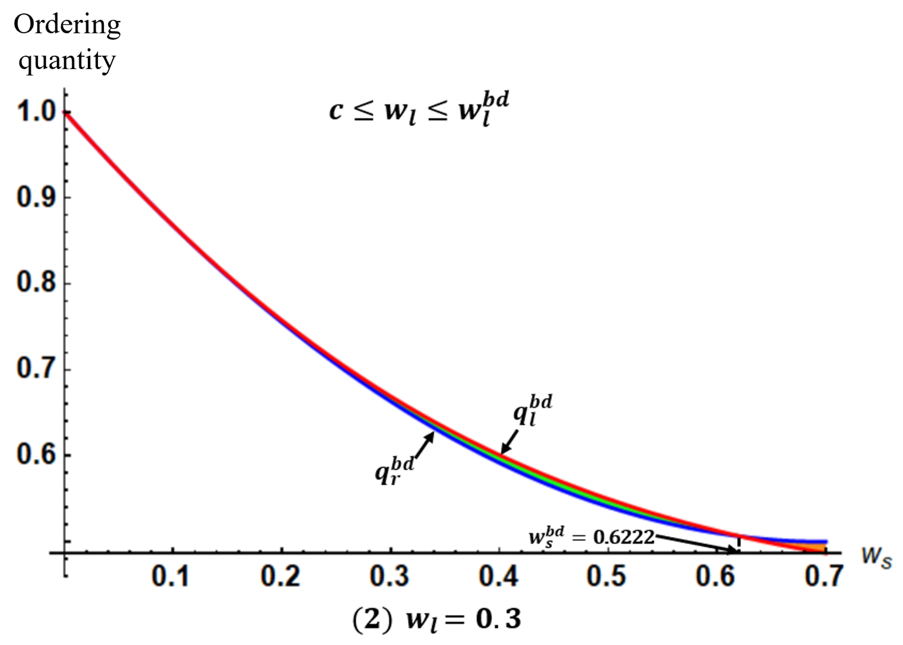When the logistics charge is low and the procurement cost is high ($c\le w_l\le w_l^{bd}$ and $w_s^{bd}\le w_s\le p-w_l$; see the orange region in Figure 4), the 3PL firm’s logistics revenue is limited, while the retailer’s default risk is high. As a result, the financing risk borne by the 3PL firm is substantial, and the relatively low logistics revenue is insufficient to offset the financial loss generated by financing. In this region, the 3PL firm’s expected profit is lower than that under bank financing. When both the logistics charge and the procurement cost are low ($c\le w_l\le w_l^{bd}$ and $0\le w_s\le w_s^{bd}$; see the green region in Figure 4), the 3PL firm’s logistics revenue remains relatively low, but the retailer’s default risk is also limited. In this case, the financing-related loss can be offset by logistics revenue, so direct financing becomes optimal for the 3PL firm. When the logistics charge is high ($w_l^{bd}\le w_l\le p-w_s$; see the green region in Figure 5), the 3PL firm’s logistics revenue is sufficiently large that the financing loss can be absorbed regardless of the procurement cost, and the 3PL firm therefore prefers to offer direct financing. In the latter two cases, the 3PL firm induces the retailer to order $q_{ls}^{opt}$, which is no smaller than either $q_{dt}^{opt}$, the optimal order quantity under direct-financing-only, or $q_r^{bd}$, the minimum order quantity required to make the retailer willing to choose direct 3PL financing over bank financing.

3.5. Equilibrium Structure and Boundary Conditions

The above results show that the equilibrium financing structure is driven by three mathematical forces. First, under the IFR demand assumption, the retailer’s expected profit under direct 3PL financing is concave in the relevant decision region, so the retailer’s best response can be uniquely characterized by the first-order condition in Lemma 1. Second, the bank’s competitive-pricing condition imposes an upper bound on feasible bank lending when the bank is the junior creditor. This feasible-lending boundary limits the retailer’s ability to combine bank financing with 3PL financing. Third, creditor priority changes the marginal cost of each financing source. When the 3PL firm is the senior creditor, any positive 3PL loan must be repaid before the bank loan, which worsens the bank’s repayment position and raises the bank’s required compensation. As a result, the retailer’s optimal borrowing structure is located at a boundary solution: either $B_l=0$ or $B_b=0$. This explains why mixed financing does not arise in the main model.

The boundary nature of the equilibrium should not be interpreted as a universal property of dual-channel financing. It depends on the repayment hierarchy and the competitive-pricing rule of the bank. When the bank is the senior creditor, the bank loan is protected by repayment priority, while the 3PL firm can still benefit from a larger order quantity through logistics revenue. Consequently, the marginal values of bank financing and 3PL financing are no longer ordered in the same way, and an interior mixed-financing region may emerge. This comparison also clarifies why creditor priority is a central structural determinant of the financing equilibrium.

4. Extensions

4.1. The Bank as the Senior Creditor

Suppose that the financing contract offered by the 3PL firm is characterized by the interest rate $r_l^{bs}$, i.e., the 3PL firm does not require senior creditor status. In this case, the retailer will naturally assign senior creditor status to the bank, as doing so is optimal from the retailer’s perspective. The reason is that, when the 3PL firm does not insist on repayment priority, granting such priority to the bank lowers the bank’s default threshold and thus reduces the bank’s lending rate, thereby increasing the retailer’s expected profit. Suppose that the retailer borrows $B_l$ from the 3PL firm and $B_b$ from the bank, and that the bank is the senior creditor. The expected profits of the retailer and the 3PL firm are then given by

$${\pi }_r^{bs}(q_{bs},B_l,B_b)=\mathbb{E}{\left\{(p-w_l)min(q_{bs},\xi )-B_b(1+r_b^{bs})-B_l(1+r_l^{bs})\right\}}^{+}$$

(13)

and

$$\begin{array}{cc}\hfill {\pi }_l^{bs}(q_{bs},B_l,B_b)& =(w_l-c)\mathbb{E}\left\{min(q_{bs},\xi )\right\}\hfill \\ \hfill & +\mathbb{E}\left\{min\left((p-w_l)min(q_{bs},\xi )-B_b(1+r_b^{bs}),B_l(1+r_l^{bs})\right)\right\}-B_l.\hfill \end{array}$$

(14)

The bank’s lending rate $r_b^{bs}$ is determined by the following competitive-pricing condition:

$$B_b=\mathbb{E}\left\{min\left((p-w_l)min(q_{bs},\xi ),B_b(1+r_b^{bs})\right)\right\}.$$

(15)

Because the retailer borrows only the amount necessary to finance its order, the corresponding order quantity is

$$q_{bs}={\displaystyle \frac{B_l+B_b}{w_s}}.$$

Define the retailer’s bankruptcy threshold with respect to bank financing as

$${\xi }_b^{bs}={\displaystyle \frac{B_b(1+r_b^{bs})}{p-w_l}}.$$

Similarly, define the bankruptcy threshold with respect to direct financing by the 3PL firm as

$${\xi }_d^{bs}={\xi }_b^{bs}+{\displaystyle \frac{B_l(1+r_l^{bs})}{p-w_l}}.$$

Since the bank is the senior creditor, we have ${\xi }_b^{bs}<{\xi }_d^{bs}$. In addition, it holds that $q_{bs}\ge {\xi }_d^{bs}$. Similar to Equation (12), Equation (15) admits a nonnegative solution for $r_b^{bs}$ as long as $B_b<{\overline{B}}_b^{bs}$, where

$${\overline{B}}_b^{bs}=(p-w_l){\int }_0^{+\infty }\overline{F}\left(\xi \right)d\xi .$$

Notably, under dual-channel financing with the bank as the senior creditor, the bank’s lending limit ${\overline{B}}_b^{bs}$ equals the retailer’s total expected revenue net of logistics charges payable to the 3PL firm (the proof is omitted for brevity). The retailer chooses $(q_{bs},B_l,B_b)$ to maximize its expected profit ${\pi }_r^{bs}(q_{bs},B_l,B_b)$, subject to the upper bound ${\overline{B}}_b^{bs}$ on $B_b$. The 3PL firm chooses $r_l^{bs}$ to maximize its expected profit ${\pi }_l^{bs}(q_{bs},B_l,B_b)$.

Lemma 5.

Under dual-channel financing with the bank as the senior creditor, given the 3PL firm’s lending rate $r_l^{bs}$, there exists an interest-rate threshold $r_{db}$ satisfying

$${\displaystyle \frac{1}{\overline{F}\left({\xi }_b^{bs}\right)}}=1+r_{db},$$

where ${\xi }_b^{bs}$ is determined by

$$(p-w_l){\int }_0^{{\xi }_b^{bs}}\overline{F}\left(\xi \right)d\xi =w_s{q}_{un}.$$

The retailer’s optimal decision is characterized as follows:

(i). 

If $r_l^{bs}=0$, then $B_b^{\ast }=0$, and $B_l^{\ast }$ satisfies

$$\overline{F}\left({\displaystyle \frac{B_l^{\ast }}{w_s}}\right)={\displaystyle \frac{w_s}{p-w_l}}\overline{F}\left({\displaystyle \frac{B_l^{\ast }}{p-w_l}}\right).$$

(ii). 

If $0<r_l^{bs}\le r_{db}$, then $B_l^{\ast }$ and $B_b^{\ast }$ are jointly determined by

$$B_b^{\ast }=(p-w_l){\int }_0^{{\overline{F}}^{-1}\left({\displaystyle \frac{1}{1+r_l^{bs}}}\right)}\overline{F}\left(\xi \right)d\xi$$

(16)

and

$$\overline{F}\left({\displaystyle \frac{B_l^{\ast }+B_b^{\ast }}{w_s}}\right)={\displaystyle \frac{w_s(1+r_l^{bs})}{p-w_l}}\overline{F}\left({\displaystyle \frac{B_l^{\ast }(1+r_l^{bs})}{p-w_l}}+{\overline{F}}^{-1}\left({\displaystyle \frac{1}{1+r_l^{bs}}}\right)\right),$$

(17)

with $r_b^{bs}\le r_l^{bs}$ and $B_b^{\ast }\le w_s{q}_{un}$.

(iii). 

If $r_l^{bs}>r_{db}$, then $B_l^{\ast }=0$ and $B_b^{\ast }=w_s{q}_{un}$.

Lemma 5 shows that the retailer’s financing choice and ordering decision depend critically on the 3PL firm’s lending rate $r_l^{bs}$. When $r_l^{bs}=0$, the retailer relies exclusively on direct 3PL financing. When $0<r_l^{bs}\le r_{db}$, the retailer simultaneously uses bank financing and direct 3PL financing. When $r_l^{bs}>r_{db}$, the retailer switches to bank financing only. The conclusions in Lemma 5(i) and Lemma 5(iii) are relatively straightforward. We therefore focus on the intuition behind Lemma 5(ii). Recall from Section 3.2 that when $q_{bk}>q_{un}$, the retailer’s expected profit ${\pi }_r^{bk}\left(q_{bk}\right)$ decreases with $q_{bk}$; hence, as long as the order quantity does not exceed $q_{un}$, bank financing remains relatively inexpensive. However, as a junior creditor, the 3PL firm may in some cases be willing to offer a sufficiently low rate to induce the retailer to order more than $q_{un}$. The reason is that, as the retailer’s logistics service provider, the 3PL firm can partially offset the cost of financing through logistics revenue and thereby earn a higher expected profit. Therefore, by simultaneously using bank financing and direct 3PL financing, the retailer can benefit both from transferring more demand risk to the 3PL firm and from ordering a larger quantity. This does not arise when the 3PL firm has senior creditor status, because the bank, unlike the 3PL firm, cannot recover part of the financing cost through logistics revenue and therefore has no incentive to lower its interest rate to induce joint borrowing. This extension serves as a sensitivity analysis of the creditor-priority assumption. The contrast between Lemma 3 and Lemma 5 shows that the no-mixing result in the main model is creditor-priority-dependent. When the 3PL firm is the senior creditor, mixed financing is dominated by a boundary financing structure. When the bank is the senior creditor, however, bank borrowing is less exposed to default risk, and the 3PL firm may still be willing to provide financing because a larger order quantity increases its logistics revenue. Hence, mixed financing can arise once the repayment hierarchy is changed.

4.2. Optimal Logistics Charge and Financing Terms

We next examine how the optimal logistics charge affects the financing contract.

Proposition 3.

When the 3PL firm simultaneously chooses the logistics charge and the lending rate, its optimal financing contract $(w_l^{\ast },r_l^{\ast })$ satisfies $r_l^{\ast }=0$.

Proposition 3 shows that when the 3PL firm is free to determine the logistics charge for each retailer, it is always optimal for the 3PL firm to offer zero-interest direct financing, under which the retailer relies exclusively on 3PL financing. The underlying intuition is as follows. When the retailer uses direct 3PL financing to fund its inventory, its optimal order quantity depends on the ratio ${\displaystyle \frac{w_s(1+r_l)}{p-w_l}}$, which implies that the effects of $w_l$ and $r_l$ on the retailer’s ordering decision are not independent. Therefore, the 3PL firm can increase its expected profit by raising $w_l$ while correspondingly lowering $r_l$ so as to keep ${\displaystyle \frac{w_s(1+r_l)}{p-w_l}}$ unchanged, until the lending rate reaches zero. Since the retailer will always prefer this zero-interest direct financing, $r_l^{\ast }=0$ is optimal, and bank financing under competitive pricing is no longer attractive.

This result is also consistent with Yi et al. [68], who show that when an intermediary platform charges a sufficiently high per-unit commission, it has an incentive to reduce the financing rate, potentially even below its opportunity cost of capital, in order to encourage farmers to expand production. The additional operating profit generated by the higher commission offsets the financing loss associated with the lower interest rate, ultimately benefiting the intermediary platform. A similar insight is reported by Deng et al. [25], who show that in buyer-financing settings, when the assembler can simultaneously choose the interest rate and the component procurement price, it should charge the lowest possible interest rate. Although the assembler may earn negative interest on financing extended to the supplier, it benefits more from the resulting increase in inventory and the lower procurement price of components.

Summary of key thresholds and equilibrium financing outcomes are summarized in

Table 2. Summary of key thresholds and equilibrium financing outcomes.

Condition	Financing Outcome	Decision
Bank financing only	Bank financing	$q^{bk}=q^{un}$
3PL financing only: $2w_l>p+c$, $0<w_s<{\tilde{w}}_s$	3PL direct financing	$q^{dt}=q_{dt}^{opt}$
3PL financing only: $2w_l\le p+c$ or ${\tilde{w}}_s\le w_s\le p-w_l$	3PL direct financing	$q^{dt}=\breve{q}$
3PL senior: $c\le w_l\le w_l^{bd}$, $w_s^{bd}\le w_s\le p-w_l$	Bank financing	$q^{ls}=q^{un}$
3PL senior: $c\le w_l\le w_l^{bd}$, $0\le w_s\le w_s^{bd}$	3PL direct financing	$q^{ls}=max\{q_r^{bd},q_{dt}^{opt}\}$
3PL senior: $w_l^{bd}\le w_l\le p-w_s$	3PL direct financing	$q^{ls}=max\{q_r^{bd},q_{dt}^{opt}\}$
Bank senior: $r_l^{bs}=0$	3PL direct financing only	$B_b^{\ast }=0,B_l^{\ast }>0$
Bank senior: $0<r_l^{bs}\le r^{db}$	Dual-channel financing	$B_b^{\ast }>0,B_l^{\ast }>0$
Bank senior: $r_l^{bs}>r^{db}$	Bank financing only	$B_b^{\ast }=w_s{q}^{un},B_l^{\ast }=0$
Endogenous logistics charge	3PL direct financing	$r_l^{\ast }=0$

.

5. Conclusions

This manuscript investigates the financing preferences of a capital-constrained retailer and a 3PL firm, as well as the conditions under which a financing contract can be reached between them, in a supply chain consisting of a capital-constrained retailer, a 3PL firm, and a bank. The analysis is conducted under a dual-channel financing setting in which the retailer can access both direct financing from the 3PL firm and bank financing. In addition, the manuscript derives the optimal ordering and financing decisions of the supply chain members once a financing contract is established. Several important findings and managerial implications emerge.

First, this manuscript analyzes the optimal decisions of the retailer and the 3PL firm under bank-financing-only and direct-3PL-financing-only settings. Under bank financing only, the retailer’s equilibrium order quantity is identical to that in the benchmark case without capital constraints. This result indicates that when the financial market is perfect and bank loans are competitively priced, the bank effectively serves as a funding pool for the capital-constrained retailer, so that capital constraints do not distort the retailer’s ordering decision. Nevertheless, due to the presence of the 3PL firm, the double-marginalization effect reduces the equilibrium order quantity relative to that in a centralized supply chain with sufficient capital, thereby lowering overall supply chain efficiency. This suggests that, in practice, vertical integration mechanisms such as mergers or acquisitions may help mitigate the inefficiency caused by double marginalization. Under direct financing by the 3PL firm only, the equilibrium order quantity and lending rate of the retailer and the 3PL firm are characterized. The analysis further identifies the procurement-cost condition under which direct 3PL financing can coordinate the supply chain. This result highlights the risk-sharing mechanism embedded in direct 3PL financing: by providing financing to the retailer, the 3PL firm absorbs part of the retailer’s demand uncertainty, which increases the retailer’s order quantity and improves supply chain coordination.

Second, under dual-channel financing with the 3PL firm as the senior creditor, the retailer never simultaneously uses both bank financing and direct 3PL financing. Instead, it chooses either bank financing only or direct 3PL financing only. From the 3PL firm’s perspective, when the logistics charge is low and the procurement cost is high, the 3PL firm prefers the retailer to rely on bank financing. By contrast, when the logistics charge is high, or when both the logistics charge and the procurement cost are low, the 3PL firm is willing to offer a financing contract and sets the optimal lending rate that makes the retailer willing to accept direct financing. These findings provide theoretical guidance for how a capital-constrained retailer should choose its financing source and determine its optimal order quantity under dual-channel financing.

Finally, the extension with the bank as the senior creditor shows that the retailer may optimally use both bank financing and direct 3PL financing simultaneously. This sharply contrasts with the case in which the 3PL firm is the senior creditor, and it demonstrates that creditor priority plays a crucial role in shaping the financing choice of a capital-constrained retailer. Therefore, creditor seniority should be explicitly incorporated into financing decisions under dual-channel financing. This manuscript also considers endogenous logistics pricing, where the 3PL firm simultaneously determines the logistics charge and the lending rate. The analysis shows that the 3PL firm’s optimal lending rate is zero. In other words, a 3PL firm with pricing power over logistics services always offers zero-interest direct financing, under which the retailer always prefers direct 3PL financing. This result also provides a theoretical explanation for the practice that supply chain firms may offer financing to capital-constrained firms at an interest rate no higher than the bank’s risk-free benchmark.

The applicability of the above findings should be understood within several boundary conditions. First, the equilibrium characterization relies on risk neutrality. If the retailer is risk averse, it may place greater weight on downside repayment risk and become less willing to expand orders through direct 3PL financing. This may shrink the region in which 3PL direct financing dominates bank financing. Second, the analysis assumes symmetric information. In practice, because the 3PL firm observes logistics flows and operational activities more closely than the bank, asymmetric information may strengthen the 3PL firm’s screening advantage and alter the bank’s competitive-pricing condition. Third, the baseline no-mixing result depends on the 3PL firm being the senior creditor and on the bank being competitively priced. As shown in the bank-seniority extension, changing the repayment hierarchy may restore mixed financing. Therefore, the no-mixing result should be interpreted as a creditor-priority-dependent equilibrium property rather than a universal prediction. Finally, this study is analytical and does not provide direct empirical validation. Future research may use transaction-level logistics and financing data, case evidence from 3PL financing platforms, or calibrated simulation analysis to examine the empirical relevance of the predicted financing regions.