Goal-Induced Pareto Fronts for a Bi-Criterion Truck–Multiple-Drone Routing Problem

Abstract

Truck–multiple-drone routing problems involve conflicting operational criteria and are therefore naturally suited to multiobjective analysis. In practical settings, however, decision makers may also specify aspiration levels for the considered criteria, which call for a target-oriented perspective. This paper studies a bi-criterion truck–multiple-drone routing problem through a goal-induced deviation framework in which the original objectives are transformed to normalized positive deviations with respect to prescribed targets. First, a general mathematical framework is introduced, and several structural properties are established, including dominance preservation, invariance under positive weighting, equivalence with the original Pareto structure when all the targets are violated, and the loss of discrimination when the targets are attainable. To address this latter effect, an enhanced goal-programming scalarization is proposed and shown to preserve consistency with the Pareto efficiency. The framework is then specialized to a truck–multiple-drone routing problem with truck time and makespan as criteria and evaluated on representative benchmark instances together with a broader attainable-target benchmark battery, using a common agent-based metaheuristic search framework adapted from literature. This search framework is employed both to estimate a reference Pareto frontier and to solve the GP and EGP scalarizations under the same computational scheme. The computational results illustrate two target regimes: When the targets are unattainable, both formulations are mainly driven by the minimization of positive deviations; when they are attainable, classical goal programming may return satisfactory but dominated solutions, whereas the enhanced formulation preserves discrimination and selects Pareto-efficient alternatives.

1. Introduction

The rapid growth of e-commerce and the increasing pressure to provide faster, more flexible, and more sustainable last-mile delivery services have fostered the development of hybrid logistics systems integrating trucks and unmanned aerial vehicles. Within this context, truck–drone routing problems have emerged as a highly active research field since they offer the possibility of combining the endurance and carrying capacity of ground vehicles with the agility and speed of aerial resources. As these systems become more realistic, however, their operational design also becomes substantially more difficult, particularly when multiple drones, synchronization requirements, multi-visit missions, and flexible rendezvous decisions must be jointly considered [1,2,3,4].

Among the different variants proposed in the literature, the truck–multiple-drone setting has attracted growing attention because of its closer connection to real operational environments. In such systems, several drones may cooperate with a truck to serve customers under complex launch, recovery, waiting, and synchronization patterns. These decisions typically create tradeoffs between service quality and resource consumption. In particular, reducing the overall completion time may require a more intensive use of the truck or more aggressive synchronization policies, whereas reducing truck usage may deteriorate the makespan or restrict the exploitation of drone capabilities. This conflict between efficiency criteria naturally motivates a multiobjective optimization perspective [5,6,7].

Recent research has already shown the value of Pareto-based approaches for these problems. In particular, our previous work on the truck–multidrone traveling problem with launch operations and flexible rendezvous points approached the routing problem from a bi-objective perspective in which customer service performance and truck usage were optimized simultaneously, thus providing the decision maker with an estimated Pareto front of high-quality tradeoff solutions. That study emphasized that beyond the sole minimization of the service completion time, practical implementations increasingly require incorporating an additional criterion linked to the environmental and operational impacts of truck movement and that a spread set of non-dominated solutions may offer useful support for managerial decision making [7].

Nevertheless, Pareto front approximation alone does not fully exploit situations in which the decision maker can specify explicit aspiration levels for the performance criteria under consideration. In many realistic logistics settings, practitioners are interested not only in obtaining a generic set of efficient solutions but also in evaluating such solutions relative to target values that reflect service agreements, sustainability commitments, or internal operational benchmarks. In such cases, goal programming (GP) provides a natural decision analytic framework since it measures the extent to which predefined aspiration levels are achieved or violated [8,9,10,11,12].

A particularly relevant feature of GP for the present work is that for goals of the form $f_i\left(x\right)\le g_i$, the problem can be reformulated as the minimization of positive deviations from fixed aspiration levels. Dhouib et al. explicitly exploit this idea by converting a GP model to a multiobjective optimization problem that minimizes deviations from the goals and then solving the resulting problem through a hybrid metaheuristic designed to approximate a Pareto set of solutions in a single run [13]. This conversion is especially appealing in complex nonlinear or combinatorial environments, where directly solving the original GP model may be impractical.

Motivated by these observations, this paper proposes a goal-programming-oriented extension of the bi-criterion truck–multiple-drone routing framework. Rather than working only with the original objective space, we introduce a goal-induced deviation space in which each criterion is transformed to a normalized positive deviation with respect to a target level. This transformation preserves the decision-making meaning of aspiration levels while keeping the problem within a multiobjective setting. The resulting representation makes it possible to analyze not only the classical Pareto front associated with the original routing criteria but also a goal-induced Pareto front describing efficient tradeoffs in terms of target nonachievement.

The contribution of the paper is twofold. First, a general mathematical framework is introduced for multiobjective minimization problems with aspiration levels, and several structural properties of the induced deviation-based Pareto front are established. In particular, the paper studies the effects of normalization and positive weighting, as well as the relationship between the original Pareto front and the goal-induced one. Second, this framework is specialized to a bi-criterion truck–multiple-drone routing problem in which the criteria are related to service performance and truck usage. For the computational study, the paper employs a common agent-based metaheuristic search framework adapted from León-Blanco et al. [4]. This search engine is used to estimate a reference Pareto frontier in the original objective space and to solve both the classical GP and the enhanced GP scalarizations under the same computational scheme. Accordingly, the computational analysis is aimed at assessing the effect of the proposed enhanced goal-programming formulation relative to classical GP rather than at benchmarking general-purpose multiobjective metaheuristics. In this way, the paper bridges multiobjective routing, goal programming, and decision-oriented analysis for coordinated truck–multiple-drone logistics.

From an application viewpoint, the proposed approach offers a richer decision-support perspective than a purely Pareto-based analysis. The original efficient frontier describes the operational tradeoffs inherent to the routing problem, whereas the goal-induced frontier reflects how those tradeoffs are perceived once explicit managerial targets are introduced. This distinction is relevant because aspiration levels may compress or reshape the efficient set in a nontrivial manner, highlighting solutions that are particularly well aligned with practical preferences. Hence, beyond algorithmic performance, the paper also aims to clarify how target values influence the structures of efficient solutions in truck–multiple-drone operations.

The remainder of the paper is organized as follows. Section 2 reviews the related literature on truck–multiple-drone routing, multiobjective optimization, and goal programming. Section 3 presents the general deviation-based framework, develops the main theoretical results, introduces an illustrative theoretical case, and specializes the model to the bi-criterion truck–multiple-drone setting together with the adopted solution methodology. Section 4 reports and discusses the numerical results. Finally, Section 5 summarizes the main conclusions and outlines future research directions.

2. Literature Review

2.1. Truck–Drone and Truck–Multiple-Drone Routing Problems

The study of coordinated truck–drone delivery systems has its origins in the Flying Sidekick Traveling Salesman Problem introduced by Murray and Chu, where a truck and a drone cooperate in parcel distribution under synchronization constraints [1]. Since then, the literature has evolved toward more realistic and operationally relevant settings, including multiple drones, heterogeneous fleets, battery-related restrictions, flexible launch and recovery decisions, and richer routing structures [2]. This evolution reflects the need to better capture the complexities of modern last-mile logistics, where hybrid ground–air delivery systems are increasingly viewed as a promising alternative for combining service efficiency with operational flexibility.

A particularly important stream within this literature concerns the use of multiple drones in cooperation with a single truck. In such settings, the truck may act not only as a mobile depot but also as an active delivery vehicle, while drones may perform one or several visits between synchronization points. This richer class of problems significantly enlarges the decision space since routing, assignment, timing, and rendezvous decisions become strongly interdependent. For example, Luo et al. studied a multiple-drone setting with repeated aerial use, whereas Gu et al. proposed a hybrid algorithm for a vehicle routing problem with drones and multiple visits [14,15]. However, much of this literature remains focused on single-objective optimization or on weighted aggregations of different cost components.

In parallel, other contributions have emphasized more general collaborative truck–multidrone systems in which both the truck and the drones may serve customers and in which rendezvous locations need not coincide with launch positions. In this line, Gonzalez-R. et al. proposed a heuristic framework for multi-drop truck–drone route planning [3], and León-Blanco et al. introduced the Truck–Multidrone Team Logistics Problem (TmDTL), addressing large-scale instances through a multi-agent perspective under a single objective, namely, makespan minimization [4]. These studies are particularly relevant because they move closer to realistic operational environments, where synchronization and resource coordination are central to solution quality.

Building on this stream, our previous work addressed the TmDTL from a bi-criterion perspective by jointly minimizing the total service time and truck usage, thereby providing the decision maker with an estimated Pareto front of routing alternatives [7]. That work highlighted two important aspects. First, truck–multiple-drone delivery should not be evaluated exclusively through service speed since truck usage also captures relevant economic and environmental effects. Second, in this class of problems, the decision maker may benefit from an a posteriori multiobjective approach in which a spread set of non-dominated solutions is generated before the final routing alternative is selected. These observations motivate the present study, which preserves the multiobjective nature of the problem while incorporating explicit aspiration levels for the considered criteria.

2.2. Multiobjective Approaches in Routing Problems

Multiobjective optimization has long been recognized as a suitable framework for routing problems involving competing criteria, such as cost, time, environmental impact, service quality, or resource utilization. In contrast to single-objective formulations based on weighted sums, Pareto-based approaches aim to approximate a set of efficient tradeoff solutions, thus avoiding the premature fixation of a unique preference structure and providing the decision maker with a richer view of the feasible compromises [6,16,17].

In truck–drone logistics, this perspective is especially appropriate because the operational criteria are frequently conflicting. Reducing the completion time may require a more intensive use of the truck, more synchronization events, or more aggressive exploitation of drone resources. Conversely, reducing the truck mileage or truck operating time may constrain the routing structure and increase the overall service duration. Some studies have incorporated multiple criteria through weighted combinations, which can be effective when preferences are precisely known in advance. However, such approaches typically produce a single solution for each weight configuration and may fail to describe the overall geometry of the tradeoff surface [5,15].

Pareto-based methodologies are, therefore, attractive when the decision maker prefers an a posteriori process. In our previous bi-criterion TmDTL work, this standpoint was explicitly adopted, and the proposed algorithm was designed to estimate high-quality Pareto fronts in a reasonable computational time [7]. The resulting set of non-dominated solutions enabled the decision maker to compare different balances between the makespan and truck usage, which, in turn, translated to different service and sustainability profiles. This idea is consistent with broader discussions in multiobjective routing, where the quality of a method is measured not only by the best scalarized value found but also by its ability to provide a diverse and representative efficient frontier [6,18].

Despite these advances, Pareto front approximation does not, by itself, incorporate explicit target values for the criteria. In practice, decision makers may wish to specify aspiration levels, such as the maximum acceptable completion time or a desired upper bound on truck usage. Once such target values are introduced, the interpretation of the efficiency changes: The relevant question is no longer only how solutions trade one objective against another but also how they behave relative to those target levels. This observation suggests that a deviation-based perspective, rooted in goal programming, may complement and enrich the standard Pareto analysis.

2.3. Goal Programming and Deviation-Based Reformulations

Goal programming is one of the classical approaches for dealing with multiple criteria in decision-making problems. Its central idea is to assign aspiration levels to the criteria and then minimize the deviations between the achieved values and the desired targets [8,9,10,11,19]. Over time, both weighted and lexicographic variants of GP have been extensively studied, and the approach has been applied in numerous managerial and engineering contexts [12,20].

For minimization-type goals of the form $f_i\left(x\right)\le T_i$, GP naturally leads to the minimization of positive deviations above the aspiration levels. This property is especially useful in combinatorial and nonlinear problems because it permits interpreting target nonachievement as a new performance criterion. In fact, Dhouib et al. explicitly exploit this idea by converting a GP model to a multiobjective optimization problem which components are the deviations from the target levels and then solving the resulting problem with a hybrid metaheuristic aimed at approximating the corresponding Pareto set [13]. Their work is particularly relevant for the present paper because it shows that rather than scalarizing all the preferences from the beginning, one may keep a multiobjective structure in the deviation space and search for non-dominated deviation profiles.

More recently, goal-programming-based methodologies have also been used in application domains where sensitivity to weights and target values is important. For instance, Mallidis et al. proposed a goal-programming framework for machine-learning model selection, emphasizing that the method allows the analyst to examine the impacts of both significance weights and threshold values in a computationally efficient way [21]. Although the application domain is very different from vehicle routing, the methodological lesson is important: Target levels do not merely shift objective values but may alter the interpretation of what constitutes a desirable or balanced solution.

However, to the best of our knowledge, this target-oriented perspective has not been formally developed for truck–multiple-drone routing in a way that combines three ingredients: a general deviation-based multiobjective framework, structural results on the induced Pareto set, and a specialized metaheuristic methodology for a realistic bi-criterion TmDTL environment. This gap is precisely the focus of the present work. Rather than replacing Pareto analysis with a single scalar goal-programming function, we study the efficient frontier induced by normalized positive deviations from aspiration levels and analyze its relationship with the original Pareto front of the routing problem. In this sense, the paper connects the operational richness of truck–multiple-drone routing with the decision analytic perspective of goal programming and the structural viewpoint of multiobjective optimization.

3. Materials and Methods

3.1. General Multiobjective Minimization Framework

Let $\mathcal{X}$ denote the feasible solution space of a multiobjective minimization problem, and let

$$f\left(x\right)=\left(f_1\left(x\right),f_2\left(x\right),\dots ,f_m\left(x\right)\right),x\in \mathcal{X},$$

be the associated vector of objective functions, where each $f_i:\mathcal{X}\to \mathbb{R}$ is to be minimized. The original multiobjective optimization problem can thus be written as

$$\min \left(f_1\left(x\right),f_2\left(x\right),\dots ,f_m\left(x\right)\right),x\in \mathcal{X}.$$

(1)

Throughout the paper, the standard Pareto dominance relation is adopted. Given two solutions, $x,y\in \mathcal{X}$, it is said that x dominates y in the original objective space, denoted by $x{\prec }_{f}y$, if 

$$f_i\left(x\right)\le f_i\left(y\right),i=1,\dots ,m,$$

and

$$f_j\left(x\right)<f_j\left(y\right)$$

for at least one index, $j\in \{1,\dots ,m\}$.

Definition 1.

A solution, $x^{★}\in \mathcal{X}$, is said to be Pareto efficient for problem (1) if there does not exist any solution, $x\in \mathcal{X}$, such that $x{\prec }_f{x}^{★}$.

The set of all the Pareto-efficient solutions of (1) will be denoted by ${\mathcal{E}}_f$, whereas its image in the objective space will be referred to as the Pareto front.

In many practical decision environments, however, the decision maker is interested not only in comparing objective values among themselves but also in evaluating them relative to aspiration levels or target values. This is the perspective adopted in goal programming and constitutes the starting point of the framework proposed in this paper; see, for instance, [9,10,11,12,19,20]. In addition, the use of scalarization procedures and Pareto-based efficiency concepts is classical in multiobjective optimization; see [16,22,23].

3.2. Goal-Induced Normalized Deviation Mapping

Assume, now, that for each objective, $f_i$, a positive target value, $T_i>0$, is specified by the decision maker. Since all the objectives are assumed to be of the minimization type, each target, $T_i$, is interpreted as an aspiration upper bound for the corresponding criterion. Therefore, performance better than or equal to the target should not be penalized, whereas only target violations should contribute to the deviation measure.

For each $i=1,\dots ,m$, define the normalized positive deviation associated with objective $f_i$ as

$$d_i\left(x\right)={\displaystyle \frac{{[f_i\left(x\right)-T_i]}_{+}}{T_i}},x\in \mathcal{X},$$

(2)

where ${\left[a\right]}_{+}=\max \{a,0\}$.

Equation (2) has a direct interpretation. If $f_i\left(x\right)\le T_i$ then $d_i\left(x\right)=0$, meaning that the aspiration level is attained or improved. If $f_i\left(x\right)>T_i$ then $d_i\left(x\right)$ measures the relative amount by which the target is exceeded. Hence, the vector

$$d\left(x\right)=\left(d_1\left(x\right),d_2\left(x\right),\dots ,d_m\left(x\right)\right)$$

summarizes the target nonachievement profile of solution x. This type of target-based transformation is related to classical goal programming and reference-point and achievement-scalarizing approaches in multiobjective optimization; see, e.g., [9,16,20,24,25].

Definition 2.

The mapping

$$D:\mathcal{X}\to {\mathbb{R}}_{+}^m,D\left(x\right)=\left({\displaystyle \frac{{[f_1\left(x\right)-T_1]}_{+}}{T_1}},\dots ,{\displaystyle \frac{{[f_m\left(x\right)-T_m]}_{+}}{T_m}}\right)$$

is called the goal-induced normalized deviation mapping.

The corresponding multiobjective problem in the deviation space is then given by

$$\min \left(d_1\left(x\right),d_2\left(x\right),\dots ,d_m\left(x\right)\right),x\in \mathcal{X}.$$

(3)

Given two solutions, $x,y\in \mathcal{X}$, it is said that x dominates y in the deviation space, denoted by $x{\prec }_{d}y$, if 

$$d_i\left(x\right)\le d_i\left(y\right),i=1,\dots ,m,$$

and

$$d_j\left(x\right)<d_j\left(y\right)$$

for at least one $j\in \{1,\dots ,m\}$.

Definition 3.

A solution, $x^{★}\in \mathcal{X}$, is said to be goal-induced Pareto efficient if there does not exist any solution, $x\in \mathcal{X}$, such that $x{\prec }_d{x}^{★}$.

The set of all the goal-induced Pareto-efficient solutions of (3) will be denoted by ${\mathcal{E}}_d\left(T\right)$, where the dependence on the target vector, $T=(T_1,\dots ,T_m)$, is made explicit whenever convenient.

The introduction of the deviation space does not eliminate the multiobjective nature of the problem. Instead, it changes the semantic meaning of efficiency: While ${\mathcal{E}}_f$ reflects tradeoffs among raw objective values, ${\mathcal{E}}_d\left(T\right)$ reflects tradeoffs among relative target violations. This distinction is central in applications where aspiration levels are available and should explicitly guide the analysis and is also consistent with the broader literature on scalarizing and reference-point methods; see [16,22,23,24].

3.3. Structural Properties of the Goal-Induced Mapping

The first result shows that multiplying the deviation components by strictly positive constants does not alter the efficient set. Such invariance under positive affine rescaling is standard in scalarization theory and Pareto dominance analysis; see, e.g., [16,22,23].

Proposition 1.

Let ${\lambda }_i>0$ for all $i=1,\dots ,m$, and define

$${\tilde{d}}_i\left(x\right)={\lambda }_i{d}_i\left(x\right),x\in \mathcal{X}.$$

Then, for any $x,y\in \mathcal{X}$,

$$x{\prec }_{d}y⟺x{\prec }_{\tilde{d}}y.$$

Consequently, the Pareto-efficient sets associated with

$$\min (d_1\left(x\right),\dots ,d_m\left(x\right))$$

and

$$\min ({\tilde{d}}_1\left(x\right),\dots ,{\tilde{d}}_m\left(x\right))$$

coincide.

Proof. 

Let $x,y\in \mathcal{X}$. Since ${\lambda }_i>0$ for every i, the inequalities

$$d_i\left(x\right)\le d_i\left(y\right)$$

are equivalent to

$${\lambda }_i{d}_i\left(x\right)\le {\lambda }_i{d}_i\left(y\right),$$

and, similarly,

$$d_i\left(x\right)<d_i\left(y\right)$$

is equivalent to

$${\lambda }_i{d}_i\left(x\right)<{\lambda }_i{d}_i\left(y\right).$$

Therefore,

$$x{\prec }_{d}y⟺x{\prec }_{\tilde{d}}y.$$

Hence, the dominance relation is identical in both problems, which implies that their Pareto-efficient sets are the same.    □

Proposition 1 implies that positive weights do not modify the efficient set when they are embedded as multiplicative factors in the components of the deviation-based multiobjective problem. Their effect is limited to a rescaling of the axes in the deviation space. Therefore, if decision maker preferences are to influence the final choice among efficient solutions, they should be incorporated in a subsequent selection phase rather than in the definition of the deviation-based Pareto set itself.

It is important to distinguish the role of weights in Proposition 1 from their role in the GP and EGP scalarizations. In the former case, positive multiplicative coefficients only rescale the axes in the deviation space and do not change the efficient set. In the latter case, the weights act as preference parameters in a scalarized decision model and may, therefore, affect the solution selected.

Proposition 2.

Let $x,y\in \mathcal{X}$. If $x{\prec }_{f}y$ then

$$d_i\left(x\right)\le d_i\left(y\right),i=1,\dots ,m.$$

Moreover, if there exists an index, $j\in \{1,\dots ,m\}$, such that

$$f_j\left(x\right)<f_j\left(y\right)\mathit{and}{f}_j\left(y\right)>T_j$$

then

$$x{\prec }_{d}y.$$

Proof. 

For each $i=1,\dots ,m$, define

$${\varphi }_i\left(u\right)={\displaystyle \frac{{[u-T_i]}_{+}}{T_i}}.$$

Since $T_i>0$, the function ${\varphi }_i$ is nondecreasing on $\mathbb{R}$. Hence, if $x{\prec }_{f}y$ then

$$f_i\left(x\right)\le f_i\left(y\right)⟹d_i\left(x\right)={\varphi }_i\left(f_i\left(x\right)\right)\le {\varphi }_i\left(f_i\left(y\right)\right)=d_i\left(y\right),i=1,\dots ,m.$$

Next, assume that there exists an index, j, such that

$$f_j\left(x\right)<f_j\left(y\right)\mathrm{and}{f}_j\left(y\right)>T_j.$$

If $f_j\left(x\right)>T_j$, then since $f_j\left(x\right)<f_j\left(y\right)$, we also have $f_j\left(y\right)>T_j$. Hence, both values lie in the affine region of ${\varphi }_j$, where ${\varphi }_j$ is strictly increasing, and, therefore,

$$d_j\left(x\right)<d_j\left(y\right).$$

If instead $f_j\left(x\right)\le T_j<f_j\left(y\right)$ then

$$d_j\left(x\right)=0<d_j\left(y\right).$$

Thus, in both cases, $d_j\left(x\right)<d_j\left(y\right)$. Together with the componentwise inequalities already proved, this implies $x{\prec }_{d}y$.    □

The monotonicity argument in Proposition 2 is consistent with classical dominance preservation arguments in multiobjective optimization; see [16,22].

Remark 1.

In general, the inclusion

$${\mathcal{E}}_d\left(T\right)\subseteq {\mathcal{E}}_f$$

does not hold. Indeed, the truncation operator, ${[·]}_{+}$, maps all the objective values below their corresponding targets to zero, so originally distinct solutions may become indistinguishable in the deviation space whenever the associated goals are already satisfied. As a consequence, solutions that are dominated in the original objective space may still belong to ${\mathcal{E}}_d\left(T\right)$ because the transformation suppresses all the differences below the prescribed targets.

Remark 1 highlights an important structural feature of the proposed transformation. The goal-induced deviation space does not merely filter the original Pareto front and may also compress it by merging solutions that differ in absolute performance but also is equally satisfactory with respect to the prescribed targets. Therefore, the deviation-based efficient set should be interpreted as a target-oriented efficiency concept rather than as a simple subset of the original Pareto-efficient set. The associated loss of discrimination when goals are attained is closely related to well-known features of classical goal programming; see [11,19,20].

These results show that the goal-induced mapping is monotonic with respect to the original objective values but may lose discrimination once one or more targets are attained. The next step is, therefore, to analyze how the overall behavior of the deviation model depends on the position of the target vector.

3.4. Behavior of the Deviation Model According to Target Attainability

The truncation introduced by the operator ${[·]}_{+}$ is what differentiates the deviation-based model from the original multiobjective problem. When truncation is inactive, the transformation becomes affine, and the resulting behavior is consistent with standard scalarization theory; see [16,22,23].

3.4.1. Inactive Truncation Regime

Proposition 3.

Assume that for every $x\in \mathcal{X}$,

$$f_i\left(x\right)\ge T_i,i=1,\dots ,m.$$

Then,

$${\mathcal{E}}_d\left(T\right)={\mathcal{E}}_f.$$

Proof. 

Under the stated assumption, for every $x\in \mathcal{X}$ and every $i=1,\dots ,m$,

$${[f_i\left(x\right)-T_i]}_{+}=f_i\left(x\right)-T_i.$$

Hence,

$$d_i\left(x\right)={\displaystyle \frac{f_i\left(x\right)-T_i}{T_i}}={\displaystyle \frac{1}{T_i}}{f}_i\left(x\right)-1.$$

Therefore, each component, $d_i$, is obtained from $f_i$ through an affine strictly increasing transformation since $T_i>0$.

It follows that for any $x,y\in \mathcal{X}$,

$$x{\prec }_{f}y\iff x{\prec }_{d}y.$$

Indeed, componentwise inequalities and at least one strict inequality are preserved under affine transformations with positive slopes. Therefore, the Pareto dominance relation in the deviation space coincides with that in the original objective space, and, consequently,

$${\mathcal{E}}_d\left(T\right)={\mathcal{E}}_f.$$

   □

Proposition 3 identifies a limiting case in which the goal-induced model does not alter the Pareto structure of the problem. In general, however, whenever some solutions satisfy one or more targets, the truncation at zero introduces a compression effect in the deviation space, potentially collapsing several originally distinct efficient solutions to the same deviation vector on the components which targets are satisfied. This affine regime is also consistent with classical weighted-sum scalarization results in multiobjective optimization; see [16,22].

Taken together, Propositions 1–3 clarify the practical meaning of the proposed goal-induced transformation. Although the underlying ingredients are rooted in classical goal-programming and scalarization theory [16,19,20,22], their combination herein provides a unified characterization of the behavior of the goal-induced deviation model. On the one hand, the deviation-based model remains linked to the original objective structure through a monotonic transformation. On the other hand, the transformation modifies the discriminatory power of the Pareto dominance in a target-dependent manner: Improvements achieved based on criteria which targets are already satisfied may become irrelevant in the deviation space, whereas improvements based on still-unsatisfied criteria remain fully meaningful. As a consequence, the induced efficient set should not be interpreted as a mere subset of the original Pareto front but rather as a target-oriented notion of efficiency that emphasizes the reduction of unmet aspiration levels. Proposition 3 also shows that this reinterpretation is effective only when the targets are active in the comparison process. Therefore, when the truncation operator is inactive for all the objectives and all the feasible solutions, the transformation reduces to a componentwise affine rescaling, and no new dominance structure is created.

In the scalarization results that follow, we work with the unnormalized deviations

$${\widehat{d}}_i\left(x\right)={[f_i\left(x\right)-T_i]}_{+},i=1,\dots ,m.$$

This does not affect the dominance relations or the set of optimal solutions since the normalized and unnormalized deviations differ only by multiplication by the strictly positive constants, $T_i^{-1}$; see Proposition 1.

Proposition 4.

Consider the multiobjective minimization problem

$$\min \left(f_1\left(x\right),\dots ,f_m\left(x\right)\right),x\in \mathcal{X},$$

with target values $T_i>0$, $i=1,\dots ,m$. Let $w_i>0$, $i=1,\dots ,m$, and consider the scalar deviation objective,

$$F\left(x\right)={\displaystyle \sum _{i=1}^m}{w}_i{\widehat{d}}_i\left(x\right)={\displaystyle \sum _{i=1}^m}{w}_i{[f_i\left(x\right)-T_i]}_{+}.$$

Assume that every feasible solution violates all the targets, that is,

$$f_i\left(x\right)>T_i\mathit{for}\mathit{all}x\in \mathcal{X},i=1,\dots ,m.$$

Then, the problem,

$$\underset{x\in \mathcal{X}}{\min }F\left(x\right),$$

is equivalent to the weighted-sum scalarization,

$$\underset{x\in \mathcal{X}}{\min }{\displaystyle \sum _{i=1}^m}{w}_i{f}_i\left(x\right),$$

in the sense that both problems have the same set of optimal solutions.

Proof. 

Since every feasible solution violates all the targets, we have

$${\widehat{d}}_i\left(x\right)=f_i\left(x\right)-T_i,i=1,\dots ,m.$$

Therefore,

$$F\left(x\right)={\displaystyle \sum _{i=1}^m}{w}_i(f_i\left(x\right)-T_i)={\displaystyle \sum _{i=1}^m}{w}_i{f}_i\left(x\right)-{\displaystyle \sum _{i=1}^m}{w}_i{T}_i.$$

Since the second term is constant with respect to x, both problems have the same optimal solutions.    □

Remark 2.

Under the uniform target violation, the deviation mapping reduces to an affine transformation of the original objective space. Consequently, the deviation-based scalarization behaves exactly as the classical weighted-sum method applied to the original objectives.

This equivalence is consistent with the classical view that in the absence of active truncation, goal-based models reduce to weighted aggregations of the original objectives; see [16,19,20].

3.4.2. Full Target Attainment and the Loss of Discrimination

Proposition 5.

Consider the multiobjective minimization problem

$$\min \left(f_1\left(x\right),\dots ,f_m\left(x\right)\right),x\in \mathcal{X},$$

with unnormalized deviation functions

$${\widehat{d}}_i\left(x\right)={[f_i\left(x\right)-T_i]}_{+},i=1,\dots ,m.$$

Assume that there exists at least one feasible solution, $x\in \mathcal{X}$, such that

$$f_i\left(x\right)\le T_i,i=1,\dots ,m.$$

Then, every such solution satisfies

$${\widehat{d}}_i\left(x\right)=0,i=1,\dots ,m,$$

and is optimal for the deviation minimization problem

$$\underset{x\in \mathcal{X}}{\min }\left({\widehat{d}}_1\left(x\right),\dots ,{\widehat{d}}_m\left(x\right)\right)$$

and for any positive-weighted scalarization,

$$\underset{x\in \mathcal{X}}{\min }{\displaystyle \sum _{i=1}^m}{w}_i{\widehat{d}}_i\left(x\right),w_i>0.$$

Moreover, such optimal solutions need not be Pareto efficient for the original objective vector, $(f_1,\dots ,f_m)$.

Proof. 

If there exists a feasible solution, x, such that

$$f_i\left(x\right)\le T_i,i=1,\dots ,m$$

then, by definition

$${\widehat{d}}_i\left(x\right)=0,i=1,\dots ,m.$$

Since all the deviations are nonnegative, the zero vector is the minimum possible value in the deviation space. Therefore, every solution satisfying all the targets is optimal for the deviation minimization problem and for any weighted sum of deviations with strictly positive weights.

However, different feasible solutions may satisfy all the targets while having different values in the original objective space, and some of them may be dominated.    □

In what follows, a feasible solution satisfying

$$f_i\left(x\right)\le T_i,i=1,\dots ,m$$

will be called a target-satisfactory solution.

Remark 3.

When the target vector is attainable, the deviation mapping collapses all the target-satisfactory solutions to a single point, $0\in {\mathbb{R}}^m$. As a consequence, the deviation-based formulation may lose the ability to discriminate between solutions that differ in the original objective space, including solutions that are dominated with respect to $(f_1,\dots ,f_m)$.

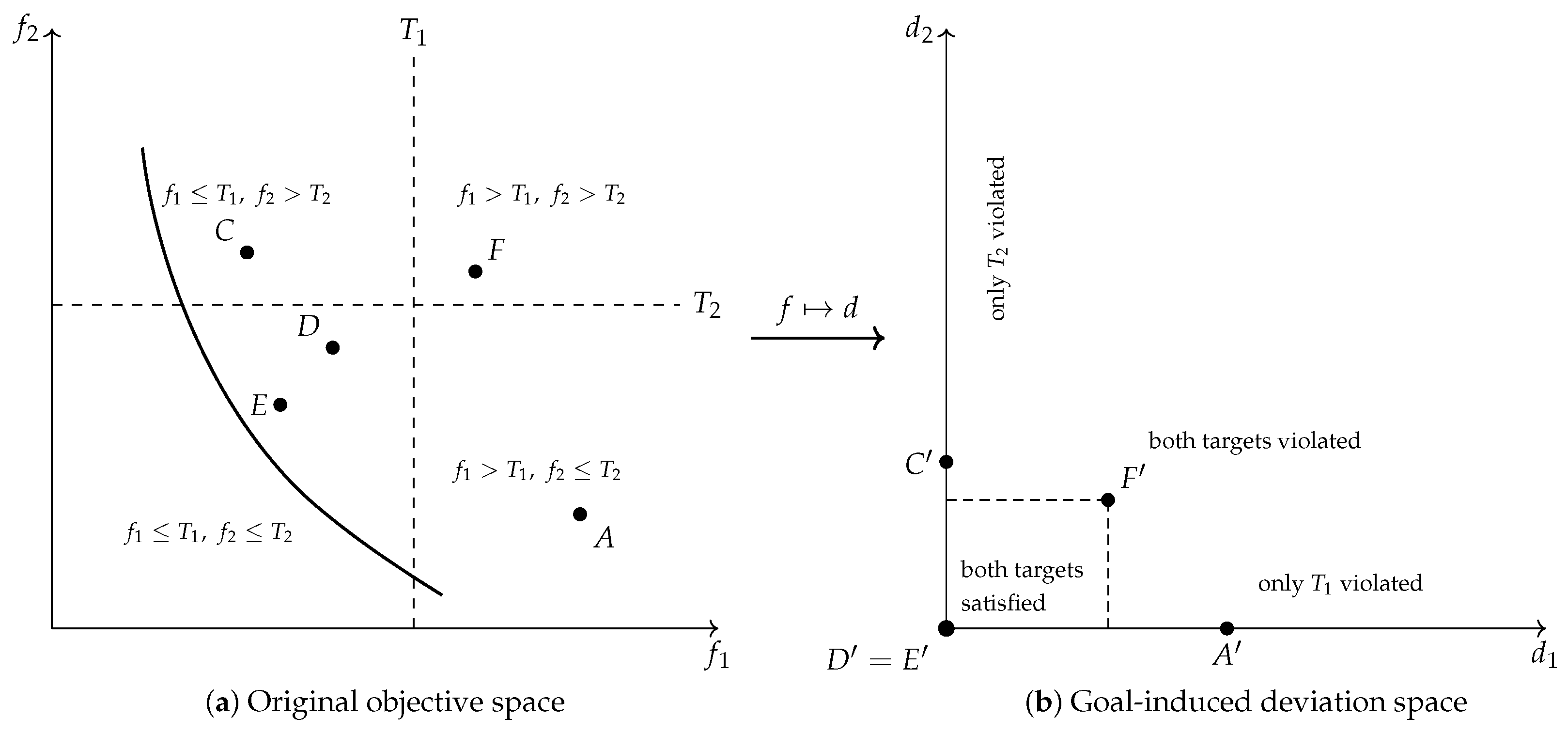
To illustrate the loss of discrimination induced by attainable targets, Figure 1 provides a geometric interpretation of the goal-induced transformation in the bi-objective case. The target levels $T_1$ and $T_2$ partition the original objective space into regions with different target violation patterns. The figure highlights that the mapping $f\mapsto d$ does not merely rescale the original objective vectors but may also project them onto the coordinate axes or collapse them to the origin whenever one or both targets is/are attained.

In panel (a), the curve represents the Pareto front of a bi-objective minimization problem. Point C satisfies the first target but violates the second one and is, therefore, mapped to the $d_2$-axis in panel (b). Point A violates only the first target and is mapped to the $d_1$-axis. Point F violates both targets and remains in the interior of the deviation space. By contrast, points D and E are distinct solutions in the original objective space that satisfy both targets and are both mapped to the origin so that $D^{\prime }=E^{\prime }=(0,0)$. Hence, panel (b) should be interpreted as the image of representative solutions under the mapping $f\mapsto d$ rather than as a complete efficient frontier in the deviation space. The coincidence of $D^{\prime }$ and $E^{\prime }$ illustrates the compression effect induced by the truncation operator. This geometric effect is precisely the one later examined in the routing case study, where solutions generated by GP and EGP are ranked through deviations but, ultimately, interpreted through their original values of truck time and makespan.

For the routing application, this geometric interpretation should be understood as conceptual rather than quantitative. In particular, in target-attainable regimes, all the target-satisfactory routing solutions are mapped to the origin in the deviation space, so an additional plot of actual routing solutions in that space would provide only limited practical discrimination. For this reason, the computational results are mainly represented and interpreted in the original objective space, where the operational meanings of truck time and makespan are preserved.

3.4.3. Consequences of Partial Target Attainment

When some targets are attained, the truncation operator may suppress improvements in objectives that are already below their aspiration levels. As a consequence, distinct solutions in the original objective space may become indistinguishable in the deviation space, and the associated weighted-deviation scalarization may lose discrimination among solutions that differ in their original objective values. This observation motivates the enhanced formulation introduced next.

3.5. Enhanced Goal Scalarization to Avoid Degeneracy

To overcome this limitation, we introduce an enhanced scalarization based on the standard goal constraints

$$f_i\left(x\right)+n_i-p_i=T_i,n_i\ge 0,p_i\ge 0,i=1,\dots ,m,$$

where $p_i$ represents underachievement (target violation), and $n_i$ represents overachievement (improvement beyond the target). Lexicographic and hierarchical refinements of this type are classical in goal programming and multicriterion optimization; see [12,16,20,25].

Lemma 1.

Under the goal constraints

$$f_i\left(x\right)+n_i-p_i=T_i,n_i,p_i\ge 0,$$

at most, one of the variables $n_i$ and $p_i$ can be positive for each objective, i. In particular,

$$n_i{p}_i=0,i=1,\dots ,m.$$

Proof. 

From the goal constraint,

$$f_i\left(x\right)+n_i-p_i=T_i,$$

we obtain

$$p_i-n_i=f_i\left(x\right)-T_i.$$

Since $n_i\ge 0$ and $p_i\ge 0$, the sign of $f_i\left(x\right)-T_i$ determines which of the two variables may be positive. If $f_i\left(x\right)>T_i$ then $p_i>0$ and, necessarily, $n_i=0$. If $f_i\left(x\right)<T_i$. Then, $n_i>0$ and, necessarily, $p_i=0$. If $f_i\left(x\right)=T_i$ then $n_i=p_i=0$. Therefore, at most, one of $n_i$ and $p_i$ can be positive, and, thus, $n_i{p}_i=0$.    □

We define the composite objective function,

$$G\left(x\right)={\displaystyle \sum _{i=1}^m}{w}_i{p}_i-\epsilon {\displaystyle \sum _{i=1}^m}{w}_i{n}_i,$$

where $w_i>0$, and $0<\epsilon$ is sufficiently low.

The first term minimizes target violations, whereas the second term favors higher overachievement when the level of the violation is the same. By Lemma 1, the second term is active only when the corresponding target is satisfied.

Proposition 6.

Let

$$G\left(x\right)={\displaystyle \sum _{i=1}^m}{w}_i{p}_i-\epsilon {\displaystyle \sum _{i=1}^m}{w}_i{n}_i,$$

with $w_i>0$, and define

$$P\left(x\right)={\displaystyle \sum _{i=1}^m}{w}_i{p}_i,N\left(x\right)={\displaystyle \sum _{i=1}^m}{w}_i{n}_i.$$

Assume that the feasible set is finite. Then, there exists $\overline{\epsilon }>0$ such that for every $0<\epsilon <\overline{\epsilon }$, minimizing $G\left(x\right)$ is equivalent to the following lexicographic procedure:

$$\min P\left(x\right),$$

followed by

$$\max N\left(x\right)$$

over the set of minimizers of the first objective.

Proof. 

Since the feasible set is finite, the set of values taken by $P\left(x\right)$ is also finite. Let

$$P^{*}=\min \{P\left(x\right):x\mathrm{feasible}\}$$

and define the set of minimizers of the first term as

$${\mathcal{S}}^{*}=\{x:x\mathrm{feasible}\mathrm{and}P\left(x\right)=P^{*}\}.$$

If all the feasible solutions belong to ${\mathcal{S}}^{*}$ then $P\left(x\right)$ is constant on the feasible set, and minimizing $G\left(x\right)=P\left(x\right)-\epsilon N\left(x\right)$ is clearly equivalent to maximizing $N\left(x\right)$. The result then follows immediately.

Assume, now, that there exists at least one feasible solution outside ${\mathcal{S}}^{*}$. Since the feasible set is finite, the positive quantity

$${\Delta }_P=\min \{P\left(x\right)-P^{*}:x\mathrm{feasible},x\notin {\mathcal{S}}^{*}\}$$

is well defined. Also, since the feasible set is finite, $N\left(x\right)$ is bounded, so there exists

$$N_{\max }=\max \{N\left(x\right):x\mathrm{feasible}\},N_{\min }=\min \{N\left(x\right):x\mathrm{feasible}\}.$$

Hence,

$${\Delta }_N:=N_{\max }-N_{\min }<\infty .$$

Choose $0<\overline{\epsilon }<{\Delta }_P/{\Delta }_N$ when ${\Delta }_N>0$; if ${\Delta }_N=0$, any $\overline{\epsilon }>0$ suffices. Let $0<\epsilon <\overline{\epsilon }$.

Consider any $x\notin {\mathcal{S}}^{*}$ and any $y\in {\mathcal{S}}^{*}$. Then,

$$P\left(x\right)\ge P^{*}+{\Delta }_P,P\left(y\right)=P^{*},$$

and, therefore,

$$G\left(x\right)-G\left(y\right)=\left(P\left(x\right)-P\left(y\right)\right)-\epsilon \left(N\left(x\right)-N\left(y\right)\right)\ge {\Delta }_P-\epsilon {\Delta }_N>0.$$

So, no feasible solution with $P\left(x\right)>P^{*}$ can minimize $G\left(x\right)$. Hence, every minimizer of $G\left(x\right)$ must belong to ${\mathcal{S}}^{*}$.

Restricted to ${\mathcal{S}}^{*}$, the term $P\left(x\right)$ is constant, and, thus, minimizing $G\left(x\right)=P^{*}-\epsilon N\left(x\right)$ is equivalent to maximizing $N\left(x\right)$. Therefore, minimizing $G\left(x\right)$ is equivalent to first minimizing $P\left(x\right)$ and then maximizing $N\left(x\right)$ over the minimizers of the first term.    □

This result justifies the interpretation of the enhanced scalarization as a single-objective implementation of a lexicographic preference structure. In the combinatorial setting considered in this paper, where the feasible set is finite, a sufficiently low value of $\epsilon$ guarantees that the weighted-violation term retains priority, while the weighted-overachievement term acts only as a tie-breaking device among solutions with the same violation level. Hence, the enhanced formulation provides a practical scalar implementation of the lexicographic refinement classically used in hierarchical goal programming; see [12,16,20].

Remark 4.

In the combinatorial setting considered in this paper, the previous result provides the theoretical basis for using the enhanced objective as a single scalar function within the search procedure. In particular, once ε is chosen to be low enough, the minimization of $G\left(x\right)$ preserves the intended priority structure: first, reducing target violations and, then, favoring overachievement among solutions with the same violation level.

The next result establishes the consistency of the enhanced formulation with Pareto efficiency in the original objective space. The proof relies on the lexicographic equivalence established in Proposition 6.

Proposition 7.

Assume that the feasible set is finite, and consider the enhanced scalarization

$$G\left(x\right)={\displaystyle \sum _{i=1}^m}{w}_i{p}_i-\epsilon {\displaystyle \sum _{i=1}^m}{w}_i{n}_i,$$

with $w_i>0$ and $0<\epsilon <\overline{\epsilon }$, where $\overline{\epsilon }$ is as in Proposition 6 under the goal constraints

$$f_i\left(x\right)+n_i-p_i=T_i,n_i,p_i\ge 0,i=1,\dots ,m.$$

Then, every optimal solution of the enhanced problem is Pareto efficient for the original objective vector, $(f_1,\dots ,f_m)$.

Proof. 

By Proposition 6, since the feasible set is finite and $0<\epsilon <\overline{\epsilon }$, minimizing

$$G\left(x\right)=P\left(x\right)-\epsilon N\left(x\right)$$

is equivalent to the lexicographic procedure

$$\min P\left(x\right),\mathrm{followed}\mathrm{by}\max N\left(x\right)$$

over the set of minimizers of $P\left(x\right)$, where

$$P\left(x\right)={\displaystyle \sum _{i=1}^m}{w}_i{p}_i,N\left(x\right)={\displaystyle \sum _{i=1}^m}{w}_i{n}_i.$$

Assume, for contradiction, that $x^{*}$ is optimal for the enhanced problem but is not Pareto efficient for the original objective vector, $(f_1,\dots ,f_m)$. Then, there exists $y\in \mathcal{X}$ such that

$$f_i\left(y\right)\le f_i\left(x^{*}\right),i=1,\dots ,m,$$

with at least one strict inequality.

From the goal constraints,

$$f_i\left(x\right)+n_i\left(x\right)-p_i\left(x\right)=T_i,i=1,\dots ,m,$$

we have

$$p_i\left(x\right)-n_i\left(x\right)=f_i\left(x\right)-T_i.$$

Hence, if $f_i\left(y\right)\le f_i\left(x^{*}\right)$ then, necessarily,

$$p_i\left(y\right)\le p_i\left(x^{*}\right).$$

Moreover, if 

$$p_i\left(y\right)=p_i\left(x^{*}\right)$$

then the improvement in $f_i$ cannot be absorbed by a higher violation term, and,  therefore,

$$n_i\left(y\right)\ge n_i\left(x^{*}\right).$$

Since y strictly improves upon $x^{*}$ in at least one original objective, there exists at least one index, k, such that either

$$p_k\left(y\right)<p_k\left(x^{*}\right)$$

or

$$p_k\left(y\right)=p_k\left(x^{*}\right)\mathrm{and}{n}_k\left(y\right)>n_k\left(x^{*}\right).$$

Multiplying by the positive weights, $w_i>0$, and summing over all the components, it follows that

$$P\left(y\right)\le P\left(x^{*}\right).$$

Furthermore, if equality holds, that is, if 

$$P\left(y\right)=P\left(x^{*}\right),$$

then since all the weights are strictly positive, and $p_i\left(y\right)\le p_i\left(x^{*}\right)$ for every i, one must have

$$p_i\left(y\right)=p_i\left(x^{*}\right),i=1,\dots ,m.$$

Hence,

$$n_i\left(y\right)\ge n_i\left(x^{*}\right),i=1,\dots ,m,$$

and because at least one original objective is strictly improved, there exists at least one index, k, such that

$$n_k\left(y\right)>n_k\left(x^{*}\right).$$

Therefore,

$$N\left(y\right)>N\left(x^{*}\right).$$

Therefore, y is lexicographically better than $x^{*}$: Either it has a strictly lower value of P, or it has the same value of P and a strictly higher value of N. By Proposition 6, this contradicts the optimality of $x^{*}$.

Hence, every optimal solution of the enhanced problem must be Pareto efficient for the original objective vector, $(f_1,\dots ,f_m)$.    □

Remark 5.

Proposition 7 shows that under the stated assumptions, the enhanced scalarization avoids the degeneracy of the classical deviation model in target-attainable regimes by selecting solutions that are Pareto efficient in the original objective space.

Proposition 8.

Consider the enhanced scalarization

$$G\left(x\right)={\displaystyle \sum _{i=1}^m}{w}_i{p}_i-\epsilon {\displaystyle \sum _{i=1}^m}{w}_i{n}_i,$$

under the goal constraints

$$f_i\left(x\right)+n_i-p_i=T_i,i=1,\dots ,m.$$

If for every feasible solution it holds that

$$f_i\left(x\right)>T_i,i=1,\dots ,m,$$

then minimizing $G\left(x\right)$ is equivalent to minimizing the weighted sum

$${\displaystyle \sum _{i=1}^m}{w}_i{f}_i\left(x\right).$$

Proof. 

If $f_i\left(x\right)>T_i$ then from the goal constraints, we obtain

$$p_i=f_i\left(x\right)-T_i,n_i=0,i=1,\dots ,m.$$

Substituting into $G\left(x\right)$ gives

$$G\left(x\right)={\displaystyle \sum _{i=1}^m}{w}_i(f_i\left(x\right)-T_i)={\displaystyle \sum _{i=1}^m}{w}_i{f}_i\left(x\right)-{\displaystyle \sum _{i=1}^m}{w}_i{T}_i.$$

Since the second term is constant with respect to x, minimizing $G\left(x\right)$ is equivalent to minimizing

$${\displaystyle \sum _{i=1}^m}{w}_i{f}_i\left(x\right).$$

   □

The main implications of the previous results for classical GP and enhanced GP under the different target-attainment regimes are summarized in

Table 1. Behaviors of classical GP and enhanced GP under different target-attainment regimes.

Case	Classical GP	Enhanced GP
All the targets are violated	Weighted sum	Weighted sum
Some targets are attained	Possible loss of discrimination	Restores discrimination and Pareto efficiency
All the targets are attainable	Degenerate	Pareto-efficient selection among target-satisfactory solutions

.

Hence, the enhanced model preserves the weighted-sum behavior of the classical formulation in the case of the uniform target violation.

The previous results show that the proposed enhanced formulation preserves the main properties of classical goal programming while avoiding its main limitation when the targets are attainable.

When the target vector is unattainable, the deviation-based model does not create satisfactory solutions but only reinterprets the original tradeoffs in terms of target nonachievement. When some targets are attained, the classical deviation model may lose discrimination among solutions that differ in the original objective space. Finally, when all the targets are attainable, the enhanced formulation eliminates the degeneracy of the classical deviation model and selects Pareto-efficient solutions among all the target-satisfactory solutions.

These properties justify the use of the proposed formulation as a goal-oriented scalarization that remains consistent with multiobjective efficiency across the different target-attainment regimes. Although each ingredient is related to existing results in goal programming and scalarization theory, the previous analysis provides a unified characterization of the behaviors of the goal-induced and enhanced formulations according to the position of the target vector.

3.6. Illustrative Theoretical Case

To complement the previous structural results, we introduce a simple bi-objective example in which the different target regimes can be analyzed explicitly. Consider the problem

$$\min \left(f_1(x,y),f_2(x,y)\right)$$

subject to

$${\displaystyle \frac{1}{2}}\le x\le {\displaystyle \frac{3}{2}},y\in \mathbb{R},$$

where

$$f_1(x,y)=x^2+y^2,f_2(x,y)={(x-2)}^2+y^2.$$

This example is useful because the original Pareto-efficient set, the classical goal-programming scalarization, and the enhanced goal-programming formulation can all be characterized in closed form.

First, observe that any feasible point with $y\ne 0$ is dominated by $(x,0)$ since

$$f_1(x,0)=x^2<x^2+y^2=f_1(x,y),$$

and

$$f_2(x,0)={(x-2)}^2<{(x-2)}^2+y^2=f_2(x,y).$$

Hence, every Pareto-efficient solution must satisfy $y=0$. Restricting, therefore, attention to points of the form $(x,0)$, with $x\in [1/2,3/2]$, one has

$$f_1(x,0)=x^2,f_2(x,0)={(x-2)}^2.$$

Along this interval, decreasing x improves $f_1$ but worsens $f_2$, whereas increasing x has the opposite effect. Therefore, the Pareto-efficient set of the original problem is

$${\mathcal{E}}_f=\left\{(x,0):{\displaystyle \frac{1}{2}}\le x\le {\displaystyle \frac{3}{2}}\right\}.$$

This explicit efficient set makes it possible to illustrate directly the two target-attainment regimes discussed in the previous subsections.

3.6.1. Target-Unattainable Regime

Consider first the target vector,

$$(T_1,T_2)=\left({\displaystyle \frac{1}{4}},{\displaystyle \frac{1}{4}}\right).$$

Since for every feasible $(x,y)$,

$$f_1(x,y)\ge {\displaystyle \frac{1}{4}},f_2(x,y)\ge {\displaystyle \frac{1}{4}},$$

and both equalities cannot hold simultaneously, the target vector is jointly unattainable.

Under this choice of targets, the classical goal-programming objective is

$${\Phi }_{\mathrm{GP}}(x,y)=w_1{[f_1(x,y)-T_1]}_{+}+w_2{[f_2(x,y)-T_2]}_{+},w_1,w_2>0.$$

Since for every feasible $(x,y)$, one has

$$f_1(x,y)\ge T_1,f_2(x,y)\ge T_2,$$

the truncation operator is inactive in both components, and, therefore,

$${[f_i(x,y)-T_i]}_{+}=f_i(x,y)-T_i,i=1,2.$$

Hence, this scalarization is equivalent to minimizing

$$w_1{f}_1(x,y)+w_2{f}_2(x,y).$$

Substituting the expressions of $f_1$ and $f_2$, one obtains

$$w_1{f}_1(x,y)+w_2{f}_2(x,y)=w_1{x}^2+w_2{(x-2)}^2+(w_1+w_2)y^2.$$

Since $w_1+w_2>0$, the optimal value of y is

$$y^{★}=0.$$

The problem thus reduces to

$$\underset{{\displaystyle \frac{1}{2}}\le x\le {\displaystyle \frac{3}{2}}}{\min }\left[w_1{x}^2+w_2{(x-2)}^2\right].$$

Differentiating with respect to x yields

$$2w_{1}x+2w_2(x-2)=0,$$

and, therefore, the unconstrained minimizer is

$$x^{\circ }={\displaystyle \frac{2w_2}{w_1+w_2}}.$$

Taking into account the feasible interval, the selected solution is

$$x^{★}=\left\{\begin{array}{cc}{\displaystyle \frac{1}{2}},\hfill & \mathrm{if}{\displaystyle \frac{2w_2}{w_1+w_2}}<{\displaystyle \frac{1}{2}},\hfill \\ {\displaystyle \frac{2w_2}{w_1+w_2}},\hfill & \mathrm{if}{\displaystyle \frac{1}{2}}\le {\displaystyle \frac{2w_2}{w_1+w_2}}\le {\displaystyle \frac{3}{2}},\hfill \\ {\displaystyle \frac{3}{2}},\hfill & \mathrm{if}{\displaystyle \frac{2w_2}{w_1+w_2}}>{\displaystyle \frac{3}{2}}.\hfill \end{array}\right.$$

Hence, for every choice, $w_1,w_2>0$, the solution returned by classical GP belongs to ${\mathcal{E}}_f$. In other words, when the target vector is unattainable, the weights do not change the efficient set itself but only determine which Pareto-efficient point is selected on the original frontier. The same conclusion applies to the enhanced formulation since in this regime, it reduces to the same effective selection criterion.

3.6.2. Target-Attainable Regime

Consider, now, the target vector

$$(T_1,T_2)=\left({\displaystyle \frac{9}{4}},{\displaystyle \frac{9}{4}}\right).$$

In this case, every point, $(x,0)$, with $x\in [1/2,3/2]$, satisfies both targets because 

$$x^2\le {\displaystyle \frac{9}{4}},{(x-2)}^2\le {\displaystyle \frac{9}{4}}.$$

Moreover, there also exist dominated feasible solutions satisfying both targets. For example, if $x=1$ then

$$f_1(1,y)=f_2(1,y)=1+y^2,$$

so every point, $(1,y)$, such that

$$0<\left|y\right|\le {\displaystyle \frac{\sqrt{5}}{2}},$$

satisfies

$$f_1(1,y)\le {\displaystyle \frac{9}{4}},f_2(1,y)\le {\displaystyle \frac{9}{4}},$$

while being dominated by $(1,0)$.

Therefore, under classical GP, all the target-satisfactory feasible solutions have zero positive deviations and are optimal for ${\Phi }_{\mathrm{GP}}$. This illustrates the loss of discrimination of the classical formulation in the target-attainable regime: Satisfactory solutions may be selected even if they are dominated in the original objective space.

To avoid this degeneracy, consider the enhanced goal-programming objective,

$$G(x,y)=w_1{p}_1+w_2{p}_2-\epsilon (w_1{n}_1+w_2{n}_2),w_1,w_2>0,\epsilon >0,$$

under the goal constraints

$$f_i(x,y)+n_i-p_i=T_i,n_i\ge 0,p_i\ge 0,i=1,2.$$

Inside the target-satisfactory region, one has $p_1=p_2=0$, and, thus, minimizing $G(x,y)$ is equivalent to maximizing

$$w_1{n}_1+w_2{n}_2.$$

Since

$$n_1=T_1-f_1(x,y)={\displaystyle \frac{9}{4}}-f_1(x,y),n_2=T_2-f_2(x,y)={\displaystyle \frac{9}{4}}-f_2(x,y),$$

this is equivalent to minimizing

$$w_1{f}_1(x,y)+w_2{f}_2(x,y).$$

Consequently, the enhanced formulation again yields $y^{★}=0$ and selects

$$x^{★}=\left\{\begin{array}{cc}{\displaystyle \frac{1}{2}},\hfill & \mathrm{if}{\displaystyle \frac{2w_2}{w_1+w_2}}<{\displaystyle \frac{1}{2}},\hfill \\ {\displaystyle \frac{2w_2}{w_1+w_2}},\hfill & \mathrm{if}{\displaystyle \frac{1}{2}}\le {\displaystyle \frac{2w_2}{w_1+w_2}}\le {\displaystyle \frac{3}{2}},\hfill \\ {\displaystyle \frac{3}{2}},\hfill & \mathrm{if}{\displaystyle \frac{2w_2}{w_1+w_2}}>{\displaystyle \frac{3}{2}}.\hfill \end{array}\right.$$

Hence, unlike classical GP, the enhanced formulation restores discrimination and returns a Pareto-efficient solution of the original problem.

3.6.3. The Practical Role of $\epsilon$

Let

$$P(x,y)=w_1{p}_1+w_2{p}_2,N(x,y)=w_1{n}_1+w_2{n}_2.$$

Since $0\le n_i\le T_i$, one has

$$0\le N(x,y)\le w_1{T}_1+w_2{T}_2.$$

Therefore, if ${\Delta }_P>0$ denotes the minimum positive variation in $P(x,y)$. Consistent with the numerical precision used in the reporting of the objective values, a sufficient condition is

$$0<\epsilon <{\displaystyle \frac{{\Delta }_P}{w_1{T}_1+w_2{T}_2}}.$$

Under this condition, the improvement induced by the overachievement term can never compensate for a relevant deterioration in the weighted-violation term. In this way, the enhanced formulation preserves the intended hierarchy directly within the scalar objective actually used by the search procedure.

For the attainable-target configuration considered above, this bound becomes

$$0<\epsilon <{\displaystyle \frac{{\Delta }_P}{\frac{9}{4}(w_1+w_2)}}.$$

This example confirms in a completely explicit setting the behavior described by the general theory. When the target vector is unattainable, classical GP and enhanced GP both reduce to the selection of a Pareto-efficient point which location depends on the relative values of $w_1$ and $w_2$. When the target vector is attainable, classical GP may admit dominated target-satisfactory solutions, whereas the enhanced formulation restores discrimination and remains consistent with Pareto efficiency. This theoretical case also anticipates the two computational regimes analyzed later in the routing problem: a target-unattainable regime, in which classical GP and enhanced GP coincide, and a target-attainable regime, in which the enhanced formulation avoids the loss of discrimination of classical GP.

In practical implementations, a sufficient condition is to choose

$$0<\epsilon <{\displaystyle \frac{{\Delta }_P}{w_1{T}_1+w_2{T}_2}},$$

where ${\Delta }_P>0$ denotes the minimum relevant positive variation in the primary term, $P(x,y)$. Under this condition, the improvement induced by the overachievement term cannot compensate for a relevant deterioration in the weighted-violation term. Thus, the intended priority structure is preserved in the scalar objective used by the search procedure.

3.7. Bi-Criterion Truck–Multiple-Drone Routing Problem and Case-Study Methodology

The application setting considered in this paper is a bi-criterion version of the truck–multiple-drone routing problem previously studied in [7]. A single truck cooperates with a fleet of drones to serve a set of customer nodes. Both the truck and the drones may serve customers; drones may perform multi-visit missions between synchronization points, and rendezvous locations need not coincide with launch nodes. The truck is assumed to have unlimited operational autonomy, whereas each drone is subject to a limited flight endurance. Whenever a drone meets the truck at a synchronization node, its autonomy is restored. As in the reference framework, waiting may occur at synchronization nodes.

3.7.1. Problem Setting

The experiments are conducted on instances extracted from the uniform benchmark set introduced by Agatz et al. and adopted in the baseline bi-criterion study. In the present paper, the illustrative analysis is based on representative instances with 20 and 50 nodes, while the broader benchmark battery includes instances with 20 nodes and two drones and instances with 50 nodes and three drones. These settings are sufficiently rich to exhibit nontrivial tradeoffs while still allowing a clear graphical interpretation of the estimated efficient sets and of the corresponding target-induced transformations. As in the baseline setting, the routing structure is defined on an open route from a given origin node to a distinct destination node rather than on a closed depot-to-depot tour.

Regarding travel parameters, the same assumptions as those in the reference bi-criterion framework are maintained. In particular, the drone speed is taken to be twice the truck speed. Under this assumption, the truck usage can be measured equivalently through the truck travel time or, up to a constant proportionality factor through the truck distance. Likewise, the drone endurance parameter, Q, is fixed according to the same calibration adopted in the underlying routing model; detailed instance generation and parameter-setting issues can be found in [7].

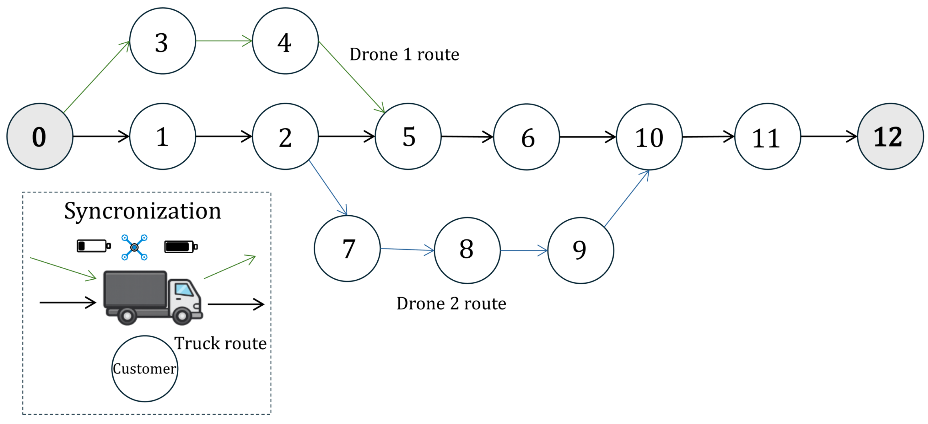
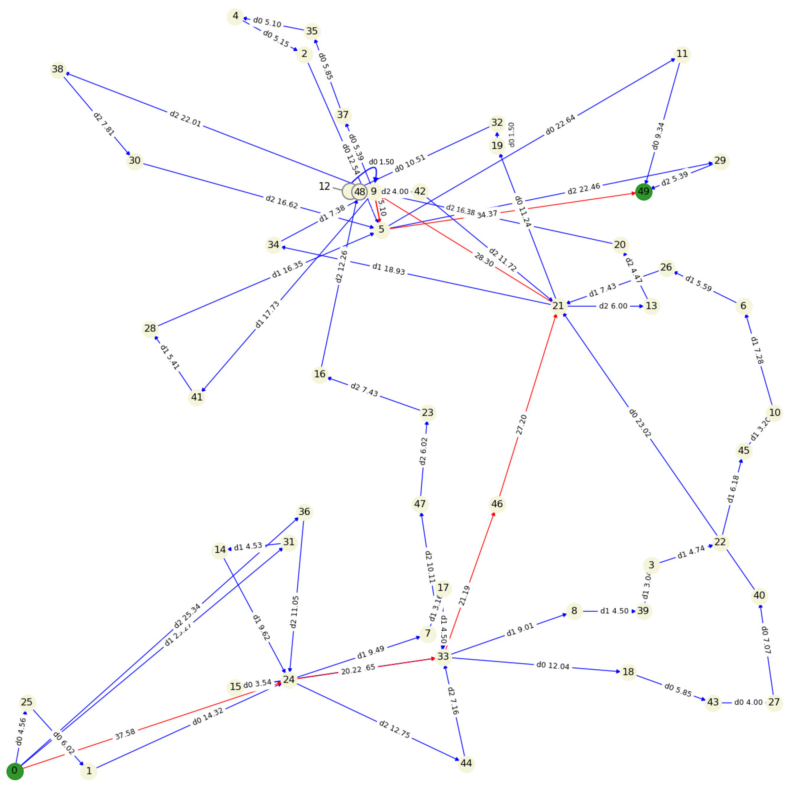
To illustrate the collaborative structure underlying the routing problem, Figure 2 shows a stylized feasible solution involving one truck and two drones. The figure highlights the coexistence of truck movements, drone missions, and synchronization points at which aerial resources rejoin the truck and recover autonomy.

Let $x\in \mathcal{X}$ denote a feasible routing and synchronization plan. For each feasible solution, two original objective functions are considered. The first one, $f_1\left(x\right)$, measures the truck usage, expressed here as the truck travel time, (Truck Time). Under the adopted speed assumptions, this criterion is also proportional to the truck distance. The second one, $f_2\left(x\right)$, measures the total service completion time, i.e., the makespan. Therefore, the original bi-criterion routing problem can be written as

$$\min \left(f_1\left(x\right),f_2\left(x\right)\right),x\in \mathcal{X},$$

where the first component represents the truck usage, and the second one represents the overall mission duration. This ordering is also the one used later in the Pareto-front plots, where the horizontal axis corresponds to the truck time, and the vertical axis corresponds to the makespan.

3.7.2. Solution Procedure

The computational study relies on the agent-based metaheuristic proposed by León-Blanco et al. [4], originally developed for the single-objective truck–multidrone team logistics problem. This search framework was selected because all the optimization tasks required in the present paper are scalar optimization problems. In particular, it is used (i) to estimate a reference Pareto frontier in the original objective space through repeated weighted-sum runs, (ii) to solve the classical goal-programming (GP) scalarization, and (iii) to solve the enhanced goal-programming (EGP) scalarization. Using a common search engine in these three settings makes it possible to change only the driving objective function while preserving the same underlying optimization mechanism.

At a high level, the method is a cooperative multi-agent search procedure in which agents represent customer locations. Solutions are encoded on a two-dimensional grid that simultaneously captures the visit order and vehicle assignment. A manager agent constructs an initial feasible solution, maintains an asynchronous memory of solutions, coordinates the search, and activates diversification steps when no improving move is found. The local search mechanism is based on neighborhood moves that modify the position of a location in the grid, reassign a location to a different vehicle/meeting pattern, or insert it into a nearby route segment. In particular, the search uses the move operators yMove(), 2opt(), and node2arc() together with the diversification procedure rand_sol(), as defined in [4].

To improve reproducibility, the main operational settings adopted in the present paper are summarized next. Each scalar optimization run starts from a feasible constructive initialization generated by the manager agent. The search is then iteratively improved by the neighborhood operators indicated above. A time budget of 600 s is assigned to each scalar run, and 10 independent runs are performed for each scalar objective configuration. Unless otherwise stated, the best solution found over those runs is retained for the subsequent analysis.

Since the present work is focused on the target-oriented decision framework rather than on a new parameter-tuning study, the search parameters were fixed in advance and kept identical across all the scalar optimization tasks associated with the same instance size. The notation and the role of these parameters follow León-Blanco et al. [4]. In particular, pfactor is the penalty multiplier applied when temporarily infeasible solutions violate the drone endurance constraint. The parameter max r is used to compute the maximum swapping radius in the horizontal movement operator, 2opt(), whereas R controls the number of agents extracted and reinserted in the random reconstruction procedure, rand_sol(). Finally, max its denotes the maximum number of iterations allowed inside rand_sol().

Because the computational experiments reported below involve two benchmark sizes, the values of the size-dependent parameters are reported separately for $n=20$ and $n=50$, as summarized in

Table 2. Agent-based search parameters adopted in the computational study.

Parameter	$\mathit{n}=20$	$\mathit{n}=50$	Brief Role in the Search
pfactor	1.0	1.0	Penalty multiplier for solutions violating drone endurance
max r	10	20	Parameter used to compute the maximum horizontal swapping radius in 2opt()
R	10	20	Parameter used to compute the number of extracted agents in rand_sol()
max its	20	30	Maximum number of iterations in the rand_sol() procedure
Runtime budget	600 s	600 s	Time limit assigned to each scalar optimization run
Independent runs	10	10	Number of repeated runs per scalar objective configuration

. The specific instances and target scenarios are described in Section 3.7.3 and Section 3.7.4.

The same parameter setting was used for the reference frontier estimation, the GP scalarizations, and the EGP scalarizations so that differences in the reported solutions are attributable to the scalar objective function rather than to changes in the underlying search engine. The estimation of the reference Pareto frontier and the target-oriented evaluation protocol are described in Section 3.7.3 and Section 3.7.4, respectively.

3.7.3. Reference Pareto Frontier Estimation

In contrast to the purely theoretical developments of the previous subsections, the efficient frontier of the routing problem is not known in a closed form. Moreover, because of the combinatorial complexity of the truck–multiple-drone problem, the true Pareto front is generally unavailable, even for moderately sized instances. For this reason, the original non-dominated set is estimated heuristically in the original objective space.

More specifically, the reference frontier used in the computational study is obtained by solving a family of scalarized bi-criterion routing problems of the form

$$\alpha f_1\left(x\right)+(1-\alpha )f_2\left(x\right),\alpha \in [0,1]$$

for different values of $\alpha$ and then retaining the non-dominated solutions obtained. For each value of $\alpha$, 10 independent runs of the agent-based search procedure are performed, and the resulting objective vectors are retained. The non-dominated subset extracted from the resulting cloud of solutions is then used to construct the estimated reference Pareto frontier. This procedure is computationally demanding because it requires multiple independent heuristic runs in order to obtain a sufficiently rich approximation of the efficient frontier. Therefore, the frontier used in the computational study should be interpreted as a heuristic reference frontier. Accordingly, the conclusions drawn in the routing case study are made with respect to this estimated frontier, whereas the theoretical distinction between GP and EGP is additionally supported by the illustrative analytical example, in which the Pareto frontier is known exactly.

3.7.4. Target-Oriented Evaluation Protocol

Once a reference frontier has been estimated in the original objective space, it is used as the benchmark structure for the target-oriented analysis developed in this paper. More specifically, for each selected instance, the scalarized problem

$$\alpha f_1\left(x\right)+(1-\alpha )f_2\left(x\right)$$

is solved for

$$\alpha \in \{0,0.1,0.2,\dots ,0.9,1\}$$

by performing 10 independent runs for each value of $\alpha$. This yields a set of $11\times 10=110$ solutions in the original objective space, from which the non-dominated subset is extracted and taken as the estimated reference Pareto frontier.

Let

$${\widehat{z}}^I=\left(\min \left\{f_1\left(x\right)\right\},\min \left\{f_2\left(x\right)\right\}\right)$$

denote the estimated ideal point computed from these 110 solutions. Based on this point, two target regimes are considered:

$$T^U={\widehat{z}}^I,T^A=1.30{\widehat{z}}^I.$$

The first one represents the unattainable-target regime, whereas the second one is used as a relaxed target vector intended to represent an attainable regime.

These target vectors are introduced here as illustrative case-dependent choices for the computational study. In accordance with standard goal programming, the weights and targets are not parameters generated by the method itself but are exogenous preference inputs provided by the decision maker. Therefore, the specific values adopted in the experiments should not be interpreted as a universal rule for parameter selection, but as operational choices aimed at instantiating the two target regimes studied theoretically in this paper.

Once the target vectors have been defined, each solution of the estimated frontier can be represented with respect to a target vector, $T=(T_1,T_2)$, through the normalized deviation mapping,

$$d\left(x\right)=\left({\displaystyle \frac{{[f_1\left(x\right)-T_1]}_{+}}{T_1}},{\displaystyle \frac{{[f_2\left(x\right)-T_2]}_{+}}{T_2}}\right),$$

where $T_1$ is the aspiration level associated with the truck time, and $T_2$ is the aspiration level associated with the makespan. This transformation allows the original tradeoff structure to be reinterpreted in terms of target violations and makes it possible to study, in a routing context, the phenomena established in the theoretical part of the paper, including dominance preservation, the loss of discrimination, and the target-dependent compression of the efficient set.

The optimization process and the graphical analysis are, therefore, carried out in two complementary spaces. On the one hand, GP and EGP evaluate candidate routing plans through deviation-based scalarizations defined with respect to the target vector and the preference weights. On the other hand, every solution returned by these models remains a feasible solution of the original routing problem and can, therefore, be represented by its original objective vector, $(f_1\left(x\right),f_2\left(x\right))$. For this reason, the final computational analysis is reported in the original objective space, where the practical meaning of the solution can be assessed and where it can be checked whether the target-driven solution lies on the estimated Pareto frontier or is dominated by other feasible tradeoff solutions.

This choice is especially important in target-attainable regimes. In such cases, the deviation mapping may collapse several distinct routing solutions to the same point, typically the origin, when all the targets are satisfied, so a graphical representation in the deviation space may become weakly informative from a practical viewpoint. By contrast, the original objective space retains the operational differences among routing plans and, therefore, provides a more meaningful basis for the computational comparison between GP and EGP.

For each target–weight configuration, the routing problem is solved again from a goal-programming perspective. To this end, the same agent-based search framework is employed again but by replacing the original driving objective function by a deviation-based scalarization. Two goal-based variants are considered in the computational study: the classical GP formulation and the enhanced GP scalarization introduced in the previous subsections. Thus, GP and EGP do not generate the whole Pareto frontier in the original objective space; instead, they produce target-oriented routing solutions, which are subsequently represented in the original objective space and compared with the estimated reference frontier. The purpose of this comparison is not to benchmark alternative multiobjective metaheuristics but to isolate the effect of the target-based decision model itself. For this reason, classical GP and the proposed EGP are evaluated under the same search framework so that the observed differences can be attributed to the scalarization scheme rather than to changes in the underlying optimization procedure.

In all the EGP computational runs, the enhancement parameter was fixed at $\epsilon ={10}^{-4}$. This value was chosen to be sufficiently low relative to the scale of the weighted-violation term so that the primary objective of reducing target violations keeps priority over the secondary overachievement term. This choice is consistent with the sufficient condition discussed in Section 3.6.3, taking $\Delta P=0.1$ as the minimum relevant positive variation in the primary term according to the numerical precision adopted in the reporting of objective values.

It should be noted that the previous distinction is theoretical as well as computational. At the model level, classical GP may return dominated solutions when the aspiration levels are attainable, whereas Proposition 7 shows that every exact optimal solution of the enhanced formulation is Pareto efficient in the original objective space, under the stated assumptions. At the computational level, however, the routing problem is solved through a metaheuristic procedure, so no guarantee of global optimality can be claimed. Accordingly, the numerical study evaluates whether the obtained solutions are aligned with the estimated reference Pareto frontier rather than certifying efficiency with respect to the true unknown frontier.

It should also be noted that the estimation of the reference Pareto frontier is computationally more demanding than a direct target-oriented optimization run. In the illustrative experiments, the frontier is approximated from $11\times 10=110$ scalarized runs, whereas each GP or EGP configuration is solved through 10 independent runs. Thus, when the decision maker already has prescribed targets and weights, EGP offers a direct optimization mechanism, while the reference frontier is mainly useful as a benchmark and as a tool for interpreting the resulting solution in the original objective space.

Overall, this computational design is intended primarily as an illustrative application of the theoretical framework. In particular, it is used to show, on representative instances of different sizes, how the reference frontier is estimated, how the target vectors are constructed from the estimated ideal point, and how GP and EGP behave under unattainable- and attainable-target regimes.

4. Results and Discussion

This section is organized in two stages. First, two illustrative experiments are reported for representative benchmark instances with 20 and 50 nodes, namely, uniform-61-n20 and uniform-71-n50. For each of these instances, the analysis is structured around three elements: (i) the estimation of a reference Pareto frontier from repeated weighted-sum runs, (ii) the construction of unattainable- and attainable-target points from the estimated ideal point, and (iii) the comparison of the solutions obtained with GP and EGP under both target regimes.

Second, a broader computational study on a larger benchmark battery is introduced in order to compare both methods statistically. This second stage considers the minimum and average performance values and serves to assess the general behaviors of GP and EGP beyond the two illustrative instances.

Throughout this section, the original objective ordering is preserved: $f_1\left(x\right)$ denotes the truck time, and $f_2\left(x\right)$ denotes the makespan. Accordingly, in all the Pareto-front plots, the horizontal axis corresponds to the truck time, and the vertical axis corresponds to the makespan.

4.1. Illustrative Experiments on Selected Instances

Two representative instances from the uniform benchmark set are considered in order to illustrate the proposed target-oriented analysis: one instance with 20 nodes, and one instance with 50 nodes, namely, uniform-61-n20 and uniform-71-n50. In both cases, the same experimental logic is followed. First, a cloud of 110 solutions is generated by repeated weighted-sum runs with $\alpha \in \{0,0.1,\dots ,1\}$ and 10 independent replications for each value. Second, the corresponding estimated reference Pareto frontier is extracted. Third, the estimated ideal point is used to define two target regimes, namely, an unattainable one and an attainable one. Finally, the solutions obtained with GP and EGP are represented in the original objective space and compared with the estimated frontier.

The aim of these experiments is not to provide a complete empirical validation but to visualize the behaviors of the proposed framework in two representative settings of different sizes.

4.1.1. Instance uniform-61-n20

The first illustrative experiment is conducted on instance uniform-61-n20, extracted from the uniform benchmark set introduced by Agatz et al. [26] and adopted in the baseline bi-criterion routing study [7]. In this experiment, the 20-node instance is solved with a fleet composed of one truck and two drones. The reference set is obtained from 110 scalar optimization runs, corresponding to 11 values of $\alpha$ and 10 independent replications for each value, from which the estimated reference Pareto frontier is extracted.

The estimated ideal point is

$${\widehat{z}}_{20}^I=(108.19,139.93),$$

and, therefore, the two target vectors considered in this experiment are

$$T_{20}^U=(108.19,139.93),T_{20}^A=1.30{\widehat{z}}_{20}^I=(140.64,181.91).$$

Thus, $T_{20}^U$ represents the unattainable regime, whereas $T_{20}^A$ is used as a relaxed target vector intended to represent an attainable regime.

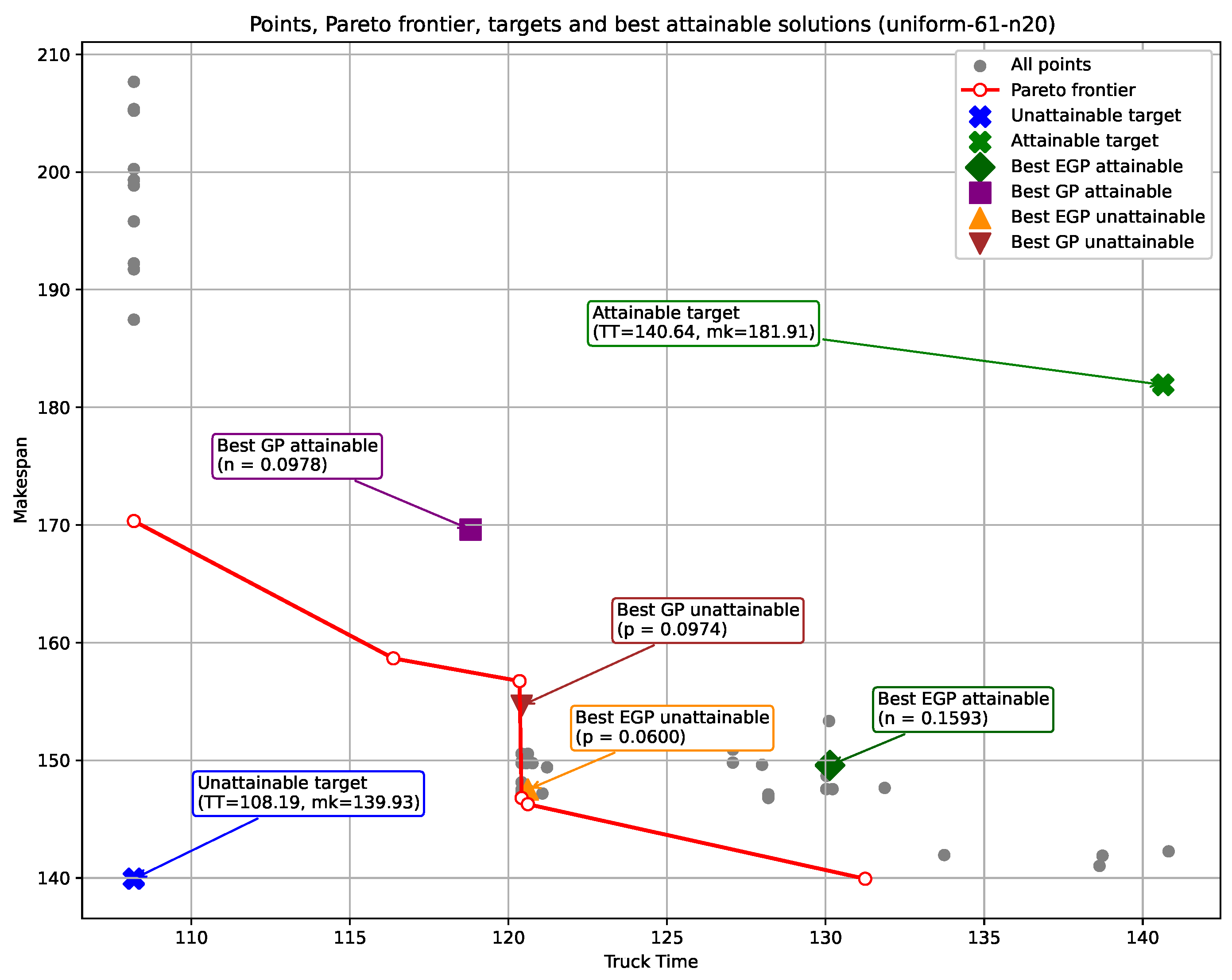
Figure 3 displays the 110-solution cloud, the estimated reference Pareto frontier, and the two target points used for the 20-node experiment. In this plot, $T_{20}^U$ corresponds to the estimated ideal point and is not jointly attained by the solutions in the reference set, whereas $T_{20}^A$ defines the relaxed target region used to illustrate the attainable-target regime.

The figure also reports the best solutions obtained with GP and EGP under both target regimes, where each reported solution corresponds to the best result found over 10 independent runs of the corresponding optimization setting. In the unattainable case, the best GP solution is $(122.00,160.00)$, whereas the best EGP solution is $(120.61,147.51)$. In the attainable case, the best GP solution is $(118.80,169.62)$, whereas the best EGP solution is $(130.14,149.57)$.

The attainable regime is especially informative. The GP solution satisfies the target levels, but classical GP does not include any explicit mechanism to continue searching for the best target-satisfactory solution once the positive deviations vanish. By contrast, EGP preserves discrimination within the target-satisfactory region through the secondary term, $N\left(x\right)={\sum }_i{w}_i{n}_i$, which favors higher-weighted overachievement beyond the targets. This effect is especially relevant once the target region has been reached. In that situation, the improvement values displayed in the figure are reported in per-unit terms and measure the weighted margin of the improvement beyond the prescribed targets. For comparability, the same indicator is computed for both methods. However, its role is different in each case: In GP, it is evaluated only a posteriori since it does not intervene in the objective function; in EGP, by contrast, it is explicitly favored by the secondary term of the scalarization. Hence, in this instance, GP reaches the target region, whereas EGP continues pushing the search toward a solution with a higher-weighted margin beyond the target and a position closer to the estimated efficient tradeoff structure.

To complement the representation in the objective space, a routing-level visualization is provided for the attainable-target regime. This is the regime in which the theoretical distinction between GP and EGP is the most relevant: Once the target region has been reached, classical GP may lose discrimination among target-satisfactory solutions, whereas EGP continues to favor solutions with a higher-weighted margin beyond the prescribed targets.

Since the routing problem is solved heuristically, these results should be interpreted with respect to the estimated frontier rather than as a certificate of the exact Pareto optimality. Nevertheless, the figure provides a compact illustration of how the target construction and the two scalarizations interact in the 20-node case.

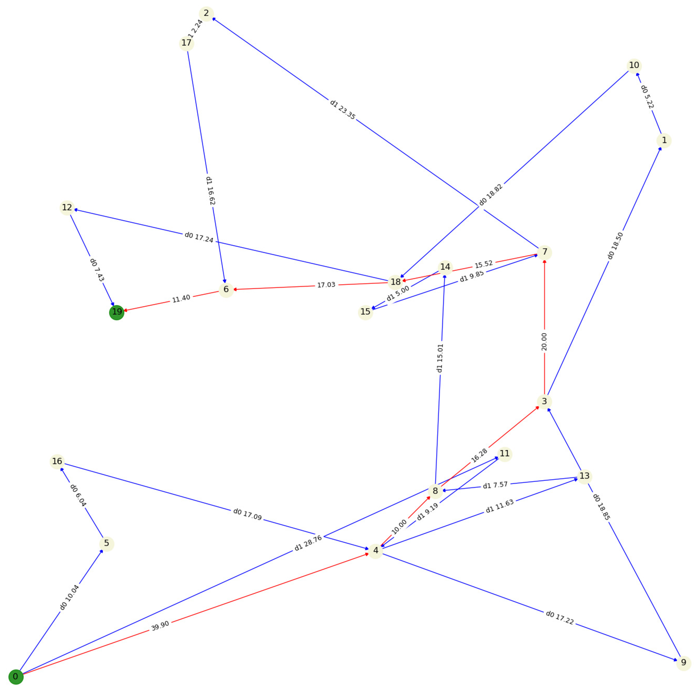
The routing plot in Figure 4 provides a complementary operational interpretation of the EGP solution displayed in Figure 3. The truck route is represented by the red line, whereas drone sorties are shown in blue. Arc labels report the corresponding travel times and, for drone flights, identify the drone assigned to each sortie. The purpose of this visualization is not to claim that EGP produces a radically different routing topology from GP but rather to illustrate the operational structure of the solution selected by the enhanced scalarization in the attainable-target regime.

This observation is consistent with the role of the enhanced scalarization. Once the target levels are satisfied, classical GP may stop discriminating among target-satisfactory alternatives. By contrast, EGP continues to exploit the secondary improvement term, thereby favoring a solution with a higher-weighted margin beyond the targets. In this instance, this additional discrimination is mainly reflected in the objective-space performance rather than in a visibly different routing topology.

4.1.2. Instance uniform-71-n50

The second illustrative experiment is conducted on instance uniform-71-n50, extracted from the uniform benchmark set introduced by Agatz et al. [26] and adopted in the baseline bi-criterion routing study [7]. In this experiment, the 50-node instance is solved with a fleet composed of one truck and three drones. The reference set is obtained from 110 scalar optimization runs, corresponding to 11 values of $\alpha$ and 10 independent replications for each value, from which the estimated reference Pareto frontier is extracted.

The estimated ideal point is

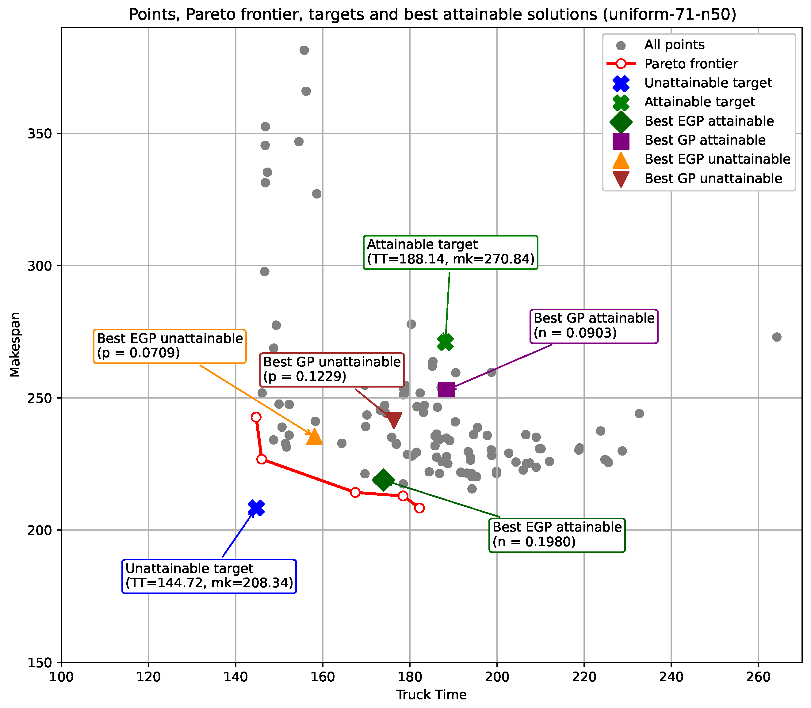
$${\widehat{z}}_{50}^I=(144.72,208.34),$$

and, therefore, the two target vectors considered in this experiment are

$$T_{50}^U=(144.72,208.34),T_{50}^A=1.30{\widehat{z}}_{50}^I=(188.14,270.84).$$

Thus, $T_{50}^U$ represents the unattainable regime, whereas $T_{50}^A$ is used as a relaxed target vector intended to represent an attainable regime.

Figure 5 shows the corresponding objective-space representation for the 50-node experiment. The same target-construction rule is applied, but the resulting comparison is more demanding from a computational viewpoint because the instance involves a larger customer set and three drones. The figure is therefore used to assess whether the behavior observed in the 20-node case is also visible in a larger routing setting.

The figure also reports the best solutions obtained with GP and EGP under both target regimes, where each reported solution corresponds to the best result found over 10 independent runs of the corresponding optimization setting. In the unattainable case, the best GP solution is approximately $(149.00,212.00)$, whereas the best EGP solution is approximately $(158.14,235.32)$. In the attainable case, the best GP solution is $(188.36,252.88)$, whereas the best EGP solution is $(173.96,218.89)$.

As in the 20-node case, the attainable regime is the most informative, although the numerical values should be interpreted with some care. The attainable-target vector defines a relaxed target region, but the best GP solution reported in this experiment lies marginally above the truck time target, $(188.36>188.14)$, while satisfying the makespan target. This is consistent with the heuristic nature of the search and with the fact that the reported point is the best solution found over 10 independent runs for the corresponding scalarization.

By contrast, the best EGP solution, $(173.96,218.89)$, satisfies both target levels and preserves discrimination within the target-satisfactory region through the secondary term, $N\left(x\right)={\sum }_i{w}_i{n}_i$, which favors higher-weighted overachievement beyond the targets. The improvement values displayed in the figure are reported in per-unit terms and measure the componentwise weighted degree of overachievement with respect to the prescribed targets. For comparability, the same indicator is computed for both methods. However, its role is different in each case: In GP, it is evaluated only a posteriori since it does not intervene in the objective function; in EGP, by contrast, it is explicitly favored by the secondary term of the scalarization.

This behavior is clearly reflected in the attainable case. The weighted improvement associated with EGP is $0.1980$, whereas the corresponding value for GP is $0.0903$. More importantly, the contrast is also visible in the original objective space: Compared with GP, the EGP solution achieves both a shorter truck time and a shorter makespan. In this instance, therefore, the advantage of EGP is not only reflected in a higher-weighted overachievement indicator but also in a solution that dominates the GP solution in the two reported objectives.

Since the routing problem is solved heuristically, these results should be interpreted with respect to the estimated frontier rather than as a certificate of the exact Pareto optimality. Nevertheless, the figure provides a compact illustration of how the target construction and the two scalarizations interact in the 50-node case.

The routing plot in Figure 6 provides a complementary operational interpretation of the EGP solution displayed in Figure 5. As in the 20-node case, the route is included only as an illustrative operational view of the solution selected by the enhanced scalarization in the attainable-target regime rather than as evidence of a radically different routing topology.

The truck route is represented by the red line, whereas drone sorties are shown in blue. Arc labels report the corresponding travel times and, for drone flights, identify the drone assigned to each sortie. In this instance, the main distinction between GP and EGP should, therefore, be interpreted primarily through their location in the $(TT,mk)$ plane and through the weighted-overachievement indicator rather than through a qualitative comparison of route shapes.

4.2. Benchmark Battery and Statistical Comparison

Beyond the two illustrative experiments discussed above, a broader benchmark battery is considered in order to compare GP and EGP over a larger collection of instances. This second stage includes instances with 20 nodes and two drones and instances with 50 nodes and three drones. For each instance, the target vectors are constructed from the estimated ideal point obtained from repeated scalarized runs, following the protocol described in Section 3.7.4.

The broader computational comparison is restricted to the attainable-target regime. The reason is that this is the setting in which the distinction between classical GP and the enhanced formulation is the most meaningful. Under unattainable targets, both models are essentially driven by the minimization of positive deviations, so the additional discrimination mechanism of EGP does not play the same role as in the target-satisfactory region. By contrast, once the targets become attainable, classical GP may lose discrimination among target-satisfactory solutions, whereas EGP is specifically designed to preserve it through the secondary term associated with weighted overachievement. For this reason, the battery study focuses on the attainable regime, where the practical differences between both scalarizations can be assessed more clearly. Although the attainable targets are generated in all the instances through the same rule, $T^A=1.30{\widehat{z}}^I$, this does not imply the same effective level of restrictiveness across the benchmark battery. The practical difficulty of the target depends not only on the multiplicative factor but also on the shape and dispersion of the estimated Pareto frontier and on the relative position of the feasible tradeoff region with respect to the estimated ideal point.

This difference is already visible in the illustrative experiments, where the 30% relaxation leads to a clearly less restrictive target in the 20-customer setting than in the 50-customer setting. Therefore, the rule $T^A=1.30{\widehat{z}}^I$ should be interpreted as a uniform target construction criterion, not as a mechanism ensuring equal target severity across instances.

For each instance and method, 10 independent runs are performed. Let n denote the signed normalized target margin. By construction, n is expressed in per-unit terms with respect to the target values. Positive values indicate that the target is attained and improved upon, zero indicates exact attainment, and negative values indicate that the target is not reached. For each instance and method, we report $n_{\mathrm{best}}$, the best signed normalized target margin over 10 runs, $n_{\mathrm{avg}}$, the corresponding average signed margin, and the target-attainment rate, defined as the number of runs, out of 10, that reach the target region. To compare both methods directly, we also define

$$D_{\mathrm{best}}=n_{\mathrm{best}}^{EGP}-n_{\mathrm{best}}^{GP},D_{\mathrm{avg}}=n_{\mathrm{avg}}^{EGP}-n_{\mathrm{avg}}^{GP}$$

so that positive values favor EGP.

Table 3. Global comparison between GP and EGP in the attainable-target regime.

Id	GP			EGP			Difference
	${\mathit{n}}_{\mathbf{best}}$	${\mathit{n}}_{\mathbf{avg}}$	Target Att. Rate	${\mathit{n}}_{\mathbf{best}}$	${\mathit{n}}_{\mathbf{avg}}$	Target Att. Rate	${\mathit{D}}_{\mathbf{best}}$	${\mathit{D}}_{\mathbf{avg}}$
61	0.0978	0.0358	9/10	0.1593	0.1390	10/10	0.0615	0.1032
62	0.1023	0.0619	9/10	0.1751	0.1555	10/10	0.0728	0.0936
63	0.0707	0.0479	10/10	0.1615	0.0941	10/10	0.0907	0.0461
64	0.1162	0.0298	8/10	0.1449	−0.0598	6/10	0.0287	−0.0896
65	0.1198	0.0443	10/10	0.1519	0.0752	10/10	0.0321	0.0309
66	0.1756	0.0777	10/10	0.1901	0.1867	10/10	0.0145	0.1089
67	0.0668	0.0395	10/10	0.1827	0.1271	10/10	0.1159	0.0876
68	0.1894	0.0991	10/10	0.1620	0.1526	10/10	−0.0274	0.0536
69	0.1674	0.0542	10/10	0.2184	0.2078	10/10	0.0510	0.1535
70	0.0849	0.0567	10/10	0.1593	0.1390	10/10	0.0744	0.0823
71	0.0903	−0.1329	2/10	0.1980	0.1264	10/10	0.1078	0.2593
72	0.0278	−0.1375	1/10	0.2437	0.1916	10/10	0.2159	0.3292
73	0.0213	−0.0087	5/10	0.2051	0.1415	10/10	0.1838	0.1502
74	0.0074	−0.1771	1/10	0.2922	0.0519	7/10	0.2848	0.2289
75	0.0588	−0.0010	4/10	0.1845	0.1662	10/10	0.1257	0.1672
76	−0.0150	−0.1448	0/10	0.2035	0.1437	10/10	0.2185	0.2885
77	−0.0145	−0.1632	0/10	0.1872	−0.0037	8/10	0.2017	0.1594
78	0.0083	−0.1046	2/10	0.2089	0.0370	9/10	0.2005	0.1416
79	−0.1039	−0.3269	0/10	0.1983	0.0694	10/10	0.3023	0.3963
80	0.0572	−0.0007	5/10	0.3747	0.3425	10/10	0.3175	0.3431
Mean	0.0664	−0.0325	5.8/10	0.2001	0.1242	9.5/10	0.1336	0.1567

reports the global results obtained for the attainable-target regime over the benchmark battery. The target-attainment rate is expressed as the number of successful runs, out of 10 independent replications, that reach the target region. The overall pattern strongly supports the enhanced formulation. Considering the best result over 10 runs, EGP yields a larger signed normalized-target margin in 19 out of 20 instances. The average value of $n_{\mathrm{best}}$ is $0.0664$ for GP and $0.2001$ for EGP, which represents an average advantage of $0.1336$ in favor of EGP. The same pattern is observed for the average margin: EGP also improves upon GP in 19 out of 20 cases. In this setting, the mean value of $n_{\mathrm{avg}}$ under GP is negative ($-0.0325$), whereas under EGP, it is clearly positive ($0.1242$), which yields an average difference of $0.1567$ in favor of EGP.

The target-attainment rate reinforces the same conclusion. On average, GP reaches the target in $5.8$ runs out of 10, whereas EGP does so in $9.5$ runs out of 10. Therefore, EGP not only tends to produce larger margins beyond the target once that region is reached but also reaches the target region much more consistently across repeated runs. This points to a substantial gain in robustness, especially in the more difficult instances, where GP frequently exhibits negative average margins while EGP remains positive in most cases.

Only two isolated exceptions appear. In instance 68, GP attains a slightly better best-case margin, although EGP still performs better on average. In instance 64, GP shows a better average margin and a higher attainment rate, although EGP still yields a better best-case result. These exceptions do not alter the general pattern, which strongly favors EGP in the attainable-target regime.

To assess whether these differences are statistically significant, paired Wilcoxon signed-rank tests are subsequently applied to the collections of $D_{\mathrm{best}}$ and $D_{\mathrm{avg}}$.

To assess the statistical significance, paired Wilcoxon signed-rank tests were applied at the instance level to the differences

$$d_i^{\mathrm{best}}=n_{\mathrm{best},i}^{EGP}-n_{\mathrm{best},i}^{GP},d_i^{\mathrm{avg}}=n_{\mathrm{avg},i}^{EGP}-n_{\mathrm{avg},i}^{GP}.$$

Under this convention, positive values favor EGP. Accordingly, the one-sided alternative hypothesis states that the median paired difference is greater than zero.

The Wilcoxon signed-rank tests confirm the descriptive analysis. For $n_{\mathrm{best}}$, the one-sided test supports the superiority of EGP over GP ($p=5.72\times {10}^{-6}$), with a very large effect size ($r=0.854$). The same conclusion is obtained for $n_{\mathrm{avg}}$, where the one-sided test is also highly significant ($p=2.67\times {10}^{-5}$), and the effect size remains very large ($r=0.817$). Therefore, the advantage of EGP in the attainable-target regime is not only descriptively clear but also statistically well supported.

5. Conclusions

This paper has studied a target-oriented extension of Pareto analysis for multiobjective minimization problems and has applied it to a bi-criterion truck–multiple-drone routing problem. Starting from prescribed aspiration levels, the original objective vector has been transformed to a goal-induced deviation space based on normalized positive deviations. This reformulation makes it possible to analyze efficiency not only in terms of raw objective tradeoffs but also in terms of target nonachievement.

From a theoretical viewpoint, the paper has established several structural properties of the proposed framework. In particular, the analysis has shown that the deviation-based model preserves dominance monotonicity, is invariant under positive componentwise weighting, and coincides with the original Pareto structure when the truncation operator is inactive for all the feasible solutions. By contrast, when the target vector is attainable, the classical deviation formulation may lose discrimination because all the target-satisfactory solutions collapse to the same point in the deviation space. To address this limitation, an enhanced goal-programming scalarization has been introduced. Under a sufficiently low value of $\epsilon$, this formulation provides a scalar implementation of a lexicographic refinement that preserves the priority of target-violation reduction while favoring overachievement among solutions with the same violation level. Theoretical results have shown that this enhanced formulation remains consistent with Pareto efficiency.

These properties have also been illustrated through a simple analytical bi-objective example, in which both the target-unattainable and target-attainable regimes can be characterized explicitly. This example shows in a transparent way that classical GP and enhanced GP coincide when the targets are unattainable, whereas only the enhanced formulation avoids degeneracy when satisfactory, but dominated, solutions exist.

From an application viewpoint, the framework has been specialized to a bi-criterion truck–multiple-drone routing problem with the truck time and makespan as criteria. The computational study has illustrated two representative target regimes and has been complemented with a broader benchmark battery in the attainable-target case. In the target-unattainable regime, both classical GP and enhanced GP are mainly governed by the minimization of positive deviations, consistent with the theoretical analysis. In the target-attainable regime, classical GP may return a target-satisfactory solution that is dominated in the original objective space or may fail to exploit further improvement once the target region has been reached, whereas the enhanced formulation preserves discrimination and systematically yields solutions with better target margins and stronger alignment with the estimated Pareto frontier. Therefore, the results support the use of the enhanced formulation when the decision maker is interested not only in satisfying aspiration levels but also in preserving efficiency among satisfactory alternatives.

From a practical standpoint, the results also suggest that once targets and weights are specified, the enhanced formulation may provide a computationally more direct alternative than first estimating a broad reference frontier and then selecting a solution a posteriori since the latter requires a substantially higher number of scalarized runs.

Overall, the proposed approach provides a bridge between Pareto-based multiobjective optimization and target-oriented decision support in truck–multiple-drone logistics. It allows aspiration levels to be incorporated without abandoning the structural interpretation of efficient tradeoffs while also clarifying the circumstances under which classical goal programming may become weakly discriminatory.

The paper also has some limitations that should be acknowledged. On the computational side, the study includes two illustrative instances and a broader benchmark battery restricted to the attainable-target regime, but it does not cover the full range of possible target configurations, instance classes, or fleet settings. Moreover, since the Pareto frontier of the routing problem is not known in a closed form, the reference frontier used in the analysis is an estimated one obtained through repeated scalarized bi-criterion runs. Accordingly, the computational results should be interpreted as evidence of the practical behavior of the proposed framework in representative settings rather than as a complete empirical validation over the whole class of truck–multiple-drone routing instances.

Since the focus of this work is on the target-oriented decision model and its enhanced scalarization rather than on the design of a new general-purpose multiobjective search algorithm, broader comparisons with alternative multiobjective optimization approaches are left for future research.

Future research may extend this framework in several directions. First, a broader computational study could be conducted on larger benchmark sets and additional weight and target configurations. Second, the target-oriented analysis could be integrated into other multiobjective routing and logistics problems with synchronization constraints. Third, further research could explore adaptive strategies for setting the parameter $\epsilon$ within heuristic procedures and investigate richer decision models combining goal attainment, robustness, and preference learning.

References

1. Murray, C.C.; Chu, A.G. The flying sidekick traveling salesman problem: Optimization of drone-assisted parcel delivery. Transp. Res. Part C Emerg. Technol. 2015, 54, 86–109. [Google Scholar] [CrossRef]
2. Raj, R.; Murray, C.C. The multiple flying sidekicks traveling salesman problem: Parcel delivery with multiple drones. Transp. Res. Part C Emerg. Technol. 2020, 110, 368–398. [Google Scholar]
3. Gonzalez-R, P.L.; Canca, D.; Andrade-Pineda, J.L.; Calle, M.; León-Blanco, J.M. Truck-drone team logistics: A heuristic approach to multi-drop route planning. Transp. Res. Part C Emerg. Technol. 2020, 114, 657–680. [Google Scholar] [CrossRef]
4. León-Blanco, J.M.; Gonzalez-R, P.L.; Andrade-Pineda, J.L.; Canca, D.; Calle, M. A multi-agent approach to the truck multi-drone routing problem. Expert Syst. Appl. 2022, 195, 116604. [Google Scholar] [CrossRef]
5. Wang, K.; Yuan, B.; Zhao, M.; Lu, Y. Cooperative route planning for the drone and truck in delivery services: A bi-objective optimisation approach. J. Oper. Res. Soc. 2020, 71, 1657–1674. [Google Scholar] [CrossRef]
6. Zajac, S.; Huber, S. Objectives and methods in multi-objective routing problems: A survey and classification scheme. Eur. J. Oper. Res. 2021, 290, 1–25. [Google Scholar] [CrossRef]
7. Gonzalez-R, P.L.; Sanchez-Wells, D.; Andrade-Pineda, J.L. A bi-criteria approach to the truck-multidrone routing problem. Expert Syst. Appl. 2024, 243, 122809. [Google Scholar] [CrossRef]
8. Charnes, A.; Cooper, W.W.; Ferguson, R.O. Optimal estimation of executive compensation by linear programming. Manag. Sci. 1955, 1, 138–151. [Google Scholar] [CrossRef]
9. Ijiri, Y. Management Goals and Accounting for Control; North-Holland: Amsterdam, The Netherlands, 1972. [Google Scholar]
10. Lee, S.M. Goal Programming for Decision Analysis; Auerbach: Philadelphia, PA, USA, 1972. [Google Scholar]
11. Tamiz, M.; Jones, D.F.; Romero, C. Goal programming for decision making: An overview of the current state-of-the-art. Eur. J. Oper. Res. 1998, 111, 569–581. [Google Scholar] [CrossRef]
12. Aouni, B.; Kettani, O.; Martel, J.-M. Decision-maker’s preferences modeling in goal programming. Eur. J. Oper. Res. 2005, 162, 610–618. [Google Scholar] [CrossRef]
13. Dhouib, S.; Kharrat, A.; Chabchoub, H. Goal programming using multiple objective hybrid metaheuristic algorithm. J. Oper. Res. Soc. 2011, 62, 677–689. [Google Scholar] [CrossRef]
14. Luo, Z.; Poon, M.; Zhang, Z.; Liu, Z.; Lim, A. The multi-visit traveling salesman problem with multi-drones. Transp. Res. Part C Emerg. Technol. 2021, 128, 103172. [Google Scholar] [CrossRef]
15. Gu, R.; Poon, M.; Luo, Z.; Liu, Y.; Liu, Z. A hierarchical solution evaluation method and a hybrid algorithm for the vehicle routing problem with drones and multiple visits. Transp. Res. Part C Emerg. Technol. 2022, 141, 103733. [Google Scholar] [CrossRef]
16. Miettinen, K. Nonlinear Multiobjective Optimization; Kluwer Academic Publishers: Boston, MA, USA, 1999. [Google Scholar]
17. Deb, K.; Pratap, A.; Agarwal, S.; Meyarivan, T. A fast and elitist multi-objective genetic algorithm: NSGA-II. IEEE Trans. Evol. Comput. 2002, 6, 182–197. [Google Scholar] [CrossRef]
18. Rodriguez-Fernandez, A.E.; Wang, H.; Schütze, O. Reference set generator: A method for Pareto front approximation and reference set generation. Mathematics 2025, 13, 1626. [Google Scholar] [CrossRef]
19. Ignizio, J.P. A review of goal programming: A tool for multiobjective analysis. J. Oper. Res. Soc. 1978, 29, 1109–1119. [Google Scholar] [CrossRef]
20. Romero, C. Handbook of Critical Issues in Goal Programming; Pergamon Press: Oxford, UK, 1991. [Google Scholar]
21. Mallidis, I.; Yakavenka, V.; Konstantinidis, A.; Sariannidis, N. A goal programming-based methodology for machine learning model selection decisions: A predictive maintenance application. Mathematics 2021, 9, 2405. [Google Scholar] [CrossRef]
22. Steuer, R.E. Multiple Criteria Optimization: Theory, Computation, and Application; Wiley: New York, NY, USA, 1986. [Google Scholar]
23. Ehrgott, M. Multicriteria Optimization, 2nd ed.; Springer: Berlin, Germany, 2005. [Google Scholar]
24. Wierzbicki, A.P. The use of reference objectives in multiobjective optimization. In Multiple Criteria Decision Making; Springer: Berlin, Germany, 1980; pp. 468–486. [Google Scholar]
25. Miettinen, K.; Mäkelä, M.M. On scalarizing functions in multiobjective optimization. OR Spectr. 2002, 24, 193–213. [Google Scholar] [CrossRef]
26. Agatz, N.; Bouman, P.; Schmidt, M. Optimization approaches for the traveling salesman problem with drone. Transp. Sci. 2018, 52, 965–981. [Google Scholar] [CrossRef]
Figure 1. Geometric effect of the goal-induced transformation in the bi-objective case. In panel (a), the target levels, T 1 and T 2 , partition the original objective space into regions with different target violation patterns. The curved line represents the Pareto front of a bi-objective minimization problem. Points D and E are dominated solutions that, nevertheless, satisfy both targets. Panel (b) shows the image of representative solutions under the mapping f d : solutions satisfying both targets collapse to the origin, solutions violating only one target are mapped onto one coordinate axis, and solutions violating both targets remain in the interior of the deviation space.
Mathematics 14 01635 g001
Figure 2. Illustrative feasible solution of a truck–multiple-drone routing problem and conceptual representation of a synchronization event. The numbers in the figure denote location or customer indices in the illustrative route. The left panel shows truck and drone movements over a stylized customer sequence, whereas the right panel highlights the coordinated interaction among the truck, the drones, and the service location.
Mathematics 14 01635 g002
Figure 3. Cloud of 110 solutions obtained for instance uniform-61-n20, together with the estimated reference Pareto frontier, the unattainable- and attainable-target points, and the best solutions obtained with GP and EGP under both target regimes.
Mathematics 14 01635 g003
Figure 4. Routing plan associated with the best EGP solution under the attainable-target regime for instance uniform-61-n20. The red line represents the truck route, whereas the blue lines represent drone sorties. Node numbers denote customer or location indices. The numbers next to the arcs indicate travel times, and the labels associated with drone arcs identify the drone assigned to each sortie.
Mathematics 14 01635 g004
Figure 5. Cloud of 110 solutions obtained for instance uniform-71-n50, together with the estimated reference Pareto frontier, the unattainable- and attainable-target points, and the best solutions obtained with GP and EGP under both target regimes.
Mathematics 14 01635 g005
Figure 6. Routing plan associated with the best EGP solution under the attainable-target regime for instance uniform-71-n50. The red line represents the truck route, whereas the blue lines represent drone sorties. Node numbers denote customer or location indices. The numbers next to the arcs indicate travel times, and the labels associated with drone arcs identify the drone assigned to each sortie.
Mathematics 14 01635 g006